STATA 10 Introduction

A program will be written to implement this testing algorithm. The explosion of Type I Error will be documented with a simulation.
27
2.1.2 Information Criteria
4
1 Introduction
This was actually a VARX model (a VAR with independent variables independent of the errors)
But many of the VAR diagnostics applied.
5Байду номын сангаас
1 Introduction
23
2.1.1 LR Test
When H0i is the first hypothesis rejected, we choose the lag order to be M-i+1.
Let be the mle of when we fit a VAR(m) model to yt and the yt process has length T.
11
1.1 VAR Model
VAR process of order p
-
yt is a k x 1 random vector the Ai are k x k fixed coefficient matrices v is a k x 1 fixed vector of intercept terms ut is a k x 1 random vector, a white noise or innovation process.

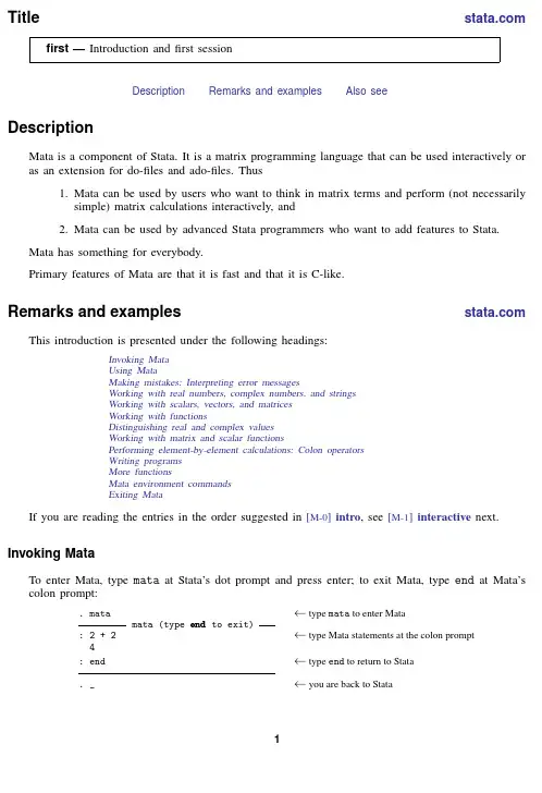
Title first—Introduction andfirst sessionDescription Remarks and examples Also seeDescriptionMata is a component of Stata.It is a matrix programming language that can be used interactively or as an extension for do-files and ado-files.Thus1.Mata can be used by users who want to think in matrix terms and perform(not necessarilysimple)matrix calculations interactively,and2.Mata can be used by advanced Stata programmers who want to add features to Stata.Mata has something for everybody.Primary features of Mata are that it is fast and that it is C-like.Remarks and examples This introduction is presented under the following headings:Invoking MataUsing MataMaking mistakes:Interpreting error messagesWorking with real numbers,complex numbers,and stringsWorking with scalars,vectors,and matricesWorking with functionsDistinguishing real and complex valuesWorking with matrix and scalar functionsPerforming element-by-element calculations:Colon operatorsWriting programsMore functionsMata environment commandsExiting MataIf you are reading the entries in the order suggested in[M-0]intro,see[M-1]interactive next. Invoking MataTo enter Mata,type mata at Stata’s dot prompt and press enter;to exit Mata,type end at Mata’s colon prompt:.mata←type mata to enter Matamata(type end to exit):2+2←type Mata statements at the colon prompt4:end←type end to return to Stata._←you are back to Stata12first—Introduction andfirst sessionUsing MataWhen you type a statement into Mata,Mata compiles what you typed and,if it compiled without error,executes it::2+24:_We typed2+2,a particular example from the general class of expressions.Mata responded with4, the evaluation of the expression.Often what you type are expressions,although you will probably choose more complicated examples.When an expression is not assigned to a variable,the result of the expression is displayed.Assignment is performed by the=operator::x=2+2:x4:_When we type“x=2+2”,the expression is evaluated and stored in the variable we just named x.The result is not displayed.We can look at the contents of x,however,simply by typing“x”.From Mata’s perspective,x is not only a variable but also an expression,albeit a rather simple one.Just as 2+2says to load2,load another2,and add them,the expression x says to load x and stop there.As an aside,Mata distinguishes uppercase and lowercase.X is not the same as x::X=2+3:x4:X5:_Making mistakes:Interpreting error messagesIf you make a mistake,Mata complains,and then you continue on your way.For instance, :2,,3invalid expressionr(3000);:_2,,3makes no sense to Mata,so Mata complained.This is an example of what is called a compile-time error;Mata could not make sense out of what we typed.The other kind of error is called a run-time error.For example,we have no variable called y.Let us ask Mata to show us the contents of y::y<istmt>:3499y not foundr(3499);:_first—Introduction andfirst session3 Here what we typed made perfect sense—show me y—but y has never been defined.This ugly message is called a run-time error message—see[M-2]errors for a complete description—but all that’s important is to understand the difference betweeninvalid expressionand<istmt>:3499y not foundThe run-time message is prefixed by an identity(<istmt>here)and a number(3499here).Mata is telling us,“I was executing your istmt[that’s what everything you type is called]and I got error 3499,the details of which are that I was unable tofind y.”The compile-time error message is of a simpler form:invalid expression.When you get such unprefixed error messages,that means Mata could not understand what you typed.When you get the more complicated error message,that means Mata understood what you typed,but there was a problem performing your request.Another way to tell the difference between compile-time errors and run-time errors is to look at the return pile-time errors have a return code of3000::2,,3invalid expressionr(3000);Run-time errors have a return code that might be in the3000s,but is never3000exactly: :y<istmt>:3499y not foundr(3499);Whether the error is compile-time or run-time,once the error message is issued,Mata is ready to continue just as if the error never happened.Working with real numbers,complex numbers,and stringsAs we have seen,Mata works with real numbers::2+35Mata also understands complex numbers;you write the imaginary part by suffixing a lowercase i: :1+2i+4-1i5+1iFor imaginary numbers,you can omit the real part::1+2i-2i1Whether a number is real or complex,you can use the same computer notation for the imaginary part as you would for the real part::2.5e+3i2500i:1.25e+2+2.5e+3i/*i.e.,1.25+e02+2.5e+03i*/125+2500i4first—Introduction andfirst sessionWe purposely wrote the last example in nearly unreadable form just to emphasize that Mata could interpret it.Mata also understands strings,which you write enclosed in double quotes::"Alpha"+"Beta"AlphaBetaJust like Stata,Mata understands simple and compound double quotes::‘"Alpha"’+‘"Beta"’AlphaBetaYou can add complex and reals,:1+2i+34+2ibut you may not add reals or complex to strings::2+"alpha"type mismatch:real+string not allowedr(3000);We got a run-time error.Mata understood2+"alpha"all right;it just could not perform our request. Working with scalars,vectors,and matricesIn addition to understanding scalars—be they real,complex,or string—Mata understands vectors and matrices of real,complex,and string elements::x=(1,2):x12112x now contains the row vector(1,2).We can add vectors::x+(3,4)12146The“,”is the column-join operator;things like(1,2)are expressions,just as(1+2)is an expression::y=(3,4):z=(x,y):z123411234In the above,we could have dispensed with the parentheses and typed“y=3,4”followed by“z= x,y”,just as we could using the+operator,although most peoplefind vectors more readable when enclosed in parentheses.first—Introduction andfirst session5\is the row-join operator::a=(1\2):a11122::b=(3\4):c=(a\b):c111223344Using the column-join and row-join operators,we can enter matrices::A=(1,2\3,4):A12112234The use of these operators is not limited to scalars.Remember,x is the row vector(1,2),y is the row vector(3,4),a is the column vector(1\2),and b is the column vector(3\4).Therefore, :x\y12112234:a,b12113224But if we try something nonsensical,we get an error::a,x<istmt>:3200conformability errorWe create complex vectors and matrices just as we create real ones,the only difference being that their elements are complex::Z=(1+1i,2+3i\3-2i,-1-1i):Z1211+1i2+3i23-2i-1-1i6first—Introduction andfirst sessionSimilarly,we can create string vectors and matrices,which are vectors and matrices with string elements::S=("1st element","2nd element"\"another row","last element"):S1211st element2nd element2another row last elementFor strings,the individual elements can be up to2,147,483,647characters long.Working with functionsMata’s expressions also include functions::sqrt(4)2:sqrt(-4).When we ask for the square root of−4,Mata replies“.”Further,.can be stored just like any other number::findout=sqrt(-4):findout.“.”means missing,that there is no answer to our calculation.Taking the square root of a negative number is not an error;it merely produces missing.To Mata,missing is a number like any other number,and the rules for all the operators have been generalized to understand missing.For instance, the addition rule is generalized such that missing plus anything is missing::2+..Still,it should surprise you that Mata produced missing for the sqrt(-4).We said that Mata understands complex numbers,so should not the answer be2i?The answer is that is should be if you are working on the complex plane,but otherwise,missing is probably a better answer.Mata attempts to intuit the kind of answer you want by context,and in particular,uses inheritance rules.If you ask for the square root of a real number,you get a real number back.If you ask for the square root of a complex number,you get a complex number back::sqrt(-4+0i)2iHere complex means multipart:-4+0i is a complex number;it merely happens to have0imaginary part.Thus::areal=-4:acomplex=-4+0i:sqrt(areal).:sqrt(acomplex)2ifirst—Introduction andfirst session7 If you ever have a real scalar,vector,or matrix,and want to make it complex,use the C()function, which means“convert to complex”::sqrt(C(areal))2iC()is documented in[M-5]C().C()allows one or two arguments.With one argument,it casts to complex.With two arguments,it makes a complex out of the two real arguments.Thus you could type:sqrt(-4+2i).485868272+2.05817103ior you could type:sqrt(C(-4,2)).485868272+2.05817103iBy the way,used with one argument,C()also allows complex,and then it does nothing: :sqrt(C(acomplex))2iDistinguishing real and complex valuesIt is virtually impossible to tell the difference between a real value and a complex value with zero imaginary part::areal=-4:acomplex=-4+0i:areal-4:acomplex-4Yet,as we have seen,the difference is important:sqrt(areal)is missing,sqrt(acomplex)is 2i.One solution is the eltype()function::eltype(areal)real:eltype(acomplex)complexeltype()can also be used with strings,:astring="hello":eltype(astring)stringbut this is useful mostly in programming contexts.8first—Introduction andfirst sessionWorking with matrix and scalar functionsSome functions are matrix functions:they require a matrix and return a matrix.Mata’s invsym(X) is an example of such a function.It returns the matrix that is the inverse of symmetric,real matrix X: :X=(76,53,48\53,88,46\48,46,63):Xi=invsym(X):Xi[symmetric]1231.029*******2-.0098470272.021*******3-.0155497706-.0082885675.0337724301:Xi*X12311-8.67362e-17-8.50015e-172-1.38778e-161-1.02349e-1630 1.11022e-161The last matrix,Xi*X,differs just a little from the identity matrix because of unavoidable computational roundoff error.Other functions are,mathematically speaking,scalar functions.sqrt()is an example in that it makes no sense to speak of sqrt(X).(That is,it makes no sense to speak of sqrt(X)unless we were speaking of the Cholesky square-root decomposition.Mata has such a matrix function;see [M-5]cholesky().)When a function is,mathematically speaking,a scalar function,the corresponding Mata function will usually allow vector and matrix arguments and,then,the Mata function makes the calculation on each element individually::M=(1,2\3,4\5,6):M12112234356::S=sqrt(M):S1211 1.4142135622 1.73205080823 2.236067977 2.449489743::S[1,2]*S[1,2]2:S[2,1]*S[2,1]3first—Introduction andfirst session9 When a function returns a result calculated in this way,it is said to return an element-by-element result.Performing element-by-element calculations:Colon operatorsMata’s operators,such as+(addition)and*(multiplication),work as you would expect.In particular, *performs matrix multiplication::A=(1,2\3,4):B=(5,6\7,8):A*B121192224350Thefirst element of the result was calculated as1∗5+2∗7=19.Sometimes,you really want the element-by-element result.When you do,place a colon in front of the operator:Mata’s:*operator performs element-by-element multiplication::A:*B12151222132See[M-2]op colon for more information.Writing programsMata is a complete programming language;it will allow you to create your own functions: :function add(a,b)return(a+b)That single statement creates a new function,although perhaps you would prefer if we typed it as :function add(a,b)>{>return(a+b)>}because that makes it obvious that a program can contain many lines.In either case,once defined, we can use the function::add(1,2)3:add(1+2i,4-1i)5+1i:add((1,2),(3,4))1214610first—Introduction andfirst session:add(x,y)12146:add(A,A)12124268::Z1=(1+1i,1+1i\2,2i):Z2=(1+2i,-3+3i\6i,-2+2i):add(Z1,Z2)1212+3i-2+4i22+6i-2+4i::add("Alpha","Beta")AlphaBeta::S1=("one","two"\"three","four"):S2=("abc","def"\"ghi","jkl"):add(S1,S2)121oneabc twodef2threeghi fourjklOf course,our little function add()does not do anything that the+operator does not already do, but we could write a program that did do something different.The following program will allow us to make n×n identity matrices::real matrix id(real scalar n)>{>real scalar i>real matrix res>>res=J(n,n,0)>for(i=1;i<=n;i++){>res[i,i]=1>}>return(res)>}::I3=id(3):I3[symmetric]123112013001The function J()in the program line res=J(n,n,0)is a Mata built-in function that returns an n×n matrix containing0s(J(r,c,val)returns an r×c matrix,the elements of which are all equal to val);see[M-5]J().for(i=1;i<=n;i++)says that starting with i=1and so long as i<=n do what is inside the braces(set res[i,i]equal to1)and then(we are back to the for part again),increment i.Thefinal line—return(res)—says to return the matrix we have just created.Actually,just as with add(),we do not need id()because Mata has a built-in function I(n)that makes identity matrices,but it is interesting to see how the problem could be programmed.More functionsMata has many functions already and much of this manual concerns documenting what those functions do;see[M-4]intro.But right now,what is important is that many of the functions are themselves written in Mata!One of those functions is pi();it takes no arguments and returns the value of pi.The code for it readsreal scalar pi()return(3.141592653589793238462643)There is no reason to type the above function because it is already included as part of Mata: :pi()3.141592654When Mata lists a result,it does not show as many digits,but we could ask to see more: :printf("%17.0g",pi())3.14159265358979Other Mata functions include the hyperbolic function tanh(u).The code for tanh(u)reads numeric matrix tanh(numeric matrix u){numeric matrix eu,emueu=exp(u)emu=exp(-u)return((eu-emu):/(eu+emu))}See for yourself:at the Stata dot prompt(not the Mata colon prompt),type.viewsource tanh.mataWhen the code for a function was written in Mata(as opposed to having been written in C), viewsource can show you the code;see[M-1]source.Returning to the function tanh(),numeric matrix tanh(numeric matrix u){numeric matrix eu,emueu=exp(u)emu=exp(-u)return((eu-emu):/(eu+emu))}this is thefirst time we have seen the word numeric:it means real or complex.Built-in(previously written)function exp()works like sqrt()in that it allows a real or complex argument and correspondingly returns a real or complex result.Said in Mata jargon:exp()allows a numeric argument and correspondingly returns a numeric result.tanh()will also work like sqrt()and exp().Another characteristic tanh()shares with sqrt()and exp()is element-by-element operation. tanh()is element-by-element because exp()is element-by-element and because we were careful to use the:/(element-by-element)divide operator.In any case,there is no need to type the above functions because they are already part of Mata.You could learn more about them by seeing their manual entry,[M-5]sin().At the other extreme,Mata functions can become long.Here is Mata’s function to solve AX=B for X when A is lower triangular,placing the result X back into A:real scalar_solvelower(numeric matrix A,numeric matrix b,|real scalar usertol,numeric scalar userd){real scalar tol,rank,a_t,b_t,d_treal scalar n,m,i,im1,complex_casenumeric rowvector sumnumeric scalar zero,dd=userdif((n=rows(A))!=cols(A))_error(3205)if(n!=rows(b))_error(3200)if(isview(b))_error(3104)m=cols(b)rank=na_t=iscomplex(A)b_t=iscomplex(b)d_t=d<.?iscomplex(d):0complex_case=a_t|b_t|d_tif(complex_case){if(!a_t)A=C(A)if(!b_t)b=C(b)if(d<.&!d_t)d=C(d)zero=0i}else zero=0if(n==0|m==0)return(0)tol=solve_tol(A,usertol)if(abs(d)>=.){if(abs(d=A[1,1])<=tol){b[1,.]=J(1,m,zero)--rank}else{b[1,.]=b[1,.]:/dif(missing(d))rank=.}for(i=2;i<=n;i++){im1=i-1sum=A[|i,1ı,im1|]*b[|1,1\im1,m|]if(abs(d=A[i,i])<=tol){b[i,.]=J(1,m,zero)--rank}else{b[i,.]=(b[i,.]-sum):/dif(missing(d))rank=.}}}else{if(abs(d)<=tol){rank=0b=J(rows(b),cols(b),zero)}else{b[1,.]=b[1,.]:/dfor(i=2;i<=n;i++){im1=i-1sum=A[|i,1ı,im1|]*b[|1,1\im1,m|]b[i,.]=(b[i,.]-sum):/d}}}return(rank)}If the function were not already part of Mata and you wanted to use it,you could type it into a do-file or onto the end of an ado-file(especially good if you just want to use solvelower()as a subroutine).In those cases,do not forget to enter and exit Mata:begin ado-fileprogram mycommand...ado-file code appears here...endmata:_solvelower()code appears hereendend ado-file Sharp-eyed readers will notice that we put a colon on the end of the Mata command.That’s a detail, and why we did that is explained in[M-3]mata.In addition to loading functions by putting their code in do-and ado-files,you can also save the compiled versions of functions in.mofiles(see[M-3]mata mosave)or into.mlib Mata libraries (see[M-3]mata mlib).For solvelower(),it has already been saved into a library,namely,Mata’s official library,so you need not do any of this.Mata environment commandsWhen you are using Mata,there is a set of commands that will tell you about and manipulate Mata’s environment.The most useful such command is mata describe;see[M-3]mata describe::mata describe#bytes type name and extent76transmorphic matrix add()200real matrix id()32real matrix A[2,2]32real matrix B[2,2]72real matrix I3[3,3]48real matrix M[3,2]48real matrix S[3,2]47string matrix S1[2,2]44string matrix S2[2,2]72real matrix X[3,3]72real matrix Xi[3,3]64complex matrix Z[2,2]64complex matrix Z1[2,2]64complex matrix Z2[2,2]16real colvector a[2]16complex scalar acomplex8real scalar areal16real colvector b[2]32real colvector c[4]8real scalar findout16real rowvector x[2]16real rowvector y[2]32real rowvector z[4]:_Another useful command is mata clear(see[M-3]mata clear),which will clear Mata without disturbing Stata::mata clear:mata describe#bytes type name and extentThere are other useful mata commands;see[M-3]intro.Do not confuse this command mata,which you type at Mata’s colon prompt,with Stata’s command mata,which you type at Stata’s dot prompt and which invokes Mata.Exiting MataWhen you are done using Mata,type end to Mata’s colon prompt::end._Exiting Mata does not clear it:.matamata(type end to exit):x=2:y=(3+2i):function add(a,b)return(a+b):end.....matamata(type end to exit):mata describe#bytes type name and extent76transmorphic matrix add()8real scalar x16complex scalar y:endExiting Stata clears Mata,as does Stata’s clear mata command;see[D]clear.Also see[M-1]intro—Introduction and advice。

领先一期变量?gendydy?gendyy?ly或者y?yn?112作图?twowayscatteryp?twowaylineyp?histogramybin2013回归?regressypith?regressypithifyear1970?regressypithnoconstant?regressypithbeta14其他的回归命令?areganeasierwaytofitregressionswithmanydummyvariables?archregressionmodelswitharcherrors?arimaarimamodels?boxcoxbox?coxregressionmodels?cnregcensored?normalregression?cnsregconstrainedlinearregression?eivregerrors?in?variablesregression?frontierstochasticfrontiermodels?heckmanheckmanselectionmodel?intregintervalregression?ivregresssingle?equationinstrumental?variablesregression?ivtobittobitregressionwithendogenousvariables?neweyregressionwithnewey?weststandarderrors?qregquantileincludingmedianregression?reg3three?stageleast?squares3slsregression?rregatypeofrobustregression?suregseeminglyunrelatedregression?tobittobitregression?treatregtreatment?effectsmodel?truncregtruncatedregression?xtabondarellano?bondlineardynamicpanel?dataestimation?xtdpdlineardynamicpanel?dataestimation?xtfrontierpanel?datastochasticfrontiermodel?xtglspanel?dataglsmode

• summarize mpg • return list • scalar avgmpg=r(mean)
• Regression:
• • • •
regress mpg weight ereturn list scalar obs=e(N) scalar beta1=_b[weight]
Introduction to Stata
• Declare a variable
• scalar example=3 • display 2+example
• View a subset of the sample
• list in 1/10 • list if mpg<14
• Frequency of observations
• tabulate mpg
• Use menu, then copy to .do file
Introduction to Stata
P RACTICE P ROBLEM
• Wooldridge C2.2 • summarize salary ceoten • tabulate ceoten • regress salary ceoten • generate salary2 = salary*1000 • drop lsalary • generate lsalary = log(salary)
• rename var1 log_dollars • label variable log_dollars “Natural log of dollars spent o • generate dollars = exp(dollars) • Run regressions
Introduction to Stata

2
In STATA you can refer to each variable by the variable name. You can also refer to the line number by using the reference “in”. Exercise; Write the commands list make in 2, list weight in 1/7. What is returned in the results window?
The help faciliபைடு நூலகம்y
• • • You can use Viewer to open a help file and enter commands in the Command window Use Help - Contents or Stata Command from the main Menu bar and enter commands in the Command window (you get information on how to use the command) Use Help from the main Menu bar and choose Search from the Help menu (you get references-links to all related Stata commands in the Reference Manual, User’s guide and Programming manual). Use proper statistical terminology.
ECON 4135, 2009
A quick introduction to STATA

Stata入门介绍Stata入门介绍转载，原作者不详。

(1) Stata要在使用中熟练的，大家应该多加练习。

(2) Stata的很多细节，这里不会涉及，只是选取相对重要的部分加以解释，大家在使用Stata过程中留心积累。

作为入门性质的介绍，本文只选取和中级计量经济学作业相关的内容和一些处理数据所使用的基本命令。

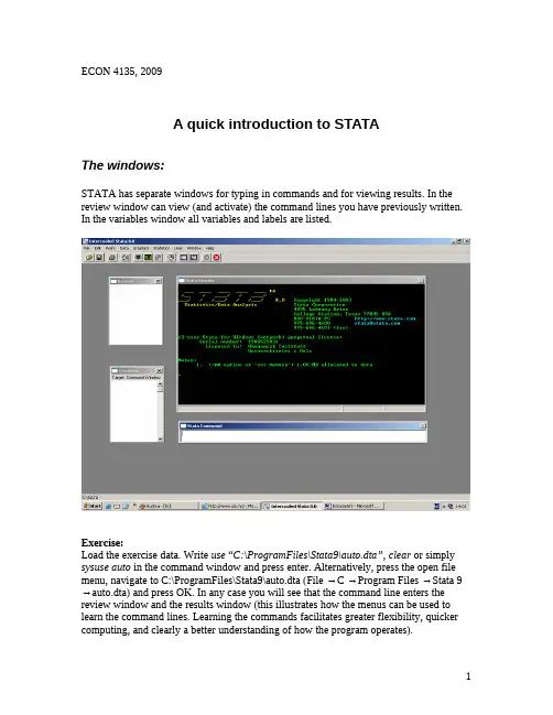
对于更高深的内容，请大家参看STATA manual.”界面当我们把stata装好以后，首先需要了解的是它的界面。

打开Stata后我们便可以看到它常用的四个窗口：Stata Results; Review; Variables; Stata Command。

我们所有的运行结果都会在Stata Results界面中显示；而命令的输入则在Stata Command窗口；Review窗口记录我们使用过的命令；最后Variables窗口显示存在于当前数据库中的所有变量的名称。

可以直接点击 Review窗口来重新输入已使用过的命令，我们所需变量可以通过点击Varaibles窗口来得到，这些都可以简便我们的操作。

Stata 命令Stata软件功能强大，体现在它提供了丰富的命令，可以实现许多功能。

每一个stata命令都相应的命令格式。

我们在这里介绍常用的一些命令的功能和相应的格式，大家在使用stata的过程中会不断积累命令的相关知识。

需要对命令的帮助时可以用help命令查询。

例如了解命令：“reg” ，就可以在Stata Command窗口输入“help reg” ，也可以在Help选项下content中查找我们需要的相关命令。

用help查询，则窗口会显示关于该命令的详尽说明。

更直接的办法是看Examples中的范例是如何使用该命令，阅读一些相关的说明并加以模仿。

重要习惯我们使用stata进行回归分析时，需要养成一些好的习惯。

在进行一些数据量很大，过程复杂的分析时尤其重要。

（1）使用日志（log）。

它可以帮助我们记录stata的运行结果。

18Learning more about StataWhere to go from hereYou now know plenty enough to use Stata.There is still much,much more to learn because Stata is a rich environment for doing statistical analysis and data management.What should you do to learn more?•Get an interesting dataset and play with Stata.e the menus and dialog system to experiment with commands.Notice what commandsshow up in the Results window.You willfind that Stata’s simple and consistent commandsyntax will make the commands easy to read so that you will know what you have doneand easy to remember so that typing some commands will be faster than using menus.b.Play with graphs and the Graph Editor.•If you venture into the Command window,you willfind that many things will go faster.You will alsofind that it is possible to make mistakes where you cannot understand why Stata is balking.a.Try help commandname or Help>Stata command...and entering the command name.b.Look at the command syntax and the examples in the helpfile,and compare themwith what you pare them closely:small typographical errors make commandsimpossible for Stata to parse.•Explore Stata by selecting Help>Search....You will uncover many statistical routines that could be of great use.•Look through the Combined subject table of contents in the Stata Index.•Read and work your way through the User’s Guide.It is designed to be read from cover to cover,and it contains most of the information you need to become an expert Stata user.It is well worth reading.If you are not this ambitious and instead prefer to sample the User’s Guide and the references,there is some advice later in this chapter for you.•Browse through the reference manuals to read about statistical methods you like to use,making use of the links to jump to other topics.The reference manuals are not meant to be read from cover to cover—they are meant to be referred to as you would an encyclopedia.You canfind the datasets used in the examples in the manuals by selecting File>Example datasets...and then clicking on Stata18manual datasets.Doing so will enable you to work through the examples quickly.•Stata has much information,including answers to frequently asked questions(FAQ s),at https:///support/faqs/.•There are many useful links to Stata resources at https:///links/.Be sure to look at these materials because many outstanding resources about Stata are listed here.•Join Statalist,a forum devoted to discussion of Stata and statistics.•Read The Stata Blog:Not Elsewhere Classified at https:// to read articles written by people at Stata about all things Stata.•Visit Stata on Facebook at https:///statacorp,join Stata on Instagram at https:///statacorp,find Stata on LinkedIn at https:///company/statacorp,and follow Stata on Twitter at https:///stata to keep up with Stata.•Subscribe to the Stata Journal,which contains reviewed papers,regular columns,book reviews, and other material of interest to researchers applying statistics in a variety of disciplines.Visit https://.12[GSM]18Learning more about Stata•Many supplementary books about Stata are available.Visit the Stata Bookstore athttps:///bookstore/.•Take a Stata NetCourse R .NetCourse101is an excellent choice for learning about Stata.See https:///netcourse/for course information and schedules.•Attend a classroom or a web-based training course taught by StataCorp.Visithttps:///training/classroom-and-web/for course information and schedules.•View a webinar led by Stata developers.Visit https:///training/webinar/for the current list of topics and schedule.•Watch Stata videos at https:///user/statacorp.Suggested reading from the User’s Guide and reference manuals The User’s Guide is designed to be read from cover to cover.The reference manuals are designed as references to be sampled when necessary.Ideally,after reading this Getting Started manual,you should read the User’s Guide from cover to cover,but you probably want to become at least somewhat proficient in Stata right away.Here isa suggested reading list of sections from the User’s Guide and the reference manuals to help you onyour way to becoming a Stata expert.This list covers fundamental features and points you to some less obvious features that you might otherwise overlook.Basic elements of Stata[U]11Language syntax[U]12Data[U]13Functions and expressionsData management[U]6Managing memory[U]22Entering and importing data[D]import—Overview of importing data into Stata[D]append—Append datasets[D]merge—Merge datasets[D]compress—Compress data in memory[D]frames intro—Introduction to framesGraphics[G]Stata Graphics Reference ManualReproducible research[U]16Do-files[U]17Ado-files[U]13.5Accessing coefficients and standard errors[U]13.6Accessing results from Stata commands[U]21Creating reports[RPT]Dynamic documents intro—Introduction to dynamic documents[RPT]putdocx intro—Introduction to generating Office Open XML(.docx)files[RPT]putexcel—Export results to an Excelfile[RPT]putpdf intro—Introduction to generating PDFfiles[R]log—Echo copy of session tofile[GSM]18Learning more about Stata3Useful features that you might overlook[U]29Using the Internet to keep up to date[U]19Immediate commands[U]24Working with strings[U]25Working with dates and times[U]26Working with categorical data and factor variables[U]27Overview of Stata estimation commands[U]20Estimation and postestimation commands[R]estimates—Save and manipulate estimation resultsBasic statistics[R]anova—Analysis of variance and covariance[R]ci—Confidence intervals for means,proportions,and variances[R]correlate—Correlations of variables[D]egen—Extensions to generate[R]regress—Linear regression[R]predict—Obtain predictions,residuals,etc.,after estimation[R]regress postestimation—Postestimation tools for regress[R]test—Test linear hypotheses after estimation[R]summarize—Summary statistics[R]table intro—Introduction to tables of frequencies,summaries,and command results [R]tabulate oneway—One-way table of frequencies[R]tabulate twoway—Two-way table of frequencies[R]ttest—t tests(mean-comparison tests)Matrices[U]14Matrix expressions[U]18.5Scalars and matrices[M]Mata Reference ManualProgramming[U]16Do-files[U]17Ado-files[U]18Programming Stata[R]ml—Maximum likelihood estimation[P]Stata Programming Reference Manual[M]Mata Reference ManualSystem values[R]set—Overview of system parameters[P]creturn—Return c-class values4[GSM]18Learning more about StataInternet resourcesThe Stata website(https://)is a good place to get more information about Stata.You willfind answers to FAQ s,ways to interact with other users,official Stata updates,and other useful information.You can also join Statalist,a forum devoted to discussion of Stata and statistics.You will alsofind information on Stata NetCourses R ,which are interactive courses offered over the Internet that vary in length from a few weeks to eight weeks.Stata also offers in-person and web-based training sessions,as well as webinars on Stata features.Visit https:///learn/ for more information.At the website is the Stata Bookstore,which contains books that we feel may be of interest to Stata users.Each book has a brief description written by a member of our technical staff explaining why we think this book may be of interest.We suggest that you take a quick look at the Stata website now.You can register your copy of Stata online and request a free subscription to the Stata News.Visit https:// for information on books,manuals,and journals published by Stata Press.The datasets used in examples in the Stata manuals are available from the Stata Press website.Also visit https:// to read about the Stata Journal,a quarterly publication containing articles about statistics,data analysis,teaching methods,and effective use of Stata’s language.Visit Stata’s official blog at https:// for news and advice related to the use of Stata.The articles appearing in the blog are individually signed and are written by the same people who develop,support,and sell Stata.The Stata Blog:Not Elsewhere Classified also has links to other blogs about Stata,written by Stata users around the world.Follow Stata on Facebook at https:///statacorp,Twitter at https:///stata, Instagram at https:///statacorp,and LinkedIn athttps:///company/statacorp.You may also follow Stata on Twitter athttps:///stata fr or https:///stata es.These are good ways to stay up-to-the-minute with the latest Stata information.Watch short example videos of using Stata on YouTube at https:///user/statacorp.See[GSM]19Updating and extending Stata—Internet functionality for details on accessing official Stata updates and free additions to Stata on the Stata website.[GSM]18Learning more about Stata5 Stata,Stata Press,and Mata are registered trademarks of StataCorp LLC.Stata andStata Press are registered trademarks with the World Intellectual Property Organization®of the United Nations.Other brand and product names are registered trademarks ortrademarks of their respective companies.Copyright c 1985–2023StataCorp LLC,College Station,TX,USA.All rights reserved.。

-----------------------------------------------------------------------------------------------------------------

1. STATA: INTRODUCTION This tutorial will introduce you to a statistical and econometric software package called STATA. The tutorial is an introduction to some of the most commonly used features in STATA. These features were used by the authors of your textbook to generate the statistical analysis report in Chapters 3-9 (Stock and Watson, 2011). The tutorial provides the necessary background to reproduce the results of Chapters 3-9 and to carry out related exercises. It does not cover panel data (Chapter 10), binary dependent variables (Chapter 11), instrumental variable analysis (Chapter 12), or time-series analysis (Chapters 14-16). The most current professional version is STATA 11. Both STATA 10 and 11 are sufficiently similar so that those who have access to STATA 11 can use this tutorial for the more advanced version. As with many statistical packages, newer versions allow you to use more advanced and recently developed techniques that you, as a first time user, most likely will not encounter in a first course of econometrics. There are several versions of STATA 10 and 11, such as STATA/IC, STATA/SE, and STATA/MP. The difference is basically in terms of the number of variables STATA can handle and the speed at which information is processed. Most users will probably work with the “Intercooled” (IC) version. STATA runs on the Windows (2000, 2003, XP, Vista, Server 2008, or Windows 7), Mac, and Unix computers platform. I assume most of you will be using STATA on Windows computers. It is produced by StataCorp in College Station, TX. You can read about various product information at the firm’s Web site, . There are 19 manuals that can be purchased with STATA 11, although subsets can be bought separately. Perhaps the most useful of these are the User’s Guide and three volumes of the Base Reference Manuals ($210 together). You can order STATA by calling (800) 782-8272 or writing to service@. In addition, if you purchase the Student Version (“GradPlans”), you can acquire STATA at a steep discount. Prices vary, but you could get a “perpetual license” for STATA/IC for $179, or a six-month license for as low as $65. Econometrics deals with three types of data: cross-sectional data, time series data, and panel (longitudinal) data (see Chapter 1 of the Stock and Watson (2011)). In a cross-section you analyze data from multiple entities at a single point in time. In a time series you observe the behavior of a single entity over multiple time periods. This can range from high frequency data such as financial data (hours, days); to data observed at somewhat lower (monthly) frequencies, such as industrial production, inflation, and unemployment rates; to quarterly data (GDP) or annual (historical) data. One big difference between cross-sectional and time series analysis is that the order of the observation numbers does not matter in cross-sections. With time series, you would lose some of the most interesting features of the data if you shuffled the observations. Finally, panel data can be viewed as a combination of cross-sectional and time series data, since multiple entities are observed at multiple time periods. STATA allows you to work with all three types of data. STATA is most commonly used for cross-sectional and panel data in academics, business, and government, but you can work with it relatively easily when you analyze time-series data.

Stata操作讲义第一讲Stata操作入门第一节概况Stata最初由美国计算机资源中心（Computer Resource Center）研制，现在为Stata公司的产品，其最新版本为7.0版。

它操作灵活、简单、易学易用，是一个非常有特色的统计分析软件，现在已越来越受到人们的重视和欢迎，并且和SAS、SPSS一起，被称为新的三大权威统计软件。

Stata最为突出的特点是短小精悍、功能强大，其最新的7.0版整个系统只有10M左右，但已经包含了全部的统计分析、数据管理和绘图等功能，尤其是他的统计分析功能极为全面，比起1G以上大小的SAS系统也毫不逊色。

另外，由于Stata在分析时是将数据全部读入内存，在计算全部完成后才和磁盘交换数据，因此运算速度极快。

由于Stata的用户群始终定位于专业统计分析人员，因此他的操作方式也别具一格，在Windows席卷天下的时代，他一直坚持使用命令行／程序操作方式，拒不推出菜单操作系统。

但是，Stata的命令语句极为简洁明快，而且在统计分析命令的设置上又非常有条理，它将相同类型的统计模型均归在同一个命令族下，而不同命令族又可以使用相同功能的选项，这使得用户学习时极易上手。

更为令人叹服的是，Stata语句在简洁的同时又拥有着极高的灵活性，用户可以充分发挥自己的聪明才智，熟练应用各种技巧，真正做到随心所欲。

除了操作方式简洁外，Stata的用户接口在其他方面也做得非常简洁，数据格式简单，分析结果输出简洁明快，易于阅读，这一切都使得Stata成为非常适合于进行统计教学的统计软件。

Stata的另一个特点是他的许多高级统计模块均是编程人员用其宏语言写成的程序文件（ADO文件），这些文件可以自行修改、添加和下载。

用户可随时到Stata网站寻找并下载最新的升级文件。

事实上，Stata的这一特点使得他始终处于统计分析方法发展的最前沿，用户几乎总是能很快找到最新统计算法的Stata程序版本，而这也使得Stata自身成了几大统计软件中升级最多、最频繁的一个。

stata 10%分位数摘要：一、引言1.了解Stata 10%分位数的重要性2.文章目的：提供Stata 10%分位数的详细操作方法二、Stata 10%分位数计算方法1.定义：将数据集按照数值大小排序2.计算：从大到小依次选取10%的样本三、操作步骤1.打开Stata软件2.输入命令：`infile`3.导入数据：`use`4.排序：`sort`5.计算10%分位数：`quantile`6.输出结果：`list`四、实例演示1.下载示例数据2.按照步骤操作，查看结果五、结果解释1.10%分位数含义：低于这个数值的样本占全体的10%2.分析结果：与均值、中位数等指标结合，全面了解数据分布六、注意事项1.数据预处理：确保数据质量，剔除异常值2.区分10%、25%、50%等分位数：各有用途，根据需求选择七、总结1.掌握Stata 10%分位数计算方法2.提高数据分析能力，为实证研究提供有力支持正文：作为一名职业写手，今天我们将为大家介绍如何在Stata软件中计算10%分位数。

分位数是一种描述数据分布状况的统计量，可以帮助我们更好地了解数据的整体情况。

在实际应用中，10%分位数常常被用来衡量数据的极端情况，以便我们更好地制定决策。

以下是计算Stata 10%分位数的详细步骤：1.打开Stata软件，进入操作界面。

2.输入命令`infile`，表示要导入文件。

接着输入文件路径，例如：`infile "D:data.dta"`。

3.导入数据。

输入命令`use`，软件会自动读取数据并显示在界面上。

4.对数据进行排序。

输入命令`sort`，数据会按照数值大小进行升序排列。

5.计算10%分位数。

输入命令`quantile`，然后按Enter键。

此时，Stata 会自动计算出10%分位数，并将其保存在变量`p10`中。

6.输出结果。

输入命令`list`，然后按Enter键。

此时，我们可以看到包含10%分位数的结果出现在界面上。

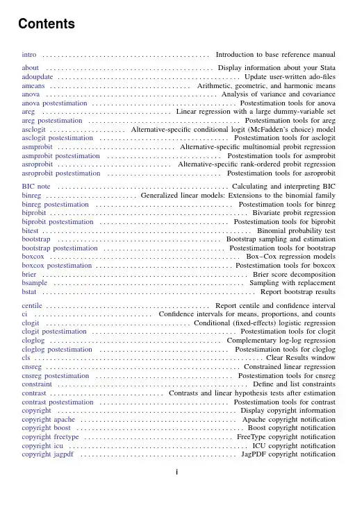
Contentsintro............................................Introduction to base reference manual about............................................Display information about your Stata adoupdate................................................Update user-written ado-files ameans.....................................Arithmetic,geometric,and harmonic means anova.............................................Analysis of variance and covariance anova postestimation......................................Postestimation tools for anova areg..................................Linear regression with a large dummy-variable set areg postestimation........................................Postestimation tools for areg asclogit....................Alternative-specific conditional logit(McFadden’s choice)model asclogit postestimation..................................Postestimation tools for asclogit asmprobit...............................Alternative-specific multinomial probit regression asmprobit postestimation..............................Postestimation tools for asmprobit asroprobit..............................Alternative-specific rank-ordered probit regression asroprobit postestimation..............................Postestimation tools for asroprobit BIC note.............................................Calculating and interpreting BIC binreg........................Generalized linear models:Extensions to the binomial family binreg postestimation....................................Postestimation tools for binreg biprobit....................................................Bivariate probit regression biprobit postestimation..................................Postestimation tools for biprobit bitest.......................................................Binomial probability test bootstrap...........................................Bootstrap sampling and estimation bootstrap postestimation................................Postestimation tools for bootstrap boxcox..................................................Box–Cox regression models boxcox postestimation....................................Postestimation tools for boxcox brier......................................................Brier score decomposition bsample..................................................Sampling with replacement bstat........................................................Report bootstrap results centile...........................................Report centile and confidence interval ci...............................Confidence intervals for means,proportions,and counts clogit......................................Conditional(fixed-effects)logistic regression clogit postestimation......................................Postestimation tools for clogit plementary log-log regression cloglog postestimation..................................Postestimation tools for cloglog cls............................................................Clear Results window cnsreg...................................................Constrained linear regression cnsreg postestimation....................................Postestimation tools for cnsreg constraint..................................................Define and list constraints contrast..............................Contrasts and linear hypothesis tests after estimation contrast postestimation..................................Postestimation tools for contrast copyright...............................................Display copyright information copyright apache.........................................Apache copyright notification copyright boost............................................Boost copyright notification copyright freetype.......................................FreeType copyright notification copyright icu...............................................ICU copyright notification copyright jagpdf.........................................JagPDF copyright notificationiii Contentscopyright PACK copyright notification copyright libpng..........................................libpng copyright notification copyright miglayout..................................MiG Layout copyright notification copyright scintilla........................................Scintilla copyright notification copyright ttf2pt1..........................................ttf2pt1copyright notification copyright zlib..............................................zlib copyright notification correlate.............................Correlations(covariances)of variables or coefficients cumul.......................................................Cumulative distribution cusum........................................Cusum plots and tests for binary variables unch dialog diagnostic plots..........................................Distributional diagnostic plots display................................................Substitute for a hand calculator do....................................................Execute commands from afile doedit................................................Edit do-files and other textfiles parative scatterplots dstdize.............................................Direct and indirect standardization dydx........................................Calculate numeric derivatives and integrals eform option......................................Displaying exponentiated coefficients eivreg...................................................Errors-in-variables regression eivreg postestimation.....................................Postestimation tools for eivreg error messages.........................................Error messages and return codes esize............................................Effect size based on mean comparison estat........................................................Postestimation statistics estat classification......................................Classification statistics and table estat gof...............................Pearson or Hosmer–Lemeshow goodness-of-fit test estat ic...................................................Display information criteria estat summarize..........................................Summarize estimation sample estat vce...........................................Display covariance matrix estimates estimates........................................Save and manipulate estimation results estimates describe..........................................Describe estimation results estimates for..............................Repeat postestimation command across models estimates notes.........................................Add notes to estimation results estimates replay............................................Redisplay estimation results estimates save..........................................Save and use estimation results estimates stats...............................................Model-selection statistics estimates store.......................................Store and restore estimation results estimates pare estimation results estimates title............................................Set title for estimation results estimation options.................................................Estimation options exit.....................................................................Exit Stata exlogistic...................................................Exact logistic regression exlogistic postestimation................................Postestimation tools for exlogistic expoisson...................................................Exact Poisson regression expoisson postestimation...............................Postestimation tools for expoisson fp...................................................Fractional polynomial regression fp postestimation............................................Postestimation tools for fp frontier....................................................Stochastic frontier models frontier postestimation..................................Postestimation tools for frontier fvrevar.................................Factor-variables operator programming commandContents iiifvset..................................................Declare factor-variable settings gllamm......................................Generalized linear and latent mixed models glm.......................................................Generalized linear models glm postestimation........................................Postestimation tools for glm glogit......................................Logit and probit regression for grouped data glogit postestimation..............Postestimation tools for glogit,gprobit,blogit,and bprobit gmm........................................Generalized method of moments estimation gmm postestimation......................................Postestimation tools for gmm grmeanby..............................Graph means and medians by categorical variables hausman...................................................Hausman specification test heckman...................................................Heckman selection model heckman postestimation................................Postestimation tools for heckman heckoprobit.................................Ordered probit model with sample selection heckoprobit postestimation............................Postestimation tools for heckoprobit heckprobit.........................................Probit model with sample selection heckprobit postestimation..............................Postestimation tools for heckprobit help..........................................................Display help in Stata hetprobit.................................................Heteroskedastic probit model hetprobit postestimation................................Postestimation tools for hetprobit histogram.............................Histograms for continuous and categorical variables icc...................................................Intraclass correlation coefficients inequality.......................................................Inequality measures intreg...........................................................Interval regression intreg postestimation......................................Postestimation tools for intreg ivpoisson.................................Poisson regression with endogenous regressors ivpoisson postestimation................................Postestimation tools for ivpoisson ivprobit..............................Probit model with continuous endogenous regressors ivprobit postestimation..................................Postestimation tools for ivprobit ivregress................................Single-equation instrumental-variables regression ivregress postestimation................................Postestimation tools for ivregress ivtobit................................Tobit model with continuous endogenous regressors ivtobit postestimation....................................Postestimation tools for ivtobit jackknife.......................................................Jackknife estimation jackknife postestimation................................Postestimation tools for jackknife kappa..........................................................Interrater agreement kdensity...........................................Univariate kernel density estimation ksmirnov..............................Kolmogorov–Smirnov equality-of-distributions test kwallis.................................Kruskal–Wallis equality-of-populations rank test dder of powers level.....................................................Set default confidence level limits.....................................................Quick reference for limits lincom..............................................Linear combinations of estimators linktest.................................Specification link test for single-equation models lnskew0..................................Find zero-skewness log or Box–Cox transform log.....................................................Echo copy of session tofile logistic........................................Logistic regression,reporting odds ratios logistic postestimation....................................Postestimation tools for logistic logit..........................................Logistic regression,reporting coefficientsiv Contentslogit postestimation........................................Postestimation tools for logit rge one-way ANOV A,random effects,and reliability lowess..........................................................Lowess smoothing lpoly.......................................Kernel-weighted local polynomial smoothing pute area under ROC curve and graph the curve lrtest..............................................Likelihood-ratio test after estimation lsens............................Graph sensitivity and specificity versus probability cutoff lv.............................................................Letter-value displays margins.........................Marginal means,predictive margins,and marginal effects margins postestimation..................................Postestimation tools for margins margins,contrast................................................Contrasts of margins margins,pwcompare...................................Pairwise comparisons of margins marginsplot...............................Graph results from margins(profile plots,etc.) matsize................................Set the maximum number of variables in a model maximize.............................................Details of iterative maximization mean...............................................................Estimate means mean postestimation......................................Postestimation tools for mean meta................................................................Meta-analysis mfp.........................................Multivariable fractional polynomial models mfp postestimation........................................Postestimation tools for mfp misstable....................................................Tabulate missing values mkspline..................................Linear and restricted cubic spline construction ml...................................................Maximum likelihood estimation mlexp........................Maximum likelihood estimation of user-specified expressions mlexp postestimation.....................................Postestimation tools for mlexp mlogit......................................Multinomial(polytomous)logistic regression mlogit postestimation....................................Postestimation tools for mlogit more........................................................The—more—message mprobit.................................................Multinomial probit regression mprobit postestimation..................................Postestimation tools for mprobit nbreg...................................................Negative binomial regression nbreg postestimation............................Postestimation tools for nbreg and gnbreg nestreg.......................................................Nested model statistics net............................Install and manage user-written additions from the Internet net search....................................Search the Internet for installable packages netio....................................................Control Internet connections news.............................................................Report Stata news nl.................................................Nonlinear least-squares estimation nl postestimation............................................Postestimation tools for nl nlcom............................................Nonlinear combinations of estimators nlogit........................................................Nested logit regression nlogit postestimation......................................Postestimation tools for nlogit nlsur......................................Estimation of nonlinear systems of equations nlsur postestimation......................................Postestimation tools for nlsur nptrend............................................Test for trend across ordered groups ologit....................................................Ordered logistic regression ologit postestimation......................................Postestimation tools for ologit oneway.................................................One-way analysis of variance oprobit.....................................................Ordered probit regressionContents v oprobit postestimation....................................Postestimation tools for oprobit orthog........................Orthogonalize variables and compute orthogonal polynomials pcorr......................................Partial and semipartial correlation coefficients permute................................................Monte Carlo permutation tests pk...........................................Pharmacokinetic(biopharmaceutical)data pkcollapse................................Generate pharmacokinetic measurement dataset pkcross................................................Analyze crossover experiments pkequiv.................................................Perform bioequivalence tests pkexamine.........................................Calculate pharmacokinetic measures pkshape....................................Reshape(pharmacokinetic)Latin-square data pksumm.............................................Summarize pharmacokinetic data poisson..........................................................Poisson regression poisson postestimation..................................Postestimation tools for poisson predict................................Obtain predictions,residuals,etc.,after estimation predictnl..................Obtain nonlinear predictions,standard errors,etc.,after estimation probit.............................................................Probit regression probit postestimation......................................Postestimation tools for probit proportion......................................................Estimate proportions proportion postestimation..............................Postestimation tools for proportion prtest..........................................................Tests of proportions pwcompare.....................................................Pairwise comparisons pwcompare postestimation............................Postestimation tools for pwcompare pwmean...............................................Pairwise comparisons of means pwmean postestimation..................................Postestimation tools for pwmean qc............................................................Quality control charts qreg............................................................Quantile regression qreg postestimation...................Postestimation tools for qreg,iqreg,sqreg,and bsqreg query.....................................................Display system parameters ranksum.............................................Equality tests on unmatched data ratio...............................................................Estimate ratios ratio postestimation........................................Postestimation tools for ratio reg3.........................Three-stage estimation for systems of simultaneous equations reg3postestimation........................................Postestimation tools for reg3 regress...........................................................Linear regression regress postestimation....................................Postestimation tools for regress regress postestimation diagnostic plots......................Postestimation plots for regress regress postestimation time series............Postestimation tools for regress with time series #review...................................................Review previous commands roc.....................................Receiver operating characteristic(ROC)analysis roccomp...............................................Tests of equality of ROC areas rocfit........................................................Parametric ROC models rocfit postestimation......................................Postestimation tools for rocfit rocreg.................................Receiver operating characteristic(ROC)regression rocreg postestimation....................................Postestimation tools for rocreg rocregplot.....................Plot marginal and covariate-specific ROC curves after rocreg roctab...................................................Nonparametric ROC analysis rologit................................................Rank-ordered logistic regression rologit postestimation....................................Postestimation tools for rologit rreg..............................................................Robust regressionvi Contentsrreg postestimation........................................Postestimation tools for rreg runtest.......................................................Test for random order scobit.....................................................Skewed logistic regression scobit postestimation......................................Postestimation tools for scobit sdtest.....................................................Variance-comparison tests search...................................Search Stata documentation and other resources serrbar................................................Graph standard error bar chart set....................................................Overview of system parameters set cformat........................................Format settings for coefficient tables set defaults............................Reset system parameters to original Stata defaults set emptycells.............................Set what to do with empty cells in interactions set seed....................................Specify initial value of random-number seed set showbaselevels..................................Display settings for coefficient tables signrank...............................................Equality tests on matched data simulate....................................................Monte Carlo simulations sj........................................Stata Journal and STB installation instructions sktest.........................................Skewness and kurtosis test for normality slogit..................................................Stereotype logistic regression slogit postestimation......................................Postestimation tools for slogit smooth...................................................Robust nonlinear smoother spearman........................................Spearman’s and Kendall’s correlations spikeplot..................................................Spike plots and rootograms ssc...........................................Install and uninstall packages from SSC stem.........................................................Stem-and-leaf displays stepwise........................................................Stepwise estimation stored results.........................................................Stored results suest..................................................Seemingly unrelated estimation summarize.......................................................Summary statistics sunflower..........................................Density-distribution sunflower plots sureg..........................................Zellner’s seemingly unrelated regression sureg postestimation......................................Postestimation tools for sureg swilk..............................Shapiro–Wilk and Shapiro–Francia tests for normality symmetry....................................Symmetry and marginal homogeneity tests table..............................................Flexible table of summary statistics pact table of summary statistics tabulate oneway..........................................One-way table of frequencies tabulate twoway..........................................Two-way table of frequencies tabulate,summarize().......................One-and two-way tables of summary statistics test.............................................Test linear hypotheses after estimation testnl.........................................Test nonlinear hypotheses after estimation tetrachoric...................................Tetrachoric correlations for binary variables tnbreg..........................................Truncated negative binomial regression tnbreg postestimation....................................Postestimation tools for tnbreg tobit..............................................................Tobit regression tobit postestimation........................................Postestimation tools for tobit total................................................................Estimate totals total postestimation........................................Postestimation tools for total tpoisson.................................................Truncated Poisson regression tpoisson postestimation..................................Postestimation tools for tpoisson translate......................................................Print and translate logsContents vii truncreg........................................................Truncated regression truncreg postestimation..................................Postestimation tools for truncreg ttest...................................................t tests(mean-comparison tests) update.....................................................Check for official updates vce option.......................................................Variance estimators view............................................................Viewfiles and logs vwls.................................................Variance-weighted least squares vwls postestimation........................................Postestimation tools for vwls which......................................Display location and version for an ado-file xi............................................................Interaction expansion zinb.........................................Zero-inflated negative binomial regression zinb postestimation........................................Postestimation tools for zinb zip..................................................Zero-inflated Poisson regression zip postestimation..........................................Postestimation tools for zip Author index..................................................................... Subject index.....................................................................。

4Stata’s help and search facilitiesContents4.1Introduction4.2Getting started4.3help:Stata’s help system4.4Accessing PDF manuals from help entries4.5Searching4.6More on search4.7More on help4.8search:All the details4.8.1How search works4.8.2Author searches4.8.3Entry ID searches4.8.4FAQ searches4.8.5Return codes4.9net search:Searching net resources4.1IntroductionTo access Stata’s help,you will either1.select Help from the menus,ore the help and search commands.Regardless of the method you use,results will be shown in the Viewer or Results windows.Blue text indicates a hypertext link,so you can click to go to related entries.4.2Getting startedThefirst time you use help,try one of the following:1.select Help>Advice from the menu bar,or2.type help advice.Either step will open the help advice helpfile within a Viewer window.The advicefile provides you with steps to search Stata tofind information on topics and commands that interest you.4.3help:Stata’s help systemWhen you1.Select Help>Stata command...Type a command name in the Command editfieldClick on OK,or2.Type help followed by a command name12[U]4Stata’s help and search facilitiesyou access Stata’s helpfiles.Thesefiles provide shortened versions of what is in the printed manuals.Let’s access the helpfile for Stata’s ttest command.Do one of the following:1.Select Help>Stata command...Type ttest in the Command editfieldClick on OK,or2.Type help ttestRegardless of which you do,the result will beThe trick is in already knowing that Stata’s command for testing equality of means is ttest and not,say,meanstest.The solution to that problem is searching.4.4Accessing PDF manuals from help entriesEvery helpfile in Stata links to the equivalent manual entry.If you are reading help ttest, simply click on(View complete PDF manual entry)below the title to go directly to the[R]ttest manual entry.We provide some tips for viewing Stata’s PDF documentation at https:///support/ faqs/resources/pdf-documentation-tips/.[U]4Stata’s help and search facilities3 4.5SearchingIf you do not know the name of the Stata command you are looking for,you can search for it by keyword,1.Select Help>Search...Type keywords in the editfieldClick on OK2.Type search followed by the keywordssearch matches the keywords you specify to a database and returns matches found in Stata commands,FAQ s at ,official blogs,and articles that have appeared in the Stata Journal.It can alsofind community-contributed additions to Stata available over the web.search does a better job when what you want is based on terms commonly used or when what you are looking for might not already be installed on your computer.4.6More on searchHowever you access search—command or menu—it does the same thing.You tell search what you want information about,and it searches for relevant entries.By default,search looks for the topic across all sources,including the system help,the FAQ s at the Stata website,the Stata Journal, and all Stata-related Internet sources including community-contributed additions.search can be used broadly or narrowly.For instance,if you want to perform the Kolmogorov–Smirnov test for equality of distributions,you could type.search Kolmogorov-Smirnov test of equality of distributions[R]ksmirnov......Kolmogorov-Smirnov equality of distributions test(help ksmirnov)In fact,we did not have to be nearly so complete—typing search Kolmogorov-Smirnov would have been adequate.Had we specified our request more broadly—looking up equality of distributions—we would have obtained a longer list that included ksmirnov.Here are guidelines for using search.•Capitalization does not matter.Look up Kolmogorov-Smirnov or kolmogorov-smirnov.•Punctuation does not matter.Look up kolmogorov smirnov.•Order of words does not matter.Look up smirnov kolmogorov.•You may abbreviate,but how much depends.Break at syllables.Look up kol smir.searchtends to tolerate a lot of abbreviation;it is better to abbreviate than to misspell.•The words a,an,and,are,for,into,of,on,to,the,and with are e them—look upequality of distributions—or omit them—look up equality distributions—itmakes no difference.•search tolerates plurals,especially when they can be formed by adding an s.Even so,it isbetter to look up the singular.Look up normal distribution,not normal distributions.•Specify the search criterion in English,not in computer jargon.•Use American spellings.Look up color,not colour.•Use nouns.Do not use-ing words or other verbs.Look up median tests,not testingmedians.4[U ]4Stata’s help and search facilities•Use few words.Every word specified further restricts the search.Look up distribution ,and you get one list;look up normal distribution ,and the list is a sublist of that.•Sometimes words have more than one context.The following words can be used to restrict the context:a.data ,meaning in the context of data management.Order could refer to the order ofdata or to order statistics.Look up order data to restrict order to its data managementsense.b.statistics (abbreviation stat ),meaning in the context of statistics.Look up order statistics to restrict order to the statistical sense.c.graph or graphs ,meaning in the context of statistical graphics.Look up mediangraphs to restrict the list to commands for graphing medians.d.utility (abbreviation util ),meaning in the context of utility commands.Thesearch command itself is not data management,not statistics,and not graphics;itis a utility.e.programs or programming (abbreviation prog ),to mean in the context of program-ming.Look up programming scalar to obtain a sublist of scalars in programming.search has other features,as well;see [U ]4.8search:All the details .4.7More on helpBoth help and search are understanding of some mistakes.For instance,you may abbreviate some command names.If you type either help regres or help regress ,you will bring up the help file for regress .When help cannot find the command you are looking for among Stata’s official help files or any community-contributed additions you have installed,Stata automatically performs a search.For instance,typing help ranktest causes Stata to reply with “help for ranktest not found”,and then Stata performs search ranktest .The search tells you that ranktest is available in the Enhanced routines for IV/GMM estimation and testing article in Stata Journal,V olume 7,Number 4.Stata can run into some problems with abbreviations.For instance,Stata has a command with the inelegant name ksmirnov .You forget and think the command is called ksmir :.help ksmirNo entries found for search on "ksmir"A help file for ksmir was not found,so Stata automatically performed a search on the word.The message indicates that a search of ksmir also produced no results.You should type search followed by what you are really looking for:search kolmogorov smirnov .4.8search:All the detailsThe search command actually provides a few features that are not available from the Help menu.The full syntax of the search command is search word word ... [, all |local |net author entry exact faq historical or manual sj ]where underlining indicates the minimum allowable abbreviation and brackets indicate optional.[U ]4Stata’s help and search facilities 5all ,the default,specifies that the search be performed across both the local keyword database and the net materials.local specifies that the search be performed using only Stata’s keyword database.net specifies that the search be performed across the materials available via Stata’s net ing search word word ... ,net is equivalent to typing net search word word ... (without options);see [R ]net .author specifies that the search be performed on the basis of author’s name rather than keywords.entry specifies that the search be performed on the basis of entry ID s rather than keywords.exact prevents matching on abbreviations.faq limits the search to the FAQ s posted on the Stata and other select websites.historical adds to the search entries that are of historical interest only.By default,such entries are not listed.or specifies that an entry be listed if any of the words typed after search are associated with the entry.The default is to list the entry only if all the words specified are associated with the entry.manual limits the search to entries in the User’s Guide and all the Reference manuals.sj limits the search to entries in the Stata Journal .4.8.1How search workssearch has a database—files—containing the titles,etc.,of every entry in the User’s Guide ,Reference manuals,undocumented help files,NetCourses,Stata Press books,FAQ s posted on the Stata website,videos on StataCorp’s YouTube channel,selected articles on StataCorp’s official blog,selected community-contributed FAQ s and examples,and the articles in the Stata Journal .In this file is a list of words associated with each entry,called keywords.When you type search xyz ,search reads this file and compares the list of keywords with xyz .If it finds xyz in the list or a keyword that allows an abbreviation of xyz ,it displays the entry.When you type search xyz abc ,search does the same thing but displays an entry only if it contains both keywords.The order does not matter,so you can search linear regression or search regression linear .How many entries search finds depends on how the search database was constructed.We have included a plethora of keywords under the theory that,for a given request,it is better to list too much rather than risk listing nothing at all.Still,you are in the position of guessing the keywords.Do you look up normality test,normality tests,or tests of normality?Normality test would be best,but all would work.In general,use the singular and strike the unnecessary words.We provide guidelines for specifying keywords in [U ]4.6More on search above.4.8.2Author searchessearch ordinarily compares the words following search with the keywords for the entry.If you specify the author option,however,it compares the words with the author’s name.In the search database,we have filled in author names for Stata Journal articles,Stata Press books,StataCorp’s official blog,and FAQ s.For instance,in the Acknowledgments of [R ]kdensity ,you will discover the name Isa´ıas H.Salgado-Ugarte.You want to know if he has written any articles in the Stata Journal .To find out,type6[U]4Stata’s help and search facilities.search Salgado-Ugarte,author(output omitted)Names like Salgado-Ugarte are confusing to some people.search does not require you specify the entire name;what you type is compared with each“word”of the name,and if any part matches,the entry is listed.The hyphen is a special character,and you can omit it.Thus you can obtain the same list by looking up Salgado,Ugarte,or Salgado Ugarte without the hyphen.4.8.3Entry ID searchesIf you specify the entry option,search compares what you have typed with the entry ID.The entry ID is not the title—it is the reference listed to the left of the title that tells you where to look.For instance,in[R]regress......................Linear regression(help regress)“[R]regress”is the entry ID.InGS........................Getting Started manual “GS”is the entry ID.InSJ-14-4gr0059.....Plotting regression coefficients and other estimates(help coefplot if installed)................ B.JannQ4/14SJ14(4):708--737alternative to marginsplot that plots results from anyestimation command and combines results from several modelsinto one graph“SJ-14-4gr0059”is the entry ID.search with the entry option searches these entry ID s.Thus you could generate a table of contents for the Reference manuals by typing .search[R],entry(output omitted)4.8.4FAQ searchesTo search across the FAQ s,specify the faq option:.search logistic regression,faq(output omitted)4.8.5Return codesIn addition to indexing the entries in the User’s Guide and all the Stata Reference manuals,search also can be used to look up return codes.To see information about return code131,type.search rc131[R]error messages...................Return code131not possible with test;You requested a test of a hypothesis that is nonlinear in thevariables.test tests only linear e testnl.To get a list of all Stata return codes,type.search rc(output omitted)[U]4Stata’s help and search facilities7 4.9net search:Searching net resourcesWhen you select Help>Search...,there are two types of searches to choose.Thefirst,which has been discussed in the previous sections,is to Search documentation and FAQs.The second is to Search net resources.This feature of Stata searches resources over the Internet.When you choose Search net resources in the search dialog box and enter keywords in thefield, Stata searches all community-contributed programs on the Internet,including community-contributed additions published in the Stata Journal.The results are displayed in the Viewer,and you can click to go to any of the matches found.Equivalently,you can type net search keywords on the Stata command line to display the results in the Results window.For the full syntax for using the net search command,see[R]net search.Stata,Stata Press,and Mata are registered trademarks of StataCorp LLC.Stata andStata Press are registered trademarks with the World Intellectual Property Organization®of the United Nations.Other brand and product names are registered trademarks ortrademarks of their respective companies.Copyright c 1985–2023StataCorp LLC,College Station,TX,USA.All rights reserved.。

Title help—Obtaining help in StataDescription Syntax Remarks and examples Also seeDescriptionHelp for Mata is available in Stata.This entry describes how to access it.Syntaxhelp m#entrynamehelp mata functionname()The help command may be issued at either Stata’s dot prompt or Mata’s colon prompt. Remarks and examples To see this entry in Stata,type.help m1helpat Stata’s dot prompt or Mata’s colon prompt.You type that because this entry is[M-1]help.To see the entry for function max(),for example,type.help mata max()max()is documented in[M-5]minmax(),but that will not matter;Stata willfind the appropriate entry.To enter the Mata help system from the top,from whence you can click your way to any section or function,type.help mataTo access Mata’s PDF manual,click on the title.Also see[M-3]mata help—Obtain help in Stata[R]help—Display help in Stata[M-1]Intro—Introduction and adviceStata,Stata Press,and Mata are registered trademarks of StataCorp LLC.Stata andStata Press are registered trademarks with the World Intellectual Property Organization®of the United Nations.Other brand and product names are registered trademarks ortrademarks of their respective companies.Copyright c 1985–2023StataCorp LLC,College Station,TX,USA.All rights reserved.1。

10Keyboard useContents10.1Description10.2F-keys10.3Editing keys in Stata10.4Editing keys in Stata for Unix(console)10.5Editing previous lines in Stata10.6Tab expansion of variable names10.1DescriptionThe keyboard should operate much the way you would expect,with a few additions:•There are some unexpected keys you can press to obtain previous commands you have typed.Also,you can click once on a command in the History window to reload it,or click on it twice to reload and execute;this feature is discussed in the Getting Started manuals.•There are a host of command-editing features for Stata for Unix(console)users because their user interface does not offer such features.•Regardless of operating system or user interface,if there are F-keys on your keyboard,they have special meaning and you can change the definitions of the keys.10.2F-keysWindows users:F3and F10are reserved internally by Windows;you cannot program these keys.By default,Stata defines the F-keys to meanF-key DefinitionF1help advice;F2describe;F7saveF8useThe semicolons at the end of some entries indicate an implied Enter.Stata provides several methods for obtaining help.To learn about these methods,select Help> Advice.Or you can just press F1.describe is the Stata command to report the contents of data loaded into memory.It is explained in[D]describe.Normally,you type describe and press Enter.You can also press F2.save is the command to save the data in memory into afile,and use is the command to load data;see[D]use and[D]save.The syntax of each is the same:save or use followed by afilename.You can type the commands or you can press F7or F8followed by thefilename.You can change the definitions of the F-keys.For instance,the command to list data is list;you can read about it in[D]list.The syntax is list to list all the data,or list followed by the names of some variables to list just those variables(there are other possibilities).12[U]10Keyboard useIf you wanted F9to mean list,you could type.global F9"list"In the above,F9refers to the letter F followed by9,not the F9key.Note the capitalization and spacing of the command.You type global in lowercase,type F9,and then type"list".The space at the end of list is important.In the future,rather than typing list mpg weight,you want to be able to press the F9 key and then type only mpg weight.You put a space in the definition of F9so that you would not have to type a space in front of thefirst variable name after pressing F9.Now say you wanted F5to mean list all the data—list followed by Enter.You could define .global F5"list;"Now you would have two ways of listing all the data:press F9,and then press Enter,or press F5. The semicolon at the end of the definition of F5will press Enter for you.If you really want to change the definitions of F9and F5,you will probably want to change the definition every time you invoke Stata.One way would be to type the two global commands every time you invoke Stata.Another way would be to type the two commands into a textfile named profile.do.Stata executes the commands in profile.do every time it is launched if profile.do is placed in the appropriate directory:Windows:see[GSW]B.3Executing commands every time Stata is startedMac:see[GSM]B.1Executing commands every time Stata is startedUnix:see[GSU]B.1Executing commands every time Stata is startedYou can use the F-keys any way you desire:they contain a string of characters,and pressing the F-key is equivalent to typing those characters.T echnical note[Stata for Unix(console)users.]Sometimes Unix assigns a special meaning to the F-keys,and if it does,those meanings supersede our meanings.Stata provides a second way to get to the F-keys. Press Ctrl+F,release the keys,and then press a number from0through9.Stata interprets Ctrl+F plus1as equivalent to the F1key,Ctrl+F plus2as F2,and so on.Ctrl+F plus0means F10.These keys will work only if they are properly mapped in your termcap or terminfo entry.T echnical noteOn some international keyboards,the left single quote is used as an accent character.In this case,we recommend mapping this character to one of your function keys.In fact,you mightfind it convenient to map both the left single quote(‘)and the right single quote(’)characters so that they are next to each other.Within Stata,open the Do-file Editor.Type the following two lines in the Do-file Editor: global F4‘global F5’Save thefile as profile.do into your Stata directory.If you already have a profile.dofile, append the two lines to your existing profile.dofile.[U]10Keyboard use3Exit Stata and restart it.You should see the startup messagerunning C:\Program Files\Stata18\profile.do...or some variant of it depending on where your Stata is installed.Press F4and F5to verify that they work.If you did not see the startup message,you did not save the profile.do in your home folder.You can,of course,map to any other function keys,but F1,F2,F7,and F8are already used.10.3Editing keys in StataUsers have available to them the standard editing keys for their operating system.So,Stata should just edit what you type in the natural way—the Stata Command window is a standard edit window.Also,you can fetch commands from the History window into the Command window.Click on a command in the History window,and it is loaded into the Command window,where you can edit it.Alternatively,if you double-click on a line in the History window,it is loaded and executed.Another way to get lines from the History window into the Command window is with the PgUp and PgDn keys.Press PgUp and Stata loads the last command you typed into the Command window.Press it again and Stata loads the line before that,and so on.PgDn goes in the opposite direction.Another editing key that interests users is Esc.This key clears the Command window.In summary,Press ResultPgUp Steps back through commands and moves commandfrom History window to Command windowPgDn Steps forward through commands and moves commandfrom History window to Command windowEsc Clears Command window10.4Editing keys in Stata for Unix(console)Certain keys allow you to edit the line that you are typing.Because Stata supports a variety of computers and keyboards,the location and the names of the editing keys are not the same for all Stata users.Every keyboard has the standard alphabet keys(QWERTY and so on),and every keyboard has a Ctrl key.Some keyboards have extra keys located to the right,above,or left,with names like PgUp and PgDn.Throughout this manual we will refer to Stata’s editing keys using names that appear on nobody’s keyboard.For instance,PrevLine is one of the Stata editing keys—it retrieves a previous line.Hunt all you want,but you will notfind it on your keyboard.So,where is PrevLine?We have tried to put it where you would naturally expect it.On keyboards with a key labeled PgUp,PgUp is the PrevLine key,but on everybody’s keyboard,no matter which version of Unix,brand of keyboard,or anything else,Ctrl+R also means PrevLine.4[U]10Keyboard useWhen we say press PrevLine,now you know what we mean:press PgUp or Ctrl+R.The editing keys are the following:Name forediting key Editing key FunctionKill Esc on PCs and Ctrl+U Deletes the line and lets you start over.Dbs Backspace on PCs and Backspace Backs up and deletes one character.or Delete on other computersLft←,4on the numeric keypad Moves the cursor left one characterfor PCs,and Ctrl+H without deleting any characters.Rgt→,6on the numeric keypad Moves the cursor forward one character.for PCs,and Ctrl+LUp↑,8on the numeric keypad Moves the cursor up one physical line on afor PCs,and Ctrl+O line that takes more than one physical line.Also see PrevLine.Dn↓,2on the numeric keypad Moves the cursor down one physical line on afor PCs,and Ctrl+N line that takes more than one physical line.Also see NextLine.PrevLine PgUp and Ctrl+R Retrieves a previously typed line.You maypress PrevLine multiple times to step backthrough previous commands.NextLine PgDn and Ctrl+B The inverse of PrevLine.Seek Ctrl+Home on PCs and Ctrl+W Goes to the line number specified.Beforepressing Seek,type the line number.Forinstance,typing3and then pressing Seek isthe same as pressing PrevLine three times.Ins Ins and Ctrl+E Toggles insert mode.In insert mode,characterstyped are inserted at the positionof the cursor.Del Del and Ctrl+D Deletes the character at the position ofthe cursor.Home Home and Ctrl+K Moves the cursor to the start of the line.End End and Ctrl+P Moves the cursor to the end of the line.Hack Ctrl+End on PCs,and Ctrl+X Hacks off the line at the cursor.Tab→|on PCs,Tab,and Ctrl+I Expand variable name.Btab|←on PCs,and Ctrl+G The inverse of Tab.Example1It is difficult to demonstrate the use of editing keys in print.You should try each of them. Nevertheless,here is an example:.summarize price wahtYou typed summarize price waht and then pressed the Lft key(←key or Ctrl+H)three times to maneuver the cursor back to the a of waht.If you were to press Enter right now,Stata would see the command summarize price waht,so where the cursor is does not matter when you press Enter. If you wanted to execute the command summarize price,you could back up one more character and then press the Hack key.We will assume,however,that you meant to type weight.If you were now to press the letter e on the keyboard,an e would appear on the screen to replace the a,and the cursor would move under the character h.We now have weht.You press Ins,putting Stata into insert mode,and press i and g.The line now says summarize price weight,which is[U]10Keyboard use5 correct,so you press Enter.We did not have to press Ins before every character we wanted to insert.The Ins key is a toggle:If we press it again,Stata turns off insert mode,and what we type replaces what was there.When we press Enter,Stata forgets all about insert mode,so we do not have to remember from one command to the next whether we are in insert mode.T echnical noteStata performs its editing magic from the information about your terminal recorded in /etc/termcap(5)or,under System V,/usr/lib/terminfo(4).If some feature does not appear to work,the entry for your terminal in the termcapfile or terminfo directory is probably incorrect.Contact your system administrator.10.5Editing previous lines in StataIn addition to what is said below,remember that the History window also shows the contents of the review buffer.One way to retrieve lines is with the PrevLine and NextLine keys.Remember,PrevLine and NextLine are the names we attach to these keys—there are no such keys on your keyboard.You have to look back at the previous section tofind out which keys correspond to PrevLine and NextLine on your computer.To save you the effort this time,PrevLine probably corresponds to PgUp and NextLine probably corresponds to PgDn.Suppose you wanted to reissue the third line back.You could press PrevLine three times and then press Enter.If you made a mistake and pressed PrevLine four times,you could press NextLine to go forward in the buffer.You do not have to count lines because,each time you press PrevLine or NextLine,the current line is displayed on your monitor.Simply press the key until youfind the line you want.Another method for reviewing previous lines,#review,is convenient for Unix(console)users. Example2Typing#review by itself causes Stata to list the lastfive commands you typed.For instance, .#review5list make mpg weight if abs(res)>64list make mpg weight if abs(res)>53tabulate foreign if abs(res)>52regress mpg weight weight21test weight2=0.We can see from the listing that the last command typed by the user was test weight2=0.Or,you may just look at the History window to see the history of commands you typed.6[U]10KeyboarduseExample3Perhaps the command you are looking for is not among the lastfive commands you typed.You can tell Stata to go back any number of lines.For instance,typing#review15tells Stata to show you the last15lines you typed:.#review1515replace resmpg=mpg-pred14summarize resmpg,detail13drop predmpg12describe11sort foreign10by foreign:summarize mpg weight9*lines that start with a*are comments.8*they go into the review buffer too.7summarize resmpg,detail6list make mpg weight5list make mpg weight if abs(res)>64list make mpg weight if abs(res)>53tabulate foreign if abs(res)>52regress mpg weight weight21test weight2=0.If you wanted to resubmit the10th previous line,you could type10and press Seek,or you could press PrevLine10times.No matter which of the above methods you prefer for retrieving lines,you may edit previous lines by using the editingkeys.10.6Tab expansion of variable namesAnother way to quickly enter a variable name is to take advantage of Stata’s tab-completion feature.Simply type thefirst few letters of the variable name in the Command window and press the Tab key.Stata will automatically type the rest of the variable name for you.If more than one variable name matches the letters you have typed,Stata will complete as much as it can and beep at you to let you know that you have typed a nonunique variable abbreviation.The tab-completion feature also applies to typingfilenames.If you start by typing a double quote, ",you can type thefirst few letters of afilename or directory and press the Tab key.Stata will automatically type the rest of the name for you.If more than onefilename or directory matches the letters you have typed,Stata will complete as much as it can and beep at you to let you know that you have typed a nonunique abbreviation.After the entirefilename or directory has been typed,type another double quote.Stata,Stata Press,and Mata are registered trademarks of StataCorp LLC.Stata andStata Press are registered trademarks with the World Intellectual Property Organizationof the United Nations.Other brand and product names are registered trademarks ortrademarks of their respective companies.Copyright c 1985–2023StataCorp LLC,College Station,TX,USA.All rights reserved.®。

LOGO
2010-102wwwthemegallerycom
21
保留变量或记录的命令是keep。keep是drop的逆 操作，语法结构与drop完全一样，只是其结果刚好 相反。
keep in 10/20 keep x1-x5 keep if x>0
/* 保留第10～20个记录，其余纪录删除 /* 保留数据库中介于x1和x5间的所有变量
LOGO
2010-102wwwthemegallerycom
25
描述性统计： summary/su 描述性统计： summary/su 频数表: 频数表: 计算均数： 计算均数：
变量名
[weight＝],detail/d weight＝
tabulate/tab means
[weight＝ 变量名 [weight＝]
LOGO
2010-102wwwthemegallerycom
5
Stata命令的基本语法格式如下： [ 特殊选项 ] 关键词 命令参数 [ , 命令选项 ] 注意所有命令、函数、变量名等都区分大小写,例如 “x”和“X”会被认为是两个不同的变量。 同一条命令必须在同一行中书写，而不同的命令必 须出现在不同行中。 stata的命令都是小写的
name height weight 68 70 . jessica 1745 lee 1687 ivan 1782 ……
LOGO
2010-102wwwthemegallerycom
8
1、从键盘输入数据： input 变量名 input str20 name height weight jessica 1745 68 lee 1687 70 ivan 1782 . end
10

Stata1. IntroductionStata is a powerful statistical software package widely used by researchers and analysts for data analysis, data management, and visualization. It provides a comprehensive set of tools and functions for statistical modeling, econometrics, and time series analysis. This document will provide an overview of Stata and its key features.2. Getting StartedTo start using Stata, you need to have the software installed on your computer. Stata is available for Windows, macOS, and Linux operating systems. You can download the software from the Stata website and install it following the provided instructions.Once installed, you can launch Stata and begin working with your data. Stata provides a user-friendly interface that allows you to interact with the software using menus and dialogs. Additionally, Stata also provides a command-line interface for advanced users who prefer to work with the software using command syntax.3. Data ManagementOne of the key features of Stata is its powerful data management capabilities. Stata allows you to import data fromvarious file formats, such as Excel, CSV, and SPSS. You can also directly enter data into Stata using its data editor.Stata provides a wide range of commands for data cleaning and manipulation. You can use these commands to filter and subset data, create new variables, recode variables, and merge datasets. Stata also supports working with large datasets efficiently, thanks to its advanced memory management techniques.4. Data AnalysisStata offers a comprehensive set of statistical and econometric tools for data analysis. You can perform a wide range of statistical tests, such as t-tests, chi-square tests, and regression analysis. Stata also provides specialized commands for panel data analysis, time series analysis, and survival analysis.In addition to the built-in commands, Stata also supports user-written programs and packages. You can extend the functionality of Stata by writing your own programs or by installing third-party packages developed by the Stata community.5. Data VisualizationStata provides powerful tools for data visualization, allowing you to create high-quality graphs and charts. You can create various types of graphs, including scatter plots, line graphs, bar charts, and histograms. Stata also provides customization options for colors, labels, and styles to enhance the visual appeal of your graphs.You can export the graphs and charts created in Stata in various formats, such as PNG, PDF, and SVG. Stata also supports dynamic graphics, which allow you to create interactive graphs that can be manipulated and explored by the users.6. Collaboration and ReproducibilityStata supports collaboration and reproducibility through its project management features. You can organize your work into projects, which include the data, analysis commands, and output files. Stata keeps track of the sequence of commands executed in each project, allowing you to reproduce your analyses easily.Stata also supports version control, allowing multiple users to work on the same project simultaneously. You can track the changes made by different users and merge their modifications seamlessly.7. Resources and SupportStata provides a wealth of resources and support options for its users. The Stata website offers a wide range of documentation, tutorials, and examples to help you learn and use the software effectively. Stata also has an active user community where you can ask questions, share experiences, and get help from other Stata users.Additionally, Stata offers technical support to its users. You can contact Stata technical support for assistance with software installation, troubleshooting, and other technical issues.8. ConclusionStata is a versatile statistical software package that provides a wide range of tools and functions for data analysis, data management, and visualization. Whether you are a beginner or an advanced user, Stata offers a user-friendly interface and powerful features to meet your statistical needs. With its comprehensive documentation, active user community, and technical support, Stata is a reliable choice for researchers and analysts.。

Stata 的主界面
三、Stata 操作
1．将数据导入Stata 打开Stata 软件后，点击Data → Data Editor 图标,即可打
开一个类似Excel的空白表格。然后，用Excel 打开文件 “实验数据.xls”，复制文件中的相关数据，并粘贴到Data Editor 中。
导入数据的另一方法是，点击菜单 “File”→“Import”，然后导入各种格式的数据。但这种 方法有时不如直接从Excel 表中粘贴数据来得方便直观。
丰富的网络资源：
严谨、简练、灵活的程序语言： Stata提供了严谨、简练而灵活的程序语句，用户可以编
写自己的命令和函数，也可以制作自己的对话框和窗口菜 单。
Variable Obs gov 32 gcons 32 gdp 32
Mean 14454.13 11441.76 80670.91
Std. Dev. 19217.2 12730.41 94125.31
Min 1122.09 480 3645.218
Max 76299.93 44396.9 340506.9
（假定组宽为1000），可输入以下命令: . histogram q, width(8000) frequency
20
15
10
Frequency
5
0
0
20000
40000
60000
80000
government expenditures
由于直方图不连续，如果想看连续的经验分布图，可使 用以下命令： . kdensity gov
Kernel density estimate
.00001 .00002 .00003 .00004