Semi-supervised graph clustering_a kernel approach
- 格式:pdf
- 大小:672.53 KB
- 文档页数:22
模式识别方法的分类Pattern recognition methods can be broadly categorized into two main types: supervised and unsupervised. 目前,模式识别方法大致可分为两种主要类型:监督和无监督。
Supervised pattern recognition involves training a model on labeled data, where the correct output is given and the model learns to map the input to the output. 监督式模式识别涉及在标记数据上训练模型,其中给出正确的输出,模型学习将输入映射到输出。
On the other hand, unsupervised pattern recognition does not require labeled data and the model is left to find patterns and relationships in the input data on its own. 另一方面,无监督模式识别不需要标记数据,模型需要自行找到输入数据中的模式和关系。
Both of these methods have their own advantages and applications in various fields such as image recognition, speech recognition, and data mining. 这两种方法在图像识别、语音识别和数据挖掘等各个领域都有各自的优势和应用。
Supervised pattern recognition methods, such as support vector machines (SVM) and neural networks, are often used in tasks where there is a large amount of labeled data available for training. 监督模式识别方法,如支持向量机(SVM)和神经网络,通常用于存在大量标记数据可供训练的任务。
浙江大学2016 –2017 学年春夏学期《Artificial Intelligence》课程期末考试试卷课程号: 21191890 ,开课学院:_计算机科学与技术学院_考试试卷:A卷、B卷(请在选定项上打√)考试形式:闭、开卷(请在选定项上打√),允许带___________入场考试日期: 2017 年 6 月 25 日,考试时间: 120 分钟诚信考试,沉着应考,杜绝违纪。
考生姓名:_____________学号:_____________所属院系:_____________1.Fill in the blanks (30 points)1)Two common structures are used, namely first-in-first-out (FIFO queue) and last-in-first-out (LIFO queue). The breadth-first-search uses a __________queue, depth-first search uses a__________ queue.2)In alpha-beta pruning search, the algorithm maintains two values, alpha and beta, whichrepresents the maximum score that the maximizing player is assured of and the minimum score that the minimizing player is assured of respectively. At the beginning of alpha-beta search, alpha is set to __________ and beta is set to __________, i.e. both players start with their lowest possible score.3) A and B are two random variables. P(A) and P(B) are their probabilities. It is knownthat P(A)+P(B)=0.5, and P(A|B)P(B|A)=14. Then the P(A) is_______.4) In your 10-day vacation in Alaska, you kept the following log on the weather andwhether you saw a bear that day:(rain, bear) 1 day (¬rain, bear) 2 days (rain, ¬bear) 6 days (¬rain, ¬bear)1 daya) Compute the marginal probability P(bear ) = _______b) Compute the conditional probability P(¬bear|rain) = _______5) In the figure, the circles show a plot of a trainingdata set of 10 data points, the dash line shows the function f(x) used to generate the data and solid curve shows the higher order polynomial g(x) fitted to given 10 data points. The fitted curve passes exactly through each data point, so the value of RMS error E RMS = 0 and g(x) gives avery poor representation of the function f(x). This behavior is known as___________________ (please select over-fitting or under-fitting to fill in this blank).6) For a given likelihood function p(x n |θ), if we obtain a data set of observations X ={x 1,x 2,x 3} and these data points are independent and identically distributed (i.i.d.), then p (X |θ)=p(x 1,x 2,x 3|θ)= ____________.7) For multivariate Gaussian distribution N (x|μ, Σ) of the D dimensional input space x,we have __________ independent parameters for μ and Σ. If Σ is a diagonal matrix and 2σ∑=I , the number of total parameters reduces to __________.8) The Linear basis function models involve linear combinations of fixed nonlinearfunctions of the input variables. If given basis functions ϕ(x )=(ϕ0(x ),ϕ1(x ),ϕ2(x ))T, where ϕ0(x )=1 and the model parameters w =(w 0,w 1,w 2)T , then the linear basis function y (x , w ) = ____________.9)In general, a deep convolutional neural network consists of convolutional layer,pooling layer, fully-connected layer and classifier layer, the softmax is usuallyemployed at the __________ layer.10)Reinforcement learning mainly consists of policy, value function and model.A__________ maps a state to an action, and a value function is a prediction of future reward. In Q-value function, discount factor γ is usually used, the range of discount factor γ is __________.2. Multiple Choice (36 points, only one of the options is correct.)1)Consider three 2D points a = (0, 0), b = (0, 1), c = (1, 0). Run k-means with twoclusters. Let the initial cluster centers be (-1, 0), (0, 2). What clusters will k-means learn after one iteration? _____(A) {a}, {b, c}(B) {a, b}, {c}(C) {a, c}, {b}(D) none of the above2)The sigmoid function in a neural network is defined as g(x)=e x1+e x. There isanother commonly used activation function called the hyperbolic tangent function,which is defined as tanh(x)=e x−e−xe x+e−x. How are these two functions related?____________(A) tanℎ(x)=g(x)−1(B) tanℎ(x)=2g(x)−1(C) tanℎ(x)=g(2x)−1(D) tanℎ(x)=2g(2x)−13)Which nodes will be pruned along with their branches by alpha-beta pruning? _____(A) I (B) H, I (C) G, H, I (D) C, H, I4)Consider a 3-puzzle where, like in the usual 8-puzzle game, a tile canonly move to an adjacent empty space. Given the initial state which ofthe following state cannot be reached? _____(A) (B) (C) (D)5)Given two Gaussian distribution N(x|−1,1) and N(x|1,1), which of the followingformula is correct? ______________(A) N(0|−1,1)>N(0|1,1)(B) N(−1|−1,1)>N(−1|1,1)(C) N(0|−1,1)<N(0|1,1)(D) N(−1|−1,1)<N(−1|1,1)6)The Fisher’s criterion is defined to be _________(A)the separation of the projected class means.(B)the separation of the projected class variances.(C)the ratio of the between-class variance to the within-class variance.(D)the ratio of the within-class variance to the between-class variance.7)Suppose we have a data set {x1,…,x N} drawn from the mixture of two 2D Gaussians,which can be written as p(x)=0.5N(x|μ1,Σ1)+0.5N(x|μ2,Σ2). If Σ1=Σ2=σ2I in this model, which of the following figures is consistent with the distribution of data points p(x)? _______________(A) (B) (C) (D)8)Consider a polynomial curve fitting problem. If the fitted curve oscillates wildlythrough each point and achieve bad generalization by making accurate predictions for new data, we say this behavior is over-fitting. Which of the following methods cannot be used to control over-fitting? ________________(A)Use fewer training data(B)Add validation set, use Cross-validation(C)Add a regularization term to an error function(D)Use Bayesian approach with suitable prior9)AlexNet (one of popular multi-layer convolutional neural networks for imageclassification) is trained in a_________ setting, K-means clustering is employed in a _________ setting and Boosting for classification is implemented in a_________ setting , linear regression model for classification is realized in a _________ setting.(A) unsupervised, supervised, supervised, unsupervised(B) supervised, supervised, supervised, supervised(C) supervised, supervised, unsupervised, unsupervised(D) supervised, unsupervised, supervised, supervised10)In linear least square regression model, we can add a regularization term to an errorfunction (i.e., sum-of-squares) in order to control _________. The lasso regularizer will introduce____________ solution compared to quadratic regularizer.(A) over-fitting, dense (B) over-fitting, sparse(C) under-fitting, dense (D) under-fitting, sparse11)We can decompose the expected squared loss of one predict model as follows:expected loss = (bias)2 + variance + noiseIn general, one flexible model (i.e., under-fitting) model will introduce high_________ and one rigid model (i.e., overfitting) model will introduce high _______________.There is a tradeoff between a model's ability to minimize bias and variance.(A) variance, bias (B) bias, bias(C) variance, variance (D) bias, variance12)Which description is not correct in terms of supervised learning, semi-supervisedlearning, unsupervised learning and reinforcement learning?__________(A) Reinforcement learning is one of specific supervised learning methods.(B) Semi-supervised learning falls between unsupervised learning (without anylabeled training data) and supervised learning (with completely labeled training data).(C) Reinforcement learning is neither supervised learning nor unsupervised.(D) Deep reinforcement learning is a combination of deep learning and reinforcementlearning.13)In reinforcement learning, Q-learning defines a function Q(s, a) representing the_______________ when we perform action a in state s, and continue optimally from that point on. The Q-function can be learned iteratively by ______________.(A) The immediate reward plus discounted maximum future reward, Bellman equation(B) Discounted maximum future reward, Markov decision process(C) The immediate reward plus discounted maximum future reward, Markov decisionprocess(D) Discounted maximum future reward, Bellman equation14)When we use one deep convolutional neural network model to classify 101 concepts,which option is not correct in the following description?_________(A)The output of the last fully connected layer can be used as the learning features ofeach concept.(B)The dimension of the classification layer can be 101.(C)The convolutional kernels are pre-defined (i.e., data-independent).(D) Dropout is used to boost the performance.15)Which description is not correct in terms of deep learning?__________(A)Deep learning is essentially a method to learn the features of raw data.(B)Backpropagation is conducted to optimize the weights of deep neural networks sothat the neural network can learn how to correctly map arbitrary inputs to outputs.(C)The achieved performance of deep learning is due to its powerful representationability via many of non-linear mappings.(D)Deep convolutional neural network for classification is employed in an end-to-endmechanism via unsupervised learning.16) Which description is not correct about K-Means clustering?___________(A)K-means clustering can be used for image segmentation and image compression.(B)K is the number of clusters and is generally pre-defined.(C)Each data point can be assigned to more than one cluster.(D)If the dimension of each data points is D, the dimension of cluster centers is D.17)The number of pruned successors in alpha-beta pruning is highly dependent on _____.(A)The moving order(B)The initialized values of alpha and beta(C)The number of terminal nodes(D)Whether breadth-first search or depth-first search is employed18)What description is not correct in terms of AI?(A)Deep learning is one kind of machine learning methods.(B)Machine learning is deep learning.(C)Search is one kind of methods used in AI.(D)In general, LeNet-5 (one of deep convolutional neural networks) maps eachhandwriting images into 0-9 digital character concept space.3.Calculus and Analysis (34 points)1)(Game Playing, 8 points) As shown in the following figure, there is a MINMAXsearch tree with three layers. The utility values for the leaf nodes are respectively displayed at the bottom of the figure.(a) Fill in the blanks for the utility values associated with the tree nodes (i.e., B, C, D) as well as the root node A. (4 points)(b) Draw mark ‘//’ on some branches in the figure to show that they are pruned by the alpha-beta pruning algorithm. (4 points)2) (Boosting, 8 points ) Boosting is a powerful technique for combining multiple “base” classifiers to produce a form of committee whose performance can be significantly better than that of any of the base classifiers. Consider a two-class classification problem, in which the training data comprises 2D input vectors 1,...,N x x along with corresponding binary target variables 1,...,N t t where {1,1}n t ∈+-. Assume that we have trained three base classifiers 12(),()f f x x ,3()f x and the corresponding weighting coefficients 123,,ααα. Please answer:(a) The final classifier learned by boosting can be given by: (4 points)F final (x )=(b) If three base classifiers 12(),()f f x x ,3()f x are shown in the figure and1230.3,0.5,0.7ααα===. Each base classifier partitions the input space into tworegions separated by a linear decision boundary Ωi . The dark regio n with ‘+’ means the target value is +1 and the bright region with ‘-’ means the target value is -1. Three decision boundaries have been put together in the last right figure and separate the space into six sub-regions, please mark the final decision result in the figure with ‘+’ or ‘-’ for each sub -region.(4 points)3) (Image Restoration, 6 points ) Please share several key tricks that effectively improve the performance of your Image Restoration Algorithm in Project 2. (About 100~150 words).4)(Deep learning, 12 points)(a) Convolution is very important in deep convolutional neural network. Please calculate the convolved value of the center pixel in Figure (1) with the given convolutional kernel in Figure (2). (3 points)(b) Given a single depth slice in Figure (3), please give out the average-pooling value of this slice with 2×2 filters and stride 2. (3 points)(c) If we trained a deep convolutional neural network as follows in Figue (4). The sofmax is used to classify five concepts (e.g., car, airplane, truck, ship and person). If we input a car image into the trained deep model, please write out one of likely 5-dimensional outputs by the deep model. (3 points)Figure (4)(d) Please write down the trainable parameters in this model. (3 points)《Artificial Intelligence》Final Examination Answer SheetName: Student ID: Dept.: _1.Fill in the blanks (30 points, 2pt/per)1).______________________, _______________________2). _____________________, _______________________3)._____________________4). _____________________, _______________________5)._____________________6). _____________________7)._____________________, _______________________8)._____________________9)._____________________10).____________________ , _______________________2.Multiple Choice (36 points, 2pt/per)3. Calculus and Analysis (34 points)1) (Game Playing, 8 points)(a) (4 points)(b)(4 points)2) (Boosting, 8 points)(a) (4 points)F final(x)=(b) (4 points)3) (Image Restoration, 6 points)4) (Deep Learning, 12 points)(a)(3 points)(b)(3 points)(c)(3 points)(d)(3 points)。
机器学习专业词汇中英⽂对照activation 激活值activation function 激活函数additive noise 加性噪声autoencoder ⾃编码器Autoencoders ⾃编码算法average firing rate 平均激活率average sum-of-squares error 均⽅差backpropagation 后向传播basis 基basis feature vectors 特征基向量batch gradient ascent 批量梯度上升法Bayesian regularization method 贝叶斯规则化⽅法Bernoulli random variable 伯努利随机变量bias term 偏置项binary classfication ⼆元分类class labels 类型标记concatenation 级联conjugate gradient 共轭梯度contiguous groups 联通区域convex optimization software 凸优化软件convolution 卷积cost function 代价函数covariance matrix 协⽅差矩阵DC component 直流分量decorrelation 去相关degeneracy 退化demensionality reduction 降维derivative 导函数diagonal 对⾓线diffusion of gradients 梯度的弥散eigenvalue 特征值eigenvector 特征向量error term 残差feature matrix 特征矩阵feature standardization 特征标准化feedforward architectures 前馈结构算法feedforward neural network 前馈神经⽹络feedforward pass 前馈传导fine-tuned 微调first-order feature ⼀阶特征forward pass 前向传导forward propagation 前向传播Gaussian prior ⾼斯先验概率generative model ⽣成模型gradient descent 梯度下降Greedy layer-wise training 逐层贪婪训练⽅法grouping matrix 分组矩阵Hadamard product 阿达马乘积Hessian matrix Hessian 矩阵hidden layer 隐含层hidden units 隐藏神经元Hierarchical grouping 层次型分组higher-order features 更⾼阶特征highly non-convex optimization problem ⾼度⾮凸的优化问题histogram 直⽅图hyperbolic tangent 双曲正切函数hypothesis 估值,假设identity activation function 恒等激励函数IID 独⽴同分布illumination 照明inactive 抑制independent component analysis 独⽴成份分析input domains 输⼊域input layer 输⼊层intensity 亮度/灰度intercept term 截距KL divergence 相对熵KL divergence KL分散度k-Means K-均值learning rate 学习速率least squares 最⼩⼆乘法linear correspondence 线性响应linear superposition 线性叠加line-search algorithm 线搜索算法local mean subtraction 局部均值消减local optima 局部最优解logistic regression 逻辑回归loss function 损失函数low-pass filtering 低通滤波magnitude 幅值MAP 极⼤后验估计maximum likelihood estimation 极⼤似然估计mean 平均值MFCC Mel 倒频系数multi-class classification 多元分类neural networks 神经⽹络neuron 神经元Newton’s method ⽜顿法non-convex function ⾮凸函数non-linear feature ⾮线性特征norm 范式norm bounded 有界范数norm constrained 范数约束normalization 归⼀化numerical roundoff errors 数值舍⼊误差numerically checking 数值检验numerically reliable 数值计算上稳定object detection 物体检测objective function ⽬标函数off-by-one error 缺位错误orthogonalization 正交化output layer 输出层overall cost function 总体代价函数over-complete basis 超完备基over-fitting 过拟合parts of objects ⽬标的部件part-whole decompostion 部分-整体分解PCA 主元分析penalty term 惩罚因⼦per-example mean subtraction 逐样本均值消减pooling 池化pretrain 预训练principal components analysis 主成份分析quadratic constraints ⼆次约束RBMs 受限Boltzman机reconstruction based models 基于重构的模型reconstruction cost 重建代价reconstruction term 重构项redundant 冗余reflection matrix 反射矩阵regularization 正则化regularization term 正则化项rescaling 缩放robust 鲁棒性run ⾏程second-order feature ⼆阶特征sigmoid activation function S型激励函数significant digits 有效数字singular value 奇异值singular vector 奇异向量smoothed L1 penalty 平滑的L1范数惩罚Smoothed topographic L1 sparsity penalty 平滑地形L1稀疏惩罚函数smoothing 平滑Softmax Regresson Softmax回归sorted in decreasing order 降序排列source features 源特征sparse autoencoder 消减归⼀化Sparsity 稀疏性sparsity parameter 稀疏性参数sparsity penalty 稀疏惩罚square function 平⽅函数squared-error ⽅差stationary 平稳性(不变性)stationary stochastic process 平稳随机过程step-size 步长值supervised learning 监督学习symmetric positive semi-definite matrix 对称半正定矩阵symmetry breaking 对称失效tanh function 双曲正切函数the average activation 平均活跃度the derivative checking method 梯度验证⽅法the empirical distribution 经验分布函数the energy function 能量函数the Lagrange dual 拉格朗⽇对偶函数the log likelihood 对数似然函数the pixel intensity value 像素灰度值the rate of convergence 收敛速度topographic cost term 拓扑代价项topographic ordered 拓扑秩序transformation 变换translation invariant 平移不变性trivial answer 平凡解under-complete basis 不完备基unrolling 组合扩展unsupervised learning ⽆监督学习variance ⽅差vecotrized implementation 向量化实现vectorization ⽮量化visual cortex 视觉⽪层weight decay 权重衰减weighted average 加权平均值whitening ⽩化zero-mean 均值为零Letter AAccumulated error backpropagation 累积误差逆传播Activation Function 激活函数Adaptive Resonance Theory/ART ⾃适应谐振理论Addictive model 加性学习Adversarial Networks 对抗⽹络Affine Layer 仿射层Affinity matrix 亲和矩阵Agent 代理 / 智能体Algorithm 算法Alpha-beta pruning α-β剪枝Anomaly detection 异常检测Approximation 近似Area Under ROC Curve/AUC Roc 曲线下⾯积Artificial General Intelligence/AGI 通⽤⼈⼯智能Artificial Intelligence/AI ⼈⼯智能Association analysis 关联分析Attention mechanism 注意⼒机制Attribute conditional independence assumption 属性条件独⽴性假设Attribute space 属性空间Attribute value 属性值Autoencoder ⾃编码器Automatic speech recognition ⾃动语⾳识别Automatic summarization ⾃动摘要Average gradient 平均梯度Average-Pooling 平均池化Letter BBackpropagation Through Time 通过时间的反向传播Backpropagation/BP 反向传播Base learner 基学习器Base learning algorithm 基学习算法Batch Normalization/BN 批量归⼀化Bayes decision rule 贝叶斯判定准则Bayes Model Averaging/BMA 贝叶斯模型平均Bayes optimal classifier 贝叶斯最优分类器Bayesian decision theory 贝叶斯决策论Bayesian network 贝叶斯⽹络Between-class scatter matrix 类间散度矩阵Bias 偏置 / 偏差Bias-variance decomposition 偏差-⽅差分解Bias-Variance Dilemma 偏差 – ⽅差困境Bi-directional Long-Short Term Memory/Bi-LSTM 双向长短期记忆Binary classification ⼆分类Binomial test ⼆项检验Bi-partition ⼆分法Boltzmann machine 玻尔兹曼机Bootstrap sampling ⾃助采样法/可重复采样/有放回采样Bootstrapping ⾃助法Break-Event Point/BEP 平衡点Letter CCalibration 校准Cascade-Correlation 级联相关Categorical attribute 离散属性Class-conditional probability 类条件概率Classification and regression tree/CART 分类与回归树Classifier 分类器Class-imbalance 类别不平衡Closed -form 闭式Cluster 簇/类/集群Cluster analysis 聚类分析Clustering 聚类Clustering ensemble 聚类集成Co-adapting 共适应Coding matrix 编码矩阵COLT 国际学习理论会议Committee-based learning 基于委员会的学习Competitive learning 竞争型学习Component learner 组件学习器Comprehensibility 可解释性Computation Cost 计算成本Computational Linguistics 计算语⾔学Computer vision 计算机视觉Concept drift 概念漂移Concept Learning System /CLS 概念学习系统Conditional entropy 条件熵Conditional mutual information 条件互信息Conditional Probability Table/CPT 条件概率表Conditional random field/CRF 条件随机场Conditional risk 条件风险Confidence 置信度Confusion matrix 混淆矩阵Connection weight 连接权Connectionism 连结主义Consistency ⼀致性/相合性Contingency table 列联表Continuous attribute 连续属性Convergence 收敛Conversational agent 会话智能体Convex quadratic programming 凸⼆次规划Convexity 凸性Convolutional neural network/CNN 卷积神经⽹络Co-occurrence 同现Correlation coefficient 相关系数Cosine similarity 余弦相似度Cost curve 成本曲线Cost Function 成本函数Cost matrix 成本矩阵Cost-sensitive 成本敏感Cross entropy 交叉熵Cross validation 交叉验证Crowdsourcing 众包Curse of dimensionality 维数灾难Cut point 截断点Cutting plane algorithm 割平⾯法Letter DData mining 数据挖掘Data set 数据集Decision Boundary 决策边界Decision stump 决策树桩Decision tree 决策树/判定树Deduction 演绎Deep Belief Network 深度信念⽹络Deep Convolutional Generative Adversarial Network/DCGAN 深度卷积⽣成对抗⽹络Deep learning 深度学习Deep neural network/DNN 深度神经⽹络Deep Q-Learning 深度 Q 学习Deep Q-Network 深度 Q ⽹络Density estimation 密度估计Density-based clustering 密度聚类Differentiable neural computer 可微分神经计算机Dimensionality reduction algorithm 降维算法Directed edge 有向边Disagreement measure 不合度量Discriminative model 判别模型Discriminator 判别器Distance measure 距离度量Distance metric learning 距离度量学习Distribution 分布Divergence 散度Diversity measure 多样性度量/差异性度量Domain adaption 领域⾃适应Downsampling 下采样D-separation (Directed separation)有向分离Dual problem 对偶问题Dummy node 哑结点Dynamic Fusion 动态融合Dynamic programming 动态规划Letter EEigenvalue decomposition 特征值分解Embedding 嵌⼊Emotional analysis 情绪分析Empirical conditional entropy 经验条件熵Empirical entropy 经验熵Empirical error 经验误差Empirical risk 经验风险End-to-End 端到端Energy-based model 基于能量的模型Ensemble learning 集成学习Ensemble pruning 集成修剪Error Correcting Output Codes/ECOC 纠错输出码Error rate 错误率Error-ambiguity decomposition 误差-分歧分解Euclidean distance 欧⽒距离Evolutionary computation 演化计算Expectation-Maximization 期望最⼤化Expected loss 期望损失Exploding Gradient Problem 梯度爆炸问题Exponential loss function 指数损失函数Extreme Learning Machine/ELM 超限学习机Letter FFactorization 因⼦分解False negative 假负类False positive 假正类False Positive Rate/FPR 假正例率Feature engineering 特征⼯程Feature selection 特征选择Feature vector 特征向量Featured Learning 特征学习Feedforward Neural Networks/FNN 前馈神经⽹络Fine-tuning 微调Flipping output 翻转法Fluctuation 震荡Forward stagewise algorithm 前向分步算法Frequentist 频率主义学派Full-rank matrix 满秩矩阵Functional neuron 功能神经元Letter GGain ratio 增益率Game theory 博弈论Gaussian kernel function ⾼斯核函数Gaussian Mixture Model ⾼斯混合模型General Problem Solving 通⽤问题求解Generalization 泛化Generalization error 泛化误差Generalization error bound 泛化误差上界Generalized Lagrange function ⼴义拉格朗⽇函数Generalized linear model ⼴义线性模型Generalized Rayleigh quotient ⼴义瑞利商Generative Adversarial Networks/GAN ⽣成对抗⽹络Generative Model ⽣成模型Generator ⽣成器Genetic Algorithm/GA 遗传算法Gibbs sampling 吉布斯采样Gini index 基尼指数Global minimum 全局最⼩Global Optimization 全局优化Gradient boosting 梯度提升Gradient Descent 梯度下降Graph theory 图论Ground-truth 真相/真实Letter HHard margin 硬间隔Hard voting 硬投票Harmonic mean 调和平均Hesse matrix 海塞矩阵Hidden dynamic model 隐动态模型Hidden layer 隐藏层Hidden Markov Model/HMM 隐马尔可夫模型Hierarchical clustering 层次聚类Hilbert space 希尔伯特空间Hinge loss function 合页损失函数Hold-out 留出法Homogeneous 同质Hybrid computing 混合计算Hyperparameter 超参数Hypothesis 假设Hypothesis test 假设验证Letter IICML 国际机器学习会议Improved iterative scaling/IIS 改进的迭代尺度法Incremental learning 增量学习Independent and identically distributed/i.i.d. 独⽴同分布Independent Component Analysis/ICA 独⽴成分分析Indicator function 指⽰函数Individual learner 个体学习器Induction 归纳Inductive bias 归纳偏好Inductive learning 归纳学习Inductive Logic Programming/ILP 归纳逻辑程序设计Information entropy 信息熵Information gain 信息增益Input layer 输⼊层Insensitive loss 不敏感损失Inter-cluster similarity 簇间相似度International Conference for Machine Learning/ICML 国际机器学习⼤会Intra-cluster similarity 簇内相似度Intrinsic value 固有值Isometric Mapping/Isomap 等度量映射Isotonic regression 等分回归Iterative Dichotomiser 迭代⼆分器Letter KKernel method 核⽅法Kernel trick 核技巧Kernelized Linear Discriminant Analysis/KLDA 核线性判别分析K-fold cross validation k 折交叉验证/k 倍交叉验证K-Means Clustering K – 均值聚类K-Nearest Neighbours Algorithm/KNN K近邻算法Knowledge base 知识库Knowledge Representation 知识表征Letter LLabel space 标记空间Lagrange duality 拉格朗⽇对偶性Lagrange multiplier 拉格朗⽇乘⼦Laplace smoothing 拉普拉斯平滑Laplacian correction 拉普拉斯修正Latent Dirichlet Allocation 隐狄利克雷分布Latent semantic analysis 潜在语义分析Latent variable 隐变量Lazy learning 懒惰学习Learner 学习器Learning by analogy 类⽐学习Learning rate 学习率Learning Vector Quantization/LVQ 学习向量量化Least squares regression tree 最⼩⼆乘回归树Leave-One-Out/LOO 留⼀法linear chain conditional random field 线性链条件随机场Linear Discriminant Analysis/LDA 线性判别分析Linear model 线性模型Linear Regression 线性回归Link function 联系函数Local Markov property 局部马尔可夫性Local minimum 局部最⼩Log likelihood 对数似然Log odds/logit 对数⼏率Logistic Regression Logistic 回归Log-likelihood 对数似然Log-linear regression 对数线性回归Long-Short Term Memory/LSTM 长短期记忆Loss function 损失函数Letter MMachine translation/MT 机器翻译Macron-P 宏查准率Macron-R 宏查全率Majority voting 绝对多数投票法Manifold assumption 流形假设Manifold learning 流形学习Margin theory 间隔理论Marginal distribution 边际分布Marginal independence 边际独⽴性Marginalization 边际化Markov Chain Monte Carlo/MCMC 马尔可夫链蒙特卡罗⽅法Markov Random Field 马尔可夫随机场Maximal clique 最⼤团Maximum Likelihood Estimation/MLE 极⼤似然估计/极⼤似然法Maximum margin 最⼤间隔Maximum weighted spanning tree 最⼤带权⽣成树Max-Pooling 最⼤池化Mean squared error 均⽅误差Meta-learner 元学习器Metric learning 度量学习Micro-P 微查准率Micro-R 微查全率Minimal Description Length/MDL 最⼩描述长度Minimax game 极⼩极⼤博弈Misclassification cost 误分类成本Mixture of experts 混合专家Momentum 动量Moral graph 道德图/端正图Multi-class classification 多分类Multi-document summarization 多⽂档摘要Multi-layer feedforward neural networks 多层前馈神经⽹络Multilayer Perceptron/MLP 多层感知器Multimodal learning 多模态学习Multiple Dimensional Scaling 多维缩放Multiple linear regression 多元线性回归Multi-response Linear Regression /MLR 多响应线性回归Mutual information 互信息Letter NNaive bayes 朴素贝叶斯Naive Bayes Classifier 朴素贝叶斯分类器Named entity recognition 命名实体识别Nash equilibrium 纳什均衡Natural language generation/NLG ⾃然语⾔⽣成Natural language processing ⾃然语⾔处理Negative class 负类Negative correlation 负相关法Negative Log Likelihood 负对数似然Neighbourhood Component Analysis/NCA 近邻成分分析Neural Machine Translation 神经机器翻译Neural Turing Machine 神经图灵机Newton method ⽜顿法NIPS 国际神经信息处理系统会议No Free Lunch Theorem/NFL 没有免费的午餐定理Noise-contrastive estimation 噪⾳对⽐估计Nominal attribute 列名属性Non-convex optimization ⾮凸优化Nonlinear model ⾮线性模型Non-metric distance ⾮度量距离Non-negative matrix factorization ⾮负矩阵分解Non-ordinal attribute ⽆序属性Non-Saturating Game ⾮饱和博弈Norm 范数Normalization 归⼀化Nuclear norm 核范数Numerical attribute 数值属性Letter OObjective function ⽬标函数Oblique decision tree 斜决策树Occam’s razor 奥卡姆剃⼑Odds ⼏率Off-Policy 离策略One shot learning ⼀次性学习One-Dependent Estimator/ODE 独依赖估计On-Policy 在策略Ordinal attribute 有序属性Out-of-bag estimate 包外估计Output layer 输出层Output smearing 输出调制法Overfitting 过拟合/过配Oversampling 过采样Letter PPaired t-test 成对 t 检验Pairwise 成对型Pairwise Markov property 成对马尔可夫性Parameter 参数Parameter estimation 参数估计Parameter tuning 调参Parse tree 解析树Particle Swarm Optimization/PSO 粒⼦群优化算法Part-of-speech tagging 词性标注Perceptron 感知机Performance measure 性能度量Plug and Play Generative Network 即插即⽤⽣成⽹络Plurality voting 相对多数投票法Polarity detection 极性检测Polynomial kernel function 多项式核函数Pooling 池化Positive class 正类Positive definite matrix 正定矩阵Post-hoc test 后续检验Post-pruning 后剪枝potential function 势函数Precision 查准率/准确率Prepruning 预剪枝Principal component analysis/PCA 主成分分析Principle of multiple explanations 多释原则Prior 先验Probability Graphical Model 概率图模型Proximal Gradient Descent/PGD 近端梯度下降Pruning 剪枝Pseudo-label 伪标记Letter QQuantized Neural Network 量⼦化神经⽹络Quantum computer 量⼦计算机Quantum Computing 量⼦计算Quasi Newton method 拟⽜顿法Letter RRadial Basis Function/RBF 径向基函数Random Forest Algorithm 随机森林算法Random walk 随机漫步Recall 查全率/召回率Receiver Operating Characteristic/ROC 受试者⼯作特征Rectified Linear Unit/ReLU 线性修正单元Recurrent Neural Network 循环神经⽹络Recursive neural network 递归神经⽹络Reference model 参考模型Regression 回归Regularization 正则化Reinforcement learning/RL 强化学习Representation learning 表征学习Representer theorem 表⽰定理reproducing kernel Hilbert space/RKHS 再⽣核希尔伯特空间Re-sampling 重采样法Rescaling 再缩放Residual Mapping 残差映射Residual Network 残差⽹络Restricted Boltzmann Machine/RBM 受限玻尔兹曼机Restricted Isometry Property/RIP 限定等距性Re-weighting 重赋权法Robustness 稳健性/鲁棒性Root node 根结点Rule Engine 规则引擎Rule learning 规则学习Letter SSaddle point 鞍点Sample space 样本空间Sampling 采样Score function 评分函数Self-Driving ⾃动驾驶Self-Organizing Map/SOM ⾃组织映射Semi-naive Bayes classifiers 半朴素贝叶斯分类器Semi-Supervised Learning 半监督学习semi-Supervised Support Vector Machine 半监督⽀持向量机Sentiment analysis 情感分析Separating hyperplane 分离超平⾯Sigmoid function Sigmoid 函数Similarity measure 相似度度量Simulated annealing 模拟退⽕Simultaneous localization and mapping 同步定位与地图构建Singular Value Decomposition 奇异值分解Slack variables 松弛变量Smoothing 平滑Soft margin 软间隔Soft margin maximization 软间隔最⼤化Soft voting 软投票Sparse representation 稀疏表征Sparsity 稀疏性Specialization 特化Spectral Clustering 谱聚类Speech Recognition 语⾳识别Splitting variable 切分变量Squashing function 挤压函数Stability-plasticity dilemma 可塑性-稳定性困境Statistical learning 统计学习Status feature function 状态特征函Stochastic gradient descent 随机梯度下降Stratified sampling 分层采样Structural risk 结构风险Structural risk minimization/SRM 结构风险最⼩化Subspace ⼦空间Supervised learning 监督学习/有导师学习support vector expansion ⽀持向量展式Support Vector Machine/SVM ⽀持向量机Surrogat loss 替代损失Surrogate function 替代函数Symbolic learning 符号学习Symbolism 符号主义Synset 同义词集Letter TT-Distribution Stochastic Neighbour Embedding/t-SNE T – 分布随机近邻嵌⼊Tensor 张量Tensor Processing Units/TPU 张量处理单元The least square method 最⼩⼆乘法Threshold 阈值Threshold logic unit 阈值逻辑单元Threshold-moving 阈值移动Time Step 时间步骤Tokenization 标记化Training error 训练误差Training instance 训练⽰例/训练例Transductive learning 直推学习Transfer learning 迁移学习Treebank 树库Tria-by-error 试错法True negative 真负类True positive 真正类True Positive Rate/TPR 真正例率Turing Machine 图灵机Twice-learning ⼆次学习Letter UUnderfitting ⽋拟合/⽋配Undersampling ⽋采样Understandability 可理解性Unequal cost ⾮均等代价Unit-step function 单位阶跃函数Univariate decision tree 单变量决策树Unsupervised learning ⽆监督学习/⽆导师学习Unsupervised layer-wise training ⽆监督逐层训练Upsampling 上采样Letter VVanishing Gradient Problem 梯度消失问题Variational inference 变分推断VC Theory VC维理论Version space 版本空间Viterbi algorithm 维特⽐算法Von Neumann architecture 冯 · 诺伊曼架构Letter WWasserstein GAN/WGAN Wasserstein⽣成对抗⽹络Weak learner 弱学习器Weight 权重Weight sharing 权共享Weighted voting 加权投票法Within-class scatter matrix 类内散度矩阵Word embedding 词嵌⼊Word sense disambiguation 词义消歧Letter ZZero-data learning 零数据学习Zero-shot learning 零次学习Aapproximations近似值arbitrary随意的affine仿射的arbitrary任意的amino acid氨基酸amenable经得起检验的axiom公理,原则abstract提取architecture架构,体系结构;建造业absolute绝对的arsenal军⽕库assignment分配algebra线性代数asymptotically⽆症状的appropriate恰当的Bbias偏差brevity简短,简洁;短暂broader⼴泛briefly简短的batch批量Cconvergence 收敛,集中到⼀点convex凸的contours轮廓constraint约束constant常理commercial商务的complementarity补充coordinate ascent同等级上升clipping剪下物;剪报;修剪component分量;部件continuous连续的covariance协⽅差canonical正规的,正则的concave⾮凸的corresponds相符合;相当;通信corollary推论concrete具体的事物,实在的东西cross validation交叉验证correlation相互关系convention约定cluster⼀簇centroids 质⼼,形⼼converge收敛computationally计算(机)的calculus计算Dderive获得,取得dual⼆元的duality⼆元性;⼆象性;对偶性derivation求导;得到;起源denote预⽰,表⽰,是…的标志;意味着,[逻]指称divergence 散度;发散性dimension尺度,规格;维数dot⼩圆点distortion变形density概率密度函数discrete离散的discriminative有识别能⼒的diagonal对⾓dispersion分散,散开determinant决定因素disjoint不相交的Eencounter遇到ellipses椭圆equality等式extra额外的empirical经验;观察ennmerate例举,计数exceed超过,越出expectation期望efficient⽣效的endow赋予explicitly清楚的exponential family指数家族equivalently等价的Ffeasible可⾏的forary初次尝试finite有限的,限定的forgo摒弃,放弃fliter过滤frequentist最常发⽣的forward search前向式搜索formalize使定形Ggeneralized归纳的generalization概括,归纳;普遍化;判断(根据不⾜)guarantee保证;抵押品generate形成,产⽣geometric margins⼏何边界gap裂⼝generative⽣产的;有⽣产⼒的Hheuristic启发式的;启发法;启发程序hone怀恋;磨hyperplane超平⾯Linitial最初的implement执⾏intuitive凭直觉获知的incremental增加的intercept截距intuitious直觉instantiation例⼦indicator指⽰物,指⽰器interative重复的,迭代的integral积分identical相等的;完全相同的indicate表⽰,指出invariance不变性,恒定性impose把…强加于intermediate中间的interpretation解释,翻译Jjoint distribution联合概率Llieu替代logarithmic对数的,⽤对数表⽰的latent潜在的Leave-one-out cross validation留⼀法交叉验证Mmagnitude巨⼤mapping绘图,制图;映射matrix矩阵mutual相互的,共同的monotonically单调的minor较⼩的,次要的multinomial多项的multi-class classification⼆分类问题Nnasty讨厌的notation标志,注释naïve朴素的Oobtain得到oscillate摆动optimization problem最优化问题objective function⽬标函数optimal最理想的orthogonal(⽮量,矩阵等)正交的orientation⽅向ordinary普通的occasionally偶然的Ppartial derivative偏导数property性质proportional成⽐例的primal原始的,最初的permit允许pseudocode伪代码permissible可允许的polynomial多项式preliminary预备precision精度perturbation 不安,扰乱poist假定,设想positive semi-definite半正定的parentheses圆括号posterior probability后验概率plementarity补充pictorially图像的parameterize确定…的参数poisson distribution柏松分布pertinent相关的Qquadratic⼆次的quantity量,数量;分量query疑问的Rregularization使系统化;调整reoptimize重新优化restrict限制;限定;约束reminiscent回忆往事的;提醒的;使⼈联想…的(of)remark注意random variable随机变量respect考虑respectively各⾃的;分别的redundant过多的;冗余的Ssusceptible敏感的stochastic可能的;随机的symmetric对称的sophisticated复杂的spurious假的;伪造的subtract减去;减法器simultaneously同时发⽣地;同步地suffice满⾜scarce稀有的,难得的split分解,分离subset⼦集statistic统计量successive iteratious连续的迭代scale标度sort of有⼏分的squares平⽅Ttrajectory轨迹temporarily暂时的terminology专⽤名词tolerance容忍;公差thumb翻阅threshold阈,临界theorem定理tangent正弦Uunit-length vector单位向量Vvalid有效的,正确的variance⽅差variable变量;变元vocabulary词汇valued经估价的;宝贵的Wwrapper包装分类:。
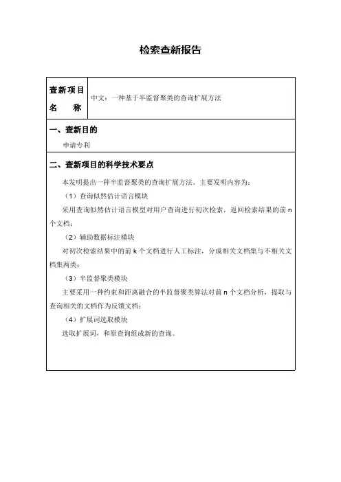
检索查新报告查新项目中文:一种基于半监督聚类的查询扩展方法名称一、查新目的申请专利二、查新项目的科学技术要点本发明提出一种半监督聚类的查询扩展方法。
主要发明内容为:(1)查询似然估计语言模块采用查询似然估计语言模型对用户查询进行初次检索,返回检索结果的前n 个文档;(2)辅助数据标注模块对初次检索结果中的前k个文档进行人工标注,分成相关文档集与不相关文档集两类;(3)半监督聚类模块主要采用一种约束和距离融合的半监督聚类算法对前n个文档分析,提取与查询相关的文档作为反馈文档;(4)扩展词选取模块选取扩展词,和原查询组成新的查询。
三、文献检索范围及检索策略(一)检索数据库:1.中国专利数据库1985—2013KI1979—20133.美国专利数据库2001—2013(二)中文检索词(英文检索词):1.半监督聚类(semi-supervised clustering)/机器学习(machine learning)2.查询扩展(query expansion)/查询优化(query optimization)/伪相关反馈(pseudo-relevance feedback)/假设相关反馈(pseudo-relevance feedback)(三)检索式或检索策略:1.(半监督聚类or机器学习)and(查询扩展or查询优化or伪相关反馈or 假设相关反馈)2.(semi-supervised clustering or machine learning)and(query expansion or query optimization or pseudo-relevance feedback)四、检索结果依据上述文献检索范围和检索式,共检索出中文相关文献8篇,列表如下:1.王秉卿.基于机器学习的查询优化研究[D].复旦大学,2012.2.黄屹.基于自学习的社会关系抽取的研究[D].北京理工大学,2011.3.叶正.基于网络挖掘与机器学习技术的相关反馈研究[D].大连理工大学,2011. 4.万涛.基于查询词聚类的信息检索系统排序模型[D].天津大学,2009.5.王秉卿,张奇,吴立德等.机器学习的查询扩展在博客检索中的应用[J].中文信息学报,2008,22(6):98-102.6.胡佳妮.文本挖掘中若干关键问题的研究[D].北京邮电大学,2008.7.王树梅.信息检索相关技术研究[D].南京理工大学,2007.8.李智,李敏强.基金项目评审管理中智能交互式文档检索[J].研究与发展管理,2005,17(3):106-110.五、查新结论相关文献对比分析如下:文献1通过采用受约束聚类对伪相关文档集合分析,找到与查询相关的文档;本发明通过采用半监督聚类(一种融合约束和距离的聚类方法)对伪相关文档集合进行分析,找到与查询相关的文档。
Large-Scale Machine Learning and GraphsCarlos GuestrinNovember 15, 2013© 2013 , Inc. and its affiliates. All rights reserved. May not be copied, modified, or distributed in whole or in part without the express consent of , Inc.PHASE 1: POSSIBILITYPHASE 2: SCALABILITYPHASE 3: USABILITYThree Phases in Technological DevelopmentWideAdoptionBeyondExperts & Enthusiast 3. Usability2. Scalability 1. PossibilityMachine Learning PHASE 1: POSSIBILITYRosenblatt 1957Machine Learning PHASE 2: SCALABILITYNeedless to Say, We Need Machine Learning for Big Data72 Hours a MinuteYouTube 28 Million Wikipedia Pages1 BillionFacebook Users 6 Billion Flickr Photos “… data a new class of economicasset, like currency or gold.”Big LearningHow will we design and implement parallel learning systems?MapReduce for Data-Parallel ML Excellent for large data-parallel tasks! Data-Parallel Graph-Parallel Cross ValidationFeatureExtraction MapReduceComputing Sufficient Statistics Is there more to Machine Learning ?The Power of Dependencies where the value is!Flashback to 1998It’s all about the graphs…Social MediaScienceAdvertisingWeb•Graphs encode the relationships between:People– –FactsProductsInterestsIdeas• Big: 100 billions of vertices and edges and rich metadataFacebook (10/2012): 1B users, 144B friendships Twitter (2011): 15B follower edgesExamples of Graphs in Machine LearningLabel a Face and PropagatePairwise similarity not enough…Not similar enough to be surePropagate Similarities & Co-occurrences for Accurate PredictionsProbabilistic Graphical Modelsco-occurring faces further evidencesimilarity edgesCollaborative Filtering: Exploiting DependenciesWomen on the Verge of a Nervous BreakdownThe CelebrationLatent Factor Models City of God Non-negative Matrix FactorizationWhat do I recommend???Wild Strawberries La Dolce VitaEstimate Political Bias?? ?Liberal? ? ?Post? ?Conservative??Post? ?? ?Semi-Supervised & ? Post Post Transductive Learning Post Post ?Post?PostPost? ?Post?Post?Post? ?PostPost???Post?Post???Topic ModelingCatApple Growth Hat PlantLDA and co.Machine Learning PipelineExtract Features Graph Formation Structured Machine Learning Algorithm Value from DataFace labels images docs Movie ratings Social activity Doc topics movie recommendDatasentiment analysisML Tasks Beyond Data-ParallelismData-Parallel Graph-ParallelCross ValidationFeature ExtractionMap ReduceComputing SufficientStatisticsGraphical Models Gibbs Sampling Belief Propagation Variational Opt.Semi-Supervised LearningLabel PropagationCoEM Graph AnalysisPageRankTriangle CountingCollaborative FilteringTensor FactorizationAlgorithmPageRankWhat’s the rankof this user?Rank?Depends on rankof who follows herDepends on rankof who follows them…Loops in graph Must iterate!PageRank Iteration–α is the random reset probability–w ji is the prob. transitioning (similarity) from j to iR[i]R[j]w jiIterate until convergence:“My rank is weightedaverage of my friends’ ranks”Properties of Graph Parallel Algorithms DependencyGraphIterativeComputationMy RankFriends RankLocalUpdatesThe Need for a New AbstractionData-Parallel Graph-ParallelCross ValidationFeature ExtractionMap ReduceComputing SufficientStatisticsGraphical Models Gibbs Sampling Belief Propagation Variational Opt.Semi-Supervised LearningLabel PropagationCoEMData-MiningPageRank Triangle CountingCollaborative FilteringTensor Factorization•Need: Asynchronous, Dynamic Parallel ComputationsThe GraphLab GoalsEfficientparallelpredictions Know how tosolve ML problemon 1 machinePOSSIBILITYData GraphData associated with vertices and edgesVertex Data:• User profile text• Current interests estimatesEdge Data:• Similarity weightsGraph:• Social NetworkHow do we program graph computation? “Think like a Vertex.” -Malewicz et al. [SIGMOD’10]pagerank(i, scope){// Get Neighborhood data(R[i], w ij, R[j]) scope;// Update the vertex data// Reschedule Neighbors if neededif R[i] changes thenreschedule_neighbors_of(i);}R[i]¬a+(1-a)wji´R[j]jÎN[i]å; Update FunctionsUser-defined program: applied tovertex transforms data in scopeDynamiccomputation Update function applied (asynchronously) in parallel until convergenceMany schedulers available to prioritize computationThe GraphLab FrameworkSchedulerConsistencyModel Graph BasedData RepresentationUpdate FunctionsUser ComputationBayesian Tensor FactorizationGibbs Sampling Dynamic Block Gibbs SamplingMatrixFactorizationLassoSVMBelief PropagationPageRank CoEMK-MeansSVDLDA…Many others…Linear SolversSplash Sampler Alternating LeastSquaresNever Ending Learner Project (CoEM) Hadoop 95 Cores 7.5 hrs32 EC2 machines 80 secs DistributedGraphLab0.3% of Hadoop time2 orders of mag faster2 orders of mag cheaper–ML algorithms as vertex programs–Asynchronous execution and consistency modelsThus far…GraphLab 1 provided exciting scaling performanceBut…We couldn’t scale up to Altavista Webgraph 20021.4B vertices, 6.7B edgesProblem:Existing distributed graph computation systems perform poorly on Natural GraphsAchilles Heel: Idealized Graph Assumption Assumed…But, Natural Graphs…Many high degree vertices(power-law degree distribution)→Very hard to partition Small degree →Easy to partitionPower-Law Degree Distribution1001021041061081010210410610810degreec o u n t High-Degree Vertices:1% vertices adjacent to50% of edgesN u m b e r o f V e r t i c e sAltaVista WebGraph1.4B Vertices, 6.6B EdgesDegree。
第19章半监督学习第3章介绍了半监督学习的概念。
它的训练样本中只有少量带有标签值,算法要解决的核心问题是如何有效的利用无标签的样本进行训练。
本质上,半监督学习也是要解决有监督学习所处理的问题。
实践结果证明,使用大量无标签样本,配合少量有标签样本,可以有效提高算法的精度。
在有些实际应用中,样本的获取成本不高,但标注成本非常高,这类问题适合使用半监督学习算法。
有监督学习中一般假设样本独立同分布。
从样本空间中抽取l个样本用于训练,他们带有标签值。
另外从样本空间中抽取u个样本,它们没有标签值。
半监督学习[1][4]要利用这些数据进行训练,得到比只用l个样本更好的效果。
19.1问题假设要利用无标签样本进行训练,必须对样本的分布进行假设。
例如对于人脸识别问题,如果一个未标注的人脸图像属于某一个人,则它和已标注的样本一样要服从某种分布,即符合这个人的特点。
半监督学习算法根据此假设来使用未标注样本,下面介绍常用的假设。
19.1.1连续性假设在数学中连续性指自变量的微小改变不会导致函数值的大幅度改变。
这里的连续性假设利用了同样的思想,距离近的样本具有相同的标签值,这是符合常规的一条假设。
在有监督学习中也使用了这一假设,如k近邻算法假设一个样本和它的邻居点有相同的类型。
19.1.2聚类假设这一假设的定义是:样本点形成一些离散的簇,同一个簇中的样本更可能是同一种类型的。
需要注意的是同一个类型的样本可能分布在多个簇中。
19.1.3流形假设这和第7章介绍的形降维算法中提出的假设相同,样本在高维空间中的分布近似位于低维空间的流形上。
在这种情况下,可以用有标签和无标签的样本学习这个流形。
19.1.4低密度分割假设对于分类问题,这里假设决策边界位于样本空间的低密度区域,即两个不同类之间的边界区域的样本稀疏。
19.2启发式算法启发式算法是最简单的半监督学习算法,它的核心思想是先用有标签样本进行训练,然后用训练得到的模型对无标签样本进行预测,从中挑选出一部分样本继续进行训练,以提升模型的精度。
人工智能常见算法简介人工智能的三大基石—算法、数据和计算能力,算法作为其中之一,是非常重要的,那么人工智能都会涉及哪些算法呢?不同算法适用于哪些场景呢?一、按照模型训练方式不同可以分为监督学习(Supervised Learning),无监督学习(Unsupervised Learning)、半监督学习(Semi-supervised Learning)和强化学习(Reinforcement Learning)四大类。
常见的监督学习算法包含以下几类:(1)人工神经网络(Artificial Neural Network)类:反向传播(Backpropagation)、波尔兹曼机(Boltzmann Machine)、卷积神经网络(Convolutional Neural Network)、Hopfield网络(hopfield Network)、多层感知器(Multilyer Perceptron)、径向基函数网络(Radial Basis Function Network,RBFN)、受限波尔兹曼机(Restricted Boltzmann Machine)、回归神经网络(Recurrent Neural Network,RNN)、自组织映射(Self-organizing Map,SOM)、尖峰神经网络(Spiking Neural Network)等。
(2)贝叶斯类(Bayesin):朴素贝叶斯(Naive Bayes)、高斯贝叶斯(Gaussian Naive Bayes)、多项朴素贝叶斯(Multinomial Naive Bayes)、平均-依赖性评估(Averaged One-Dependence Estimators,AODE)贝叶斯信念网络(Bayesian Belief Network,BBN)、贝叶斯网络(Bayesian Network,BN)等。
(3)决策树(Decision Tree)类:分类和回归树(Classification and Regression Tree,CART)、迭代Dichotomiser3(Iterative Dichotomiser 3, ID3),C4.5算法(C4.5 Algorithm)、C5.0算法(C5.0 Algorithm)、卡方自动交互检测(Chi-squared Automatic Interaction Detection,CHAID)、决策残端(Decision Stump)、ID3算法(ID3 Algorithm)、随机森林(Random Forest)、SLIQ(Supervised Learning in Quest)等。
三、机器学习的分类三 -- Types of Learning上节课我们主要介绍了解决线性分类问题的⼀个简单的⽅法:PLA。
PLA能够在平⾯中选择⼀条直线将样本数据完全正确分类。
⽽对于线性不可分的情况,可以使⽤Pocket Algorithm来处理。
本节课将主要介绍⼀下机器学习有哪些种类,并进⾏归纳。
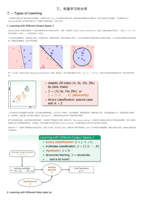
1. Learning with Different Output Space Y我们在上节课引⼊的银⾏根据⽤户个⼈情况判断是否给他发信⽤卡的例⼦,这是⼀个典型的⼆元分类(binary classification)问题。
也就是说输出只有两个,⼀般y={-1, +1},-1代表不发信⽤卡(负类),+1代表发信⽤卡(正类)。
⼆元分类的问题很常见,包括信⽤卡发放、垃圾邮件判别、患者疾病诊断、答案正确性估计等等。
⼆元分类是机器学习领域⾮常核⼼和基本的问题。
⼆元分类有线性模型也有⾮线性模型,根据实际问题情况,选择不同的模型。
除了⼆元分类,也有多元分类(Multiclass Classification)问题。
顾名思义,多元分类的输出多于两个,y={1, 2, … , K}, K>2. ⼀般多元分类的应⽤有数字识别、图⽚内容识别等等。
⼆元分类和多元分类都属于分类问题,它们的输出都是离散值。
⼆对于另外⼀种情况,⽐如训练模型,预测房屋价格、股票收益多少等,这类问题的输出y=R,即范围在整个实数空间,是连续的。
这类问题,我们把它叫做回归(Regression)。
最简单的线性回归是⼀种典型的回归模型。
除了分类和回归问题,在⾃然语⾔处理等领域中,还会⽤到⼀种机器学习问题:结构化学习(Structured Learning)。
结构化学习的输出空间包含了某种结构在⾥⾯,它的⼀些解法通常是从多分类问题延伸⽽来的,⽐较复杂。
本系列课程不会详细介绍Structured Learning,有兴趣的读者可以⾃⾏对它进⾏更深⼊的研究。
MachLearn(2009)74:1–22DOI10.1007/s10994-008-5084-4
Semi-supervisedgraphclustering:akernelapproachBrianKulis·SugatoBasu·InderjitDhillon·RaymondMooney
Received:9March2007/Revised:17April2008/Accepted:8August2008/Publishedonline:24September2008SpringerScience+BusinessMedia,LLC2008
AbstractSemi-supervisedclusteringalgorithmsaimtoimproveclusteringresultsusinglimitedsupervision.Thesupervisionisgenerallygivenaspairwiseconstraints;suchcon-straintsarenaturalforgraphs,yetmostsemi-supervisedclusteringalgorithmsaredesignedfordatarepresentedasvectors.Inthispaper,weunifyvector-basedandgraph-basedap-proaches.Wefirstshowthatarecently-proposedobjectivefunctionforsemi-supervisedclusteringbasedonHiddenMarkovRandomFields,withsquaredEuclideandistanceandacertainclassofconstraintpenaltyfunctions,canbeexpressedasaspecialcaseoftheweightedkernelk-meansobjective(Dhillonetal.,inProceedingsofthe10thInternationalConferenceonKnowledgeDiscoveryandDataMining,2004a).Arecenttheoreticalcon-nectionbetweenweightedkernelk-meansandseveralgraphclusteringobjectivesenablesustoperformsemi-supervisedclusteringofdatagiveneitherasvectorsorasagraph.Forgraphdata,thisresultleadstoalgorithmsforoptimizingseveralnewsemi-supervisedgraphclusteringobjectives.Forvectordata,thekernelapproachalsoenablesustofindclusterswithnon-linearboundariesintheinputdataspace.Furthermore,weshowthatrecentworkonspectrallearning(Kamvaretal.,inProceedingsofthe17thInternationalJointConfer-enceonArtificialIntelligence,2003)maybeviewedasaspecialcaseofourformulation.Weempiricallyshowthatouralgorithmisabletooutperformcurrentstate-of-the-artsemi-supervisedalgorithmsonbothvector-basedandgraph-baseddatasets.
KeywordsSemi-supervisedclustering·Kernelk-means·Graphclustering·Spectrallearning
Editor:JenniferDy.B.Kulis()·I.Dhillon·R.MooneyDepartmentofComputerSciences,UniversityofTexas,Austin,TX,USAe-mail:kulis@cs.utexas.edu
S.BasuGoogle,Inc.,MountainView,CA,USA2MachLearn(2009)74:1–221IntroductionSemi-supervisedclusteringalgorithmshaverecentlyreceivedasignificantamountofatten-tioninthemachinelearninganddataminingcommunities.Intraditionalclusteringalgo-rithms,onlyunlabeleddataisusedtogenerateclusterings;insemi-supervisedclustering,thegoalistoincorporatepriorinformationaboutclustersintothealgorithminordertoimprovetheclusteringresults.Arelatedbutdifferentproblemissemi-supervisedclassi-fication(Chapelleetal.2006),whichconsidershowunlabeleddatacanbeusedtoim-provetheperformanceofclassificationonlabeleddata.Anumberofrecentpapershaveexploredtheproblemofsemi-supervisedclustering.Researchonsemi-supervisedcluster-inghasconsideredsupervisionintheformofbothlabeledpoints(Demirizetal.1999;SinkkonenandKaski2002;Basuetal.2002)orconstraints(Wagstaffetal.2001;Kleinetal.2002;Xingetal.2003;Bar-Hilleletal.2003;Bieetal.2003;Kamvaretal.2003;Bilenkoetal.2004;Basuetal.2004a,2004b;ChangandYeung2004;DavidsonandRavi2005a,2005b;Lawetal.2005;LuandLeen2005;Langeetal.2005).Asiscommonformostsemi-supervisedclusteringalgorithms,weassumeinthispaperthatwehavepairwisemust-linkconstraints(pairsofpointsthatshouldbelonginthesamecluster)andcannot-linkconstraints(pairsofpointsthatshouldbelongindifferentclus-ters)providedwiththeinput.Pairwiseconstraintsoccurnaturallyinmanydomains,e.g.,theDatabaseofInteractingProteins(DIP)datasetinbiologycontainsinformationaboutproteinsco-occurringinprocesses,whichcanbeviewedasmust-linkconstraintsduringgeneclustering.Constraintsofthisformarealsonaturalinthecontextofthegraphcluster-ingproblem(a.k.a.graphpartitioningorvertexpartitioning),whereedgesinthegraphen-codepairwiserelationships.Differentapplicationareasofsemi-supervisedclusteringwithconstraintshavebeenstudiedrecently,including(1)imagesegmentationforobjectiden-tificationinAiborobots(DavidsonandRavi2005a),wherecluster-levelconstraintsareusedtoimprovethepixelclustering;(2)objectrecognitioninvideosequences(Yanetal.2004),wheremust-linkconstraintsareusedtogrouppixelsbelongingtothesameobjectandcannot-linkconstraintsareusedtoseparatedifferentobjects;(3)clusteringforlanefindingfromGPStraces(Wagstaffetal.2001),whereconstraintsareusedtoencodelane-contiguityandmax-separationcriteria;and(4)speakeridentificationandcategorization(Bar-Hilleletal.2003),whereconstraintsareusedtoencodewhethertwospeakersaresimilarornot.Recently,aprobabilisticframeworkforsemi-supervisedclusteringwithpairwisecon-straintswasproposedbasedonHiddenMarkovRandomFields(Basuetal.2004b).TheHMRFframeworkproposedageneralsemi-supervisedclusteringobjectivebasedonmaxi-mizingthejointlikelihoodofdataandconstraintsintheHMRFmodel,aswellasak-means-likeiterativealgorithmforoptimizingtheobjective.However,HMRF-KMEANScancluster