Using Semi-Supervised Clustering to Improve Regression Test
- 格式:pdf
- 大小:300.28 KB
- 文档页数:10

I.J. Information Technology and Computer Science, 2012, 6, 12-17Published Online June 2012 in MECS (/)DOI: 10.5815/ijitcs.2012.06.02Mining the Shirt Sizes for Indian Men byClustered ClassificationM. Martin JeyasinghNational Institute of Fashion Technology, Chennai. India.Email:mmjsingh@Kumaravel AppavooBharath Institute of Higher Education and Research , Chennai -73,Tamilnadu,India.Email: drkumaravel@Abstract—In garment production engineering, sizing system plays an important role for manufacturing of clothing. The standards for defining the size label are a critical issue. Locating the right garment size for a customer depends on the label as an interface. In this research work intend to approach that it could be used for developing sizing systems by data mining techniques applied to Indian anthropometric dataset. We propose a new approach of two-stage data mining procedure for labelling the shirt types exclusively for Indian men. In the first stage , clustering technique applied on the original dataset, to categorise the size labels. Then these clusters are used for supervised learning in the second stage for classification. A sizing system classifies a specific population into homogeneous subgroups based on some key body dimensions. The space with these dimensions gives raise to complexity for finding uniform standards. This enables us to have an interface as a communication tool among manufacturers, retailers and consumers. This sizing system is developed for the men‟s age ranges between 25 and 66 years. Main attribute happens to be the chest size as clearly visible in the data set. We have obtained classifications for men‟s shirt attributes based on clustering techniques.Index Terms—Data Mining ,Clustering, Classifiers, IBK KNN, Logitboost, Clothing industry, Anthropometric data.I.IntroductionGarment sizing systems were originally based on those developed by tailors in the late 18th century. Professional dressmakers and craftsmen were developed various sizing methods in the past years. They used unique techniques for measuring and fitting their customers. In the 1920s, the demand for the mass production of garments created the need for a standard sizing system. Many researchers started working on developing sizing system by the different methods and data collecting approaches. It has proved that garment manufacturing is the highest value-added industry in textile industry manufacturing cycle [1]. Mass production by machines in this industry has replaced manual manufacturing, so the planning and quality control of production and inventory are very important for manufacturer. Moreover, this type of manufacturing has demand to certain standards and specifications. Furthermore each country has its own standard sizing systems for manufacturers to follow and fit in with the figure types of the local population.A sizing system classifies a specific population into homogeneous subgroups based on some key body dimensions [2]. Persons of the same subgroup have the garment size. Standard sizing systems can correctly predict manufacturing quantity and proportion of production, resulting more accurate production planning and control of materials [3, 4]. The standard unique techniques for measuring and fitting their sizing systems have been used as a communication tool among manufacturers, retailers and consumers.It can provide manufacturers with size specification, design development, pattern grading and market analysis. Manufacturers, basing their judgments on the information, can produce different type of garments with the various allowances for specific market segmentation. Thus, establishing standard sizing systems are necessary and important. Many researchers worked on developing the sizing system are necessary and important by many approaches. They found very extensive data were made by using anthropometric data [2].People have changed in body shape over time. Workman [5] demonstrated that the problem of ageing contributes to the observed changes in body shape and size, more than any other single factor, such as improved diet and longer life expectancy [6]. Sizing concerns will grow as the number of ageing consumers is expected to double by the year 2030. This presents a marketing challenge for the clothing industry since poor sizing is the number one reason for returns and markdowns, resulting in substantial losses. Therefore, sizing systems have to be updated from time to time in order to ensure the correct fit of ready-to-wear apparel. Many countries have been undertaking sizing surveys in recent years. Since sizing practices vary fromcountry to country, in 1968 Sweden originated the first official approach to the International Organization for Standardization (ISO) on the subject of sizing of clothing, it being in the interest of the general public that an international system be created. After lengthy discussions and many proposals, members of technical committee TC133 submitted documents relating to secondary body dimensions, their definitions and methods of measuring. This eventually resulted in the publication of ISO 8559 …Garment Constructio n and Anthropometric Surveys - Body Dimension, which is currently used as an international standard for all types of size survey [7].Figure type plays a decisive role in a sizing system and contributes to the topic of fit. So to find a sizing system, different body types are first divided from population, based on dimensions, such as height or ratios between body measurements. A set of size categories is developed, each containing a range of sizes from small to large. The size range is generally evenly distributed from the smallest to the largest size in the most countries. For men's wear, the body length and drop value are the two main measurements characterizing the definition of figure type. Bureau of Indian Standards (BIS) identified three body heights; short (166 cm), regular (174 cm) and tall (182 cm) [20] recommended the use of the difference in figure types as the classification of ready-to-wears and developed a set of procedures to formulate standard sizes for all figure types. In early times, the classification of figure types was based on body weight and stature. Later on, anthropometric dimensions were applied for classification. This type of sizing system has the advantages of easy grading and size labeling. But, the disadvantage is that the structural constraints in the linear system may result in a loose fit. Thus, some optimization methods have been proposed to generate a better fit sizing system, such as an integer programming approach [10] and a nonlinear programming approach [11]. For the development of sizing systems using optimization methods, the structure of the sizing systems tends to affect the predefined constraints and objectives. Tryfos [10] indicated that the probability of purchase depended on the distance between the sizing system of a garment and the real size of an individual. In order to optimize the number of sizes so as to minimize the distance, an integer programming approach was applied to choose the optimal sizes. Later on, McCulloch, et al. [11] constructed a sizing system by using a nonlinear optimization approach to maximize the quality of fit. Recently, Gupta, et al. [12] used a linear programming approach to classify the size groups. Using the optimization method has the advantages of generating a sizing system with an optimal fit, but the irregular distribution of the optimal sizes may increase the complexity in grading and the cost of production. On the other hand, in recent years, data mining has been widely used in area of science and engineering. The application domain is quite broad and plausible in bioinformatics, genetics, medicine, education, electrical power engineering, marketing, production, human resource management, risk prediction, biomedical technology and health insurance. In the field of sizing system in clothing science, data mining techniques such as neural networks [13], cluster analysis [14], the decision tree approach [15] and two stage cluster analysis [16] have been used. Clustering is the classification of objects into different groups, or more precisely, the partitioning of a data set into subsets (clusters), so that the data in each subset (ideally) share some common trait. Cluster analysis was used as an exploratory data analysis tool for classification. In the clothing a cluster which is typically grouped by the similarity of its members‟ shirt sizes can grouped by the K-means cluster analysis method to classify the upper garment sizing system. The pitfall of these methods is that it requires one to pre-assign the number of clusters to initialize the algorithm and it is usually subjectively determined by experts. To overcome these disadvantages, a two stage-based data mining procedure include cluster analysis and classification algorithms, is proposed here to eliminate the requirement of subjective judgment and to improve the effectiveness of size classification[8]. II.Data Mining Techniques2.1. Data PreparationAfter the definition of industry problem, first stage of data mining, data preparation selected to increase the efficiency and ensure the accuracy of its analysis through the processing and transformation of the data. Before starting to mine the data, they must be examined and proceed with all missing data and outliers. By examining the data before the application of a multivariate technique, the researcher gains several critical insights into the characteristics of the data. In this research work, we used an anthropometric database which was collected from BIS and from Clothing industrialists. Anthropometric data of 620 Indian men with the age ranged from 25 to 66 years from the database were obtained. The data mining process as shown Fig.1.2.2. Cluster Analysis:First step of data mining approach was undertaken, X‟Means clustering in the cluster analysis. X-Means is K-Means extended by an improve-structure part, In this part of the algorithm the centers are attempted to be split in its region. The decision between the children of each center and itself is done comparing the BIC-values of the two structures. With the difference between the age and the other attributes, we determined the cluster numbers. In the cluster analysis, K-means method implemented to determine the final cluster categorization.Fig. 1 Data mining process2.3.Classification Techniques2.3.1. K-nearest neighbourK-nearest neighbour algorithm (K-nn) is a supervised learning algorithm that has been used in many applications in the field of data mining, statistical pattern recognition, image processing and many others. K-nn is a method for classifying objects based on closest training examples in the feature space. The k-neighbourhood parameter is determined in the initialization stage of K-nn. The k samples which are closest to new sample are found among the training data. The class of the new sample is determined according to the closest k-samples by using majority voting [9]. Distance measurements like Euclidean, Hamming and Manhattan are used to calculate the distances of the samples to each other.2.3.2. Random TreeIn this classifier the class for constructing a tree that considers K randomly chosen attributes at each node. It performs no pruning. Also has an option to allow estimation of class probabilities based on a hold-out set (back fitting). Sets the number of randomly chosen attributes by K Value. To allow the unclassified instances, maximum depth of the tree, the minimum total weight of the instances in a leaf and the random number seed used for selecting attributes could parameterised, numFolds -- Determines the amount of data used for back fitting and one fold is used for back fitting, the rest for growing the tree. (Default: 0, no back fitting) .2.3.3.LogitboostIn this classifier the class for performing additive logistic regression. This class performs classification using a regression scheme as the base learner, and can handle multi-class problems. Can do efficient internal cross-validation to determine appropriate number of iterations. This classifier may output additional infomation to the console, threshold on improvement in likelihood, the number of iterations to be performed, number of runs for internal cross-validation, weight threshold for weight pruning (reduce to 90 for speeding up learning process) are parameterised, numFolds -- number of folds for internal cross-validation (default 0 means no cross-validation is performed) to be specified. III.Data description3.1. Description of DatasetData processing : The data types like nominal(text), numeric or the missing data has been filled with meaningful assumptions in the database. Database specification with description and table structure as shown in Table 1.TABLE 1. SPECIFICATION OF DATABASE3.3. The Application of Data MiningData mining could be used to uncover patterns. The increasing power of computer technology has increased data collection and storage. Automatic data processing has been aided by computer science, such as neural networks, clustering, genetic algorithms, decision trees, Digital printing and support vector machines. Data mining is the process of applying these methods to the prediction of uncovering hidden patterns [18]. It has been used for many years by businesses, scientists to sift through volumes of data. The application of data mining in fashion product development for production detect and forecasting analysis by using classification and clustering methods as shown in Fig. 2.Fig.2 . Application of data mining in Fashion IndustryIV. Experimental Results4.1.Distribution of ClassesThis dataset has different characteristics such as: the number of attributes, the number of classes, the number of records and the percentage of class occurrences. Like the test dataset, 620 different types of shirt sizes are broadly categorized in six groups as XS, S, M, L, XL,XXL. The Distribution of Classes in the actual training data for classifiers evaluation and the occurrences as given in Table II. The percentage of size Categories using Pie chart as shown in Fig.3 and after clustered size categories shown in Fig.4.TABLE II DISTRIBUTION OF CLASSES IN THE ACTUALTRAINING SETFig.3. Percentage of size CategoriesFig.4. Percentage of size Categories after clustered4.2. Experimental OutcomesTo estimate the performance of the cluster method, we compared the results generated by cluster with the results generated by original sets of attributes for the chosen dataset. In the experiments, the data mining software called weka 3.6.4 which has been implemented in Java with latest windows 7 operating system in Intel Core2Quad@2.83 GHz processor and 2 GB memory, These dataset has been applied and then evaluated for accuracy by using 10-fold Cross Validation strategy [19]. The predicted result values of various classifiers with prediction accuracy as given Table III.The dataset with original features and clustered form of the dataset are classified with the algorithms K-nn[17] with 5 neighbours, Random tree, Logitboost without pruning. Both of the obtained classification results are compared. In each phase of a cross validation, one of the yet unprocessed sets was tested, while the union of all remaining sets was used as training set for classification by the above algorithms. Classifiers with prediction accuracy and difference is given in Table III. Performance of the classifiers as shown in Fig.5. Difference between original and clustered classification accuracy rate has been shown in Fig.6.14%13% 19%19%15%20%Percentage of Size CategoriesXS S ML XL XXL9%7%15%22%7%40%Percentage of Size Categories afterClusteredXS S ML XL XXLTABLE III . CLASSIFIERS WITH PREDICTION ACCURACYFig.5. Performance of classifiersparision between Original Clustered accuracy V.ConclusionIn this research work, Cluster classification method is used to improve and achieve the shirt size grouping by classification accuracy. In the first phase, the dataset has been clustered to acquire the system defined size grouping by clustering. Second phase, we experimented the performance of this approach with the popular algorithms such as K-nn, Jrip, Random tree, decision table, Multilayerperceptron. When one searches for higher accuracy, IBK Knn-4 performance highest among all the other algorithms by comparing the original and clustered classification accuracy rate. References[1]Chang, C.F., 1999. “The model analysis of femalebody size measurement from 18 to 22, J. HwaGang Textile, 6: 86-94.[2]Fan, J., W. Yu and H. Lawrance, 2004. Clothingappearance and fit: Science and technology,Woodhead Publishing Limited, Cambridge,England.[3]Tung, Y.M. and S.S. Soong, 1994. The demandside analysis for Taiwan domestic apparel market,J. the China Textile Institute, 4: 375-380.[4]Hsu, K.M. and S.H. Jing, 1999. The chances ofTaiwan apparel industry, J. the China TextileInstitute, 9: 1-6.[5]Workman, J.E., 1991. Body measurementspecification for fit models as a factor in apparelsize variation, Cloth Text Res. J., 10(1): 31-36.[6]LaBat, K.L. and M.R. Delong, 1990. Bodycathexis and satisfaction with fit of apparel, ClothText Res. J., 8(2): 42-48.[7]ISO 8559, 1989. Garment Construction andAnthropometric Surveys - Body Dimensions,International Organization for Standardization.[8]R.Bagherzadeh,tifi and A.R.Faramarzi,2010,Employing a Three-Stage Data MiningProcedure to Develop Sizing System, WorldApplied Sciences Journal 8 (8): 923-929.[9]G.Shakhnarovish,T. Darrell and P. Indyk, 2005,“Nearest Neighbor Methods in Learning andVision,”MIT Press, Informatics, vol. 37, no. 6,December, 2004, pp. 461-470[10]Tryfos, P., 1986. An integer programmingapproach to the apparel sizing problem, J. theOperational Research Society, 37(10): 1001-1006[11]McCulloch, C.E., B. Paal and S.A. Ashdown,1998. An optimal approach to apparel sizing, J.the Operational Res. Society, 49: 492-499.[12]Gupta, D., N. Garg, K. Arora and N. Priyadarshini,2006. Developing body measurement charts forgarments manufacture based on a linearprogramming approach, J. Textile and ApparelTechnology and Management, 5(1): 1-13.[13]She, F.H., L.X. Kong, S. Nahavandi and A.Z.Kouzani, 2002. Intelligent animal fiberclassification with artificial neural networks,Textile Research J., 72(7): 594-600.[14]Moon, J.Y. and Y.N. Nam, 2003. A study theelderly women‟s lower body type classificationand lower garment sizing systems, Proceedings ofInternational Ergonomics Association Conference.[15]Hsu, C.H. and M.J. Wang, 2005. Using decisiontree based data mining to establish a sizing systemfor the manufacture of garments, International J.Advanced Manufacturing Technol., 26(5& 6):669-674.[16]Meng, J.C., L. Hai and J.J.W. Mao, 2007.Thedevelopment of sizing systems for Taiwaneseelementary- and high-school students,International J. Industrial Ergonomics, 37: 707-716.[17]J. R.Quinlan, 1993, “C4.5: Programs for machinelearning,” San Francisco, CA: Morgan Kaufman.[18]Liang Xun, 2006,Data Mining:Algorithms andApplication. Beijing university Press: pp.22-42. [19]Stephan White, 2004, Enhancing the academiclearning opportunities for all students. Such aplan Examination of the Meta-Analytic Evidence,in School Desegregation .. at 68, 68–72;.[20]Bureau of Indian Standards(BIS),Indian standardsize designation of clothes definition and bodymeasurement procedure,ICS 61.020,IS14453:1997.[21]Winifred Aldrich,2008,Metric Pattern cutting forMenswear,Fourth Edition, Blackwell publishing,ISBN-978 1405 10278 0,10-15.M. Martin Jeyasingh:Associate Professor, National Institute of Fashion Technology, Chennai-119.India. Kumaravel Appavoo: Dean & Professor, Department of Computer Science,Bharath Institute of Higher Education and Research , Chennai -73,Tamilnadu,India。
常用英语词汇 -andrew Ng课程average firing rate均匀激活率intensity强度average sum-of-squares error均方差Regression回归backpropagation后向流传Loss function损失函数basis 基non-convex非凸函数basis feature vectors特点基向量neural network神经网络batch gradient ascent批量梯度上涨法supervised learning监察学习Bayesian regularization method贝叶斯规则化方法regression problem回归问题办理的是连续的问题Bernoulli random variable伯努利随机变量classification problem分类问题bias term偏置项discreet value失散值binary classfication二元分类support vector machines支持向量机class labels种类标记learning theory学习理论concatenation级联learning algorithms学习算法conjugate gradient共轭梯度unsupervised learning无监察学习contiguous groups联通地区gradient descent梯度降落convex optimization software凸优化软件linear regression线性回归convolution卷积Neural Network神经网络cost function代价函数gradient descent梯度降落covariance matrix协方差矩阵normal equations DC component直流重量linear algebra线性代数decorrelation去有关superscript上标degeneracy退化exponentiation指数demensionality reduction降维training set训练会合derivative导函数training example训练样本diagonal对角线hypothesis假定,用来表示学习算法的输出diffusion of gradients梯度的弥散LMS algorithm “least mean squares最小二乘法算eigenvalue特点值法eigenvector特点向量batch gradient descent批量梯度降落error term残差constantly gradient descent随机梯度降落feature matrix特点矩阵iterative algorithm迭代算法feature standardization特点标准化partial derivative偏导数feedforward architectures前馈构造算法contour等高线feedforward neural network前馈神经网络quadratic function二元函数feedforward pass前馈传导locally weighted regression局部加权回归fine-tuned微调underfitting欠拟合first-order feature一阶特点overfitting过拟合forward pass前向传导non-parametric learning algorithms无参数学习算forward propagation前向流传法Gaussian prior高斯先验概率parametric learning algorithm参数学习算法generative model生成模型activation激活值gradient descent梯度降落activation function激活函数Greedy layer-wise training逐层贪心训练方法additive noise加性噪声grouping matrix分组矩阵autoencoder自编码器Hadamard product阿达马乘积Autoencoders自编码算法Hessian matrix Hessian矩阵hidden layer隐含层hidden units隐蔽神经元Hierarchical grouping层次型分组higher-order features更高阶特点highly non-convex optimization problem高度非凸的优化问题histogram直方图hyperbolic tangent双曲正切函数hypothesis估值,假定identity activation function恒等激励函数IID 独立同散布illumination照明inactive克制independent component analysis独立成份剖析input domains输入域input layer输入层intensity亮度/灰度intercept term截距KL divergence相对熵KL divergence KL分别度k-Means K-均值learning rate学习速率least squares最小二乘法linear correspondence线性响应linear superposition线性叠加line-search algorithm线搜寻算法local mean subtraction局部均值消减local optima局部最优解logistic regression逻辑回归loss function损失函数low-pass filtering低通滤波magnitude幅值MAP 极大后验预计maximum likelihood estimation极大似然预计mean 均匀值MFCC Mel 倒频系数multi-class classification多元分类neural networks神经网络neuron 神经元Newton’s method牛顿法non-convex function非凸函数non-linear feature非线性特点norm 范式norm bounded有界范数norm constrained范数拘束normalization归一化numerical roundoff errors数值舍入偏差numerically checking数值查验numerically reliable数值计算上稳固object detection物体检测objective function目标函数off-by-one error缺位错误orthogonalization正交化output layer输出层overall cost function整体代价函数over-complete basis超齐备基over-fitting过拟合parts of objects目标的零件part-whole decompostion部分-整体分解PCA 主元剖析penalty term处罚因子per-example mean subtraction逐样本均值消减pooling池化pretrain预训练principal components analysis主成份剖析quadratic constraints二次拘束RBMs 受限 Boltzman 机reconstruction based models鉴于重构的模型reconstruction cost重修代价reconstruction term重构项redundant冗余reflection matrix反射矩阵regularization正则化regularization term正则化项rescaling缩放robust 鲁棒性run 行程second-order feature二阶特点sigmoid activation function S型激励函数significant digits有效数字singular value奇怪值singular vector奇怪向量smoothed L1 penalty光滑的L1 范数处罚Smoothed topographic L1 sparsity penalty光滑地形L1 稀少处罚函数smoothing光滑Softmax Regresson Softmax回归sorted in decreasing order降序摆列source features源特点Adversarial Networks抗衡网络sparse autoencoder消减归一化Affine Layer仿射层Sparsity稀少性Affinity matrix亲和矩阵sparsity parameter稀少性参数Agent 代理 /智能体sparsity penalty稀少处罚Algorithm 算法square function平方函数Alpha- beta pruningα - β剪枝squared-error方差Anomaly detection异样检测stationary安稳性(不变性)Approximation近似stationary stochastic process安稳随机过程Area Under ROC Curve/ AUC Roc 曲线下边积step-size步长值Artificial General Intelligence/AGI通用人工智supervised learning监察学习能symmetric positive semi-definite matrix Artificial Intelligence/AI人工智能对称半正定矩阵Association analysis关系剖析symmetry breaking对称无效Attention mechanism注意力体制tanh function双曲正切函数Attribute conditional independence assumptionthe average activation均匀活跃度属性条件独立性假定the derivative checking method梯度考证方法Attribute space属性空间the empirical distribution经验散布函数Attribute value属性值the energy function能量函数Autoencoder自编码器the Lagrange dual拉格朗日对偶函数Automatic speech recognition自动语音辨别the log likelihood对数似然函数Automatic summarization自动纲要the pixel intensity value像素灰度值Average gradient均匀梯度the rate of convergence收敛速度Average-Pooling均匀池化topographic cost term拓扑代价项Backpropagation Through Time经过时间的反向流传topographic ordered拓扑次序Backpropagation/BP反向流传transformation变换Base learner基学习器translation invariant平移不变性Base learning algorithm基学习算法trivial answer平庸解Batch Normalization/BN批量归一化under-complete basis不齐备基Bayes decision rule贝叶斯判断准则unrolling组合扩展Bayes Model Averaging/ BMA 贝叶斯模型均匀unsupervised learning无监察学习Bayes optimal classifier贝叶斯最优分类器variance 方差Bayesian decision theory贝叶斯决议论vecotrized implementation向量化实现Bayesian network贝叶斯网络vectorization矢量化Between-class scatter matrix类间散度矩阵visual cortex视觉皮层Bias 偏置 /偏差weight decay权重衰减Bias-variance decomposition偏差 - 方差分解weighted average加权均匀值Bias-Variance Dilemma偏差–方差窘境whitening白化Bi-directional Long-Short Term Memory/Bi-LSTMzero-mean均值为零双向长短期记忆Accumulated error backpropagation积累偏差逆传Binary classification二分类播Binomial test二项查验Activation Function激活函数Bi-partition二分法Adaptive Resonance Theory/ART自适应谐振理论Boltzmann machine玻尔兹曼机Addictive model加性学习Bootstrap sampling自助采样法/可重复采样Bootstrapping自助法Break-Event Point/ BEP 均衡点Calibration校准Cascade-Correlation级联有关Categorical attribute失散属性Class-conditional probability类条件概率Classification and regression tree/CART分类与回归树Classifier分类器Class-imbalance类型不均衡Closed -form闭式Cluster簇/ 类/ 集群Cluster analysis聚类剖析Clustering聚类Clustering ensemble聚类集成Co-adapting共适应Coding matrix编码矩阵COLT 国际学习理论会议Committee-based learning鉴于委员会的学习Competitive learning竞争型学习Component learner组件学习器Comprehensibility可解说性Computation Cost计算成本Computational Linguistics计算语言学Computer vision计算机视觉Concept drift观点漂移Concept Learning System /CLS观点学习系统Conditional entropy条件熵Conditional mutual information条件互信息Conditional Probability Table/ CPT 条件概率表Conditional random field/CRF条件随机场Conditional risk条件风险Confidence置信度Confusion matrix混杂矩阵Connection weight连结权Connectionism 连结主义Consistency一致性/相合性Contingency table列联表Continuous attribute连续属性Convergence收敛Conversational agent会话智能体Convex quadratic programming凸二次规划Convexity凸性Convolutional neural network/CNN卷积神经网络Co-occurrence同现Correlation coefficient有关系数Cosine similarity余弦相像度Cost curve成本曲线Cost Function成本函数Cost matrix成本矩阵Cost-sensitive成本敏感Cross entropy交错熵Cross validation交错考证Crowdsourcing众包Curse of dimensionality维数灾害Cut point截断点Cutting plane algorithm割平面法Data mining数据发掘Data set数据集Decision Boundary决议界限Decision stump决议树桩Decision tree决议树/判断树Deduction演绎Deep Belief Network深度信念网络Deep Convolutional Generative Adversarial NetworkDCGAN深度卷积生成抗衡网络Deep learning深度学习Deep neural network/DNN深度神经网络Deep Q-Learning深度Q 学习Deep Q-Network深度Q 网络Density estimation密度预计Density-based clustering密度聚类Differentiable neural computer可微分神经计算机Dimensionality reduction algorithm降维算法Directed edge有向边Disagreement measure不合胸怀Discriminative model鉴别模型Discriminator鉴别器Distance measure距离胸怀Distance metric learning距离胸怀学习Distribution散布Divergence散度Diversity measure多样性胸怀/差别性胸怀Domain adaption领域自适应Downsampling下采样D-separation( Directed separation)有向分别Dual problem对偶问题Dummy node 哑结点General Problem Solving通用问题求解Dynamic Fusion 动向交融Generalization泛化Dynamic programming动向规划Generalization error泛化偏差Eigenvalue decomposition特点值分解Generalization error bound泛化偏差上界Embedding 嵌入Generalized Lagrange function广义拉格朗日函数Emotional analysis情绪剖析Generalized linear model广义线性模型Empirical conditional entropy经验条件熵Generalized Rayleigh quotient广义瑞利商Empirical entropy经验熵Generative Adversarial Networks/GAN生成抗衡网Empirical error经验偏差络Empirical risk经验风险Generative Model生成模型End-to-End 端到端Generator生成器Energy-based model鉴于能量的模型Genetic Algorithm/GA遗传算法Ensemble learning集成学习Gibbs sampling吉布斯采样Ensemble pruning集成修剪Gini index基尼指数Error Correcting Output Codes/ ECOC纠错输出码Global minimum全局最小Error rate错误率Global Optimization全局优化Error-ambiguity decomposition偏差 - 分歧分解Gradient boosting梯度提高Euclidean distance欧氏距离Gradient Descent梯度降落Evolutionary computation演化计算Graph theory图论Expectation-Maximization希望最大化Ground-truth实情/真切Expected loss希望损失Hard margin硬间隔Exploding Gradient Problem梯度爆炸问题Hard voting硬投票Exponential loss function指数损失函数Harmonic mean 调解均匀Extreme Learning Machine/ELM超限学习机Hesse matrix海塞矩阵Factorization因子分解Hidden dynamic model隐动向模型False negative假负类Hidden layer隐蔽层False positive假正类Hidden Markov Model/HMM 隐马尔可夫模型False Positive Rate/FPR假正例率Hierarchical clustering层次聚类Feature engineering特点工程Hilbert space希尔伯特空间Feature selection特点选择Hinge loss function合页损失函数Feature vector特点向量Hold-out 留出法Featured Learning特点学习Homogeneous 同质Feedforward Neural Networks/FNN前馈神经网络Hybrid computing混杂计算Fine-tuning微调Hyperparameter超参数Flipping output翻转法Hypothesis假定Fluctuation震荡Hypothesis test假定考证Forward stagewise algorithm前向分步算法ICML 国际机器学习会议Frequentist频次主义学派Improved iterative scaling/IIS改良的迭代尺度法Full-rank matrix满秩矩阵Incremental learning增量学习Functional neuron功能神经元Independent and identically distributed/独Gain ratio增益率立同散布Game theory博弈论Independent Component Analysis/ICA独立成分剖析Gaussian kernel function高斯核函数Indicator function指示函数Gaussian Mixture Model高斯混杂模型Individual learner个体学习器Induction归纳Inductive bias归纳偏好Inductive learning归纳学习Inductive Logic Programming/ ILP归纳逻辑程序设计Information entropy信息熵Information gain信息增益Input layer输入层Insensitive loss不敏感损失Inter-cluster similarity簇间相像度International Conference for Machine Learning/ICML国际机器学习大会Intra-cluster similarity簇内相像度Intrinsic value固有值Isometric Mapping/Isomap等胸怀映照Isotonic regression平分回归Iterative Dichotomiser迭代二分器Kernel method核方法Kernel trick核技巧Kernelized Linear Discriminant Analysis/KLDA核线性鉴别剖析K-fold cross validation k折交错考证/k 倍交错考证K-Means Clustering K–均值聚类K-Nearest Neighbours Algorithm/KNN K近邻算法Knowledge base 知识库Knowledge Representation知识表征Label space标记空间Lagrange duality拉格朗日对偶性Lagrange multiplier拉格朗日乘子Laplace smoothing拉普拉斯光滑Laplacian correction拉普拉斯修正Latent Dirichlet Allocation隐狄利克雷散布Latent semantic analysis潜伏语义剖析Latent variable隐变量Lazy learning懒散学习Learner学习器Learning by analogy类比学习Learning rate学习率Learning Vector Quantization/LVQ学习向量量化Least squares regression tree最小二乘回归树Leave-One-Out/LOO留一法linear chain conditional random field线性链条件随机场Linear Discriminant Analysis/ LDA 线性鉴别剖析Linear model线性模型Linear Regression线性回归Link function联系函数Local Markov property局部马尔可夫性Local minimum局部最小Log likelihood对数似然Log odds/ logit对数几率Logistic Regression Logistic回归Log-likelihood对数似然Log-linear regression对数线性回归Long-Short Term Memory/LSTM 长短期记忆Loss function损失函数Machine translation/MT机器翻译Macron-P宏查准率Macron-R宏查全率Majority voting绝对多半投票法Manifold assumption流形假定Manifold learning流形学习Margin theory间隔理论Marginal distribution边沿散布Marginal independence边沿独立性Marginalization边沿化Markov Chain Monte Carlo/MCMC马尔可夫链蒙特卡罗方法Markov Random Field马尔可夫随机场Maximal clique最大团Maximum Likelihood Estimation/MLE极大似然预计/极大似然法Maximum margin最大间隔Maximum weighted spanning tree最大带权生成树Max-Pooling 最大池化Mean squared error均方偏差Meta-learner元学习器Metric learning胸怀学习Micro-P微查准率Micro-R微查全率Minimal Description Length/MDL最小描绘长度Minimax game极小极大博弈Misclassification cost误分类成本Mixture of experts混杂专家Momentum 动量Moral graph道德图/正直图Multi-class classification多分类Multi-document summarization多文档纲要One shot learning一次性学习Multi-layer feedforward neural networks One-Dependent Estimator/ ODE 独依靠预计多层前馈神经网络On-Policy在策略Multilayer Perceptron/MLP多层感知器Ordinal attribute有序属性Multimodal learning多模态学习Out-of-bag estimate包外预计Multiple Dimensional Scaling多维缩放Output layer输出层Multiple linear regression多元线性回归Output smearing输出调制法Multi-response Linear Regression/ MLR Overfitting过拟合/过配多响应线性回归Oversampling 过采样Mutual information互信息Paired t-test成对 t查验Naive bayes 朴实贝叶斯Pairwise 成对型Naive Bayes Classifier朴实贝叶斯分类器Pairwise Markov property成对马尔可夫性Named entity recognition命名实体辨别Parameter参数Nash equilibrium纳什均衡Parameter estimation参数预计Natural language generation/NLG自然语言生成Parameter tuning调参Natural language processing自然语言办理Parse tree分析树Negative class负类Particle Swarm Optimization/PSO粒子群优化算法Negative correlation负有关法Part-of-speech tagging词性标明Negative Log Likelihood负对数似然Perceptron感知机Neighbourhood Component Analysis/NCA Performance measure性能胸怀近邻成分剖析Plug and Play Generative Network即插即用生成网Neural Machine Translation神经机器翻译络Neural Turing Machine神经图灵机Plurality voting相对多半投票法Newton method牛顿法Polarity detection极性检测NIPS 国际神经信息办理系统会议Polynomial kernel function多项式核函数No Free Lunch Theorem/ NFL 没有免费的午饭定理Pooling池化Noise-contrastive estimation噪音对照预计Positive class正类Nominal attribute列名属性Positive definite matrix正定矩阵Non-convex optimization非凸优化Post-hoc test后续查验Nonlinear model非线性模型Post-pruning后剪枝Non-metric distance非胸怀距离potential function势函数Non-negative matrix factorization非负矩阵分解Precision查准率/正确率Non-ordinal attribute无序属性Prepruning 预剪枝Non-Saturating Game非饱和博弈Principal component analysis/PCA主成分剖析Norm 范数Principle of multiple explanations多释原则Normalization归一化Prior 先验Nuclear norm核范数Probability Graphical Model概率图模型Numerical attribute数值属性Proximal Gradient Descent/PGD近端梯度降落Letter O Pruning剪枝Objective function目标函数Pseudo-label伪标记Oblique decision tree斜决议树Quantized Neural Network量子化神经网络Occam’s razor奥卡姆剃刀Quantum computer 量子计算机Odds 几率Quantum Computing量子计算Off-Policy离策略Quasi Newton method拟牛顿法Radial Basis Function/ RBF 径向基函数Random Forest Algorithm随机丛林算法Random walk随机闲步Recall 查全率/召回率Receiver Operating Characteristic/ROC受试者工作特点Rectified Linear Unit/ReLU线性修正单元Recurrent Neural Network循环神经网络Recursive neural network递归神经网络Reference model 参照模型Regression回归Regularization正则化Reinforcement learning/RL加强学习Representation learning表征学习Representer theorem表示定理reproducing kernel Hilbert space/RKHS重生核希尔伯特空间Re-sampling重采样法Rescaling再缩放Residual Mapping残差映照Residual Network残差网络Restricted Boltzmann Machine/RBM受限玻尔兹曼机Restricted Isometry Property/RIP限制等距性Re-weighting重赋权法Robustness稳重性 / 鲁棒性Root node根结点Rule Engine规则引擎Rule learning规则学习Saddle point鞍点Sample space样本空间Sampling采样Score function评分函数Self-Driving自动驾驶Self-Organizing Map/ SOM自组织映照Semi-naive Bayes classifiers半朴实贝叶斯分类器Semi-Supervised Learning半监察学习semi-Supervised Support Vector Machine半监察支持向量机Sentiment analysis感情剖析Separating hyperplane分别超平面Sigmoid function Sigmoid函数Similarity measure相像度胸怀Simulated annealing模拟退火Simultaneous localization and mapping同步定位与地图建立Singular Value Decomposition奇怪值分解Slack variables废弛变量Smoothing光滑Soft margin软间隔Soft margin maximization软间隔最大化Soft voting软投票Sparse representation稀少表征Sparsity稀少性Specialization特化Spectral Clustering谱聚类Speech Recognition语音辨别Splitting variable切分变量Squashing function挤压函数Stability-plasticity dilemma可塑性 - 稳固性窘境Statistical learning统计学习Status feature function状态特点函Stochastic gradient descent随机梯度降落Stratified sampling分层采样Structural risk构造风险Structural risk minimization/SRM构造风险最小化Subspace子空间Supervised learning监察学习/有导师学习support vector expansion支持向量展式Support Vector Machine/SVM支持向量机Surrogat loss代替损失Surrogate function代替函数Symbolic learning符号学习Symbolism符号主义Synset同义词集T-Distribution Stochastic Neighbour Embeddingt-SNE T–散布随机近邻嵌入Tensor 张量Tensor Processing Units/TPU张量办理单元The least square method最小二乘法Threshold阈值Threshold logic unit阈值逻辑单元Threshold-moving阈值挪动Time Step时间步骤Tokenization标记化Training error训练偏差Training instance训练示例/训练例Transductive learning直推学习Transfer learning迁徙学习Treebank树库algebra线性代数Tria-by-error试错法asymptotically无症状的True negative真负类appropriate适合的True positive真切类bias 偏差True Positive Rate/TPR真切例率brevity简洁,简洁;短暂Turing Machine图灵机[800 ] broader宽泛Twice-learning二次学习briefly简洁的Underfitting欠拟合/欠配batch 批量Undersampling欠采样convergence收敛,集中到一点Understandability可理解性convex凸的Unequal cost非均等代价contours轮廓Unit-step function单位阶跃函数constraint拘束Univariate decision tree单变量决议树constant常理Unsupervised learning无监察学习/无导师学习commercial商务的Unsupervised layer-wise training无监察逐层训练complementarity增补Upsampling上采样coordinate ascent同样级上涨Vanishing Gradient Problem梯度消逝问题clipping剪下物;剪报;修剪Variational inference变分推测component重量;零件VC Theory VC维理论continuous连续的Version space版本空间covariance协方差Viterbi algorithm维特比算法canonical正规的,正则的Von Neumann architecture冯· 诺伊曼架构concave非凸的Wasserstein GAN/WGAN Wasserstein生成抗衡网络corresponds相切合;相当;通讯Weak learner弱学习器corollary推论Weight权重concrete详细的事物,实在的东西Weight sharing权共享cross validation交错考证Weighted voting加权投票法correlation互相关系Within-class scatter matrix类内散度矩阵convention商定Word embedding词嵌入cluster一簇Word sense disambiguation词义消歧centroids质心,形心Zero-data learning零数据学习converge收敛Zero-shot learning零次学习computationally计算(机)的approximations近似值calculus计算arbitrary任意的derive获取,获得affine仿射的dual 二元的arbitrary任意的duality二元性;二象性;对偶性amino acid氨基酸derivation求导;获取;发源amenable 经得起查验的denote预示,表示,是的标记;意味着,[逻]指称axiom 公义,原则divergence散度;发散性abstract提取dimension尺度,规格;维数architecture架构,系统构造;建筑业dot 小圆点absolute绝对的distortion变形arsenal军械库density概率密度函数assignment分派discrete失散的人工智能词汇discriminative有辨别能力的indicator指示物,指示器diagonal对角interative重复的,迭代的dispersion分别,散开integral积分determinant决定要素identical相等的;完整同样的disjoint不订交的indicate表示,指出encounter碰到invariance不变性,恒定性ellipses椭圆impose把强加于equality等式intermediate中间的extra 额外的interpretation解说,翻译empirical经验;察看joint distribution结合概率ennmerate例举,计数lieu 代替exceed超出,越出logarithmic对数的,用对数表示的expectation希望latent潜伏的efficient奏效的Leave-one-out cross validation留一法交错考证endow 给予magnitude巨大explicitly清楚的mapping 画图,制图;映照exponential family指数家族matrix矩阵equivalently等价的mutual互相的,共同的feasible可行的monotonically单一的forary首次试试minor较小的,次要的finite有限的,限制的multinomial多项的forgo 摒弃,放弃multi-class classification二分类问题fliter过滤nasty厌烦的frequentist最常发生的notation标记,说明forward search前向式搜寻na?ve 朴实的formalize使定形obtain获取generalized归纳的oscillate摇动generalization归纳,归纳;广泛化;判断(依据不optimization problem最优化问题足)objective function目标函数guarantee保证;抵押品optimal最理想的generate形成,产生orthogonal(矢量,矩阵等 ) 正交的geometric margins几何界限orientation方向gap 裂口ordinary一般的generative生产的;有生产力的occasionally有时的heuristic启迪式的;启迪法;启迪程序partial derivative偏导数hone 怀恋;磨property性质hyperplane超平面proportional成比率的initial最先的primal原始的,最先的implement履行permit同意intuitive凭直觉获知的pseudocode 伪代码incremental增添的permissible可同意的intercept截距polynomial多项式intuitious直觉preliminary预备instantiation例子precision精度人工智能词汇perturbation不安,搅乱theorem定理poist 假定,假想tangent正弦positive semi-definite半正定的unit-length vector单位向量parentheses圆括号valid 有效的,正确的posterior probability后验概率variance方差plementarity增补variable变量;变元pictorially图像的vocabulary 词汇parameterize确立的参数valued经估价的;可贵的poisson distribution柏松散布wrapper 包装pertinent有关的总计 1038 词汇quadratic二次的quantity量,数目;重量query 疑问的regularization使系统化;调整reoptimize从头优化restrict限制;限制;拘束reminiscent回想旧事的;提示的;令人联想的( of )remark 注意random variable随机变量respect考虑respectively各自的;分其他redundant过多的;冗余的susceptible敏感的stochastic可能的;随机的symmetric对称的sophisticated复杂的spurious假的;假造的subtract减去;减法器simultaneously同时发生地;同步地suffice知足scarce罕有的,难得的split分解,分别subset子集statistic统计量successive iteratious连续的迭代scale标度sort of有几分的squares 平方trajectory轨迹temporarily临时的terminology专用名词tolerance容忍;公差thumb翻阅threshold阈,临界。
关于图的Laplace矩阵这些天看论⽂⽤到了图的Laplace 矩阵,准备来总结⼀下:1. from: A co-regularization approach to semi-supervised learning with multiple views设⼀个图G的邻接矩阵(similarity matrix)是W,这⾥W ij≥0 表⽰数据点x i和x j之间的相似性。
图G的 Laplace 矩阵定义为:L≜,这⾥D是图节点度矩阵,⼀个对⾓矩阵,D_{ii}=\sum_jW_{ij}。
对于定义在图顶点集上的函数,图 Laplace 矩阵是⼀个半正定算⼦。
它提供了如下的光滑泛函:g^TLg=\frac{1}{2}\sum_{ij}W_{ij}(g_i-g_j)^2 \quad\quad\text{注:论⽂原公式可能有错,缺少 1/2}这⾥g\in\mathbb{R}^n是⼀个向量,确定了⼀个定义在图G上的函数,此函数在顶点i处的取值为g_i。
2. from:Semi-weighted multiple kernel learning for graph-based clustering and semi-supervised classification设图相似性矩阵S是⾮负的,即S_{ij}\ge 0(矩阵的每个元素⾮负),则图的 Laplace 矩阵定义为L\triangleq D-S,它具有如下重要property [Mohar et al, 1991]:The multiplicity c of the eigenvalue 0 of the Laplacian matrix L is equal to the number of connected components in the graph associated with S3. from: Laplace matrix wikipediaLaplace 矩阵有如下性质:L 是对称的L 是半正定的 (可由 L 对称,以及 L 对⾓占优证明)L 是⼀个 M 矩阵L 的每⼀⾏的⾏和为 0由于对v_0=(1,1,\dots,1)^T,L\cdot v_0 = \textbf{0} = 0\cdot v_0,由此L有 0 特征值,Laplace matrix 是奇异的。
2021⁃04⁃10计算机应用,Journal of Computer Applications2021,41(4):1106-1112ISSN 1001⁃9081CODEN JYIIDU http ://在线哈希算法研究综述郭一村*,陈华辉(宁波大学信息科学与工程学院,浙江宁波315000)(∗通信作者电子邮箱493187400@ )摘要:在当前大规模数据检索任务中,学习型哈希方法能够学习紧凑的二进制编码,在节省存储空间的同时能快速地计算海明空间内的相似度,因此近似最近邻检索常使用哈希的方式来完善快速最近邻检索机制。
对于目前大多数哈希方法都采用离线学习模型进行批处理训练,在大规模流数据的环境下无法适应可能出现的数据变化而使得检索效率降低的问题,提出在线哈希方法并学习适应性的哈希函数,从而在输入数据的过程中连续学习,并且能实时地应用于相似性检索。
首先,阐释了学习型哈希的基本原理和实现在线哈希的内在要求;接着,从在线条件下流数据的读取模式、学习模式以及模型更新模式等角度介绍在线哈希不同的学习方式;而后,将在线学习算法分为六类:基于主−被动算法、基于矩阵分解技术、基于无监督聚类、基于相似性监督、基于互信息度量和基于码本监督,并且分析这些算法的优缺点及特点;最后,总结和讨论了在线哈希的发展方向。
关键词:在线学习;学习型哈希;无监督学习;监督学习;最近邻检索中图分类号:TP391文献标志码:ASurvey on online hashing algorithmGUO Yicun *,CHEN Huahui(Faculty of Electrical Engineering and Computer Science ,Ningbo University ,Ningbo Zhejiang 315000,China )Abstract:In the current large -scale data retrieval tasks ,learning to hash methods can learn compact binary codes ,which saves storage space and can quickly calculate the similarity in Hamming space.Therefore ,for approximate nearest neighbor search ,hashing methods are often used to improve the mechanism of fast nearest neighbor search.In most current hashing methods ,the offline learning models are used for batch training ,which cannot adapt to possible data changes appeared in the environment of large -scale streaming data ,resulting in reduction of retrieval efficiency.Therefore ,the adaptive hash functions were proposed and learnt in online hashing methods ,which realize the continuous learning in theprocess of inputting data and make the methods can be applied to similarity retrieval in real -time.Firstly ,the basic principles of learning to hash and the inherent requirements to realize online hashing were explained.Secondly ,the different learning methods of online hashing were introduced from the perspectives such as the reading method ,learning mode ,andmodel update method of streaming data under online conditions.Thirdly ,the online learning algorithms were further divided into six categories ,that is ,categories based on passive -aggressive algorithms ,matrix factorization technology ,unsupervised clustering ,similarity supervision ,mutual information measurement ,codebook supervision respectively.And theadvantages ,disadvantages and characteristics of these algorithms were analyzed.Finally ,the development directions ofonline hashing were summarized and discussed.Key words:online learning;learning to hash;unsupervised learning;supervised learning;nearest neighbor search引言随着大数据时代网络数据不断增加,大规模的数据集对传统的机器学习方式提出了重大挑战。

Package‘AutoPipe’October12,2022Type PackageTitle Automated Transcriptome Classifier Pipeline:ComprehensiveTranscriptome AnalysisVersion0.1.6Author Karam Daka[cre,aut],Dieter Henrik Heiland[aut]Maintainer Karam Daka<*****************>Description An unsupervised fully-automated pipeline for transcriptome analysis or a supervised op-tion to identify characteristic genes from predefined subclasses.We rely on the'pamr'<http:///packages//2.7/bioc/html/pamr.html>clustering algo-rithm to cluster the Data and then draw a heatmap of the clusters with the most signifi-cant genes and theleast significant genes according to the'pamr'algo-rithm.This way we get easy to grasp heatmaps that show us for each cluster which are the clus-ters most defining genes.License GPL-3Encoding UTF-8LazyData trueImports cluster,pamr,siggenes,annotate,fgsea,org.Hs.eg.db,RColorBrewer,ConsensusClusterPlus,Rtsne,clusterProfiler,msigdbrDepends R(>=3.5.0)RoxygenNote6.1.1NeedsCompilation noRepository CRANDate/Publication2019-02-2717:00:36UTCR topics documented:AutoPipe_tSNE (2)12cons_clust cons_clust (2)Groups_Sup (3)read_expression_file (4)rna (4)Supervised_Cluster_Heatmap (6)TopPAM (8)top_supervised (9)UnSuperClassifier (10)Index11AutoPipe_tSNE Implemented t-distributed stochastic neighbor embeddingDescriptionThis function is used to upload a table into R for further use in the AutoPipeUsageAutoPipe_tSNE(me,perplexity=30,max_iter=500,groups_men)Argumentsme The path of the expression tableperplexity numeric;Perplexity parametermax_iter integer;Number of iterations(default:1000)groups_men the data frame with the group clustering that the function Groups_Sup or top_supervised(2.place on the list)returns with the data about each sample and its coresspond-ing cluster.cons_clust A function to plot do a Consensus clustering to validate the resultsDescriptionthis function calls the ConsensusClusterPlus function with thedaraset and plots a plot with theheatmaps of the clustering for each number of clusters from2to max_clustUsagecons_clust(data,max_clust,TOPgenes)Groups_Sup3Argumentsdata this is the data for the ConsensusClusterPlusmax_clust the max number of clusters that should be evaluated.TOPgenes the number of the top genes to choose for the clusteringValueplots a plot with all the heatmaps from the ConsensusClusterPlus for the number ofd clusters2to max_clust the same return value as the COnsensusClusterPlusExamplesdata(rna)cons_clust(rna,5,TOPgenes=50)Groups_Sup cluster the samplesDescriptionThis function clusters the samples into x clusters.UsageGroups_Sup(me_TOP,me,number_of_k,TRw)Argumentsme_TOP the matrix with the n top genes,usually the from output of the function TopPAM me the original expression matrix.(with genes in rows and samples in columns).number_of_k the number of clustersTRw threshold for the elemenation of the samples with a Silhouette width lower than TRw.Default value is-1.Examples##load datalibrary(org.Hs.eg.db)data(rna)me_x=rnares<-AutoPipe::TopPAM(me_x,max_clusters=8,TOP=100)me_TOP=res[[1]]number_of_k=res[[3]]File_genes=Groups_Sup(me_TOP,me=me_x,number_of_k,TRw=-1)4rna groups_men=File_genes[[2]]me_x=File_genes[[1]]read_expression_file Input Expression FileDescriptionThis function is used to upload a table into R for further use in the AutoPipeUsageread_expression_file(file,format="csv",sep=";",gene_name="SYMBOL",Trans=FALSE) Argumentsfile The path of the expression tableformat The format of the table"csv"or"txt"sep The seperator of the input tablegene_name Genes are given in"SYMBOL"or"ENTREZID"Trans Need Matrix Transpose TRUE or FALSEValueA data.frame with a gene expression matrixrna rna egene expression of48meningiomasDescriptionA dataset containing the gene expression data od48meningioma tumorsUsagernarna5FormatA data frame with200rows and48variables:BT_1008sample BT_1008,BT_1017sample BT_1017,BT_1025sample BT_1025,BT_1042sample BT_1042,BT_1050sample BT_1050,BT_1056sample BT_1056,BT_1065sample BT_1065,BT_1067sample BT_1067,BT_1072sample BT_1072,BT_1078sample BT_1078,BT_1082sample BT_1082,BT_1091sample BT_1091,BT_1094sample BT_1094,BT_1097sample BT_1097,BT_1115sample BT_1115,BT_605sample BT_605,BT_617sample BT_617,BT_619sample BT_619,BT_633sample BT_633,BT_634sample BT_634,BT_644sample BT_644,BT_654sample BT_654,BT_659sample BT_659,BT_690sample BT_690,BT_695sample BT_695,BT_700sample BT_700,BT_738sample BT_738,BT_751sample BT_751,BT_771sample BT_771,BT_797sample BT_797,BT_803sample BT_803,BT_808sample BT_808,BT_820sample BT_820,BT_837sample BT_837,BT_855sample BT_855,BT_862sample BT_862,BT_873sample BT_873,BT_882sample BT_882,BT_887sample BT_887,BT_900sample BT_900,BT_905sample BT_905,BT_907sample BT_907,BT_920sample BT_920,BT_944sample BT_944,BT_962sample BT_962,BT_963sample BT_963,BT_982sample BT_982,BT_990sample BT_990,...Supervised_Cluster_HeatmapProduce a Heatmap using a Supervised clustering AlgorithmDescriptionThis function produces a plot with a Heatmap using a supervised clustering algorithm which theuser choses.with a the mean Silhouette width plotted on the right top corner and the Silhouettewidth for each sample on top.On the right side of the plot the n highest and lowest scoring genesfor each cluster will added.And next to them the coressponding pathways(see Details)UsageSupervised_Cluster_Heatmap(groups_men,gene_matrix,method="PAMR",TOP=1000,TOP_Cluster=150,show_sil=FALSE,show_clin=FALSE,genes_to_print=5,print_genes=FALSE,samples_data=NULL,colors="RdBu",GSE=FALSE,topPaths=5,db="c2",plot_mean_sil=FALSE,stats_clust=NULL,threshold=2) Argumentsgroups_men the data frame with the group clustering that the function Groups_Sup or top_supervised(2.place on the list)returns with the data about each sample and its coresspond-ing cluster.gene_matrix the matrix of n selected genes that the function Groups_Sup returnsmethod the method to cluster of Clustering.The default is"PAMR"which uses the pamrlibrary.other methods are SAM and our own"EXReg"(see details) TOP the number of the top genes to take.the default value is1000.TOP_Cluster a numeric variable for the number of genes to include in the clusters.Default is 150.show_sil a logical value that indicates if the function should show the Silhouette width for each sample.Default is FALSE.show_clin a logical value if TRUE the function will plot the clinical data provided by the user.Default value is FALSE.genes_to_print the number of genes to print for each cluster.this function adds on the right side.of the heatmap the n highest expressed genes and the n lowest expressed genesfor each cluster.Default value is5.print_genes a logical value indicating if or not to plot the TOP genes for each cluster.Default value is FALSE.samples_data the clinical data provided by the user to plot under the heatmap.it will be plotted only if show_clin is TRUE.Default value is NULL.see details for format.colors the colors for the Heatmap.The function RColorBrewer palletes.GSE a logical variable that indicates wether to plot thr Gene Set Enrichment Analysis next to the heatmap.Default value is FALSE.topPaths a numerical value that says how many pathways the Gene Set Enrichment plots should contain fo each cluster.Default value is5.db a value for the database for the GSE to be used.Default value is"c1".the paramater can one of the values:"c1","c2","c3",c4","c5","c6","c7","h".See thebroad institue GSE GSE webpage for further information in each dataset.plot_mean_sil A logical value.if TRUE the function plots the mean of the Silhouette width for each cluster number or gap statistic.stats_clust A vector with the mean Silhouette widths or gap statistic for the number of clusters.Thefirst value should be for2Clusters.2nd is for3clusters and so on.threshold the threshhold for the pam analysis default is2.Detailssample data should be a data.frame with the sample names as rownames and the clinical triats as columns.each trait must be a numeric variable.Examples##load the org.Hs.eg Librarylibrary(org.Hs.eg.db)##load datadata(rna)me_x=rna##calculate best number of clusters andres<-AutoPipe::TopPAM(me_x,max_clusters=6,TOP=100)me_TOP=res[[1]]number_of_k=res[[3]]File_genes=Groups_Sup(me_TOP,me=me_x,number_of_k,TRw=-1)groups_men=File_genes[[2]]8TopPAM me_x=File_genes[[1]]o_g<-Supervised_Cluster_Heatmap(groups_men=groups_men,gene_matrix=me_x, method="PAMR",show_sil=TRUE,print_genes=TRUE,threshold=0,TOP=100,GSE=FALSE,plot_mean_sil=TRUE,stats_clust=res[[2]])TopPAM Compute Top genesDescriptionThis function computes the n=TOP genes and the the best number of clustersUsageTopPAM(me,max_clusters=15,TOP=1000,B=100,clusterboot=FALSE)Argumentsme a matrix with genes in rows and samples in columnsmax_clusters max.number of clusters to checkTOP the number of genes to take.B integer,number of Monte Carlo(“bootstrap”)samples.clusterboot A logical value indicating wether or not to calculate the Gap statistic and to bootstrap.Detailswe use the clusGap algorithm from the package cluster to calculate the Gap statistic.Valuea list of1.A matrix with the top genes2.A list of means of the Silhouette width for each numberof clusters.3.The optimal number of clusters.4.gap_st the gap statistic of the clustering5.best number of clusters according to the gap statistic.Examples##load the org.Hs.eg Librarylibrary(org.Hs.eg.db)# ##load datadata(rna)me_x=rnares<-AutoPipe::TopPAM(me_x,max_clusters=8,TOP=100,clusterboot=FALSE)me_TOP=res[[1]]number_of_k=res[[3]]top_supervised9 top_supervised A Function for Assisting Supervised ClusteringDescriptionwhen perfoming a supervised clustering the user should run this function in order to get the best results.Usagetop_supervised(me,TOP=1000,cluster_which,TRw=-1)Argumentsme the matrix of the gene exporessions,the olums should be the samples and the colnames the sample names the rownames should be the genes.at best theENTEREZIDTOP the top genes to choose,default is100.cluster_which a dataframe with the supervised clustering arrangment of the samples.the dataframe should have the sample names in thefirst column and the clusteringin the secound column.TRw the threshhold for excluding samples with silhouette width<TRwValuea list.thefirst place is the expression matrix,the secound is the silhouette for each sample. Exampleslibrary(org.Hs.eg.db)data(rna)cluster_which<-cbind(colnames(rna),c(rep(1,times=24),rep(2,times=24)))me_x=rna##calculate best number of clusters andres<-top_supervised(me_x,TOP=100,cluster_which)me_TOP=res[[1]]number_of_k=2groups_men=res[[2]]me_x=me_TOPcolnames(me_x)o_g<-Supervised_Cluster_Heatmap(groups_men=groups_men,gene_matrix=me_x,method="PAMR",show_sil=TRUE,print_genes=TRUE,threshold=0,TOP=100,GSE=FALSE,plot_mean_sil=FALSE,stats_clust=res[[2]],samples_data=as.data.frame(groups_men[,1,drop=FALSE]))10UnSuperClassifier UnSuperClassifier Unsupervised ClusteringDescriptionA function for unsupervised Clustering of the dataUsageUnSuperClassifier(data,clinical_data=NULL,thr=2,TOP_Cluster=150,TOP=100)Argumentsdata the data for the clustering.Data should be in the following format:samples in columns and the genes in the rows(colnames and rownames accordingly).Therownames should be Entrez ID in order to plot a gene set enrichment analysis.clinical_data the clinical data provided by the user to plot under the heatmap.it will be plotted only if show_clin is TRUE.Default value is NULL.see details for format.thr The threshold for the PAMR algorithm default is2.TOP_Cluster numeric;Number of genes in each cluster.TOP numeric;the number of the TOP genes to take from the gene exoression matrix see TopPAM TOP.Detailssample data should be a data.frame with the sample names as rownames and the clinical triats as columns.each trait must be a numeric variable.@return the function is an autated Pipeline for clustering it plot cluster analysis for the genesetIndex∗datasetsrna,4AutoPipe_tSNE,2cons_clust,2Groups_Sup,3read_expression_file,4rna,4Supervised_Cluster_Heatmap,6top_supervised,9TopPAM,8UnSuperClassifier,1011。
Data Min Knowl Disc(2010)21:345–370DOI10.1007/s10618-009-0157-yDensity-based semi-supervised clusteringCarlos Ruiz·Myra Spiliopoulou·Ernestina MenasalvasReceived:2February2008/Accepted:31October2009/Published online:21November2009©The Author(s)2009Abstract Semi-supervised clustering methods guide the data partitioning and grouping process by exploiting background knowledge,among else in the form of con-straints.In this study,we propose a semi-supervised density-based clustering method. Density-based algorithms are traditionally used in applications,where the anticipated groups are expected to assume non-spherical shapes and/or differ in cardinality or density.Many such applications,among else those on GIS,lend themselves to con-straint-based clustering,because there is a priori knowledge on the group membership of some records.In fact,constraints might be the only way to prevent the formation of clusters that do not conform to the applications’semantics.For example,geograph-ical objects,e.g.houses,separated by a borderline or a river may not be assigned to the same cluster,independently of their physical proximity.Wefirst provide an over-view of constraint-based clustering for different families of clustering algorithms. Then,we concentrate on the density-based algorithms’family and select the algo-rithm DBSCAN,which we enhance with Must-Link and Cannot-Link constraints. Our enhancement is seamless:we allow DBSCAN to build temporary clusters,which Responsible editor:Eamonn Keogh.Part of Ernestina Menasalvas work was funded by the Spanish ministry under project grantTIN2008-05924.C.Ruiz·E.MenasalvasFacultad de Informática,Universidad Politecnica de Madrid,Madrid,Spaine-mail:cruiz@cettico.fi.upm.esE.Menasalvase-mail:emenasalvas@fi.upm.esM.Spiliopoulou(B)Faculty of Computer Science,Otto-von-Guericke-University Magdeburg,Magdeburg,Germanye-mail:myra@iti.cs.uni-magdeburg.de346 C.Ruiz et al. we then split or merge according to the constraints.Our experiments on synthetic and real datasets show that our approach improves the performance of the algorithm. Keywords Constraint-based clustering·Semi-supervised clustering·Density-based clustering·Instance level constraints·Constraints1IntroductionClustering with instance-level constraints has received a lot of attention in recent years. It is a subcategory of semi-supervised clustering,which allows the human expert to incorporate domain knowledge into the data mining process and thus guide it to better results(Anand et al.2004;Kopanas et al.2002).The use of instance-level constraints to this task is motivated by a specific form of background knowledge that can be found in many applications:while the majority of the records/instances to be clustered are unlabeled,there is a priori knowledge for some instances,such as their label or their relationship to other instances.The so-called“Must-Link”and“Cannot-Link”con-straints capture relationships among data instances,e.g.that two houses located at different sides of a border should not be assigned to the same village/cluster,even if they are physically close to each other.As another example,Wagstaff et al.(2001) use constraints among vehicle instances to identify the road lanes(clusters)from GPS data.Beyond contributing to better quality of the clustering results,constraints have also the potential to enhance computation performance Davidson and Ravi(2005)by speeding up convergence.Furthermore,as reported in Bennett et al.(2000),constraints can also be used to prevent the formation of empty clusters.Semi-supervised clustering with constraints can be designed for any type of clus-tering algorithm.Most studies have concentrated on partitioning algorithms like K-means,but there are also works on hierarchical constraint-based clustering (Davidson and Ravi2005).In this study,we propose the use of instance-level con-straints in density-based clustering and present C-DBSCAN,a constraint-based var-iation of the clustering algorithm DBSCAN proposed by Ester et al.(1996)for the grouping of noisy data in(possibly not-spherical)clusters.Density-based clustering lends itself to constraint enforcement:differently from partitioning algorithms,which strive a globally optimal partitioning of the data space, density-based algorithms like DBSCAN build solutions that are only locally optimal. Hence,they can exploit both Must-Link and Cannot-Link constraints between prox-imal instances.This is an inherent advantage towards constraint-based partitioning algorithms,which may fail to converge in the presence of Cannot-Link constraints (Davidson and Ravi2005).A further advantage of density-based clustering with constraints lays in the nature of the applications.Algorithms like DBSCAN are useful,among others,for geo-graphic applications,where knowledge of some geographical formations may be a priori available.In Figs.1and2,we depict clusters on real and artificial data that exhibit remarkable constructs:they contain“bridges”,locations of higher/lower den-sity,diffuse borders or specific shapes.Such constructs are not unusual in geographicalDensity-based semi-supervised clustering347Fig.1Clusters that overlap(a),have different densities(b),have a bridge(c)Fig.2Datasets where DBSCAN performs poorly:(a)DS1,(b)DS2,(c)DS3,(d)DS4 applications.Thesefigures depict datasets for which DBSCAN is known to perform poorly.Hence,it is reasonable to attempt improvement through constraint exploitation. As we will show,our constraint-based variation of DBSCAN,C-DBSCAN,achieves indeed remarkable improvements for the above datasets.Earlier versions of our work have appeared in Ruiz et al.(2007a,b).The paper is organized as follows:In Sect.2,we provide an overview of con-straint-based clustering methods for different families of algorithms.We elaborate on the different ways of incorporating the constraint enforcement procedure to an algorithm,on the different types of constraints being used and on methods for build-ing the set of constraints to be enforced.Section3starts with a brief introduction to density-based clustering and a concise description of DBSCAN.We then present our constraint-based algorithm C-DBSCAN.In Sect.4,we describe the framework of our experimental evaluation,including the evaluation criteria and the synthetic and real datasets we have used.Section5contains our experiments for different datasets and different sets of constraints,juxtaposing among else the performance of C-DBSCAN when only Must-Link or only Cannot-Link constraints are available.The last section concludes our study with a summary of ourfindings and a discussion on open issues. 2Clustering with constraintsIn Han et al.(1999)point out the need to organize data mining processes in an effective way,separating between computer labour and activities to be performed by human users.They argue that computers should undertake tasks like databases search,count-ing and algorithm execution,while users should specify the focus of data mining and guide the process.Constraint-based mining is an appropriate method for guiding a mining algorithm through the solution space.348 C.Ruiz et al.This section contains a concise overview of constraint-based clustering.First,wediscuss constraint types,including those proposed in the early work of Han et al.(1999).Next,we group the constraint-based clustering algorithms depending on howthey enforce constraints(Sect.2.2).Then we elaborate on methods that build an opti-mal set of constraints for the mining problem(Sect.2.3).2.1Different types of constraintsHan et al.(1999)distinguish among constraints on the knowledge to be extracted fromthe data,on the selection of data that are relevant to the mining task(data constraints),on the feature space over these data and on the interestingness of the mining results.Data constraints,also termed instance-level constraints,have been the subject of muchattention and research in recent years.In the specific domain of spatial databases,physical constraints appear by nature,so there are many methods that model and exploit them(Zaïane and Lee2002a,b).In particular,constraints are used to capture formations like rivers,woods or villagesthat can be described with help of two-dimensional polygons.Such methods assumea grid over the data space and look for geometrical shapes in it.In Ruiz et al.(2006),we have proposed different types of constraints for constraint-based clustering over stream data,distinguishing among constraints on pattern(i.e.on the whole of a cluster),constraints on attribute(i.e.on the feature space)andco-appearance and separation constraints(i.e.constraints on sets of data instances). Hereafter,we concentrate on instance-level constraints for static data.Another categorization of constraints can be made on the basis of the“object(s)”ref-erenced by the constraints:instance-level constraints refer to individual data records.Traditionally,one distinguishes between Must-Link constraints on instances that mustappear together and Cannot-Link constraints on instances that are not allowed to bein the same cluster(Wagstaff et al.2001).Theτn-constraint on cluster cardinalityBennett et al.(2000)refers to a whole cluster instead.The -constraint on the dis-tance between points inside a cluster states that any two points must be closer than adistance threshold ,while theδ-constraints on the distance between clusters requiresthat points in different clusters must be at a distance of at leastδ(Davidson and Ravi2005);both constraint types refer to whole clusters.Clustering with instance-level constraints has recently received a lot of attention(Davidson and Basu2005,2006),also under the label semi-supervised clustering(Gunopulos et al.2006).The core idea is that background knowledge on cluster mem-bership may exist for a small number of data records.This knowledge can be effectivelyexploited to guide the clustering algorithm:while a traditionally clustering algorithmtreats all records equally,a constraint points out that two given instances must beassigned to the same cluster or,conversely,they must be assigned to different clusters. Example1Consider the queries Q1,Q2,Q3,where Q1contains the keyword “Basel”,Q2is on“risk management in banks”and Q3mentions“quality control”and“process”.Although risk management and the city Basel in Switzerland are notrelated in general,one might know(orfigure out by studying the query results)thatDensity-based semi-supervised clustering349 both users were interested in the Basel regulations on bank services,especially with respect to risk management.Basel regulations include among else quality control and certification,so that Q3 seems also related to Q1.However,inspection may reveal that those who launched Q3 were interested in quality control for manufacturing processes.Thus we conclude that Q1and Q2must belong to the same cluster,while Q3must belong to a different clus-ter than Q1.This results in a Must-Link constraint on Q1,Q2and in a Cannot-Link constraint on Q1,Q3.The identification of the constraints is achieved by manual inspection.This cannot be afforded for all data.However,research on constraint-based clustering Wagstaff et al.(2001),Davidson and Ravi(2005),and Davidson and Basu(2006)shows that the identification and exploitation of a small number of constraints is adequate to enhance the clustering of the whole dataset.2.2Different ways of instance-level constraint enforcementClustering with enforcement of instance-level constraints encompasses methods that adhere to different principles.Wefirst discuss methods that embed constraints into the optimization criterion of the clustering algorithm,distinguishing among algo-rithms that optimize a global objective function(Wagstaff et al.2001;Basu et al. 2002;Davidson and Ravi2005)and those that optimize locally(Demiriz et al.1999; Wagstaff and Cardie2000;Davidson and Ravi2005).We then turn to algorithms that use the constraints to“learn”a new distance metric for the clustering algorithm(Basu et al.2004b;Bilenko et al.2004;Halkidi et al. 2005).Under this approach,which is often termed distance-based,clustering is done in a conventional way,using the new distance function.Finally,we discuss algorithms that combine both approaches.The incorporation of constraints into the optimization criterion and learning of the distance function.Our density-based algorithm C-DBSCAN Ruiz et al.(2007a,b)belongs to thefirst category above.It embeds instance-level constraints into the local optimization crite-rion of the density-based clustering algorithm DBSCAN.2.2.1Embedding constraints into the optimization criterionMethods of this category enforce constraints by modifying the optimization crite-rion of the clustering algorithm.Wagstaff et al.have embedded constraints into the incremental COBWEB algorithm(Wagstaff and Cardie2000).The new algorithm COP-COBWEB returns a clustering that satisfies all constraints;if no such clustering can be built,no solution is returned.Similarly,COP-K-means extends the partitioning algorithm K-means into a variation that enforces all constraints;if it is not possible to satisfy all constraints,no clustering is built(Wagstaff et al.2001).The experiments of the authors on UCI datasets(Newman et al.1998)show that the new algorithms are superior to their conventional variants in terms of both computational time and convergence speed.350 C.Ruiz et al.Basu et al.(2002)investigate how constraints can be used to set the initial seeds for K-means.Instead of selecting the seeds randomly,they build the transitive closure of the instance-level constraints,compute clusters upon it and then use the centers of these clusters as seeds.They derive two methods,one that ignores the constraints after the initialization step(“Seeded-K-Means”)and one that enforces them through all subsequent steps until convergence.Since datasets are prone to noise,Seeded-K-means is more appropriate for noisy datasets where the constraints may be less trustworthy.Constraint-based variations of K-means are algorithms that try to build a globally optimal solution.This is not always convenient,though,because there is no guarantee that the constraint-based algorithm will converge at all.In Davidson and Ravi(2005), show that the satisfaction of all Must-Link and Cannot-Link constraints by K-means is an NP-complete problem,and that Cannot-Link constraints may prevent the algorithm from converging.The convergence problem is trivially avoided by embedding constraints to algo-rithms that operate locally instead of building globally optimal solutions.Davidson and Ravi(2005)propose constraint enforcement with a hierarchical clustering algorithm and show that constraint satisfaction becomes a P-complete problem.Our C-DBSCAN is based on the same observation:C-DBSCAN operates locally upon the data and,as we show,builds clusters that satisfy all constraints.It also exhibits the inherent advan-tage of the base algorithm DBSCAN in being robust towards clusters of arbitrary shapes(Ester et al.1996).An early algorithm that embeds constraints indirectly into the optimization crite-rion is worth mentioning here.Demiriz et al.(1999)embed the constraints into the selection and cross-over of a genetic algorithm:they combine an unsupervised learner which minimizes within-cluster variance with a supervised technique that uses the records with known class label to minimize cluster impurity.2.2.2Embedding constraints into the distance functionSome clustering algorithms use the constraints to learn a new,adjusted distance/simi-larity function.These algorithms are often called semi-supervised learning algorithms.In the new function,instances associated with a Must-Link constraint are“pushed closer”to each other while instances associated with a Cannot-Link constraint are “pulled away”from each other.The function is typically implemented in a look-up conversion matrix,thus allowing for individual distance values for any pair of records. The use of an adjusted function for constraint enforcement implies that constraints may be violated,e.g.by separating instances that should be linked,because they are still too far away from each other.Constraint violation may also be associated with some penalty value.Different distance functions can be used as basis for this group of algorithms. Xing et al.(2003)model the learning of the distance function as a convex optimiza-tion problem;they use the Mahalanobis distance as basis.Klein et al.(2002)use the Euclidean distance as a basis and learn a distance function that computes the shortest path between points.It allows them to further generalize instance-level constraintsDensity-based semi-supervised clustering351 into a global relationship among points in a Euclidean space.They show that this generalization is superior to earlier approaches.The asymmetric Kullback–Leibler divergence is used by Cohn et al.(2003).Their method is designed for document clustering with user feedback,so the learned distance function reflects the different perspectives of users upon documents.In Bilenko and Mooney(2003),use semi-supervised learning to detect duplicate records in a database.For this task,they model the records as vectors of tokens,but recognize that some tokens are better indicators of similarity than others.To capture this into the model,they learn a new edit distance function that assigns more weights to those tokens.They incorporate this learnable edit distance into an Expectation-Max-imization clustering algorithm.They have also developed a novel similarity measure that is learned with an SVM.Their results show that the semi-supervised variation is superior to conventional EM,while the semi-supervised SVM exhibits irregular performance(Bilenko and Mooney2003).In a later work,Bilenko et al.(2004)propose MPCK-means:this method incorpo-rates the learning of the distance function on the labeled data and on the data affected by the constraints in each iteration of the clustering algorithm.Hence,this algorithm learns a different distance function for each cluster.2.2.3Hybrid methodsAlgorithms that embed constraints to the distance function can penalize constraint violation but do not prohibit it per se.On the other hand,algorithms that embed con-straints in the objective function may deliver no solution at all.Hybrid algorithms attempt to avoid both pitfalls.Basu et al.(2004b)propose semi-supervised probabilistic clustering with Hidden Markov randomfields(HMRFs).The authors propose a framework for the learning of the distance function,which allows the use of different metrics like cosine,Bregman divergence,etc.The learned function is used in a variation of K-means for clustering. The new algorithm,HMRF-K-means,minimizes an objective function that is derived from the joint probability of the model together with the penalty values for constraint violations.Bilenko et al.(2004)minimize the objective function of MPCK-means that uses learned distance functions.A further method of the same category appears in Halkidi et al.(2005):constraint violation penalties are incorporated to the distance metric and then combined with a modified objective function.The authors use a hill-climbing algorithm tofind an opti-mal solution.Optimality includes satisfying a maximal number of constraints.The objective function uses the S_Dbw measure proposed in Vazirgiannis et al.(2003); this measure takes into account both the cohesion and the separation of the clusters.2.2.4Constraints on streamsAll of the above methods enforce constraints in a static dataset.In recent years,there has been much research on clustering data that are not static but rather arrive as a stream. Stream clustering algorithms lend themselves quite naturally to constraint enforce-ment,because knowledge on already seen data can be exploited to adapt the clusters352 C.Ruiz et al. on data that arrive later on.In Ruiz et al.(2009)we propose C-DENSTREAM,a density-based stream clustering algorithm that exploits so-called“micro-constraints”. These are instance-level constraints that involve instances seen at different time points.2.2.5Closing remarksA major challenge for constraint-based clustering is the interplay between achieving a feasible solution(i.e.ensuring convergence),and satisfying all constraints.The con-vergence issue concerns only algorithms like K-means,which build a globally optimal solution.For K-means,Davidson and Ravi(2005)have shown that the satisfaction of both Must-Link and Cannot-Link constraints is an NP-complete problem and that it is the presence of Cannot-Link constraints which may prevent convergence.Clustering algorithms that embed the constraints into the distance function omit the convergence problem but allow for solutions that may violate some constraints.The same holds for algorithms that embed the constraints to both the objective function and the distance function.Clustering algorithms that build local solutions do not face the convergence prob-lem(by nature)and are thus very appropriate for constraint enforcement.We follow this line of thinking here by proposing a constraint-based variation of the density-based clustering algorithm DBSCAN.As we show in the next sections,C-DBSCAN satisfies all input constraints while demonstrating performance improvements over DBSCAN, especially in the cases where DBSCAN is known to perform poorly.2.3Determining the set of constraintsResearch performed in the last years on the exploitation of domain information in the form of instance level constraints has shown that improvements in results highly depend on the selected set of constraints(Wagstaff2002;Davidson et al.2006).There-fore,most constraint-based methods calculate the average performance achievements of the results using random sets of constraints(Wagstaff and Cardie2000;Wagstaff et al.2001;Halkidi et al.2005;Davidson and Ravi2005;Ruiz et al.2007a).Instead of using a randomly-generated set of constraints,some methods build the constraints set in interaction with the user(Cohn et al.2003;Davidson et al.2007). Cohn et al.(2003)describe an interactive method that derives relationships among documents and document-group memberships and then returns them to the user for feedback.With help of user feedback,the method can then adjust the constraints and achieve a better,user-tailored clustering.The authors show that the human interac-tion leads to the discovery of more intuitive relationships.Obviously,the method has the disadvantage of requiring cluster recomputation any time the set of constraints is adjusted.Davidson et al.(2007)incorporate user feedback for constraint adjustment in an incremental clustering method,thus reducing the overhead of re-clustering.In Davidson et al.(2006),propose two quantitative measures that calculate the expected benefit of each constraint on the clustering results.The information measure computes the additional amount of information that the algorithm obtains through the set of constraints,i.e.the amount of information that the algorithm would not be ableDensity-based semi-supervised clustering353 to acquire without the constraints.The coherence measure computes the number of times the constraints agree with(i.e.they are compliant with)the objective function. The authors show that the higher the coherence and amount of information contributed by the set of constraints is,the higher is also the performance improvement.3Semi-supervised clustering with C-DBSCANWe perform semi-supervised clustering with constraint enforcement on the basis of a density-based algorithm.Wefirst provide a short overview of density-based clustering methods and then describe our own algorithm C-DBSCAN.3.1A retrospective to density-based clusteringA number of successful density-based clustering algorithms have been proposed in the end of the previous decade,including DBSCAN(Ester et al.1996),DENCLUE (Hinneburg and Keim1998)and OPTICS(Ankerst et al.1999).DBSCAN has been designed for the clustering of large noisy datasets with some emphasis on spatial data(Ester et al.1996).DBSCAN introduced the concept of“neighbourhood”as a region of given radius(i.e.a sphere)and containing a minimum number of data points. Connected neighbourhoods form clusters,thus departing from the notion of spherical cluster.DENCLUE(Hinneburg and Keim1998)is also based on neighbourhoods,con-centrating on high-dimensional multimedia databases.Within the multidimensional data space,DENCLUE computes the impact of a data point upon its neighbourhood and uses it to assign data points to clusters.OPTICS(Ankerst et al.1999)is not a clus-tering algorithm in the strict sense;it rather contributes in identifying the clustering structure by ordering points and reachability distances in a way that can be exploited by a density-based algorithm.Like DBSCAN and DENCLUE,it observes density as a regional/local phenomenon.Dense neighbourhoods have been considered in STING(Wang et al.1997),W A VE-CLUSTER(Sheikholeslami et al.1998),CLIQUE(Agrawal et al.1998)and DESCRY (Angiulli et al.2004).STING(Wang et al.1997)uses a hierarchical statistical infor-mation grid to reduce the computational cost of data querying.First,it recursively divides the data space into cells that contain statistics over sets of objects,such as cardinality,mean,deviation and other information on the distribution.Then,each cell points to a set of smaller cells at the next lowest level of the tree.W A VECLUSTER (Sheikholeslami et al.1998)applies a wavelet transform to discover relative distances between objects at different levels of resolution.It divides the space using a grid struc-ture and creates an n-dimensional feature space where wavelet transform is performed multiple times.CLIQUE(Agrawal et al.1998)combines a density-based and a grid-based approach tofind clusters embedded in subspaces of a high-dimensional data space:it partitions the data space into rectangular units that are considered dense if they contain a minimum number of points.Connected dense units form clusters.The more recently proposed DESCRY(Angiulli et al.2004)returns back to the idea of a neighbourhood as a spherical region,as it was used in DBSCAN(Ester et al.1996).DESCRY builds clusters in four steps:First,the data are sampled,then they354 C.Ruiz et al. are partitioned using a KD-Tree(Bentley1975),whereupon the centers of the leaf nodes(the so-called“meta-points”)are computed.Clustering is performed as a last step,using a hierarchical agglomerative algorithm.Similarly to DESCRY,we also use a KD-Tree to build the initial regions,but thereafter we use DBSCAN and a set of constraints to connect regions into clusters.3.2Introducing C-DBSCANThe original DBSCAN discovers and connects dense neighbourhoods of data points (Ester et al.1996).In particular,it identifies core points,i.e.those having at least Min Pts data points as neighbours within a radius Eps.It then connects overlap-ping neighbourhoods into clusters.Data points within the same neighbourhood are termed density-reachable from the core point,those in overlapping neighbourhoods are density-connected to each other.Our algorithm C-DBSCAN(cf.Algorithm1)extends DBSCAN in three steps.We first partition the data space into denser subspaces with help of a KD-Tree(Bentley 1975).From them we build a set of initial local clusters;these are groups of points within the leaf nodes of the KD-tree,split sofinely that they already satisfy those Cannot-Link constraints that are associated with their contents.Then,we merge den-sity-connected local clusters and enforce the Must-Link constraints.Finally,we merge adjacent neighbourhoods in a bottom-up fashion and enforce the remaining Cannot-Link constraints.In the next subsection,we explain how C-DBSCAN partitions the data space.In Sect.3.4,we discuss how the algorithm enforces constraints during cluster construc-tion.Both subsections refer to the pseudo-code of Algorithm1.We use as an example the data depicted in Fig.3a,together with some constraints on data instances,as shown in Fig.3b.3.3Partitioning the data spaceFor the partitioning step,we use the KD-Tree proposed in Bentley(1975).The moti-vation is to deal effectively with subareas that have different densities.The KD-Tree construction algorithm divides the data space iteratively into cubic structures by splitting planes that are perpendicular to the axes.Each cube becomes a node and is further partitioned as long as each new node contains a minimum number of data points,specified as input parameter.The result is an unbalanced tree:small leaf nodes capture locally dense subareas while large leaf nodes cover the less dense subareas.In C-DBSCAN,we set the threshold value Min Pts to the same value as this parameter,sine the goals of the two are very similar—to define and select dense areas.Since there are many possible ways to choose axis-aligned splitting planes,there are many different ways to construct KD-trees.In C-DBSCAN,we perform a depth-first tree traversal;at each level,we splitfirst across the X-axis as long as the new nodes have a minimum number of points,choosing the median as cut-off for the plane perpendicular to the axis.。
文本分类算法毕业论文学院:计算机科学与技术学院专业:电子信息科学与技术论文题目:基于半监督的文本分类算法摘要随着Internet的出现,大量的文字信息开始以计算机可读的形式存在,以传统的手工方式对这些信息进行组织整理既费时费力且效果不理想。
文本分类作为处理和组织大量文本数据的关键技术,可以利用机器来对文本进行分析整理,使用户从繁琐的文档处理工作中解放出来,并能极大地提高了信息的利用率。
文本分类是指分析文本内容并按一定的策略把文本归入一个或多个合适的类别的应用技术。
而作为信息过滤、信息检索、搜索引擎、文本数据库、数字化图书馆等领域的技术基础,文本分类技术有着广泛的应用前景。
本文首先介绍了文本分类的背景,文本分类所用的半监督算法及文本分类的几个关键技术。
然后鉴于高分类精度需要大规模己标记训练集而已标记文档缺乏,利用未标识文档进行学习的半监督学习算法己成为文本分类的研究重点这一情况,着重研究了半监督分类算法。
最后本文设计了一个文本分类原型系统,为保证分类的准确性,采用了不同的标准数据集进行测试,并评价了其分类的性能。
通过以上实验表明,当有足够的己标识文档时,本算法与其它算法性能相当,但当已标识文档很少时,本算法优于现有的其它算法。
关键词:文本分类;半监督学习;聚类;EM;KNNABSTRACTWith the emergence of Internet, a large number of text messages began to exist in the form of computer-readable, to the traditional manual way for organizations to collate the information is time-consuming effort and the result is not satisfactory. As the key technology in organizing and processing large mount of document data, Text classification can use the machine to collate the text analysis, allowing users from the tedious work of document processing liberated and can greatly improve the utilization of information. Text classification is a supervised leaning task of assigning natural language text documents to one or more predefined categories or classes according to their contents. Moreover, text classification has the broad applied future as the technical basis of information filtering, information retrieval, search engine, text database, and digital library and so on..This thesis firstly introduces the background of the text classification, text classification using semi-supervised algorithm and a few key technologies about text classification. Secondly considering the contradiction of deadly need for large labeled train-set to obtain high classification accuracy and the scarcity of labeled documents,this thesis emphasizes on improvement of Semi-supervised classification algorithms,Finally we design a document classification system. In order to ensure the accuracy of classification, using a data set different standards for texting and evaluation of the performance of their classification. The experiments above showed the superior performance of our method over existing methods when labeled data size is extremely small. When there is sufficient labeled data,our method is comparable to other existing algorithms.Keywords: text classification; semi-supervised leaning; clustering; EM; KNN目录1 引言 (1)1.1课题背景 (1)1.2本文的内容组织 (2)2 半监督学习 (3)2.1半监督学习的概念及意义 (3)2.2半监督学习的研究进展 (4)2.3半监督学习的方法 (5)2.3.1协同训练(Co-training) (5)2.3.2自训练 (6)2.3.3半监督支持向量机(S3VMs) (7)2.3.4基于图的方法(Graph-Based Methods) (8)2.4本章小结 (9)3 文本分类 (10)3.1文本分类的概念及意义 (10)3.2文本分类的国内外研究情况 (10)3.3文本分类的关键技术 (11)3.3.1文本特征生成 (12)3.3.2特征选择与降维 (14)3.3.3权重计算 (16)3.3.4文本分类技术 (17)3.3.5文本分类技术性能评价 (22)3.4本章小结 (25)4 基于EM和KNN的半监督文本分类 (27)4.1引言 (27)4.2相关工作 (27)4.2.1聚类分析 (27)4.2.2 EM算法 (30)4.2.3 KNN算法 (31)4.3基于EM和KNN的半监督文本分类算法 (31)4.3.1问题描述 (32)4.3.2算法思想 (32)4.3.3基于EM算法的聚类分析 (33)4.3.4基于Knn算法的分类 (35)4.3.5算法步骤 (36)4.4算法效率分析 (37)4.5本章小结 (38)5 实验与分析 (39)5.1实现EM-KNN算法 (39)5.1.1实验平台 (39)5.1.2算法实现及流程图 (39)5.2实验结果与分析 (43)5.3小结 (43)总结 (44)参考文献 (45)翻译部分 (48)英文原文 (48)中文译文 (54)致谢 (61)1 引言1.1课题背景随着信息技术的发展,互联网数据及资源呈现海量特征,而且,越来越多的信息以电子文本的形式存在。
人工智能专用名词1. 机器学习 (Machine Learning)2. 深度学习 (Deep Learning)3. 神经网络 (Neural Network)4. 自然语言处理 (Natural Language Processing)5. 计算机视觉 (Computer Vision)6. 强化学习 (Reinforcement Learning)7. 数据挖掘 (Data Mining)8. 数据预处理 (Data Preprocessing)9. 特征工程 (Feature Engineering)10. 模型训练 (Model Training)11. 模型评估 (Model Evaluation)12. 监督学习 (Supervised Learning)13. 无监督学习 (Unsupervised Learning)14. 半监督学习 (Semi-Supervised Learning)15. 迁移学习 (Transfer Learning)16. 生成对抗网络 (Generative Adversarial Networks, GANs)17. 强化学习 (Reinforcement Learning)18. 聚类 (Clustering)19. 分类 (Classification)20. 回归 (Regression)21. 泛化能力 (Generalization)22. 正则化 (Regularization)23. 自动编码器 (Autoencoder)24. 支持向量机 (Support Vector Machine, SVM)25. 随机森林 (Random Forest)26. 梯度下降 (Gradient Descent)27. 前向传播 (Forward Propagation)28. 反向传播 (Backpropagation)29. 混淆矩阵 (Confusion Matrix)30. ROC曲线 (Receiver Operating Characteristic Curve, ROC Curve)31. AUC指标 (Area Under Curve, AUC)32. 噪声 (Noise)33. 过拟合 (Overfitting)34. 欠拟合 (Underfitting)35. 超参数 (Hyperparameters)36. 网格搜索 (Grid Search)37. 交叉验证 (Cross Validation)38. 降维 (Dimensionality Reduction)39. 卷积神经网络 (Convolutional Neural Network, CNN)40. 循环神经网络 (Recurrent Neural Network, RNN)。
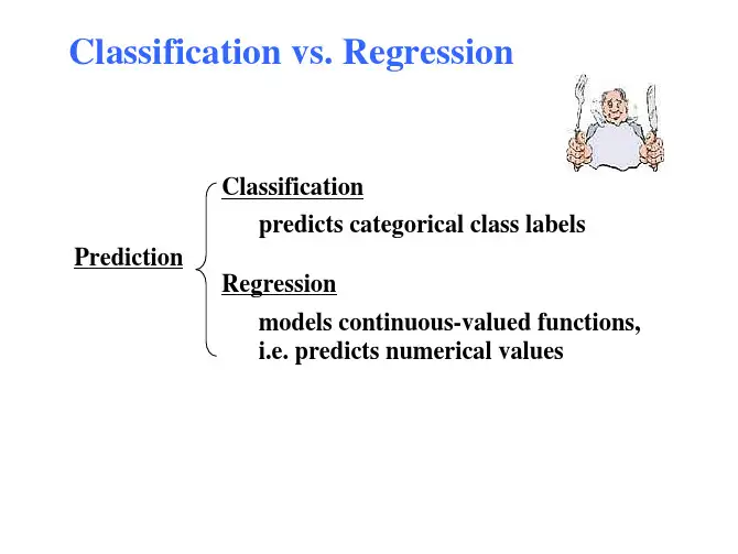
Using Semi-Supervised Clustering to Improve Regression Test Selection Techniques∗
Songyu Chen1,2, Zhenyu Chen1,2,§, Zhihong Zhao1,2, Baowen Xu1, Yang Feng1,2 1 State Key Laboratory for Novel Software Technology, Nanjing University, China
2 Software Institute, Nanjing University, China
§Corresponding author: zychen@software.nju.edu.cn
∗ The work described in this article was partially supported by the National Natural Science Foundation of China (90818027, 60803007,
61003024), the National High Technology Research and Development Program of China (863 Program: 2009AA01Z147), the Major State Basic Research Development Program of China (973 Program: 2009CB320703).
ABSTRACT Cluster test selection is proposed as an efficient regression testing approach. It uses some distance measures and clustering algorithms to group tests into some clusters. Tests in a same cluster are considered to have similar behaviors. A certain sampling strategy for the clustering result is used to build up a small subset of tests, which is expected to approximate the fault detection capability of the original test set. All existing cluster test selection methods employ unsupervised clustering. The previous test results are not used in the process of clustering. It may lead to unsatisfactory clustering results in some cases. In this paper, a semi-supervised clustering method, namely semi-supervised K-means (SSKM), is introduced to improve cluster test selection. SSKM uses limited supervision in the form of pairwise constraints: Must-link and Cannot-link. These pairwise constraints are derived from previous test results to improve clustering results as well as test selection results. The experiment results illustrate the effectiveness of cluster test selection methods with SSKM. Two useful observations are made by analysis. (1) Cluster test selection with SSKM has a better effectiveness when the failed tests are in a medium proportion. (2) A strict definition of pairwise constraint can improve the effectiveness of cluster test selection with SSKM.
Keywords Test selection, regression testing, semi-supervised clustering, pairwise constraint, K-means.
1. INTRODUCTION Regression testing is performed on modified software to provide confidence that the software behaves correctly and modifications have not adversely impacted the software quality by reusing existing tests [21]. Since new faults will be
potentially introduced during the modification of programs, regression testing plays an important role in the lifecycle of software development and maintenance [26,27].
However, regression testing is an expensive process due to the fact that the test set increases during the iterative development process. Running the whole test set is an unacceptable strategy in practice because the testing will exhaust the limited resources. An alternative strategy, test selection, is proposed to choose a small but effective subset of the original test set [13, 19, 28, 29, 34].
In recent years, cluster test selection is proposed as an efficient method in regression testing and observation-based testing [17, 18,
32, 34]. Cluster test selection groups tests into some clusters through establishing some dissimilarity (distance) measures. The distance measures are based on the historical execution profiles of tests. Tests with similar profiles will be grouped into same clusters. It is expected that tests which can detect same faults can be put together. And then, a certain sampling strategy is used to select the representative tests from each cluster [32]. Clustering plays a key role in the process of cluster test selection. A good cluster result can well distinguish passed and failed tests, such that we can construct a small test set which has strong fault detection capability. This inspires us to improve cluster results, as well as test selection results.
In machine learning, clustering is an unsupervised learning of a hidden data concept [7]. This technique uses unlabeled data for training and organizing data into clusters. As an unsupervised data analysis procedure, the clustering results depend on the input parameters, such as the number of clusters or the seeds of data [8]. On the other hand, labeled data is useful for the learning results. Labeled data is often limited and expensive to generate, since the labeled information typically requires human expertise and domain knowledge [6,10,12]. In some applications, labeled information can be extracted from partial results or some evidences in advance, such that both unlabeled data and labeled data are available in the applications. Hence the clustering methods using both unlabeled data and labeled data have attracted many researchers. These methods are so-called semi-supervised clustering [1, 2, 5, 6, 9-12, 14, 16].