计量经济学英文资料Further Quantitative Methods
- 格式:pdf
- 大小:660.33 KB
- 文档页数:10
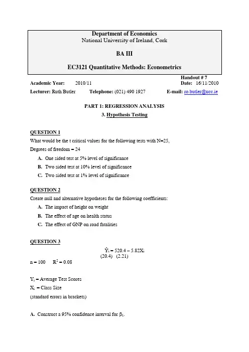
Academic Year:2010/11Date:16/11/2010 Lecturer: Ruth Butler Telephone: (021) 490 1927 E-mail:ro.butler@ucc.iePART 1: REGRESSION ANALYSIS3. Hypothesis TestingQUESTION 1What would be the t critical values for the following tests with N=25,Degrees of freedom = 24A.One sided test at 5% level of significanceB.Two sided test at 10% level of significanceC.Two sided test at 1% level of significanceQUESTION 2Create null and alternative hypotheses for the following coefficients:A.The impact of height on weightB.The effect of age on health statusC.The effect of GNP on road fatalitiesQUESTION 3Ŷi = 520.4 – 5.82X i(20.4) (2.21)n = 100 R2 = 0.08Y i = Average Test ScoresX i = Class Size(standard errors in brackets)A. Construct a 95% confidence interval for 1.B. Test the significance of the slope coefficient at the 5% level of significance. Approximate the p-value for this test.C. Test the null hypothesis that β1 = -5.6 at the 5% level of significance. Compare this answer with your answer for part (A). What can you infer from your comparison?QUESTION 4mt it r r0598.17264.0ˆ+=(0.3001) (0.0728)n = 240 R 2 = 0.471 (standard errors in brackets)r it = the rate of return on the ith security in time t r mt = the rate of return on the market portfolio in time t.A security, whose beta coefficient (ie β1) is greater than one is said to be a volatile or aggressive security. Was IBM a volatile security in the time period under study?QUESTION 5Consider the following hypothetical equation for a sample of divorced men who failed to make at least one child support payment in the last four years (standard errors in parentheses).ii i i i i C B A Y M P 15.00.380.00.2550.00.2ˆ-++++= (0.1) (20) (1) (3) (0.05) Where:Pi = the number of monthly child support payments that the ith man missed in the last four yearsMi = the number of months the ith man was unemployed in the last four yearsYi = the percentage of disposable income that goes to child support payments for the ith man Ai = the age in years of the ith manBi = the religious beliefs of the ith man (a scale of 1 to 4, with 4 being the most religious) Ci = the number of children the ith man has fatheredA.Your friend expects the coefficients of M and Y to be positive. Test these hypotheses.(Use the 5% level at N=20)B.Test the hypotheses that the coefficient of A is different from zero. (Use the 1% levelat N =25)C.Develop the test hypotheses for the coefficients of B and C. ( Use the 10% level andN =17)AnswersQUESTION 1What would be the t critical values for the following tests with N=25 and K= 4?A. One sided test at 5% level of significanceDegrees of Freedom = 21@ 5% α = 0.05 for 1 tailed testt-crit = 1.721Degrees of Freedom = 24@ 5% α = 0.05 for 1-tailed testt-crit = 1.711B.Two sided test at 10% level of significanceDegrees of Freedom = 21@ 10% α = 0.1t crit = 1.721Degrees of Freedom = 24@ 10% α = 0.1t-crit = 1.711C.Two sided test at 1% level of significanceD.F = 21@ 1% α = 0.01t crit = 2.831D.F = 24 @ 1% α = 0.01 t-crit = 2.797QUESTION 2Create null and alternative hypotheses for the following coefficients: A. The impact of height on weight(1-Tailed Test) 0:0:0>≤ββAHHB. The effect of Age on Health Status(1-Tailed Test) 0:0:0<≥ββAHHC. The effect of GNP on Road Fatalities(2-Tailed Test) 0:0:0≠=ββAHHQUESTION 3A. Construct a 95% confidence interval for β1.Confidence Interval = k βˆ± t crit *)βˆse(kCritical value:1) Two sided test for confidence interval2) Level of significance: 95% confidence interval → α = 0.05 3) Degrees of freedom: n – k = 100 – 2 = 98Therefore, t-critical value is 1.984 (approx)95% Confidence Interval = –5.82 ± 1.984*2.21= –5.82 ± 4.38464Therefore the confidence interval is: –10.2046 ≤ β1 ≤ –1.43536This interpreted as meaning the true population coefficient would lie in the above intervals in 95 out of 100 repeated samples.B. Test the significance of the slope coefficient at the 5% level of significance. Approximate the p-value for this test.H 0: 0ˆ1=β H a : 0ˆ1≠β t-statistic = )ˆ(.ˆˆ101βββError Std H - = 21.2082.5-- = -2.63348 = |-2.63348|Critical value: 1) Two tailed test2) Level of significance: 5% → α = 0.053) Degrees of freedom: n - k = 100 – 2 = 98Therefore, the t-critical value is 1.984 (approx)As the t-statistic exceeds the t-critical value, we can reject the null hypothesis at the 5% level of significance and conclude that 1ˆβ is statistically different from zero, therefore the estimate of the slope coefficient is significant.As the estimate for the slope coefficient is significant, the approximate p-value for this test would be a little under 0.01.C. Test the null hypothesis that β1 = -5.6 at the 5% level of significance. Compare this answer with your answer for part (A). What can you infer from your comparison?H 0: 6.5ˆ1-=β H a : 6.5ˆ1-≠βt-statistic = )ˆ(.ˆˆ101βββError Std H -=21.26.582.5+-= -0.09955 = |-0.09955|Critical value: 1) Two tailed test2) Level of significance: 5% → α = 0.053) Degrees of freedom: n - k = 100 – 2 = 98Therefore, the t-critical value is 1.984 (approx)As the t-statistic does NOT exceed the t-critical value, we cannot reject the null hypothesis at the 5% level of significance and thereby conclude that 1ˆβ is not statistically different from –5.6. We would expect this answer since –5.6 lies in the confidence interval calculated in part A.QUESTION 4mt it r r0598.17264.0ˆ+=(0.3001) (0.0728)n = 240 R 2 = 0.471(standard errors in brackets)r it = the rate of return on the ith security in time t r mt = the rate of return on the market portfolio in time t.A security, whose beta coefficient (i.e. β1) is greater than one is said to be a volatile or aggressive security. Was IBM a volatile security in the time period under study? H 0: 1ˆ1≤β H a : 1ˆ1 β t-statistic = )ˆ(.ˆˆ101βββError Std H -=0728.010598.1-= 0.821Critical value: 1) One-tailed test2) Levels of significance: 1%, 5% 10% → α = 0.01, 0.05, 0.13) Degrees of freedom: n - k = 240 – 2 = 238Therefore, the t-critical values are 2.364, 1.660, and 1.290 (approx)As the t-statistic does not exceed the t-critical value we cannot reject the null hypothesis at any of the levels of significance. We can thereby conclude that IBM was not a volatile security over the sample period, as the associated beta was not greater than 1.QUESTION 5Consider the following hypothetical equation for a sample of divorced men who failed to make at least one child support payment in the last four years (standard errors in parentheses)ii i i i i C B A Y M P 15.00.380.00.2550.00.2ˆ-++++= (0.1) (20) (1) (3) (0.05) Where:Pi = the number of monthly child support payments that the ith man missed in the last four yearsMi = the number of months the ith man was unemployed in the last four yearsYi = the percentage of disposable income that goes to child support payments for the ith manAi = the age in years of the ith manBi = the religious beliefs of the ith man (a scale of 1 to 4, with 4 being the most religious) Ci = the number of children the ith man has fatheredA. Your friend expects the coefficients of M and Y to be positive. Test these hypotheses.(Use the 5% level at N=20)0ˆ:0ˆ:10>≤MMH Hββ∴ it is a 1 tailed testDecision Rule: If the t statistic is greater than the critical value, you can reject the null hypothesis.Find t stat:MOE S t HM stat βββˆ.ˆ-==10.050.- = 5Find t crit:@ 5% alpha = 0.05 and d.f = n-k = 20-6 = 14761.1=crit tSince the absolute value of the t statistic does exceed the critical value of t = 1.761 at the 5% level (one-tailed test) and n-k = 20-6 = 14df, we conclude that βm is statistically greater than zero at the 5% level and is significant. (i.e we reject the null hypothesis that βm = 0)0ˆ:0ˆ:1>≤YY H Hββ∴ it is a 1 tailed testDecision Rule: If the t statistic is greater than the critical value, you can reject the null hypothesis.Find t stat:YOE S t HY stat βββˆ.ˆ-==20025- = 1.25Find t crit:@ 5% alpha = 0.05 and d.f = n-k = 20-6 = 14761.1=crit tSince the absolute value of the t statistic does not exceed the critical value of t =1.761 at the 5% level (one-tailed test) and n-k = 20 - 6 = 14 df, we cannot reject the nullhypothesis and conclude that by is not statistically greater than zero at the 5% level and is insignificant.B. Test the hypotheses that the coefficient of A is different from zero. (Use the 1% levelat N =25)0ˆ:0ˆ:10≠=AAH Hββ∴it is a 2 tailed testDecision Rule: If the t statistic is greater than the critical value, you can reject the null hypothesis.Find t stat:AOE S t HA stat βββˆ.ˆ-==108.- = .8Find t crit:@ 1% alpha = 0.01 and d.f = n-k = 25-6 = 19861.2=crit tSince the absolute value of the t statistic does not exceed the critical value of t=2.861 at the 1% level (two-tailed test) and n-k = 25-6 = 19df, we cannot reject the null hypothesis and conclude that bA is not statistically different from zero at the 1% level and is insignificant.C. Develop the test hypotheses for the coefficients of B and C. ( Use the 10% level andN =17)H 0: 0ˆ≥ββ H a : 0ˆ<ββ ∴it is a 1 tailed testDecision Rule: If the t statistic is greater than the critical value, you can reject the null hypothesis.Find t stat:BOE S t HB stat βββˆ.ˆ-==.303- = 1Find t crit:@ 10% alpha = 0.1 and d.f = n - k = 17-6 = 11363.1=crit tSince the absolute value of the t statistic does not exceed the critical value of t=1.363 at the 10% level (one-tailed test) and n-k = 17-6 = 11df, we cannot reject the null hypothesis and conclude that bb is not statistically greater than zero at the 10% level and is insignificant.0ˆ:0ˆ:0 C aC H Hββ≤ ∴ it is a 1 tailed testDecision Rule: If the t statistic is greater than the critical value, you can reject the null hypothesis.Find t stat:C O E S t H C stat βββˆ.ˆ-= = 05.015.-- = -3Find t crit:@ 10% alpha = 0.1 and d.f = n-k = 17-6 = 11363.1=crit tEven though |-3| is greater than the t-critical value of 1.363, we cannot reject the null hypothesis as the t-statistic is not positive as stated in the alternative hypothesis. Therefore, we cannot reject the null hypothesis at the 5% level of significance and conclude that the slope coefficient is not statistically significant.。


伍德里奇计量经济学导论第六版英文课件Woodridge's Introduction to Econometrics, 6th Edition, is a comprehensive textbook that covers the fundamentals of econometrics in a clear and concise manner. The accompanying courseware is designed to help students further understand and apply the concepts discussed in the book.The courseware includes PowerPoint slides, practice quizzes, and interactive exercises to enhance students' learning experience. The slides cover the key topics in each chapter, providing visual aids to help students grasp complex concepts. The quizzes allow students to test their understanding of the material and receive immediate feedback on their performance. The interactive exercises provide hands-on practice withreal-world data sets, helping students develop their econometric skills.In addition to the courseware, students have access to online resources such as supplementary readings, video tutorials, and self-assessment tools. These resources are designed to support students in their learning journey and provide additional assistance when needed.Overall, Woodridge's Introduction to Econometrics, 6th Edition, is a valuable resource for students studying econometrics. The comprehensive courseware offers a range of tools to support students in their learning, making it easier for them to understand and apply the concepts discussed in the textbook. With its clear explanations and practical exercises, this courseware is an essential companion for students looking to excel in econometrics.。

一、计量经济学基本概念二、计量经济学与相关学科的关系三一、计量经济学基本概念二、计量经济学与相关学科的关系三、计量经济学的学科体系四、建立计量经济学模型的步骤和要点五、计量经济学的应用第一章计量经济学概述一、计量经济学基本概念1.计量经济学2.计量经济学的产生 3.计量经济学的定义 4.计量经济学的地位计量经济学是经济学的一个分支学科,是以揭示经济活动中客观存在的数量关系为内容的分支学科。
在有关的出版物和课程表中出现了“计量经济学”与“经济计量学”两种名称。
“经济计量学”是由英文“econometrics”直译得到的,而且强调该学科的主要内容是经济计量的方法,是估计经济模型和检验经济模型;“计量经济学”则试图通过名称强调它是一门经济学科,强调它的经济学内涵与外延。
什么是计量经济学○1926年挪威经济学家R.Frisch提出Econometrics这一学科名称;○ 1930年成立世界计量经济学会;○ 1933年创刊《Econometrica》;○ 20世纪40、50年代的大发展和60年代的扩张;○ 20世纪70年代以来非经典(现代)计量经济学的发展~~~~计量经济学的产生费里希在Econometrica的创刊辞中这样指出:“用数学方法处理经济学可以有多种形式,其中任何单独的一种都不等同于计量经济学,计量经济学不等同于统计学,计量经济学也不等同于我们称之为的一般经济理论(即使这种理论的大部分具有定量的特点),当然,计量经济学也不是数学在经济学中的应用的同义词。
不用说,统计学、经济理论和数学是理解现代经济生活中的数量关系所不可缺少的必要条件,但是作为充分条件的是这三者的结合,这三者的结合就构成了计量经济学。
”定义计量经济学的地位计量经济学是一门经济学科。
首先,从定义看,计量经济学是统计学、经济理论和数学三者的结合,这种结合说明它是定量化的经济学或者经济学的定量化;其次,从经济学科中的地位看,计量经济学已经在在西方国家的经济学科中占有重要地位,在大多数大学和学院中,计量经济学的讲授已经成为经济学课程表中最有权威的部分。

伍德里奇计量经济学导论第6版考研笔记和课后习题详解伍德里奇《计量经济学导论》(第6版)笔记和课后习题详解内容简介伍德里奇所著的《计量经济学导论》(第6版)是我国许多高校采用的计量经济学优秀教材,也被部分高校指定为“经济类”专业考研考博参考书目。
本书遵循伍德里奇《计量经济学导论》(第6版)教材的章目编排,共分3篇19章,每章由两部分组成:第一部分为复习笔记,总结本章的重难点内容;第二部分为课(章)后习题详解,对第6版的所有课(章)后习题都进行了详细的分析和解答。
作为该教材的学习辅导书,本书具有以下几个方面的特点:(1)整理名校笔记,浓缩内容精华。
每章的复习笔记以伍德里奇所著的《计量经济学导论》(第6版)为主,并结合国内外其他计量经济学经典教材对各章的重难点进行了整理,因此,本书的内容几乎浓缩了经典教材的知识精华。
(2)解析课后习题,提供详尽答案。
本书参考大量经济学相关资料对伍德里奇所著的《计量经济学导论》(第6版)的课(章)后习题进行了详细的分析和解答,并对相关重要知识点进行了延伸和归纳。
(3)补充相关要点,强化专业知识。
一般来说,国外英文教材的中译本不太符合中国学生的思维习惯,有些语言的表述不清或条理性不强而给学习带来了不便,因此,对每章复习笔记的一些重要知识点和一些习题的解答,我们在不违背原书原意的基础上结合其他相关经典教材进行了必要的整理和分析。
•试看部分内容第1章计量经济学的性质与经济数据1.1复习笔记考点一:计量经济学及其应用★1计量经济学计量经济学是在一定的经济理论基础之上,采用数学与统计学的工具,通过建立计量经济模型对经济变量之间的关系进行定量分析的学科。
进行计量分析的步骤主要有:①利用经济数据对模型中的未知参数进行估计;②对模型进行检验;③通过检验后,可以利用计量模型来进行相关预测。
2经济分析的步骤经济分析是指利用所搜集的相关数据检验某个理论是否成立或估计某种关系的方法。
经济分析主要包括以下几步,分别是阐述问题、构建经济模型、经济模型转化为计量模型、搜集相关数据、参数估计和假设检验。

计量经济学常用英语词汇,都在这里了!计量经济学常用英语词汇集锦Absolute deviation, 绝对离差Absolute residuals, 绝对残差Acceleration in an arbitrary direction, 任意方向上的加速度Acceleration normal, 法向加速度Acceleration space dimension, 加速度空间的维数Acceleration tangential, 切向加速度Acceleration vector, 加速度向量Acceptable hypothesis, 可接受假设Actual frequency, 实际频数Adaptive estimator, 自适应估计量Addition theorem, 加法定理Additive Noise, 加性噪声Adjusted rate, 调整率Adjusted value, 校正值Admissible error, 容许误差Alpha factoring,α因子法Alternative hypothesis, 备择假设Analysis of correlation, 相关分析Analysis of covariance, 协方差分析Analysis Of Effects, 效应分析Analysis Of Variance, 方差分析Analysis of regression, 回归分析Analysis of time series, 时间序列分析Angular transformation, 角转换ANOVA Models, 方差分析模型Arcsine transformation, 反正弦变换Area under the curve, 曲线面积AREG , 评估从一个时间点到下一个时间点回归相关时的误差ARIMA, 季节和非季节性单变量模型的极大似然估计Arithmetic grid paper, 算术格纸Arrhenius relation, 艾恩尼斯关系Asymptotic efficiency, 渐近效率Asymptotic variance, 渐近方差Attributable risk, 归因危险度Autocorrelation of residuals, 残差的自相关Bar chart, 条形图Bar graph, 条形图Base period, 基期Bayes' theorem , Bayes定理Bell-shaped curve, 钟形曲线Bernoulli distribution, 伯努力分布Best-trim estimator, 最好切尾估计量Binary logistic regression, 二元逻辑斯蒂回归Binomial distribution, 二项分布Bisquare, 双平方Bivariate Correlate, 二变量相关Bivariate normal distribution, 双变量正态分布Bivariate normal population, 双变量正态总体Biweight interval, 双权区间Biweight M-estimator, 双权M估计量Block, 区组/配伍组BMDP(Biomedical computer programs), BMDP统计软件包Boxplots, 箱线图/箱尾图Breakdown bound, 崩溃界/崩溃点Canonical correlation, 典型相关Case-control study, 病例对照研究Categorical variable, 分类变量Cauchy distribution, 柯西分布Center of symmetry, 对称中心Centering and scaling, 中心化和定标Central tendency, 集中趋势Central value, 中心值CHAID -χ2 Auto matic Interaction Detector, 卡方自动交互检测Chance error, 随机误差Chance variable, 随机变量Characteristic equation, 特征方程Characteristic root, 特征根Characteristic vector, 特征向量Chebshev criterion of fit, 拟合的切比雪夫准则Chernoff faces, 切尔诺夫脸谱图D test, D检验Data acquisition, 资料收集Data bank, 数据库Data capacity, 数据容量Data deficiencies, 数据缺乏Data handling, 数据处理Data manipulation, 数据处理Data processing, 数据处理Data reduction, 数据缩减Data sources, 数据来源Data transformation, 数据变换Data validity, 数据有效性Dead time, 停滞期Degree of freedom, 自由度Degree of precision, 精密度Degree of reliability, 可靠性程度Degression, 递减Density function, 密度函数Error Bar, 均值相关区间图Effect, 实验效应Eigenvalue, 特征值Eigenvector, 特征向量Empirical distribution, 经验分布Empirical probability, 经验概率单位Enumeration data, 计数资料Equal sun-class number, 相等次级组含量Equally likely, 等可能Equivariance, 同变性Error, 误差/错误Error of estimate, 估计误差Error type I, 第一类错误Error type II, 第二类错误Estimand, 被估量Estimated error mean squares, 估计误差均方Estimated error sum of squares, 估计误差平方和Euclidean distance, 欧式距离Exceptional data point, 异常数据点Expectation plane, 期望平面Expectation surface, 期望曲面Expected values, 期望值Experiment, 实验F distribution, F分布F test, F检验Factor, 因素/因子Factor analysis, 因子分析Factor score, 因子得分Factorial design, 析因试验设计False negative, 假阴性False negative error, 假阴性错误Family of distributions, 分布族Family of estimators, 估计量族Fatality rate, 病死率Gamma distribution, 伽玛分布Gauss increment, 高斯增量Gaussian distribution, 高斯分布/正态分布Gauss-Newton increment, 高斯-牛顿增量General census, 全面普查Generalized least squares, 综合最小平方法GENLOG (Generalized liner models), 广义线性模型Geometric mean, 几何平均数Gini's mean difference, 基尼均差GLM (General liner models), 通用线性模型Goodness of fit, 拟和优度/配合度Gradient of determinant, 行列式的梯度Graeco-Latin square, 希腊拉丁方Grand mean, 总均值Gross errors, 重大错误。
计量经济学参考书目计量经济学入门:Griffiths, W. E., R. C. Hill, and G. G. Judge, 1993, Learning and Practicing Econometrics, John Wiley & Sons. Johnston, J. and J. DiNardo, 1997, Econometric Methods, 4th ed., McGraw-Hill.Maddala, G. S., 1992, Introduction to Econometrics, 2nd ed., Prentice-Hall. Ramanathan, R., 1998, Introductory Econometrics with Applications, 4th ed., The Dryden Press.(前四本似乎是大学程度计量经济学教科书中最为流行者)Judge, G. G., W. E. Griffiths, R. C. Hill, T.-C. Lee, and H. Lutkepol, 1988, Introduction to the Theory and Practice of Econometrics, 2nd ed.,John Wiley & Sons. Kennedy, P., 1998, A Guide to Econometrics, 4th. ed. The MIP Press. (本书尝试少用数学而多以文字来解释一些计量经济学的概念)Goldberger, A. S., 1991, A Course in Econometrics, Harvard University Press. (本书善用简单例子解释一些重要的基本观念,本书缺点在于未能包括一些新课题)Gujarati, D. N., 1995, Basic Econometrics, 3nd. ed., McGraw-Hill. Thomas, R. L., 1996, Modern Econometrics, An Introduction, Addison-Wesley. Lardaro, L., 1993, Applied Econometrics, Harper Collins.(书中包含了一些实例应用)Ghosh, S. K., 1991, Econometrics: Theory and Applications, Prentice-Hall.(书中包含了一些实例应用)Hill, R. C., W. E. Griffiths, and G. G. Judge, 1997, Undergraduate Econometrics, Jogn Wiley & Sons. (本书较薄较浅,适合统计学基础较弱的读者)Draper, N. R. and H. Smith, 1998, Applied Regression Analysis, John Wiley & Sons. (本书和下一本书均是非计量经济学者学回归分析常用的教科书)Neter, J. and W. Wasserman, 1996, Applied Linear Statistical Models, 4th ed., Irwin.中级计量经济学:Greene, W. H., 1997, Econometric Analysis, 3rd ed., Prentice-Hall , Inc.(最畅销的研究所计量经济学教科书,包含范围很广,但常有解释不清的地方。
FQRM ZHOU RUOQIAN 1 / 10 MULTIPLE REGRESSION MODEL Multicollinearity OLS assumption 8. No exact collinearity between the X variables. If two or more variables are perfectly collinear, det(X’X) = 0 and (X’X) cannot be inverted and we cannot estimate the parameters of interest by OLS. If det(X’X) is close to zero, we have (near) multicollinearity. OLS estimators are still BLUE. Consequences of near multicollinearity: 1. OLS estimators are still BLUE. 无偏,方差最小 2. The OLS estimators have large variances and covariance, making precise estimation difficult. 方差最小但是很大,误差大难以估计参数精确值 3. The confidence intervals tend to be much wider, leading to the acceptance of the “zero null hypothesis”. 误差大,置信区间变宽,容易接受H0 4. The t ratio of one or more coefficients tends to be statistically insignificant. t值会很小,不显著 5. Although the t ratio of one or more coefficients is statistically insignificant, 𝑅2, the overall measure of goodness of fit, can be very high. 不过R2还是显示很大 6. The OLS estimators and their standard errors can be sensitive to small changes in the data. OLS估计量和标准误差对数据变动很敏感,即不稳定 Detection:度量多重共线性的程度,而不是存在与否 -1) High 𝑅2 but few significant t ratios.典型特征 -2) High pair-wise correlations among regressors.解释变量相关系数高,这个标准不一定可靠 -3) Examination of partial correlations.检验偏相关系数,也不可靠 -4) Auxiliary regressions:辅助回归 -5) Scatterplot VIF test -𝑅𝑗2=𝑅2 in the regression of 𝑋𝑗 on the remaining 𝑘−2 regressors. 是𝑋𝑗 对剩余变量辅助回归的样本判定系数The
variance 𝑉(𝛽𝑗) gets higher the larger 𝑅𝑗2 gets. The first term of the formula is the variance inflation factor (VIF), 𝑉𝐼𝐹𝑗=1/1−𝑅𝑗2. The inverse of VIF, 1− 𝑅𝑗
2
, is called tolerance.
-If 𝑋𝑗 is highly correlated with the other X variables, then 𝑅𝑗2
will be large, hence the VIF will be large as well.
-A large VIF inflates the variance of 𝛽𝑗, making it difficult to obtain a significant t-ratio.
-Thus if multicollinearity exists, probably the standard errors of the parameter estimates will all be inflated. -Typically, the value of 10 is used as a threshold at which we consider it to be a problem, but this is simply a rule of thumb. Remedial measures: Do nothing or the following没有万无一失的好方法 FQRM ZHOU RUOQIAN 2 / 10 -1) A prior information, used to reduce collinearity.先验信息。直接知道其中一个参数的值 -2) Combining cross-sectional and time series data结合两种数据 -3) Dropping a variable(s) and specification bias.删变量和设定误差,可能导致模型不对 -4) Transformation of variables.变量转换。如:名义转化为实际 -5) Additional or new data新数据。多重共线性是样本特征,多一点样本数据可能有用 -6) Reducing collinearity in polynomial regressions: expressing explanatory variables in deviation form, orthogonal polynomials.减少多项式回归里的共线性,用离差形式展示解释变量,正交多项式 -7) Other methods of remedying multicollinearity: factor analysis, principal components, ridge regression.因子分析,主成分回归,岭回归 FQRM ZHOU RUOQIAN
3 / 10 Heteroscedasticity
多存在横截面数据而不是时间序列数据,可能是样本规模不同,引起规模效应(scale effects) CLRM Assumption 4. 𝑬𝒖𝒊=𝝈𝟐, 𝒊=𝟏,𝟐,⋯,𝒏. Heteroscedasticity: the disturbances do not have constant, identical variances. When Var (u|X) depends on X, we say that the error term is heteroskedastic. 𝐸𝑢𝑖=𝜎𝑖2, 1,2,⋯,𝑛. Consequences: Heteroskedasticity does not cause bias or inconsistency in the OLS estimators of the 𝛽s. -1) Var (bj) is biased. Since the OLS standard errors are used to compute the t statistics and related intervals, the usual OLS t statistics have no longer t distribution and become invalid (overestimated). -2) All the other statistics (F for instance) used to test hypotheses are no longer valid (overestimated). -3) If Var (u|X) is not constant, OLS estimators are not BLUE. -估计值无偏稳定,但方差不是最小。残值方差有偏,导致估计量方差有偏,t和F以及置信区间假设检验都无效了。 Detection: -1) Graphic method, scatter diagram of squared residuals against fitted values of Y. If there is a systematic trend, there is heteroscedasticity problem.看ei2和Y的散点图,看有无特定趋势 -2) Formal methods: Park test Glejser test Spearman’s Rank correlation test Goldfeld-Quandt test Breusch-Pagan-Godfrey test, White’s General Heteroscedasticity test Remedy -The first approach to deal with heteroscedasticity is to use Weighted Least Squares (WLS) regression instead of Ordinary Least Squares regression. -The second and increasingly popular way of dealing with heteroskedasticity is to run OLS regression but compute the variance of the estimates using the formula which takes into account of heteroskedasticity. 校正误差方差 STATA have this formula built in as heteroskedasticity-robust regression