FLUENT-MDM-tut-06_vane-pump

本教程以泵内定常流动数值模拟为例，详细讲述了如何应用FLUENT进行泵内流计算以及如何应用FLUENT进行简单的后处理。

基本步骤：1、启动FLUENT，选择3d求解器。

2、读入网格（×.msh）；3、检查网格，确保最小体积为正，选择grid→check菜单；4、缩放网格；5、光顺/交换网格；6、求解器设置；7、设置计算模型；8、设置运行环境，对于离心泵数值模拟一般不考虑重力；9、设置转速单位；10、定义材料，也可以进行自定义材料；11、定义边界条件；12、设置交界面；13、设置求解参数；14、监视残差；15、初始化流场；16、保存case文件；17、开始迭代计算；18、FLUENT后处理。

1、启动FLUENT，选择3d求解器。

启动后FLUENT界面如下图所示：2、读入网格（×.msh），选择file→read→case菜单；3、检查网格，确保最小体积为正，选择grid→check菜单。

Check无误后才可以进行下面的操作。

4、缩放网格，选择grid→scale菜单，弹出下图的对话框，直接输入Scale Factors点击Scale即可，一般缩小1000倍到毫米。

由于FLUENT默认的单位是米，所以必须进行网格缩放。

5、光顺/交换网格，选择grid→smooth/swap菜单，进入下面的界面；先点击Smooth，然后点击Swap直至Number Swapped为0。

6、求解器设置，选择define→models→solver菜单，进入求解器设置界面，如下图所示。

一般定常求解设置为分离求解器、隐式算法、三维空间、稳态流动、绝对速度、压力梯度为单元压力梯度计算；7、设置计算模型，选择define→models→viscous菜单，弹出湍流模型选择对话框。

一般选用标准k-ε模型，进入k-ε模型设置界面，一般保持默认即可；8、设置运行环境，选择define→operating condition菜单，弹出下面的对话框。

F L U E N T喷雾模拟具体
步骤
公司内部编号：（GOOD-TMMT-MMUT-UUPTY-UUYY-DTTI-
dispersionangle参数很重要
设置的是6?太小了
选择离散相模型DPM（拉格朗日离散粒子多相流）
Discrete Phase Model面板中的Unsteady Parameters 属性框中激活了Unsteady Tracking 选项，在瞬态流动中考虑相间耦合计算，在每一个迭代时间步长内，依据在Number Of Continuous PhaseIterations Per DPM Iteration 设定的迭代步数进行颗粒轨道的迭代计算。

液滴破碎模型：泰勒类比破碎模型
FLUENT 提供两种雾滴破碎模型：泰勒类比破碎（TAB）模型和波致破碎模型。

本文选自泰勒类比破碎模型。

Discrete Phase Model-Spray Models 下激活Droplet Breakup，TAB 模型，设置y0为0.001（初始变形值）
动态曳力模型
创建入射源：
创建喷雾模型：选择pressure-swirl-atomizer（压力旋流雾化模型）水滴颗粒相流数目：
水滴颗粒相设置：
惯性颗粒（``inert''）离散相类型（颗粒、液滴或气泡）
材料设置：
属性设置：
入射源位置
入射源轴向方向设置：
流量以及时间设置：喷嘴直径，锥角，重力加速度设置：。

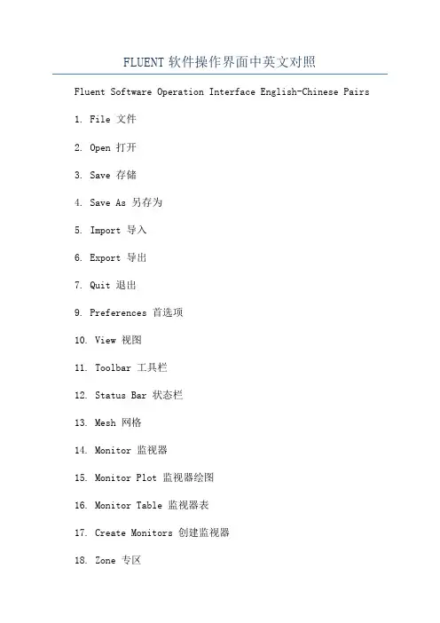
FLUENT软件操作界面中英文对照Fluent Software Operation Interface English-Chinese Pairs1. File 文件2. Open 打开3. Save 存储4. Save As 另存为5. Import 导入6. Export 导出7. Quit 退出9. Preferences 首选项10. View 视图11. Toolbar 工具栏12. Status Bar 状态栏13. Mesh 网格14. Monitor 监视器15. Monitor Plot 监视器绘图16. Monitor Table 监视器表17. Create Monitors 创建监视器18. Zone 专区19. Operation 操作20. Domain 领域21. Manage 管理22. Tables 表23. Solve 解24. Solve Setup 解决设置26. Boundary Conditions 边界条件27. Definitions 定义28. Solution Monitors 解决监视器29. Global Parameters 全局参数30. Flow Models 流动模型31. Turbulence Models 湍流模型32. Species Models 种类模型33. Initialization 初始化34. Time-Scale & Pressure Control 时间尺度压力控制35. Advanced ODE Solver 高级常微分方程求解36. Solution Controls 解决控制37. Residual Controls 残余控制38. Memory & Multigrid Controls 内存&多重网格控制39. Under Relaxation 松弛40. Discrete Transfer 离散传递41. Refine Mesh 细化网格42. Reporting 报告43. Monitors 监视器44. Post Processing 后处理45. Mode 状态46. Graph 语句47. Residuals 残余48. Contours等值线49. Vectors 矢量50. Point Monitors 点监视器51. Interrogate 查询52. Probe Measurements 探针测量53. Construct Geometry 构造几何体54. Geometry 构造55. Extrude 拉伸56. Merge 合并57. Make Map 构建图58. Close Gaps 关闭间隙59. Round Corners 圆角60. Rotate 旋转61. Translate 平移62. Rename 重命名63. Measurements 测量66. Simulation 模拟67. Grid 位格68. Solution 解决69. File Signatures 文件标识70. Tools 工具71. Results 结果72. Data Sets 数据集。

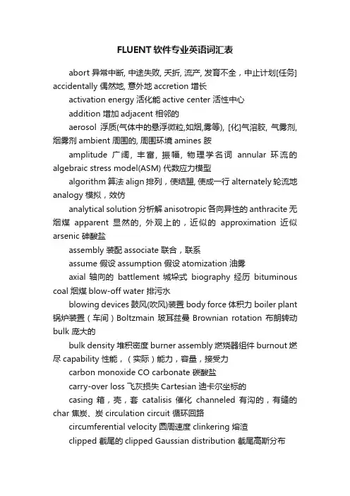
FLUENT软件专业英语词汇表abort 异常中断, 中途失败, 夭折, 流产, 发育不全，中止计划[任务] accidentally 偶然地, 意外地accretion 增长activation energy 活化能active center 活性中心addition 增加adjacent 相邻的aerosol浮质(气体中的悬浮微粒,如烟,雾等), [化]气溶胶, 气雾剂, 烟雾剂ambient 周围的, 周围环境amines 胺amplitude 广阔, 丰富, 振幅, 物理学名词annular 环流的algebraic stress model(ASM) 代数应力模型algorithm 算法align 排列，使结盟, 使成一行alternately 轮流地analogy 模拟，效仿analytical solution 分析解anisotropic 各向异性的anthracite 无烟煤apparent 显然的, 外观上的，近似的approximation 近似arsenic 砷酸盐assembly 装配associate 联合，联系assume 假设assumption 假设atomization 油雾axial 轴向的battlement 城垛式biography 经历bituminous coal 烟煤blow-off water 排污水blowing devices 鼓风(吹风)装置body force 体积力boiler plant 锅炉装置（车间）Boltzmain 玻耳兹曼Brownian rotation 布朗转动bulk 庞大的bulk density 堆积密度burner assembly 燃烧器组件burnout 燃尽capability 性能，（实际）能力，容量，接受力carbon monoxide CO carbonate 碳酸盐carry-over loss 飞灰损失Cartesian 迪卡尔坐标的casing 箱，壳，套catalisis 催化channeled 有沟的，有缝的char 焦炭、炭circulation circuit 循环回路circumferential velocity 圆周速度clinkering 熔渣clipped 截尾的clipped Gaussian distribution 截尾高斯分布closure (模型的)封闭cloud of particles 颗粒云cluster 颗粒团coal off-gas 煤的挥发气体coarse 粗糙的coarse grid 疏网格，粗网格coaxial 同轴的coefficient of restitution 回弹系数；恢复系数coke 碳collision 碰撞competence 能力competing process 同时发生影响的competing-reactions submodel 平行反应子模型component 部分分量composition 成分cone shape 圆锥体形状configuration 布置，构造confined flames 有界燃烧confirmation 证实, 确认, 批准conservation 守恒不灭conservation equation 守恒方程conserved scalars 守恒量considerably 相当地consume 消耗contact angle 接触角contamination 污染contingency 偶然, 可能性, 意外事故, 可能发生的附带事件continuum 连续体converged 收敛的conveyer 输运机convolve 卷cooling wall 水冷壁correlation 关联(式) correlation function 相关函数corrosion 腐蚀，锈coupling 联结, 接合, 耦合crack 裂缝，裂纹creep up （水）渗上来，蠕升critical 临界critically 精密地cross-correlation 互关联cumulative 累积的curtain wall 护墙，幕墙curve 曲线custom 习惯, 风俗, <动词单用>海关, (封建制度下)定期服劳役, 缴纳租税, 自定义, <偶用作>关税v.定制, 承接定做活的cyano 氰（基），深蓝，青色cyclone 旋风子，旋风，旋风筒cyclone separator 旋风分离器[除尘器] cylindrical 柱坐标的cylindrical coordinate 柱坐标dead zones 死区decompose 分解decouple 解藕的defy 使成为不可能demography 统计deposition 沉积derivative with respect to 对…的导数derivation 引出, 来历, 出处, (语言)语源, 词源design cycle 设计流程desposit 积灰，结垢deterministic approach 确定轨道模型deterministic 宿命的deviation 偏差devoid 缺乏devolatilization 析出挥发分，液化作用diffusion 扩散diffusivity 扩散系数digonal 二角(的), 对角的，二维的dilute 稀的diminish 减少direct numerical simulation 直接模拟discharge 释放discrete 离散的discrete phase 分散相, 不连续相discretization [数]离散化deselect 取消选定dispersion 弥散dissector 扩流锥dissociate thermally 热分解dissociation 分裂dissipation 消散, 分散, 挥霍, 浪费, 消遣, 放荡, 狂饮distribution of air 布风divide 除以dot line 虚线drag coefficient 牵引系数，阻力系数drag and drop 拖放drag force 曳力drift velocity 漂移速度driving force 驱[传, 主]动力droplet 液滴drum 锅筒dry-bottom-furnace 固态排渣炉dry-bottom 冷灰斗，固态排渣duct 管dump 渣坑dust-air mixture 一次风EBU---Eddy break up 漩涡破碎模型eddy 涡旋effluent 废气，流出物elastic 弹性的electro-staic precipitators 静电除尘器emanate 散发, 发出, 发源，[罕]发散, 放射embrasure 喷口，枪眼emissivity [物]发射率empirical 经验的endothermic reaction 吸热反应enhance 增，涨enlarge 扩大ensemble 组，群，全体enthalpy 焓entity 实体entrain 携带，夹带entrained-bed 携带床equilibrate 保持平衡equilibrium 化学平衡ESCIMO-----Engulfment（卷吞）Stretching（拉伸）Coherence（粘附）Interdiffusion-interaction（相互扩散和化学反应）Moving-observer（运动观察者）exhaust 用尽, 耗尽, 抽完, 使精疲力尽排气排气装置用不完的, 不会枯竭的exit 出口，排气管exothermic reaction 放热反应expenditure 支出，经费expertise 经验explicitly 明白地, 明确地extinction 熄灭的extract 抽出，提取evaluation 评价，估计，赋值evaporation 蒸发(作用) Eulerian approach 欧拉法facilitate 推动，促进factor 把…分解fast chemistry 快速化学反应fate 天数, 命运, 运气，注定, 送命，最终结果feasible 可行的，可能的feed pump 给水泵feedstock 填料fine grid 密网格，细网格finite difference approximation 有限差分法flamelet 小火焰单元flame stability 火焰稳定性flow pattern 流型fluctuating velocity 脉动速度fluctuation 脉动，波动flue 烟道（气）flue duck 烟道fluoride 氟化物fold 夹层块forced-and-induced draft fan 鼓引风机forestall 防止fouling 沾污fraction 碎片部分，百分比fragmentation 破碎fuel-rich regions 富燃料区，浓燃料区fuse 熔化，熔融gas duct 烟道gas-tight 烟气密封gasification 气化(作用)gasifier 气化器generalized model 通用模型Gibbs function Method 吉布斯函数法Gordon 戈登governing equation 控制方程gradient 梯度graphics 图gross efficiency 总效率hazard 危险header 联箱helically 螺旋形地heterogeneous 异相的heat flux 热流(密度)heat regeneration 再热器heat retention coeff 保热系数histogram 柱状图homogeneous 同相的、均相的hopper 漏斗horizontally 卧式的，水平的hydrodynamic drag 流体动力阻力hydrostatic pressure 静压hypothesis 假设humidity 湿气，湿度，水分含量identical 同一的，完全相同的ignition 着火illustrate 图解，插图in common with 和…一样in excess of 超过, 较...为多in recognition of 承认…而，按照in terms of 根据, 按照, 用...的话, 在...方面incandescent 白炽的，光亮的inception 起初induced-draft fan 强制引风机inert 无活动的, 惰性的, 迟钝的inert atmosphere 惰性气氛inertia 惯性, 惯量inflammability 可燃性injection 引入，吸引inleakage 漏风量inlet 入口inlet vent 入烟口instantaneous reaction rate 瞬时反应速率instantaneous velocity 瞬时速度instruction 指示, 用法说明(书), 教育, 指导, 指令intake fan 进气风扇integral time 积分时间integration 积分interface 接触面intermediate 中间的，介质intermediate species 中间组分intermittency model of turbulence 湍流间歇模型intermixing 混合intersect 横断，相交interval 间隔intrinsic 内在的inverse proportion 反比irreverse 不可逆的irreversible 不可逆的，单向的isothermal 等温的, 等温线的,等温线isotropic 各向同性的joint 连接justify 认为Kelvin 绝对温度，开氏温度kinematic viscosity 动粘滞率, 动粘度kinetics 动力学Lagrangian approach 拉格朗日法laminarization 层流化的Laminar 层流Laminar Flamelet Concept 层流小火焰概念large-eddy simulation (LES) 大涡模拟leak 泄漏length scale 湍流长度尺度liberate 释放lifetime 持续时间，（使用）寿命，使用期literature 文学(作品), 文艺, 著作, 文献lining 炉衬localized 狭小的logarithm [数] 对数Low Reynolds Number Modeling Method 低雷诺数模型macropore 大孔隙(直径大于1000埃的孔隙)manipulation 处理, 操作, 操纵, 被操纵mass action 质量作用mass flowrate 质量流率Mcbride 麦克布利德mean free paths 平均自由行程mean velocity 平均速度meaningful 意味深长的，有意义的medium 均匀介质mercury porosimetery 水银测孔计, 水银孔率计mill 磨碎，碾碎mineral matter 矿物质mixture fraction 混合分数modal 众数的，形式的, 样式的, 形态上的, 情态的, 语气的[计](对话框等)模式的modulus 系数, 模数moisture 水分，潮湿度molar 质量的, [化][物]摩尔的moment 力矩，矩，动差momentum 动量momentum transfer 动量传递monobloc 单元机组monobloc units 单组mortar 泥灰浆mount 安装，衬底Monte Carlo methods 蒙特卡罗法multiflux radiation model 多(4/6)通量模型multivariate [统][数]多变量的,多元的negative 负Newton-Rephson 牛顿—雷夫森nitric oxide NO2node 节点non-linear 非线性的numerical control 数字控制numerical simulation 数值模拟table look-up scheme 查表法tabulate 列表tangential 切向的tangentially 切线tilting 摆动the heat power of furnace 热负荷the state-of-the-art 现状thermal effect 反应热thermodynamic 热力学thermophoresis 热迁移，热泳threshold 开始, 开端, 极限tortuosity 扭转, 曲折, 弯曲toxic 有毒的，毒的trajectory 轨迹,弹道tracer 追踪者, 描图者, (铁笔等)绘图工具translatory 平移的transport coefficients 输运系数transverse 横向，横线triatomic 三原子的turbulence intensity 湍流强度turbulent 湍流turbulent burner 旋流燃烧器turbulization 涡流turnaround 完成two-scroll burner 双涡流燃烧器unimodal [统](频率曲线或分布)单峰的,(现象或性质) 用单峰分布描述的validate 使…证实validation 验证vaporization 汽化Variable 变量variance 方差variant 不同的，变量variation 变更, 变化, 变异, 变种, [音]变奏, 变调vertical 垂直的virtual mass 虚质量viscosity 粘度visualization 可视化volatile 易挥发性的volume fraction 体积分数, 体积分率, 容积率volume heat 容积热vortex burner 旋流式燃烧器vorticity 旋量wall-function method 壁面函数法water equivalent 水当量weighting factor 权重因数unity （数学）一uniform 不均匀unrealistic 不切实际的, 不现实的Zeldovich 氮的氧化成一氧化氮的过程zero mean 零平均值zone method 区域法。

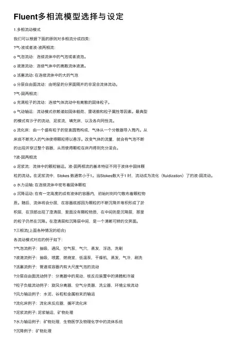
Fluent多相流模型选择与设定1.多相流动模式我们可以根据下⾯的原则对多相流分成四类：⽓-液或者液-液两相流：o ⽓泡流动：连续流体中的⽓泡或者液泡。

o 液滴流动：连续⽓体中的离散流体液滴。

o 活塞流动: 在连续流体中的⼤的⽓泡o 分层⾃由⾯流动：由明显的分界⾯隔开的⾮混合流体流动。

⽓-固两相流：o 充满粒⼦的流动：连续⽓体流动中有离散的固体粒⼦。

o ⽓动输运：流动模式依赖诸如固体载荷、雷诺数和粒⼦属性等因素。

最典型的模式有沙⼦的流动，泥浆流，填充床，以及各向同性流。

o 流化床：由⼀个盛有粒⼦的竖直圆筒构成，⽓体从⼀个分散器导⼊筒内。

从床底不断充⼊的⽓体使得颗粒得以悬浮。

改变⽓体的流量，就会有⽓泡不断的出现并穿过整个容器，从⽽使得颗粒在床内得到充分混合。

液-固两相流o 泥浆流：流体中的颗粒输运。

液-固两相流的基本特征不同于液体中固体颗粒的流动。

在泥浆流中，Stokes 数通常⼩于1。

当Stokes数⼤于1 时，流动成为流化（fluidization）了的液-固流动。

o ⽔⼒运输: 在连续流体中密布着固体颗粒o 沉降运动: 在有⼀定⾼度的成有液体的容器内，初始时刻均匀散布着颗粒物质。

随后，流体将会分层，在容器底部因为颗粒的不断沉降并堆积形成了淤积层，在顶部出现了澄清层，⾥⾯没有颗粒物质，在中间则是沉降层，那⾥的粒⼦仍然在沉降。

在澄清层和沉降层中间，是⼀个清晰可辨的交界⾯。

三相流(上⾯各种情况的组合)各流动模式对应的例⼦如下：⽓泡流例⼦：抽吸，通风，空⽓泵，⽓⽳，蒸发，浮选，洗刷液滴流例⼦：抽吸，喷雾，燃烧室，低温泵，⼲燥机，蒸发，⽓冷，刷洗活塞流例⼦：管道或容器内有⼤尺度⽓泡的流动分层⾃由⾯流动例⼦：分离器中的晃动，核反应装置中的沸腾和冷凝粒⼦负载流动例⼦：旋风分离器，空⽓分类器，洗尘器，环境尘埃流动风⼒输运例⼦：⽔泥、⾕粒和⾦属粉末的输运流化床例⼦：流化床反应器，循环流化床泥浆流例⼦: 泥浆输运，矿物处理⽔⼒输运例⼦：矿物处理，⽣物医学及物理化学中的流体系统沉降例⼦：矿物处理2. 多相流模型FLUENT中描述两相流的两种⽅法:欧拉⼀欧拉法和欧拉⼀拉格朗⽇法，后⾯分别简称欧拉法和拉格朗⽇法。

fluent中一些问题fluent中一些问题----(目录)2010-02-23 13:11:48| 分类：Fluent |举报|字号订阅目录1 如何入门2 CFD计算中涉及到的流体及流动的基本概念和术语2.1 理想流体（Ideal Fluid）和粘性流体（Viscous Fluid）2.2 牛顿流体（Newtonian Fluid）和非牛顿流体（non-Newtonian Fluid）2.3 可压缩流体（Compressible Fluid）和不可压缩流体（Incompressible Fluid）2.4 层流（Laminar Flow）和湍流（Turbulent Flow）2.5 定常流动（Steady Flow）和非定常流动（Unsteady Flow）2.6 亚音速流动(Subsonic)与超音速流动（Supersonic）2.7 热传导（Heat Transfer）及扩散（Diffusion）3 在数值模拟过程中，离散化的目的是什么？如何对计算区域进行离散化？离散化时通常使用哪些网格？如何对控制方程进行离散？离散化常用的方法有哪些？它们有什么不同？3.1 离散化的目的3.2 计算区域的离散及通常使用的网格3.3 控制方程的离散及其方法3.4 各种离散化方法的区别4 常见离散格式的性能的对比（稳定性、精度和经济性）5 流场数值计算的目的是什么？主要方法有哪些？其基本思路是什么？各自的适用范围是什么？6 可压缩流动和不可压缩流动，在数值解法上各有何特点？为何不可压缩流动在求解时反而比可压缩流动有更多的困难？6.1 可压缩Euler及Navier-Stokes方程数值解6.2 不可压缩Navier-Stokes方程求解7 什么叫边界条件？有何物理意义？它与初始条件有什么关系？8 在数值计算中，偏微分方程的双曲型方程、椭圆型方程、抛物型方程有什么区别？9 在网格生成技术中，什么叫贴体坐标系？什么叫网格独立解？10 在GAMBIT中显示的“check”主要通过哪几种来判断其网格的质量？及其在做网格时大致注意到哪些细节？11 在两个面的交界线上如果出现网格间距不同的情况时，即两块网格不连续时，怎么样克服这种情况呢？12 在设置GAMBIT边界层类型时需要注意的几个问题：a、没有定义的边界线如何处理？b、计算域内的内部边界如何处理（2D）？13 为何在划分网格后，还要指定边界类型和区域类型？常用的边界类型和区域类型有哪些？14 20 何为流体区域（fluid zone）和固体区域（solid zone）？为什么要使用区域的概念？FLUENT是怎样使用区域的？15 21 如何监视FLUENT的计算结果？如何判断计算是否收敛？在FLUENT中收敛准则是如何定义的？分析计算收敛性的各控制参数，并说明如何选择和设置这些参数？解决不收敛问题通常的几个解决方法是什么？16 22 什么叫松弛因子？松弛因子对计算结果有什么样的影响？它对计算的收敛情况又有什么样的影响？17 23 在FLUENT运行过程中，经常会出现“turbulence viscous rate”超过了极限值，此时如何解决？而这里的极限值指的是什么值？修正后它对计算结果有何影响18 24 在FLUENT运行计算时，为什么有时候总是出现“reversed flow”？其具体意义是什么？有没有办法避免？如果一直这样显示，它对最终的计算结果有什么样的影响26 什么叫问题的初始化？在FLUENT中初始化的方法对计算结果有什么样的影响？初始化中的“patch”怎么理解？27 什么叫PDF方法？FLUENT中模拟煤粉燃烧的方法有哪些？30 FLUENT运行过程中，出现残差曲线震荡是怎么回事？如何解决残差震荡的问题？残差震荡对计算收敛性和计算结果有什么影响？31数值模拟过程中，什么情况下出现伪扩散的情况？以及对于伪扩散在数值模拟过程中如何避免？32 FLUENT轮廓（contour）显示过程中，有时候标准轮廓线显示通常不能精确地显示其细节，特别是对于封闭的3D物体（如柱体），其原因是什么？如何解决？33 如果采用非稳态计算完毕后，如何才能更形象地显示出动态的效果图？34 在FLUENT的学习过程中，通常会涉及几个压力的概念，比如压力是相对值还是绝对值？参考压力有何作用？如何设置和利用它？35 在FLUENT结果的后处理过程中，如何将美观漂亮的定性分析的效果图和定量分析示意图插入到论文中来说明问题？36 在DPM模型中，粒子轨迹能表示粒子在计算域内的行程，如何显示单一粒径粒子的轨道（如20微米的粒子）？37 在FLUENT定义速度入口时，速度入口的适用范围是什么？湍流参数的定义方法有哪些？各自有什么不同？38 在计算完成后，如何显示某一断面上的温度值？如何得到速度矢量图？如何得到流线？39 分离式求解器和耦合式求解器的适用场合是什么？分析两种求解器在计算效率与精度方面的区别43 FLUENT中常用的文件格式类型：dbs，msh，cas，dat，trn，jou，profile等有什么用处？44 在计算区域内的某一个面（2D）或一个体（3D）内定义体积热源或组分质量源。

fluent下使用非牛顿流体fluent下使用非牛顿流体1、非牛顿流体：剪应力与剪切应变率之间满足线性关系的流体称为牛顿流体，而把不满足线性关系的流体称为非牛顿流体。

2、fluent中使用非牛顿流体a、层流状态：直接在材料物性下设置材料的粘度，设置其为非牛顿流体。

b、湍流状态fluent在设置湍流模型后，会自动将材料的非牛顿流体性质直接改成了牛顿流体，因此需要做一些修改。

最基本的方式有两种：1、打开隐藏的湍流模型下非牛顿流体功能；2，直接利用UDF宏DEFINE_PROPERTY定义3、打开隐藏的湍流模型下非牛顿流体功能方法为：（1）在湍流模型中选择标准的k-e模型；（2）在Fluent窗口输入命令：define/models/viscous/turbulence-expert/turb-non-newtonian 然后回车。

（3）输入：y 然后回车。

4、利用DEFINE_PROPERTY宏A：这是一个自定义材料的粘度程序如下，也许对你有帮助。

在记事本中编辑的，另存为“visosity1.c"#include "udf.h"DEFINE_PROPERTY(cell_viscosity, cell, thread){real mu_lam;real trial;rate=CELL_STRAIN_RATE_MAG(cell, thread);real temp=C_T(cell, thread);mu_lam=1.e12;{if(rate>1.0e-4 && rate<1.e5)trial=12830000./rate*log(pow((rate*exp(17440.46/temp)/1.5 35146e8),0.2817)+pow((1.+pow((rate*exp(17440.46/temp)/1.535146e8),0.5634)),0.5));else if (rate>=1.e5)trial=128.3*log(pow((exp(17440.46/temp)/1.535146e8),0.28 17)+pow((1.+pow((exp(17440.46/temp)/1.535146e8),0.5634)),0.5));elsetrial=1.283e11*log(pow((exp(17440.46/temp)/1.535146e12), 0.2817)+pow((1.+pow((exp(17440.46/temp)/1.535146e12),0.5634)),0.5));}else if(temp>=855.&&temp<905.){if(rate>1.0e-4 && rate<1.e5)trial=12830000./rate*log(pow((rate*4.7063),0.2817)+pow((1. +pow((rate*4.7063),0.5634)),0.5))* pow(10.,-0.06*(temp-855.));else if (rate>=1.e5)trial=243.654*pow(10.,-0.06*(temp-855.));elsetrial=1.47897e10*pow(10.,-0.06*(temp-855.));}else if(temp>=905.){if(rate>1.0e-4 && rate<1.e5)trial=12830./rate*log(pow((rate*4.7063),0.2817)+pow((1.+p ow((rate*4.7063),0.5634)),0.5));else if (rate>=1.e5)trial=0.24365;elsetrial=1.47897e7;}if(trial<1.e12&&trial>100.)mu_lam=trial;else if(trial<=1.)mu_lam=1.;elsemu_lam=1.e12;return mu_lam;}B：在Fluent中使用Herschel-Bulkley粘性模型：/* UDF for Herschel-Bulkley viscosity */#include "udf.h”real T,vis, s_mag, s_mag_c, sigma_y,n,k;real C_1 = 1.0;real C_2 = 1.0;real C_3 = 1.0;real C_4 = 1.0;int ia ;DEFINE_PROPERTY(hb_viscosity,c,t){T=C_T(c, t);s_mag = CELL_STRAIN_RATE_MAG(c,t);/* Input parameters for H-B Viscosity */if (ia==0.0){ C_1 = RP_Get_Real("c_1");C_2 = RP_Get_Real("c_2");C_3 = RP_Get_Real("c_3");C_4 = RP_Get_Real("c_4");ia = 1;}k= C_1 ;n= C_2 ;sigma_y = C_3 ;s_mag_c = C_4 ;if (s_mag < s_mag_c){vis = sigma_y*(2-s_mag/s_mag_c)/s_mag_c+k*((2-n)+(n-1)*s_mag/s_mag_c)*pow(s_mag_c,(n-1));} else{ vis = sigma_y / s_mag + k*pow(s_mag, (n-1));}return vis;}。

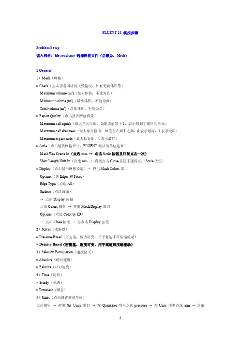
FLUENT 12 模拟步骤Problem Setup读入网格：file read case 选择网格文件（后缀为。

Mesh）1 General1）Mesh（网格）> Check（点击查看网格的大致情况，如有无负体积等）Maximum volume (m3)（最大体积，不能为负）Minimum volume (m3)（最小体积，不能为负）Total volume (m3)（总体体积，不能为负）> Report Quality（点击报告网格质量）Maximum cell squish（最大单元压扁，如果该值等于1，表示得到了很坏的单元）Maximum cell skewness（最大单元扭曲，该值在0到1之间，0表示最好，1表示最坏）Maximum aspect ratio（最大长宽比，1表示最好）> Scale（点击缩放网格尺寸，FLUENT默认的单位是米）Mesh Was Create In（点选mm →点击Scale按钮且只能点击一次）V iew Length Unit In（点选mm →直接点击Close按钮不能再点击Scale按钮）> Display（点击显示网格设定）→弹出Mesh Colors窗口Options（选Edges和Faces）Edge Type（点选All）Surface（点选曲面）→点击Display按钮点击Colors按钮→弹出Mesh Display窗口Options（点选Color by ID）→点击Close按钮→再点击Display按钮2）Solver（求解器）> Pressure-Based（压力基，压力可变，用于低速不可压缩流动）> Density-Based（密度基，密度可变，用于高速可压缩流动）3）V elocity Formulation（速度格式）> Absolute（绝对速度）> Relative（相对速度）4）Time（时间）> Steady（稳态）> Transient（瞬态）5）Units（点击设置变量单位）点击按钮→弹出Set Units窗口→在Quantities项里点选pressure →在Units项里点选atm →点击New按钮→点击OK按钮→点击Close按钮2 Models（物理模型）1）Multiphase（多相流模型）2）Energy（能量方程，一般要双击勾选）3）Viscous（粘性模型，一般选k-ε模型，所有参数保持默认设置）4）Radiation（辐射模型）5）Heat Exchanger（传热模型）6）Species（组分模型）7）Discrete Phase（离散相模型）8）Solidification & Melting（凝固与融化模型）9）Acoustics（声学模型，一般选择Broadband Noise Source模型，所有参数保持默认设置）3 Materials（定义材料）1）点击FLUENT Database →在FLUENT Fluid Materials里选择所需要的物质→点击Copy按钮→点击Close按钮→再点击Change/Create按钮2）点击User-Defined Database →选定写好的自定义文件→点击OK按钮3）自定义材料物性参数：在Name文本框中输入自定义材料名字gas →Chemical Formula文本框删除为空→修改Properties中各参数的值→点击Change/Creat e按钮→弹出Change/Create mixture and Overwrite air对话框→点击NO按钮→点击Close按钮4 Phases（相）5 Cell Zone Conditions（单元区域条件）点击Edit按钮→在Material Name项的下拉列表中选择gas（工作介质）→点击OK按钮6 Boundary Conditions（边界条件）1）Pressure-Inlet（压力进口）> Momentum（动量）Reference Frame（参考系）Gauge Total Pressure（总表压）Supersonic/Initial Gauge Pressure（初始表压或静压，一般比总表压小500Pa左右，或设为出口表压）Direction Specification Method（进口流动方向指定方法，Normal to Boundary垂直边界）Turbulence > Specification Method（湍流指定方法，Intensity and Hydraulic Diameter）Turbulent Intensity（湍流强度，一般为1）Hydraulic Diameter（水力半径，一般为管内径）> Thermal（热量）Total Temperature（总温）> Species（组分）2）Pressure -Outlet（压力出口）> Momentum（动量）Gauge Pressure（表压）Backflow Direction Specification Method（回流方向指定方法）Radial Equilibrium Pressure Distribution（径向平衡压力分布）Target Mass Flow Rate（目标质量流率）Non-Reflecting Boundary（非反射边界）Turbulence > Specification Method（湍流指定方法，点选Intensity and Hydraulic Diameter）Backflow Turbulent Intensity（回流湍流强度，一般为1）Backflow Hydraulic Diameter（回流水力半径，一般为管内径）> Thermal（热量）Backflow Total Temperature（回流总温）> Species（组分）7 Mesh Interfaces（分界面网格）8 Reference V alues（参考值）9 Adapt（自适应）Adapt →Gradient（压力梯度自适应）> Options（显示选项）Refine（加密，勾选）Coarsen（粗糙，勾选）Normalize（正规化）> Method（方法）Curvature（曲率）Gradient（梯度，勾选）Iso-V alue（等值）> Gradient of（梯度变量）Pressure（压力，点选）Static pressure（静压，点选）> Normalization（正常化）Standard（标准）Scale（可缩放，勾选）Normalize（使正常化）> Coarsen Threshold（粗糙比，0.3）> Refine Threshold（细化比，0.7）> Dynamic（动态）Dynamic（动态，勾选）Interval（每隔几次迭代自适应一次）→点击Mark按钮→点击Adapt按钮→（点击Compute按钮）→点击Apply按钮Solution1 Solution Methods（求解方法）1）Formulation（求解格式，默认为隐式Implicit）2）Flux Type（通量类型，默认为Roe-FDS）3）Gradient（求解格式，默认为Least Squares Cell Based）4）Flow（流动，点选二阶迎风格式Second Order Upwind）5）Turbulent Kinetic Energy（湍动能，点选二阶迎风格式Second Order Upwind）6）Turbulent Dissipation Rate（湍流耗散率，点选二阶迎风格式Second Order Upwind）2 Solution Controls1）Courant Number（库朗数，控制时间步长，瞬态计算才需要设置）2）Un-Relaxation Factors（欠松弛因子）> Turbulent Kinetic Energy（湍动能，默认为0.8）> Turbulent Dissipation Rate（湍流耗散率，默认为0.8）> Turbulent V iscosity（湍流粘度，默认为1）3）Equations（点击弹出控制方程）> Turbulence（湍流方程）> Flow（流动方程= 连续方程+ 动量方程+ 能量方程）4）Limits（点击弹出限制窗口）对某些变量使用限制值，如果计算的某个变量值小于最小限制值，则求解器就会用相应的极限取代计算值。

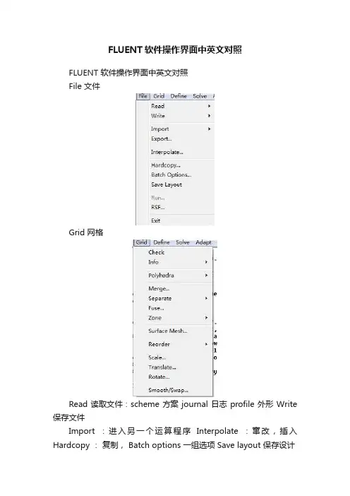
FLUENT软件操作界面中英文对照FLUENT 软件操作界面中英文对照File 文件Grid 网格Read 读取文件：scheme 方案 journal 日志 profile 外形 Write 保存文件Import ：进入另一个运算程序Interpolate ：窜改，插入Hardcopy ：复制， Batch options 一组选项 Save layout 保存设计Check 检查Info 报告：size 尺寸；memory usage 内存使用情况；zones 区域；partitions 划分存储区 Polyhedral 多面体：Convert domain 变换范围 Convert skewed cells 变换倾斜的单元 Merge 合并 Separate 分割Fuse (Merge 的意思是将具有相同条件的边界合并成一个;Fuse 将两个网格完全贴合的边界融合成内部(interior)来处理，比如叶轮机中，计算多个叶片时，只需生成一个叶片通道网格，其他通过复制后，将重合的周期边界Fuse 掉就行了。

注意两个命令均为不可逆操作，在进行操作时注意保存case)Zone 区域： append case file 添加case 文档 Replace 取代；delete 删除；deactivate 使复位；Surface mesh 表面网孔Reordr 追加，添加：Domain 范围；zones 区域；Print bandwidth 打印 Scale 单位变换 Translate 转化Rotate 旋转 smooth/swap 光滑/交换Define Models 模型：solver 解算器Pressure based 基于压力Density based 基于密度implicit 隐式，explicit 显示Space 空间：2D，axisymmetric（转动轴），axisymmetric swirl （漩涡转动轴）；Time时间：steady 定常，unsteady 非定常Velocity formulation 制定速度：absolute绝对的；relative 相对的Gradient option 梯度选择：以单元作基础；以节点作基础；以单元作梯度的最小正方形。

fluent tui使用技巧及燃烧室自动化仿真案例TUI stands for Transient User Interface and it is an interactive mode of FLUENT, a computational fluid dynamics (CFD) software developed by ANSYS. FLUENT TUI allows users to interact with the software through command line inputs instead of using the graphical user interface (GUI). Here are some tips to improve your fluency in FLUENT TUI and an example of automation simulation in a combustion chamber.1. Familiarize Yourself with FLUENT TUI: Start by learning the basic commands and syntax of FLUENT TUI. You can refer to the FLUENT documentation or online resources for a comprehensive list of commands and their functions.2. Customize and Save Commands: FLUENT TUI allows you to create custom commands and save them for future use. This can greatly simplify repetitive tasks. Use the Define/User-Defined Function (UDF) option to define custom commands and then save them for later use.3. Use Journal Files: Journal files are scripts that contain a sequence of TUI commands. You can create journal files by recording your actions in the GUI or by manually writing the commands. Using journal files can automate repetitive tasks and allow for easy reproducibility ofsimulations.4. Utilize Shortcuts: FLUENT TUI provides many shortcuts to speed up your workflow. For example, you can use the "" wildcard to select multiple objects at once, use "rp" to repeat the last command with revised parameters, or use "ac" to access the command that was previously active.5. Incorporate Macros: Macros are predefined sets of commands that can be executed with a single command. Macros can be useful for complex simulations with multiple steps or for automating a series of tasks. You can create macros by recording a set of commands or writing them manually.Example: Combustion Chamber Automation Simulation1. Load Pre-processing Data: Use the "file/read-case" command to load the pre-processing files, such as mesh file (.msh) and boundary condition files (d). Make sure to specify the correct file paths.2. Define Boundary Conditions: Set the appropriate boundary conditions for the combustion chamber, such as inlet velocity, pressure, andtemperature, and outlet pressure.3. Define Combustion Model: Choose a combustion model that suits your simulation requirements, such as a laminar or turbulent combustion model. Set the relevant parameters for the selected model using the appropriate commands.4. Perform Iterative Solver: Use the "solve/iterate" command to start the iterative solution process. Adjust the convergence criteria and maximum iterations as needed. Monitor the convergence and make adjustments if required.5. Post-processing: Once the simulation is complete, use post-processing commands to analyze and visualize the results, such as contour plots, vector plots, or exporting data for further analysis.By applying these tips and following the example, you can enhance your skills in using FLUENT TUI and automate combustion chamber simulations. Remember to refer to the documentation and practice regularly to become proficient in FLUENT TUI.。

ｐ ｕｍｐ・
Ｋ ｅ ｗ ｏ ｄｓ Ｍｕ ｔ－ ｅ ｒＰ ｍ ｐ；Ｒｅ ｅ ｓ ｇｎ ｅ ｉ ｙ ｒ ： ｌｉ ｇ ａ ｕ ｖ ｒｅ Ｅｎ ｉ ｅ ｒｎｇ；Ｆ ＬＵＥＮＴ ；Ｍ ｏ ｉ ｇ Ｇｒｄ ｖｎ ｉ
在大 型和高精 密 数控 机 床 导轨 润 滑 系统 中 ， 体 流 静压 润滑 系统通过 静压 支 承 消 除机 床 导轨 的爬行 ， 保
ｌ 多 回路 泵 数值 模 拟 的前 处 理 Ｊ
本 文采用 最 简单 的多 回路 泵 模 型—— 三 齿轮 泵 ， 多 回路泵 转速 为 ４ ５ ｒｍｉ， ９ ／ ｎ 中心轮 为 逆 时 针转 动 ， 齿 轮为标 准 渐 开 线 圆柱 齿 轮 ， 模 数 为 ２ ｍｍ， 数 为 其 齿
多个泵 的使 用性 能。为准 确掌握 多 回路泵 内部流 场 变 化 ， 用 Ｆ Ｕ Ｎ 运 Ｌ Ｅ Ｔ软 件 中 的动 网格 技术 对 多
回路泵 进行流 场动 态数值 模拟 ， 析 多回路泵 在齿 轮旋 转情 况 下 的 内部 流 场变 化 ， 分 从而 为 多 回路泵
的逆 向设计和 结构优 化奠 定基础 。 关键词 ： 回路 泵 多 逆 向设计 ＦＵ Ｎ Ｌ Ｅ Ｔ 动 网格
ｍｕ —ｇ ａ ｍｐ，ｔ ｏ ｉ ｇ ｇ ｉ ｅ ｈ ｏｏ ｙ ｉ ｌｅ ｔｓ ｆｗａ ｅ ｉ ｓ ｄ ｔ ｕ ｒｃ ｌｙ ｓｍｕ ａｅ ｔ ｅ ｆ ｗ ｈｉ ｅ ｒｐｕ ｈｅｍ ｖ ｎ ｒｄ ｔｃ ｎ ｌ ｇ ｎ ｆｕ ｎ ｏ ｔ ｒ ｓ ｕ ｅ ｏ ｎ ｍｅ ｉａｌ ｉ ｌ ｔ ｈ ｏ ｌ
Ｎｕ ｍｅ ｉａ ｍ ｕａ ｉｎ ｏ ｌｗ ｉｌ ｆＭ ｕｔ Ｃｉ ｕｔＰｕ Ｄ Ｂａ ｅ １ Ｆ ＵＥＮＴ ｒ ｌ ｃ Ｓｉ ｌｔ ｆＦｏ Ｆｅｄ ｏ ｌ— ｒ ｉ ｏ ｉ ｃ ｍ ｓ ｄ ０３ Ｌ

CFD 数值计算模型软件平台：PRO-E3.0理论上，水泵的进口到出口的流动区域就是我们的计算模型。

一般，全流场算域分为5部分：1. 叶轮进口段2. 叶轮内流动域3. 泵体前腔4. 泵体后腔5. 泵体（涡壳）6. 出口段通常我们计算的时候运用流动域1、2、5、6, 最简化的为流动域2、5.计算模型可以运用PRO-E ，UG ，CATIA 等三维造型软件，具体的造型过程和步骤请点击三维造型培训，模型通常保存为STP 和IGS 文件格式.各流动域可以分别造型，然后进行装配.简单的模型可以运用FLUENT 前处理软件GAMBIT 中进行.下图为某型号纸浆泵，计算模型包括：1. 叶轮进口段，2. 叶轮内流动域，3. 泵体前腔，4. 泵体后腔，5. 泵体（涡壳）某型号纸浆泵计算模型下图为某型号低比速离心泵计算模型，包括：1. 叶轮内流动域，2. 泵体（涡壳）。

模型作了简化，没有考虑腔体中的流动。

某型号低比速离心泵计算模型下图为某型号的循环泵全流场计算模型，包括所有的流动区域。

某型号循环泵计算模型计算模型的造型是CFD 工作中非常重要的一部分，由于造型可能影响到网格划分和网格生成质量，因此，科学合理的造型将达到事半功倍的效果。

网格划分计算模型导入步骤 File--Import, 见下图。

导入计算模型, 轮廓图见下图。

网格划分界面a 面合并界面b 网格分界面c 网格质量检查模型处理好后, 分别对流动区域进行网格划分通常, 叶轮和泵体的几何现状不规则，运用T-Grid 类型进行网格划分，网格间距根据模型大小和计算机性能配置进行设置，一般取1-10.在进行全流场计算时，您可以在口环、涡壳隔舌、压力梯度大的区域进行局部加密，局部加密时，需要注意网格变化不能太剧烈。

为了提高计算精度和粘性底层的影响，先画好边界层网格，再画体网格。

在FLUENT 中，您可以根据计算的结果，用Adapt-Gradient 对压力梯度大的区域进行加密，如下图所示。

Fluent专业词汇大全流体动力学 fluid dynamics连续介质力学 mechanics of continuous media介质 medium流体质点 fluid particle无粘性流体 nonviscous fluid, inviscid fluid连续介质假设 continuous medium hypothesis流体运动学 fluid kinematics水静力学 hydrostatics液体静力学 hydrostatics支配方程 governing equation分步法 fractional step method伯努利定理 Bernonlli theorem毕奥-萨伐尔定律 Biot-Savart law欧拉方程 Euler equation亥姆霍兹定理 Helmholtz theorem开尔文定理 Kelvin theorem涡片 vortex sheet库塔-茹可夫斯基条件 Kutta-Zhoukowski condition 布拉休斯解Blasius solution达朗贝尔佯廖 d'Alembert paradox雷诺数 Reynolds number施特鲁哈尔数 Strouhal number随体导数 material derivative不可压缩流体 incompressible fluid质量守恒 conservation of mass动量守恒 conservation of momentum能量守恒 conservation of energy动量方程 momentum equation 能量方程 energy equation控制体积 control volume液体静压 hydrostatic pressure 涡量拟能 enstrophy压差 differential pressure流[动] flow流线 stream line流面 stream surface流管 stream tube迹线 path, path line流场 flow field流态 flow regime流动参量 flow parameter流量 flow rate, flow discharge 涡旋 vortex涡量 vorticity涡丝 vortex filament涡线 vortex line涡面 vortex surface涡层 vortex layer涡环 vortex ring涡对 vortex pair涡管 vortex tube涡街 vortex street卡门涡街 Karman vortex street 马蹄涡 horseshoe vortex对流涡胞 convective cell卷筒涡胞 roll cell涡 eddy涡粘性 eddy viscosity环流 circulation环量 circulation速度环量 velocity circulation偶极子 doublet, dipole驻点 stagnation point总压[力] total pressure总压头 total head静压头 static head总焓 total enthalpy能量输运 energy transport速度剖面 velocity profile库埃特流 Couette flow单相流 single phase flow单组份流 single-component flow均匀流 uniform flow非均匀流 nonuniform flow二维流 two-dimensional flow三维流 three-dimensional flow准定常流 quasi-steady flow非定常流unsteady flow, non-steady flow 暂态流transient flow周期流 periodic flow振荡流 oscillatory flow分层流 stratified flow无旋流 irrotational flow有旋流 rotational flow轴对称流 axisymmetric flow不可压缩性 incompressibility不可压缩流[动] incompressible flow浮体 floating body定倾中心 metacenter阻力 drag, resistance减阻 drag reduction表面力 surface force表面张力 surface tension毛细[管]作用 capillarity来流 incoming flow自由流 free stream自由流线 free stream line外流 external flow进口 entrance, inlet出口 exit, outlet扰动 disturbance, perturbation分布 distribution传播 propagation色散 dispersion弥散 dispersion附加质量 added mass ,associated mass 收缩 contraction镜象法 image method无量纲参数 dimensionless parameter 几何相似 geometric similarity运动相似 kinematic similarity动力相似[性] dynamic similarity平面流 plane flow势 potential势流 potential flow速度势 velocity potential复势 complex potential复速度 complex velocity流函数 stream function源 source汇 sink速度[水]头 velocity head拐角流 corner flow空泡流 cavity flow超空泡 supercavity超空泡流 supercavity flow空气动力学 aerodynamics低速空气动力学low-speed aerodynamics 高速空气动力学high-speed aerodynamics 气动热力学 aerothermodynamics 亚声速流[动] subsonic flow跨声速流[动] transonic flow超声速流[动] supersonic flow锥形流 conical flow楔流 wedge flow叶栅流 cascade flow非平衡流[动] non-equilibrium flow细长体 slender body细长度 slenderness钝头体 bluff body钝体 blunt body翼型 airfoil翼弦 chord薄翼理论 thin-airfoil theory构型 configuration后缘 trailing edge迎角 angle of attack失速 stall脱体激波 detached shock wave波阻 wave drag诱导阻力 induced drag诱导速度 induced velocity临界雷诺数 critical Reynolds number前缘涡 leading edge vortex附着涡 bound vortex约束涡 confined vortex气动中心 aerodynamic center气动力 aerodynamic force气动噪声 aerodynamic noise气动加热 aerodynamic heating离解 dissociation地面效应 ground effect气体动力学 gas dynamics稀疏波 rarefaction wave热状态方程 thermal equation of state喷管 Nozzle普朗特-迈耶流 Prandtl-Meyer flow瑞利流 Rayleigh flow可压缩流[动] compressible flow可压缩流体 compressible fluid绝热流 adiabatic flow非绝热流 diabatic flow未扰动流 undisturbed flow等熵流 isentropic flow匀熵流 homoentropic flow兰金-于戈尼奥条件 Rankine-Hugoniot condition 状态方程 equation of state量热状态方程 caloric equation of state 完全气体 perfect gas 拉瓦尔喷管 Laval nozzle马赫角 Mach angle马赫锥 Mach cone马赫线 Mach line马赫数 Mach number马赫波 Mach wave当地马赫数 local Mach number冲击波 shock wave激波 shock wave正激波 normal shock wave斜激波 oblique shock wave头波 bow wave附体激波 attached shock wave激波阵面 shock front激波层 shock layer压缩波 compression wave反射 reflection折射 refraction散射 scattering衍射 diffraction绕射 diffraction出口压力 exit pressure超压[强] over pressure反压 back pressure爆炸 explosion爆轰 detonation缓燃 deflagration水动力学 hydrodynamics液体动力学 hydrodynamics泰勒不稳定性 Taylor instability盖斯特纳波 Gerstner wave斯托克斯波 Stokes wave瑞利数 Rayleigh number自由面 free surface波速 wave speed, wave velocity 波高 wave height波列 wave train波群 wave group波能 wave energy表面波 surface wave表面张力波 capillary wave规则波 regular wave不规则波 irregular wave浅水波 shallow water wave深水波 deep water wave重力波 gravity wave椭圆余弦波 cnoidal wave潮波 tidal wave涌波 surge wave破碎波 breaking wave船波 ship wave非线性波 nonlinear wave孤立子 soliton水动[力]噪声 hydrodynamic noise 水击 water hammer空化 cavitation空化数 cavitation number空蚀 cavitation damage超空化流 supercavitating flow水翼 hydrofoil水力学 hydraulics洪水波 flood wave涟漪 ripple消能 energy dissipation海洋水动力学 marine hydrodynamics 谢齐公式 Chezy formula 欧拉数 Euler number弗劳德数 Froude number水力半径 hydraulic radius水力坡度 hvdraulic slope高度水头 elevating head水头损失 head loss水位 water level水跃 hydraulic jump含水层 aquifer排水 drainage排放量 discharge壅水曲线 back water curve压[强水]头 pressure head过水断面 flow cross-section明槽流 open channel flow孔流 orifice flow无压流 free surface flow有压流 pressure flow缓流 subcritical flow急流 supercritical flow渐变流 gradually varied flow急变流 rapidly varied flow临界流 critical flow异重流 density current, gravity flow堰流 weir flow掺气流 aerated flow含沙流 sediment-laden stream降水曲线 dropdown curve沉积物 sediment, deposit沉[降堆]积 sedimentation, deposition沉降速度 settling velocity流动稳定性 flow stability不稳定性 instability奥尔-索末菲方程 Orr-Sommerfeld equation 涡量方程 vorticity equation泊肃叶流 Poiseuille flow奥辛流 Oseen flow剪切流 shear flow粘性流[动] viscous flow层流 laminar flow分离流 separated flow二次流 secondary flow近场流 near field flow远场流 far field flow滞止流 stagnation flow尾流 wake [flow]回流 back flow反流 reverse flow射流 jet自由射流 free jet管流 pipe flow, tube flow内流 internal flow拟序结构 coherent structure猝发过程 bursting process表观粘度 apparent viscosity运动粘性 kinematic viscosity动力粘性 dynamic viscosity泊 poise厘泊 centipoise厘沱 centistoke剪切层 shear layer次层 sublayer流动分离 flow separation层流分离 laminar separation湍流分离 turbulent separation分离点 separation point附着点 attachment point再附 reattachment再层流化 relaminarization起动涡 starting vortex驻涡 standing vortex涡旋破碎 vortex breakdown涡旋脱落 vortex shedding压[力]降 pressure drop压差阻力 pressure drag压力能 pressure energy型阻 profile drag滑移速度 slip velocity无滑移条件 non-slip condition壁剪应力 skin friction, frictional drag 壁剪切速度 friction velocity磨擦损失 friction loss磨擦因子 friction factor耗散 dissipation滞后 lag相似性解 similar solution局域相似 local similarity气体润滑 gas lubrication液体动力润滑 hydrodynamic lubrication 浆体 slurry泰勒数 Taylor number纳维-斯托克斯方程Navier-Stokes equation 牛顿流体Newtonian fluid边界层理论 boundary later theory边界层方程 boundary layer equation边界层 boundary layer附面层 boundary layer层流边界层 laminar boundary layer湍流边界层 turbulent boundary layer温度边界层 thermal boundary layer边界层转捩 boundary layer transition边界层分离 boundary layer separation边界层厚度 boundary layer thickness位移厚度 displacement thickness动量厚度 momentum thickness能量厚度 energy thickness焓厚度 enthalpy thickness注入 injection吸出 suction泰勒涡 Taylor vortex速度亏损律 velocity defect law形状因子 shape factor测速法 anemometry粘度测定法 visco[si] metry流动显示 flow visualization油烟显示 oil smoke visualization孔板流量计 orifice meter频率响应 frequency response油膜显示 oil film visualization阴影法 shadow method纹影法 schlieren method烟丝法 smoke wire method丝线法 tuft method氢泡法 nydrogen bubble method相似理论 similarity theory相似律 similarity law部分相似 partial similarity定理 pi theorem, Buckingham theorem 静[态]校准 static calibration动态校准 dynamic calibration风洞 wind tunnel激波管 shock tube激波管风洞 shock tube wind tunnel水洞 water tunnel拖曳水池 towing tank旋臂水池 rotating arm basin扩散段 diffuser测压孔 pressure tap皮托管 pitot tube普雷斯顿管 preston tube斯坦顿管 Stanton tube文丘里管 Venturi tubeU形管 U-tube压强计 manometer微压计 micromanometer多管压强计 multiple manometer静压管 static [pressure]tube流速计 anemometer风速管 Pitot- static tube激光多普勒测速计 laser Doppler anemometer, laser Doppler velocimeter热线流速计 hot-wire anemometer热膜流速计 hot- film anemometer流量计 flow meter粘度计 visco[si] meter涡量计 vorticity meter传感器 transducer, sensor压强传感器 pressure transducer热敏电阻 thermistor示踪物 tracer时间线 time line脉线 streak line尺度效应 scale effect壁效应 wall effect堵塞 blockage堵寒效应 blockage effect动态响应 dynamic response响应频率 response frequency底压 base pressure菲克定律 Fick law巴塞特力 Basset force埃克特数 Eckert number格拉斯霍夫数 Grashof number努塞特数 Nusselt number普朗特数 prandtl number雷诺比拟 Reynolds analogy施密特数 schmidt number斯坦顿数 Stanton number对流 convection自由对流 natural convection, free convec-tion 强迫对流 forced convection热对流 heat convection质量传递 mass transfer传质系数 mass transfer coefficient热量传递 heat transfer传热系数 heat transfer coefficient对流传热 convective heat transfer辐射传热 radiative heat transfer动量交换 momentum transfer能量传递 energy transfer传导 conduction热传导 conductive heat transfer热交换 heat exchange临界热通量 critical heat flux浓度 concentration扩散 diffusion扩散性 diffusivity扩散率 diffusivity扩散速度 diffusion velocity分子扩散 molecular diffusion沸腾 boiling蒸发 evaporation气化 gasification凝结 condensation成核 nucleation计算流体力学 computational fluid mechanics多重尺度问题 multiple scale problem伯格斯方程 Burgers equation对流扩散方程 convection diffusion equationKDU方程 KDV equation修正微分方程 modified differential equation拉克斯等价定理 Lax equivalence theorem数值模拟 numerical simulation大涡模拟 large eddy simulation数值粘性 numerical viscosity非线性不稳定性 nonlinear instability希尔特稳定性分析 Hirt stability analysis相容条件 consistency conditionCFL条件 Courant- Friedrichs- Lewy condition ,CFL condition 狄里克雷边界条件 Dirichlet boundarycondition熵条件 entropy condition远场边界条件 far field boundary condition流入边界条件 inflow boundary condition无反射边界条件nonreflecting boundary condition数值边界条件 numerical boundary condition流出边界条件 outflow boundary condition冯.诺伊曼条件 von Neumann condition近似因子分解法 approximate factorization method人工压缩 artificial compression人工粘性 artificial viscosity边界元法 boundary element method配置方法 collocation method能量法 energy method有限体积法 finite volume method流体网格法 fluid in cell method, FLIC method通量校正传输法 flux-corrected transport method通量矢量分解法 flux vector splitting method伽辽金法 Galerkin method积分方法 integral method标记网格法 marker and cell method, MAC method特征线法 method of characteristics直线法 method of lines矩量法 moment method多重网格法 multi- grid method板块法 panel method质点网格法 particle in cell method, PIC method质点法 particle method预估校正法 predictor-corrector method投影法 projection method准谱法 pseudo-spectral method随机选取法 random choice method激波捕捉法 shock-capturing method激波拟合法 shock-fitting method谱方法 spectral method稀疏矩阵分解法 split coefficient matrix method不定常法 time-dependent method时间分步法 time splitting method变分法 variational method涡方法 vortex method隐格式 implicit scheme显格式 explicit scheme交替方向隐格式alternating direction implicit scheme, ADI scheme 反扩散差分格式 anti-diffusion difference scheme 紧差分格式 compact difference scheme守恒差分格式 conservation difference scheme克兰克-尼科尔森格式 Crank-Nicolson scheme杜福特-弗兰克尔格式 Dufort-Frankel scheme指数格式 exponential scheme戈本诺夫格式 Godunov scheme高分辨率格式 high resolution scheme拉克斯-温德罗夫格式 Lax-Wendroff scheme蛙跳格式 leap-frog scheme单调差分格式 monotone difference scheme保单调差分格式 monotonicity preserving diffe-rence scheme 穆曼-科尔格式 Murman-Cole scheme半隐格式 semi-implicit scheme斜迎风格式 skew-upstream scheme全变差下降格式total variation decreasing scheme TVD scheme 迎风格式 upstream scheme , upwind scheme 计算区域 computational domain物理区域 physical domain影响域 domain of influence依赖域 domain of dependence区域分解 domain decomposition维数分解 dimensional split物理解 physical solution弱解 weak solution黎曼解算子 Riemann solver守恒型 conservation form弱守恒型 weak conservation form强守恒型 strong conservation form散度型 divergence form贴体曲线坐标 body- fitted curvilinear coordi-nates [自]适应网格 [self-] adaptive mesh适应网格生成 adaptive grid generation自动网格生成 automatic grid generation 数值网格生成 numerical grid generation 交错网格 staggered mesh网格雷诺数 cell Reynolds number数植扩散 numerical diffusion数值耗散 numerical dissipation数值色散 numerical dispersion数值通量 numerical flux放大因子 amplification factor放大矩阵 amplification matrix阻尼误差 damping error离散涡 discrete vortex熵通量 entropy flux熵函数 entropy function伯努利方程 Bernoulli equation。

可扩展性
支持与其他CAD、CAE软件的集成，方便数 据交换和协同工作。
02
Fluent软件基础
Fluent软件界面介绍
工具栏
提供常用命令的快 捷方式。
导航栏
提供视图切换、模 型设置等操作。
菜单栏
包含文件、编辑、 查看等常用菜单选 项。
图形窗口
显示计算域的几何 形状和计算结果。
属性面板
设置材料属性、边 界条件等参数。
详细描述
湍流模型的选择应根据流动特性、计算资源和模拟需求进行权衡。常见的湍流模 型包括标准k-ε模型、修正k-ε模型、SST k-ω模型、Realizable k-ε模型等。在选 择模型时，需要考虑模型的适用范围、精度和计算效率。
多相流模型选择与设置
总结词
多相流模拟在工程领域具有广泛的应用，选择合适的多相流模型能够准确模拟多相流动的物理特性。
适用于模拟多相流体的流动， 如气液、液液等。
化学反应模拟
可以对流体中的化学反应进行 模拟，如燃烧过程等。
Fluent软件的特点和优势
强大的计算能力
采用先进的数值计算方法，能够处理大规模 的流体动力学问题。
易用性
界面友好，操作简单，方便用户快速上手。
丰富的物理模型
内置多种物理模型，满足不同领域的模拟需 求。
版本发展
随着技术的不断进步，Fluent软件的版本也在不断更 新，功能越来越强大。
适用领域
广泛应用于航空航天、汽车、能源、环境等众多领域 。
Fluent软件的应用领域
流体动力学模拟
Fluent软件最核心的应用领域 ，可以对流体进行三维流动模
拟。
传热分析
可以模拟流体中的热量传递过 程，进行热分析。

CFD软件Fluent在多级泵内部流场数值分析中的应用摘要：随着我国经济实力的不断上升，计算机信息化水平也我国多个领域有着广泛的应用，本文则主要分析多级泵内部流场中CFD软件Fluent对其的应用，经研究得知，采用这种数值计算方法改型优化，提高多级泵内部流场分析效率，也是计算流体力学和计算机技术的一大融合，值的推广和应用。

关键词：Fluent；多级泵；内部流场；数值分析；在石化、农业、矿业及电业等领域都涉及多级泵，因它自身扬程高，占地小等优点而被广泛应用。

对多级泵内部流动规律进行分析，多提高多级泵的运行和设计有着现实意义。

随着计算机技术的不断发展，采用数值来分析多级泵内部流场，并预测了效率和扬程，这些都为多级泵内部流场分析，及提高效率和改型优化起到参考价值作用。

本文就利用CFD软件Fluent对多级泵内场速度和压力进行三维数据模型，并加以对比分析。

1. Fluent相关概述目前国际上比较流行的商用CFD软件包则是Fluent，在美国的市场占有率为60%。

凡是流体、热传递和化学反应有关的工业领域都是涉及。

其自身丰富的物理模型，先进的数值方法和强大的前后处理功能，让它在汽车设计、航空航天及石油天燃气等方面都有广泛的应用。

Fluenth系列软件包括通用的CFD软件FLUENT、POLY&shy；FLOW、FIDAP，CFD教学软件FlowLab，工程设计软件FloWizard、FLUENT for CATIA V5，TGrid、G/Turbo。

Fluen软件包含非常丰富，经过工程确认的物理模型，高超音速流场、转捩、传热与相变、化学反应与燃烧、多相流、旋转机械、动/变形网格、噪声、材料加工等复杂机理的流动问题都可进行模拟。

这款软件有以下几个特点：1）适用面广；各种物理模型都可优化，如：辐射模型，相变模型，反应流模型，离散相变模型，计算流体流动和热传导模型，多相流模型及化学组分输运。

它的数值解法好可适用于每一种物理问题的流动特点，用户可自行选择它的显示或隐式差分格，在计算速度、精度及稳定性方面都可达到效果最佳。

基于Fluent的多回路齿轮泵虚拟样机设计摘要：多齿轮泵因为能稳定的供给各润滑点等量的油液，为数控机床导轨提供静压支撑，被广泛应用于大型高精密加工的数控机床中。

利用虚拟样机技术在计算机上建立多齿轮泵的数学模型，同时采用FLUETN软件对模型进行模拟仿真，有利于减少产品研发周期，降低研发成本。

关键词：多齿轮泵；虚拟样机；Fluent；模拟仿真Design Of Virtual Prototyping Of Multi-Gear Pump Based OnFluent(DaLian JiaoTong University DaLian City LiaoNing Province Postal Code：116028 ) Abstract: The Multi-gear pump is widely used in the high-precision machining of the NC machine tools, because it can afford equal amounts of oil to each lubricant point stably and the hydrostatic pressure lubricating system for the machine tool guide ways. The Virtual Prototyping can build the mathematical model of the Multi-gear pump on the computer, and use the software FLUENT to analog simulation. This will help to reduce the development cycle of the product and lower the costs.Keywords：Multi-gear pump；Virtual Prototyping；Fluent；analog simulation0 引言虚拟样机技术（Virtual Prototyping，简称VP）是一种以计算机建模、仿真为基础上的数字化设计方法，兴起于20世纪80年代，90年代开始发展起来，目前已被广泛应用于制造业中。

Tutorial: Simulating a Gear Pump Using Dynamic Mesh with 2.5D Re-meshingIntroductionThe purpose of this tutorial is to demonstrate how to simulate a gear pump using the dynamic mesh model in Fluent. A prescribed rotation rate is applied to the two gears using a UDF macro. There is significant displacement of the valve and hence re-meshing approach is used in conjunction with smoothing. The mesh in the zone where the gears are located is a 2D triangular mesh which is expanded, or extruded, along the normal axis of the dynamic zone. The triangular surface mesh is re-meshed and smoothed on one side, and the changes are then extruded to the opposite side. The opposite side of the triangular mesh is assigned to be a deforming zone with only smoothing enabled. This tutorial uses the workbench workflow for solving the problem.This tutorial demonstrates how to do the following:Set up a problem using the 2.5D dynamic re-meshing model.Specify dynamic mesh modeling parameters.Specify a rigid body motion zone.Specify a deforming zone.Use prescribed motion UDF macro.Perform the calculation with residual plotting.Post process using CFD-PostParametrization is demonstrated in the AppendixPrerequisitesThis tutorial assumes that you are familiar with the FLUENT interface and have completed Tutorial 1 from the FLUENT 13.0 Tutorial Guide. You should also be familiar with the dynamic mesh model. Referto Section 11.7: Steps in Using Dynamic Meshes in the FLUENT 13.0 User's Guide for more information on the use of the dynamic mesh model.Problem DescriptionThe problem considered is shown schematically in Figure 1. A gear pump uses the meshing of gears to pump fluid by displacement. They are one of the most common types of pumps for hydraulic fluid power applications. The current setup is an external gear pump which uses two external spur gears. As the gears rotate they separate on the intake side of the pump, creating a void and suction which is filled by fluid. The fluid is carried by the gears to the discharge side of the pump, where the meshing of the gears displaces the fluid.The gears in this tutorial are made to rotate at a constant rate of 100 rad/s. The fluid being pumped in oil with a density of 844 kg/m3 and viscosity of 0.02549 kg/m-s. Fluid is sucked in from the inlet side and pumped out though the outlet side by rotation of the gears. The mass flow rate of fluid in and out of the pump is of interest.Figure 1:Problem schematicPreparation1.Open Workbench 13.02.Unzip the project gear_pump.wbpz by File -> Restore Archive3.Double click on the Fluent Setup CellFigure 2:Workbench project page4.From the FLUENT launcher, start FLUENT.Setup and SolutionStep 1: Mesh1.The mesh is automatically read into Fluent and displayed in the graphics window.2.Note that if you are using standalone Fluent, you can read in the mesh from the File menu: File ->Read -> Mesh. The mesh file for this project can be accessed by navigating the project files to "gear_pump_files\dp0\FFF\MECH". The mesh file is named FFF.msh.Figure 3:Fluent window and mesh display3.Check the mesh by clicking on Mesh -> Check4.FLUENT will perform various checks on the mesh and report the progress in the console. Makesure that the minimum volume reported is a positive number.5.Note that Most of the Fluent settings can be accessed by navigating the setup tree on the left inthe Fluent WindowStep 2:General SettingsProblem Setup -> General Settings1.Enable time-dependent calculations.(a)Select Transient from the Time list.Figure 4:General settingsStep 3: ModelsProblem Setup -> Models -> Viscous1.Enable the Realizable k-epsilon model with standard wall functions. For classes of problems thatinvolve rotation, boundary layers under strong adverse pressure gradients, separation, and recirculation, this model shows superior performance over the standard k-epsilon model.Figure 5:Viscous models window Step 4: MaterialsProblem Setup -> Materials1.Create/Edit(a)Type in material name as "oil"(b)Enter density to be 844 kg/m3(c)Enter viscosity to be 0.02549 kg/m-s(d)Change/Create(e)Create mixture and overwrite air? Click on "Yes"2.Close the Materials panel.Figure 6:Materials panelStep 5: Cell Zone ConditionsProblem Setup -> Cell Zone Conditions1.Pick each cell zone listed and click Create/Edit2. In the pop up window, make sure each cell zone is of Type Fluid and that the material selected isoil.Step 6: Boundary ConditionsProblem Setup -> Boundary ConditionsIn this step, you will set the inlet and outlet conditions.1. Define boundary conditions for the inlet zone.(a)Pick the boundary named as "inlet" and switch the Type to pressure-inlet(b)Maintain defaults and click OK to close the panel2.Similarly pick the outlet zone and click Edit(a)Set the outlet Gauge pressure to be 101325 Pa (~ 1atm)(b)Maintain defaults for everything else and click OK to close the panel3.Close the Boundary Conditions panel.Note: Many inputs to the Fluent model can be parametrized for what if studies or DOE studies (See Appendix for steps).Step 7: Compile the UDFNote that the tutorial project has the UDF libraries included. The UDF has been compiled in serial on Windows 64 bit machine. To run the tutorial on any other hardware specification, it needs to be re-compiled.The gears are set to rotate in opposite directions at a constant rotation rate of 100 rad/s in the UDF macro.A UDF is used in this example. The DEFINE_CG_MOTION macro is used to define the rotation on each gear. You will need a c-compiler installed on your machine to be able to compile UDFs.Define -> User Defined -> Functions -> Compiled1.Click the Add... button in the Source Files group box.2.The Select File dialog will open.3.Browse to the folder "check_valve_diffusion_3d_files\dp0\FFF\Fluent". Select the filegearpump.c and click OK to close the Select File dialog.4. Click Build to build the library.5. FLUENT will set up the directory structure and compile the code. The compilation will bedisplayed in the console.6. Click Load to load the library.7.Close the Compiled UDFs panel.Figure 7:Compiled UDF panelStep 8: Mesh Motion Setup1.Enable dynamic mesh motion and specify the associated parameters.(a)Problem Setup -> Dynamic Mesh(b)Enable Dynamic Mesh in the Models group box.(c)Enable Smoothing and Remeshing in the Mesh Methods group box.(d)Click on Mesh Method Settings to open the Mesh Method Settings panel and turn on the2.5D remeshing method in the Remeshing tab.(e)Click on "Use Defaults" to set the minimum and maximum length scales(f)Set Size Remeshing Interval to 1.Figure 8:Dynamic mesh settings 2. Specify the motion of the gearl(a)Click on Create/Edit in the Dynamic Mesh Panel.(b)Select gear1 from the Zone Names drop-down list.(c)Retain the selection of Rigid Body in the Type list.(d)Select gear1::libudf from the Motion UDF/Profile drop down list.(e)Enter Center of Gravity location of the gear as (X, Y, Z) = (0.0, 0.085, 5.0e-3) m(f)Click Create.Figure 9:Settings for 6DOF ball valve(g)FLUENT will create the dynamic zone gear1 which will be available in the DynamicZones list.3.Do the same for gear2 with gear2"libudf hooked to the Motion UDF panel and (0.0,-0.085,5.0e-3)as center of gravity.4.Specify the motion of the symmetry1-gear_fluid.Figure 10:Geometry definition for symmetry1-gear_fluid(a)Select symmetry1-gear_fluid from the Zone Names drop-down list.(b)Select Deforming from the Type list.(c)In the Geometry definition tab, turn Definition to plane, specify point on the plane as(0.0,0.0,0.01) m and the plane normal as (0,0,1). This ensures that re-meshing does notcause the mesh to move out of the specified plane.(d)Click the Meshing Options tab and set the following parameters:(e)Enable Smoothing and Remeshing in the Methods group box.(f)Specify Minimum and Maximum length scales as 0.0005 and 0.002 respectively. The"Zone Scale Info" button gives information on the minimum and maximum length scales in the domain and can be used as a guide to set the above values.(g)The Maximum skewness is set to 0.8.(h)Click Create.(i)FLUENT will create the dynamic zone symmetry1-gear_fluid which will be available inthe Dynamic Zones list.5.Do the same for symmetry2-gear_fluid(a)For the zone, in the Meshing Options tab be sure to turn off Remeshing and enable onlySmoothing.(b)In Geometry Definition tab, the point on the plane is (0,0,0) with plane normal (0,0,1).6.Close the Dynamic Mesh Zones panel.7.Save the project.Figure 11:Meshing Options for symmetry2-gear_fluid8.Displaying the Zone Motion(a)Click on Display Zone Motion button in the Dynamic Mesh Panel(b)Enter time step size to be 5e-6(c)Number of steps is 1000(d)Integrate(e)In Preview Controls, again set time step to 5e-6(f)Number of steps to 1000(g)Preview(h)This shows the rotation of the zone as a preview. This helps to make sure that the UDF isspecifying the motion of the zone correctly.9.Similarly, the mesh motion can be displayed(a)Click on Preview Mesh Motion(b)Display the mesh on the geometry by going to Graphics and Anomations -> Mesh->Setup(c)Enter time step size to be 5e-6(d)Number of time steps 50(e)Preview(f)This shows the gears motion and remeshing for the specified number of time steps.(g)The mesh is now in a deformed state. Before starting calculation, close Fluent and re-open by clicking on the setup cell again. This ensures that the mesh is re-read as it waswritten out from the meshing application.Figure 12:Previewing the mesh motionStep 9:SolutionIn a dynamic mesh simulation, the mesh changes are saved in the case files. At any point in the solution, to revert the mesh back to original settings and to start calculation from beginning, close Fluent and click on the Settings cell again in the project page. This will re-launch Fluent with the original mesh but with all the saved settings. To re-start a calculation, always launch Fluent from the Solution cell. This reads in the latest Fluent case and data file.1.Request saving of case and data files every 500 time steps.(a)Solution -> Calculation Activities -> Autosave(b)Enter 500 for both Autosave Case File Frequency and Autosave Data File Frequency.Clicking on Edit makes more options available.(c)Click OK to close the Autosave panel.2.Write out CFD-Post compatible files for transient data post processing in the interests ofminimizing hard disk space,(a)Calculation Activities > Automatic Export > Create > Solution Data Export.(b)Choose file type to be CFD-Post compatible.(c)Select Frequency to be 100(d)Give a file name ./gearpump. Adding ./ at the beginning of the file name ensures that it iswritten out in the current working directory.(e)Select (Statis Pressure, Velocity Magnitude, X Velocity, Y Velocity, Z Velocity, X-Coordinate, Y-Coordinate, Z-Coordinate and Density as variables to post process)(f)OK3.Solution -> Solution Methods(a)Retain defaults4.Solution -> Solution Controls(a)Change Under-Relaxation factors of Pressure to 0.4, Momentum to 0.5, TurbulentKinetic Energy to 0.7, Turbulent Dissipation Rate to 0.7 and Turbulent Viscosity to 0.75.(b)This is done because when running the solution it was found that the solution process ismore stable with these URFs.5.Enable the plotting of residuals during the calculation.(a)Solution -> Monitors -> Residual(b)Enable Plot in the Options group box.(c)Click OK to close the Residual Monitors panel.6.Setup a Surface Monitor to track the mass flow rate at the outlet of the pump(a)Monitors -> Surface Monitors -> Create(b)Select Report Type to be Mass Flow Rate(c)Select Surface to be outlet(d)Enable Plot and Write OptionsFigure 13:Setting Surface Monitors(e)Select X-Axis to be Flow Time(f)Get Data Every 1 Time Step(g)Name the surface monitor as outletmassflow(h)This now appears in the Surface Monitors Panel in the main Fluent Window7. Initialize the flow field(a)Solution-> Solution Initialization -> Initialize(b)Set TKE value to 0.1 and Gauge Pressure to be 101325 Pa.(c)Click Initialize and close the Solution Initialization panel.8.Save the project. Saving the project after initialization saves the settings file and the first case file.Any subsequent changes to the settings during the run will write out case files appended with an integer number corresponding to the change in settings you make. Resetting any cell in the Workbench project will clear all the corresponding files from the directory.9.Run the calculation for 150 time steps.(a)Solution -> Run Calculation(b)Enter 5e-6 s for Time Step Size.(c)Enter 3000 for Number of Time Steps.(d)Set Max Iterations/Time Step to 40.(e)Click CalculateFigure 14:Residual plotPostprocessingYou have two options for post processing. One is to use the Fluent post processor Results -> Graphics and Animations/ Plots/ Reports. The other is to use CFD-Post. When you are dealing with transient data and wish to create animations/ plots, CFD-Post offers features that may not be available in Fluent Post. So long as you have written out data files at a frequency, CFD-Post can read in those files and create animations, transient monitors without pre-setting these at the beginning of your simulation.For details on using Fluent Post, please refer tutorial X.Step 1:Launch CFD-Post1.Close Fluent and double click on the Results cell in workbench. This launches CFD-Post with thelast .cas and .dat file read in automatically.2.Since we want to work with the CFD-Post compatible lightweight files that were written out, firstload that sequence of files(a)File -> Load Results(b)Browse to gear_pump_files\dp0\FFF\Fluent(c)Load the last .cas or .cdat file in the sequence (gearpump-3000.cdat)3.Click on "z-axis" in the display window to see front view of geometry.(a)If the 3D viewer is displaying two or more windows click on the window icon to displayjust one window. Also, make sure View 1 is set to gearpump-3000 at 0.02 s.Figure 15:Displaying CFD-Post Compatible files in View 14.Click on the clock icon on the menu. This will show the transient sequence of files thathas been loaded.(a)Look for the gearpump-3000 sequence and not the FFF sequence.(b)Double click on any Step to display results at that time step.Figure 16:Time step selector to display results at any saved simulation timeStep 2:Display velocity contours:1.Insert Contour from the menu. Insert -> Contour2.Give a name to the contour3.In the contour details, select location to be symmetry1 gear_fluid and symmetry1 inlet_fluid andsymmetry1 outlet_fluid.4.Select variable to be velocity5.Click apply. This displays the velocity contours in the display window.6.Displays in the 3D viewer can be exported in many standard formats by File -> Save PictureNote: Other variable contours (e.g Static Pressure etc.) can be set up in similar fashion. As further practice, please try setting up velocity vectors by Insert -> Vector. The Insert menu has also differentoptions such as inserting text, legends and so on. New planes or surfaces for display of data can be created by Insert -> Location. Any feature (contours, vectors, particle tracks) that have been inserted can be turned on or off in the display by clicking on the check box next to the feature.Figure 17:Velocity contours at 0.02 s of flow timeFigure 18:Pressure Contours at 0.02 sStep 3:CFD-Viewer1.Creating pictures that can be dynamically rotated in Internet Explorer(a)Install ANSYS_CFD-Viewer_130_Setup.exe located at C:\Program Files\AnsysInc\v130\CFD-Post\viewer.(b)Save the picture in the 3D viewer by File -> Save Picture(c)Choose the format to be CFD Viewer State (3D) from the drop down list(d)This picture can now be opened in Internet explorer(e)To rotate the picture dynamically, use the left mouse button2.Embedding the dynamic picture in power point(a)First, enable the Developer tab in PowerPoint:(b)Click the “Office Button” in the top-left corner of the PowerPoint window.(c)Select PowerPoint Options.(d)In the PowerPoint Options dialog box, enable Show Developer tab in the Ribbon.(e)Click OK.(f)To insert a cvf file into a presentation:(g)Copy the cvf file to the folder where your presentation is.(h)Open the presentation.(i)In the Developer tab > click More Controls.(j)Select "cfxViewer class" and click OK.(k)Draw a box in the slide where you would like the viewer window to appear.(l)Right-click in the viewer window and select Properties.(m)In cvfFile field, type the name of the cvf file and press Enter.(n)Close the Properties dialog.(o)The slide shows a static image of the cvf file. However, when in Presentation mode, it becomes an active 3D viewer.(p)Important: When copying the presentation to another directory or another computer, make sure to include all embedded cvf files and place them in the same directory as thepresentation.Step 4:Creating keyframe animations1.We will animate the mesh deformation using keyframes. For this, first uncheck the contourscreated in previous step.2.Display the mesh on symmetry1 on all the zones.(a)Insert -> Location -> Surface Group.(b)In details, switch Domains to "All gearpump 3000 domains"(c)Select symmetry1 gear_fluid and symmetry1 inlet_fluid and symmetry1 outlet_fluid inLocations(d)In the Render tab, check Show Mesh Lines(e)Apply(f)Zoom in on the area where the gears interlocking time step selector , double click on Step 100 (the first loaded file) in the gearpump3000 tab.(a)This shows the mesh at time step 100.4.Click on the animation icon. This brings up the animation panel.5.Select Keyframe Animation(a)Choose New button on the right to add the first Keyframe(b)Increase # of Frames to 30(c)Using time step selector, double click on time step 3000(d)This displays mesh at time step 3000(e)Again click on the New button on the right in the Animation window(f)Zoom out to display the full mesh in the viewer(g)Again click on New button in the Animation window(h)Turn off the Surface Group Display by unchecking the box next to it and enable theContour display in the tree on the left by checking the box(i)Click on New button in the Animation window(j)Now we have 4 key frames set up(k)Check the box next to Save Movie and give a file name(l)Now click on the play button(m)This creates a transient Key Frame animation of the mesh and then zooms the model out.Figure 19:Animation panel in CFD-Post6.Dynamic movies of model rotation, contours, iso-surfaces, streamlines etc. can be animated insimilar fashion.Step 5:ExpressionsCFD-Post allows creation of expressions to evaluate quantitative data from flow results. The expressions can also be used to create XY plots and creating tables.1.Select the Expression tab on the top left.2.Right click on Expressions and click on "New"Figure 20:Creating expressions3.Enter a name for the Expression4.Right click on the blank details panel that opens up5.This opens up the CEL expressions drop down list. All the accessible functions, expressions,variables, boundary locations and constants are listed6.Choose functions -> CFD-Post -> massFlow7.The CEL syntax for massFlow is inserted as massFlow()@8.With the mouse pointer resting after the @ symbol, Choose Locations -> outlet9.The entire syntax for calculation mass flow at the boundary named as the outlet ismassFlow()@outlet10.Click Apply to see the calculated value in the box11.Expressions can be used in XY plots, tables and in creating custom variables.Figure 21:Writing CEL expressionsStep 6:Creating transient XY plots1.From the Insert menu, select Insert -> Chart.2.In the details of the chart, set type to be "XY-Transient or sequence" . Enter a title for the chart.3.Go to the "Data Series" tab. Under Data Source, pick Expressions and select outletmassflow fromthe drop down list for expressions.4.Click Apply5.The expression is calculated on each of the available transient files and the time variation of massflow rate at the outlet is plotted in the chart window.Figure 22:Tracking the mass flow rate at the outletStep 7:Automatic Reports1.Right click on the 3D viewer and select "Copy to New Figure". The figure is automaticallyinserted into the automatically generated report.2.Any charts that were created are also inserted automatically into the report.3.Click on the Report viewer tab on the bottom to access the automatically generated report.SummaryIn this tutorial, you used the 2.5D remeshing scheme to simulate flow through a gear pump. The gears are made to rotate at a constant rpm. The gear rotation pulls in fluid from the inlet and pumps it to the outlet. Post processing is shown using CFD-Post to detail some of the features of the post processing tool. Using CFD-Viewer and keyframe animation feature in CFD-Post is highlighted.Appendix: Parametrization in Fluent and CFD-PostGeometry and meshing input can be parametrized in Design Modeler and Meshing respectively. This Appendix shows parametrization of Fluent inputs and solution outputs.Step 1:Creating input parameter in Fluentunch Fluent from the Setup Cell2.Problem Setup -> Boundary Conditions -> outlet -> Edit(a)This was made a pressure outlet with a Gauge Pressure of 101325 Pa in previous setup(b)Click on the drop down list next to Guage pressure input box and select "New InputParameter" instead on constant.(c)This brings up a window where you can name the parameter as "outpressure" and assigna current value of 101325 Pa.Note: Many Fluent inputs have the drop down list to assign it to be an Input parameter. Some panels may have a "P" symbol next to it. Clicking on the "P" also creates input parameters. Parameters are also useful if the same input needs to be applied at multiple boundaries.Figure 23:Creating an Input Parameter from Boundary Conditions Step 2:Creating Output Parameters in Fluent1.Problem Setup -> Boundary Conditions -> Parameters(a)Create -> Fluxes(b)In Options choose Mass Flow Rate(c)Select outlet in the Boundaries list(d)Save Output Parameter(e)Type in name to be outmassflow(f)OkFigure 24:Creating output parameter in FluentStep 3:Creating input/output parameters in CFD-Post1.Any expression that was created in CFD-Post can be made an Input or Output Parameter2.Right click on the expression3.Click on "Use as Workbench Output Parameter"Figure 25:Creating Workbench parameter in CFD-PostStep 4:Parametric table in Workbench1.Go back to the Workbench Project page2.Double click on the Parameter Set bar3.This brings up the Parametric table with the input and output parameters that were created4.You can add additional values on input parameters in the table and create a run table5.Click on "Update All Design Points" to update the table and generate the output parameters forthe table of runs.Figure 26:Table of design PointsNote: If there are multiple input parameters that are related to each other, it is possible to enter equations that relate the parameters to each other in the parameters view. Click on Return to Project to return to project page. To save the case/data files and project for each design point check the box that says "Exported" for each entry in the table.。