Learning Parts-Based Representations of Data

英⽂论⽂写作中⼀些可能⽤到的词汇英⽂论⽂写作过程中总是被⾃⼰可怜的词汇量击败, 所以我打算在这⾥记录⼀些在阅读论⽂过程中见到的⼀些⾃⼰不曾见过的词句或⽤法。

这些词句查词典都很容易查到，但是只有带⼊论⽂原⽂中才能体会内涵。

毕竟原⽂和译⽂中间总是存在⼀条看不见的思想鸿沟。

形容词1. vanilla: adj. 普通的, 寻常的, 毫⽆特⾊的. ordinary; not special in any way.2. crucial: adj. ⾄关重要的, 关键性的.3. parsimonious：adj. 悭吝的, 吝啬的, ⼩⽓的.e.g. Due to the underlying hyperbolic geometry, this allows us to learn parsimonious representations of symbolic data by simultaneously capturing hierarchy and similarity.4. diverse: adj. 不同的, 相异的, 多种多样的, 形形⾊⾊的.5. intriguing: adj. ⾮常有趣的, 引⼈⼊胜的; 神秘的. *intrigue: v. 激起…的兴趣, 引发…的好奇⼼; 秘密策划(加害他⼈), 密谋.e.g. The results of this paper carry several intriguing implications.6. intimate: adj. 亲密的; 密切的. v.透露; (间接)表⽰, 暗⽰.e.g. The above problems are intimately linked to machine learning on graphs.7. akin: adj. 类似的, 同族的, 相似的.e.g. Akin to GNN, in LOCAL a graph plays a double role: ...8. abundant: adj. ⼤量的, 丰盛的, 充裕的.9. prone: adj. 有做(坏事)的倾向; 易于遭受…的; 俯卧的.e.g. It is thus prone to oversmoothing when convolutions are applied repeatedly.10.concrete: adj. 混凝⼟制的; 确实的, 具体的(⽽⾮想象或猜测的); 有形的; 实在的.e.g. ... as a concrete example ...e.g. More concretely, HGCN applies the Euclidean non-linear activation in...11. plausible: adj. 有道理的; 可信的; 巧⾔令⾊的, 花⾔巧语的.e.g. ... this interpretation may be a plausible explanation of the success of the recently introduced methods.12. ubiquitous: adj. 似乎⽆所不在的;⼗分普遍的.e.g. While these higher-order interac- tions are ubiquitous, an evaluation of the basic properties and organizational principles in such systems is missing.13. disparate: adj. 由不同的⼈(或事物)组成的;迥然不同的;⽆法⽐较的.e.g. These seemingly disparate types of data have something in common: ...14. profound: adj. 巨⼤的; 深切的, 深远的; 知识渊博的; 理解深刻的;深邃的, 艰深的; ⽞奥的.e.g. This has profound consequences for network models of relational data — a cornerstone in the interdisciplinary study of complex systems.15. blurry: adj. 模糊不清的.e.g. When applying these estimators to solve (2), the line between the critic and the encoders $g_1, g_2$ can be blurry.16. amenable: adj. 顺从的; 顺服的; 可⽤某种⽅式处理的.e.g. Ou et al. utilize sparse generalized SVD to generate a graph embedding, HOPE, from a similarity matrix amenableto de- composition into two sparse proximity matrices.17. elaborate: adj. 复杂的;详尽的;精⼼制作的 v.详尽阐述;详细描述;详细制订;精⼼制作e.g. Topic Modeling for Graphs also requires elaborate effort, as graphs are relational while documents are indepen- dent samples.18. pivotal: adj. 关键性的；核⼼的e.g. To ensure the stabilities of complex systems is of pivotal significance toward reliable and better service providing.19. eminent: adj. 卓越的，著名的，显赫的;⾮凡的;杰出的e.g. To circumvent those defects, theoretical studies eminently represented by percolation theories appeared.20. indispensable: adj. 不可或缺的;必不可少的 n. 不可缺少的⼈或物e.g. However, little attention is paid to multipartite networks, which are an indispensable part of complex networks.21. post-hoc: adj. 事后的e.g. Post-hoc explainability typically considers the question “Why the GNN predictor made certain prediction?”.22. prevalent: adj. 流⾏的;盛⾏的;普遍存在的e.g. A prevalent solution is building an explainer model to conduct feature attribution23. salient: adj. 最重要的;显著的;突出的. n. 凸⾓;[建]突出部;<军>进攻或防卫阵地的突出部分e.g. It decomposes the prediction into the contributions of the input features, which redistributes the probability of features according to their importance and sample the salient features as an explanatory subgraph.24. rigorous: adj. 严格缜密的;严格的;谨慎的;细致的;彻底的;严厉的e.g. To inspect the OOD effect rigorously, we take a causal look at the evaluation process with a Structural Causal Model.25. substantial: adj. ⼤量的;价值巨⼤的;重⼤的;⼤⽽坚固的;结实的;牢固的. substantially: adv. ⾮常;⼤⼤地;基本上;⼤体上;总的来说26. cogent: adj. 有说服⼒的;令⼈信服的e.g. The explanatory subgraph $G_s$ emphasizes tokens like “weak” and relations like “n’t→funny”, which is cogent according to human knowledge.27. succinct: adj. 简练的;简洁的 succinctly: adv. 简⽽⾔之，简明扼要地28. concrete: adj. 混凝⼟制的;确实的，具体的(⽽⾮想象或猜测的);有形的;实在的 concretely: adv. 具体地;具体;具体的;有形地29. predominant：adj. 主要的;主导的;显著的;明显的;盛⾏的;占优势的动词1. mitigate: v. 减轻, 缓和. (反 enforce)e.g. In this work, we focus on mitigating this problem for a certain class of symbolic data.2. corroborate: v. [VN] [often passive] (formal) 证实, 确证.e.g. This is corroborated by our experiments on real-world graph.3. endeavor: n./v. 努⼒, 尽⼒, 企图, 试图.e.g. It encourages us to continue the endeavor in applying principles mathematics and theory in successful deployment of deep learning.4. augment: v. 增加, 提⾼, 扩⼤. n. 增加, 补充物.e.g. We also augment the graph with geographic information (longitude, latitude and altitude), and GDP of the country where the airport belongs to.5. constitute: v. (被认为或看做)是, 被算作; 组成, 构成; (合法或正式地)成⽴, 设⽴.6. abide: v. 接受, 遵照(规则, 决定, 劝告); 逗留, 停留.e.g. Training a graph classifier entails identifying what constitutes a class, i.e., finding properties shared by graphs in one class but not the other, and then deciding whether new graphs abide to said learned properties.7. entail: v. 牵涉; 需要; 使必要. to involve sth that cannot be avoided.e.g. Due to the recursive definition of the Chebyshev polynomials, the computation of the filter $g_α(\Delta)f$ entails applying the Laplacian $r$ times, resulting cal operator affecting only 1-hop neighbors of a vertex and in $O(rn)$ operations.8. encompass: v. 包含, 包括, 涉及(⼤量事物); 包围, 围绕, 围住.e.g. This model is chosen as it is sufficiently general to encompass several state-of-the-art networks.e.g. The k-cycle detection problem entails determining if G contains a k-cycle.9. reveal: v. 揭⽰, 显⽰, 透露, 显出, 露出, 展⽰.10. bestow: v. 将(…)给予, 授予, 献给.e.g. Aiming to bestow GCNs with theoretical guarantees, one promising research direction is to study graph scattering transforms (GSTs).11. alleviate: v. 减轻, 缓和, 缓解.12. investigate: v. 侦查(某事), 调查(某⼈), 研究, 调查.e.g. The sensitivity of pGST to random and localized noise is also investigated.13. fuse: v. (使)融合, 熔接, 结合; (使)熔化, (使保险丝熔断⽽)停⽌⼯作.e.g. We then fuse the topological embeddings with the initial node features into the initial query representations using a query network$f_q$ implemented as a two-layer feed-forward neural network.14. magnify: v. 放⼤, 扩⼤; 增强; 夸⼤(重要性或严重性); 夸张.e.g. ..., adding more layers also leads to more parameters which magnify the potential of overfitting.15. circumvent: v. 设法回避, 规避; 绕过, 绕⾏.e.g. To circumvent the issue and fulfill both goals simultaneously, we can add a negative term...16. excel: v. 擅长, 善于; 突出; 胜过平时.e.g. Nevertheless, these methods have been repeatedly shown to excel in practice.17. exploit: v. 利⽤(…为⾃⼰谋利); 剥削, 压榨; 运⽤, 利⽤; 发挥.e.g. In time series and high-dimensional modeling, approaches that use next step prediction exploit the local smoothness of the signal.18. regulate: v. (⽤规则条例)约束, 控制, 管理; 调节, 控制(速度、压⼒、温度等).e.g. ... where $b >0$ is a parameter regulating the probability of this event.19. necessitate: v. 使成为必要.e.g. Combinatorial models reproduce many-body interactions, which appear in many systems and necessitate higher-order models that capture information beyond pairwise interactions.20. portray:描绘, 描画, 描写; 将…描写成; 给⼈以某种印象; 表现; 扮演(某⾓⾊).e.g. Considering pairwise interactions, a standard network model would portray the link topology of the underlying system as shown in Fig. 2b.21. warrant: v. 使有必要; 使正当; 使恰当. n. 执⾏令; 授权令; (接受款项、服务等的)凭单, 许可证; (做某事的)正当理由, 依据.e.g. Besides statistical methods that can be used to detect correlations that warrant higher-order models, ... (除了可以⽤来检测⽀持⾼阶模型的相关性的统计⽅法外, ...)22. justify: v. 证明…正确(或正当、有理); 对…作出解释; 为…辩解(或辩护); 调整使全⾏排满; 使每⾏排齐.e.g. ..., they also come with the assumption of transitive, Markovian paths, which is not justified in many real systems.23. hinder:v. 阻碍; 妨碍; 阻挡. (反 foster: v. 促进; 助长; 培养; ⿎励; 代养, 抚育, 照料(他⼈⼦⼥⼀段时间))e.g. The eigenvalues and eigenvectors of these matrix operators capture how the topology of a system influences the efficiency of diffusion and propagation processes, whether it enforces or mitigates the stability of dynamical systems, or if it hinders or fosters collective dynamics.24. instantiate:v. 例⽰；⽤具体例⼦说明.e.g. To learn the representation we instantiate (2) and split each input MNIST image into two parts ...25. favor:v. 赞同;喜爱, 偏爱; 有利于, 便于. n. 喜爱, 宠爱, 好感, 赞同; 偏袒, 偏爱; 善⾏, 恩惠.26. attenuate: v. 使减弱; 使降低效⼒.e.g. It therefore seems that the bounds we consider favor hard-to-invert encoders, which heavily attenuate part of the noise, over well conditioned encoders.27. elucidate:v. 阐明; 解释; 说明.e.g. Secondly, it elucidates the importance of appropriately choosing the negative samples, which is indeed a critical component in deep metric learning based on triplet losses.28. violate: v. 违反, 违犯, 违背(法律、协议等); 侵犯(隐私等); 使⼈不得安宁; 搅扰; 亵渎, 污损(神圣之地).e.g. Negative samples are obtained by patches from different images as well as patches from the same image, violating the independence assumption.29. compel:v. 强迫, 迫使; 使必须; 引起(反应).30. gauge: v. 判定, 判断(尤指⼈的感情或态度); (⽤仪器)测量, 估计, 估算. n. 测量仪器(或仪表);计量器;宽度;厚度;(枪管的)⼝径e.g. Yet this hyperparameter-tuned approach raises a cubic worst-case space complexity and compels the user to traverse several feature sets and gauge the one that attains the best performance in the downstream task.31. depict: v. 描绘, 描画; 描写, 描述; 刻画.e.g. As they depict different aspects of a node, it would take elaborate designs of graph convolutions such that each set of features would act as a complement to the other.32. sketch: n. 素描;速写;草图;幽默短剧;⼩品;简报;概述 v. 画素描;画速写;概述;简述e.g. Next we sketch how to apply these insights to learning topic models.33. underscore：v. 在…下⾯划线;强调;着重说明 n.下划线e.g. Moreover, the walk-topic distributions generated by Graph Anchor LDA are indeed sharper than those by ordinary LDA, underscoring the need for selecting anchors.34. disclose: v. 揭露;透露;泄露;使显露;使暴露e.g. Another drawback lies in their unexplainable nature, i.e., they cannot disclose the sciences beneath network dynamics.35. coincide: v. 同时发⽣;相同;相符;极为类似;相接;相交;同位;位置重合;重叠e.g. The simulation results coincide quite well with the theoretical results.36. inspect: v. 检查;查看;审视;视察 to look closely at sth/sb, especially to check that everything is as it should be名词1. capacity: n. 容量, 容积, 容纳能⼒; 领悟(或理解、办事)能⼒; 职位, 职责.e.g. This paper studies theoretically the computational capacity limits of graph neural networks (GNN) falling within the message-passing framework of Gilmer et al. (2017).2. implication: n. 可能的影响(或作⽤、结果); 含意, 暗指; (被)牵连, 牵涉.e.g. Section 4 analyses the implications of restricting the depth $d$ and width $w$ of GNN that do not use a readout function.3. trade-off:(在需要⽽⼜相互对⽴的两者间的)权衡, 协调.e.g. This reveals a direct trade-off between the depth and width of a graph neural network.4. cornerstone:n. 基⽯; 最重要部分; 基础; 柱⽯.5. umbrella: n. 伞; 综合体; 总体, 整体; 保护, 庇护(体系).e.g. Community detection is an umbrella term for a large number of algorithms that group nodes into distinct modules to simplify and highlight essential structures in the network topology.6. folklore:n. 民间传统, 民俗; 民间传说.e.g. It is folklore knowledge that maximizing MI does not necessarily lead to useful representations.7. impediment:n. 妨碍,阻碍,障碍; ⼝吃.e.g. While a recent approach overcomes this impediment, it results in poor quality in prediction tasks due to its linear nature.8. obstacle:n. 障碍;阻碍; 绊脚⽯; 障碍物; 障碍栅栏.e.g. However, several major obstacles stand in our path towards leveraging topic modeling of structural patterns to enhance GCNs.9. vicinity:n. 周围地区; 邻近地区; 附近.e.g. The traits with which they engage are those that are performed in their vicinity.10. demerit: n. 过失,缺点,短处; (学校给学⽣记的)过失分e.g. However, their principal demerit is that their implementations are time-consuming when the studied network is large in size. Another介/副/连词1. notwithstanding:prep. 虽然;尽管 adv. 尽管如此.e.g. Notwithstanding this fundamental problem, the negative sampling strategy is often treated as a design choice.2. albeit: conj. 尽管;虽然e.g. Such methods rely on an implicit, albeit rigid, notion of node neighborhood; yet this one-size-fits-all approach cannot grapple with the diversity of real-world networks and applications.3. Hitherto:adv. 迄今;直到某时e.g. Hitherto, tremendous endeavors have been made by researchers to gauge the robustness of complex networks in face of perturbations.短语1.in a nutshell: 概括地说, 简⾔之, ⼀⾔以蔽之.e.g. In a nutshell, GNN are shown to be universal if four strong conditions are met: ...2. counter-intuitively: 反直觉地.3. on-the-fly:动态的(地), 运⾏中的(地).4. shed light on/into:揭⽰, 揭露; 阐明; 解释; 将…弄明⽩; 照亮.e.g. These contemporary works shed light into the stability and generalization capabilities of GCNs.e.g. Discovering roles and communities in networks can shed light on numerous graph mining tasks such as ...5. boil down to: 重点是; 将…归结为.e.g. These aforementioned works usually boil down to a general classification task, where the model is learnt on a training set and selected by checking a validation set.6. for the sake of:为了.e.g. The local structures anchored around each node as well as the attributes of nodes therein are jointly encoded with graph convolution for the sake of high-level feature extraction.7. dates back to:追溯到.e.g. The usual problem setup dates back at least to Becker and Hinton (1992).8. carry out:实施, 执⾏, 实⾏.e.g. We carry out extensive ablation studies and sensi- tivity analysis to show the effectiveness of the proposed functional time encoding and TGAT-layer.9. lay beyond the reach of:...能⼒达不到e.g. They provide us with information on higher-order dependencies between the components of a system, which lay beyond the reach of models that exclusively capture pairwise links.10. account for: ( 数量或⽐例上)占; 导致, 解释(某种事实或情况); 解释, 说明(某事); (某⼈)对(⾏动、政策等)负有责任; 将(钱款)列⼊(预算).e.g. Multilayer models account for the fact that many real complex systems exhibit multiple types of interactions.11. along with: 除某物以外; 随同…⼀起, 跟…⼀起.e.g. Along with giving us the ability to reason about topological features including community structures or node centralities, network science enables us to understand how the topology of a system influences dynamical processes, and thus its function.12. dates back to:可追溯到.e.g. The usual problem setup dates back at least to Becker and Hinton (1992) and can conceptually be described as follows: ...13. to this end:为此⽬的;为此计;为了达到这个⽬标.e.g. To this end, we consider a simple setup of learning a representation of the top half of MNIST handwritten digit images.14. Unless stated otherwise:除⾮另有说明.e.g. Unless stated otherwise, we use a bilinear critic $f(x, y) = x^TWy$, set the batch size to $128$ and the learning rate to $10^{−4}$.15. As a reference point:作为参照.e.g. As a reference point, the linear classification accuracy from pixels drops to about 84% due to the added noise.16. through the lens of:透过镜头. (以...视⾓)e.g. There are (at least) two immediate benefits of viewing recent representation learning methods based on MI estimators through the lens of metric learning.17. in accordance with:符合；依照；和…⼀致.e.g. The metric learning view seems hence in better accordance with the observations from Section 3.2 than the MI view.It can be shown that the anchors selected by our Graph Anchor LDA are not only indicative of “topics” but are also in accordance with the actual graph structures.18. be akin to:近似, 类似, 类似于.e.g. Thus, our learning model is akin to complex contagion dynamics.19. to name a few:仅举⼏例;举⼏个来说.e.g. Multitasking, multidisciplinary work and multi-authored works, to name a few, are ingrained in the fabric of science culture and certainly multi-multi is expected in order to succeed and move up the scientific ranks.20. a handful of:⼀把;⼀⼩撮;少数e.g. A handful of empirical work has investigated the robustness of complex networks at the community level.21. wreak havoc: 破坏;肆虐;严重破坏;造成破坏;浩劫e.g. Failures on one network could elicit failures on its coupled networks, i.e., networks with which the focal network interacts, and eventually those failures would wreak havoc on the entire network.22. apart from: 除了e.g. We further posit that apart from node $a$ node $b$ has $k$ neighboring nodes.。

中科院自动化所的中英文新闻语料库中科院自动化所（Institute of Automation, Chinese Academy of Sciences）是中国科学院下属的一家研究机构，致力于开展自动化科学及其应用的研究。

该所的研究涵盖了从理论基础到技术创新的广泛领域，包括人工智能、机器人技术、自动控制、模式识别等。

下面将分别从中文和英文角度介绍该所的相关新闻语料。

[中文新闻语料]1. 中国科学院自动化所在人脸识别领域取得重大突破中国科学院自动化所的研究团队在人脸识别技术方面取得了重大突破。

通过深度学习算法和大规模数据集的训练，该研究团队成功地提高了人脸识别的准确性和稳定性，使其在安防、金融等领域得到广泛应用。

2. 中科院自动化所发布最新研究成果：基于机器学习的智能交通系统中科院自动化所发布了一项基于机器学习的智能交通系统研究成果。

通过对交通数据的收集和分析，研究团队开发了智能交通控制算法，能够优化交通流量，减少交通拥堵和时间浪费，提高交通效率。

3. 中国科学院自动化所举办国际学术研讨会中国科学院自动化所举办了一场国际学术研讨会，邀请了来自不同国家的自动化领域专家参加。

研讨会涵盖了人工智能、机器人技术、自动化控制等多个研究方向，旨在促进国际间的学术交流和合作。

4. 中科院自动化所签署合作协议，推动机器人技术的产业化发展中科院自动化所与一家著名机器人企业签署了合作协议，共同推动机器人技术的产业化发展。

合作内容包括技术研发、人才培养、市场推广等方面，旨在加强学界与工业界的合作，加速机器人技术的应用和推广。

5. 中国科学院自动化所获得国家科技进步一等奖中国科学院自动化所凭借在人工智能领域的重要研究成果荣获国家科技进步一等奖。

该研究成果在自动驾驶、物联网等领域具有重要应用价值，并对相关行业的创新和发展起到了积极推动作用。

[英文新闻语料]1. Institute of Automation, Chinese Academy of Sciences achievesa major breakthrough in face recognitionThe research team at the Institute of Automation, Chinese Academy of Sciences has made a major breakthrough in face recognition technology. Through training with deep learning algorithms and large-scale datasets, the research team has successfully improved the accuracy and stability of face recognition, which has been widely applied in areas such as security and finance.2. Institute of Automation, Chinese Academy of Sciences releases latest research on machine learning-based intelligent transportationsystemThe Institute of Automation, Chinese Academy of Sciences has released a research paper on a machine learning-based intelligent transportation system. By collecting and analyzing traffic data, the research team has developed intelligent traffic control algorithms that optimize traffic flow, reduce congestion, and minimize time wastage, thereby enhancing overall traffic efficiency.3. Institute of Automation, Chinese Academy of Sciences hosts international academic symposiumThe Institute of Automation, Chinese Academy of Sciences recently held an international academic symposium, inviting automation experts from different countries to participate. The symposium covered various research areas, including artificial intelligence, robotics, and automatic control, aiming to facilitate academic exchanges and collaborations on an international level.4. Institute of Automation, Chinese Academy of Sciences signs cooperation agreement to promote the industrialization of robotics technologyThe Institute of Automation, Chinese Academy of Sciences has signed a cooperation agreement with a renowned robotics company to jointly promote the industrialization of robotics technology. The cooperation includes areas such as technology research and development, talent cultivation, and market promotion, aiming to strengthen the collaboration between academia and industry and accelerate the application and popularization of robotics technology.5. Institute of Automation, Chinese Academy of Sciences receivesNational Science and Technology Progress Award (First Class) The Institute of Automation, Chinese Academy of Sciences has been awarded the National Science and Technology Progress Award (First Class) for its important research achievements in the field of artificial intelligence. The research outcomes have significant application value in areas such as autonomous driving and the Internet of Things, playing a proactive role in promoting innovation and development in related industries.。

representational learning -回复什么是Representational LearningRepresentational Learning（表示学习）是一种机器学习的技术，其目的是使计算机能够自动学习数据的表示（representation）。

在传统的机器学习中，研究人员通常需要手动选择和设计特征，然后使用这些特征来训练模型。

然而，对于复杂的任务和大规模数据，手动设计特征是非常困难且耗时的。

而Representational Learning则试图通过自动学习数据的表示，减轻特征工程的负担，提高模型的性能。

那么，Representational Learning是如何工作的呢？首先，我们需要明确一点，和传统机器学习的特征工程不同，Representational Learning并不需要人工设计特征。

相反，它通过训练模型自动地学习数据的表示。

这个表示通常是一个低维的表示空间，其中每个维度都表示了数据的某种特征。

这种低维表示可以帮助我们更好地理解数据，并提取有用的信息。

为了实现这一目标，Representational Learning通常使用神经网络（Neural Networks）这种强大的模型。

神经网络由多个层次组成，每一层都包含一些神经元或节点。

每个节点都有一些权重，用于计算输入的加权和。

通过调整这些权重，神经网络可以自动地学习数据的复杂模式和表示。

那么，如何训练神经网络来学习数据的表示呢？首先，我们需要为神经网络提供大量的训练数据。

这些训练数据包含了我们想要学习的问题或任务的输入和输出。

通过将这些数据输入神经网络，我们可以通过反向传播算法（backpropagation）来调整网络的权重，使其能够更好地拟合训练数据。

在训练过程中，神经网络会逐渐调整其权重以减小输入和期望输出之间的差距。

通过反复迭代这个过程，神经网络可以逐渐学习到数据的内在表示。

这个学习过程通常需要大量的计算资源和时间，但一旦完成，我们就可以利用这个训练好的模型来进行各种任务，如分类、回归、聚类等。

课外英文知识点总结高中1. Parts of SpeechIn English grammar, words are classified into several categories based on their function and usage in sentences. These categories are called parts of speech. The eight parts of speech are:- Noun: A word that represents a person, place, thing, or idea. For example, "dog," "city," and "happiness" are all nouns.- Pronoun: A word that takes the place of a noun. For example, "he," "she," and "it" are all pronouns.- Verb: A word that expresses an action or a state of being. For example, "run," "eat," and "is" are all verbs.- Adjective: A word that describes a noun. For example, "big," "red," and "happy" are all adjectives.- Adverb: A word that modifies a verb, adjective, or another adverb. For example, "quickly," "very," and "well" are all adverbs.- Preposition: A word that shows the relationship between a noun or pronoun and other words in a sentence. For example, "in," "on," and "over" are all prepositions.- Conjunction: A word that connects words, phrases, or clauses. For example, "and," "but," and "or" are all conjunctions.- Interjection: A word or phrase that expresses strong emotion. For example, "wow," "ouch," and "hurray" are all interjections.Understanding the different parts of speech is essential for building grammatically correct sentences and expressing ideas clearly in writing and speaking.2. Sentence StructureIn English, sentences are made up of various elements, including subjects, verbs, objects, and complements. Understanding sentence structure is crucial for constructing grammatically correct sentences. Here are some key components of sentence structure:- Subject: The person or thing that performs the action or is described in the sentence. For example, in the sentence "The cat sat on the mat," "the cat" is the subject.- Verb: The action or state of being in the sentence. For example, in the sentence "She sings beautifully," "sings" is the verb.- Object: The person or thing that receives the action of the verb. For example, in the sentence "I ate an apple," "an apple" is the object.- Complement: A word or group of words that completes the meaning of the sentence. For example, in the sentence "She is a doctor," "a doctor" is the complement.In addition to these basic components, English sentences may also include modifiers, adverbial phrases, and other elements that contribute to the overall structure and meaning of the sentence.3. PunctuationPunctuation marks are used in writing to indicate pauses, intonation, and the structure of sentences. Here are some of the key punctuation marks and their uses:- Period (.) : A period is used to end a declarative sentence or an imperative sentence that is not a command. For example, "I am going to the store."- Question mark (?) : A question mark is used to end a direct question. For example, "What time is the meeting?"- Exclamation mark (!) : An exclamation mark is used to end a sentence that expresses strong emotion or emphasis. For example, "Congratulations on your promotion!"- Comma (,) : A comma is used to separate items in a list, to separate clauses in a compound sentence, and to set off introductory phrases and dependent clauses. For example, "I like apples, bananas, and oranges."- Semicolon (;) : A semicolon is used to connect two closely related independent clauses. For example, "She studied hard for the test; she wanted to get a good grade."- Colon (:) : A colon is used to introduce a list, to introduce an explanation or example, or to separate hours from minutes in time. For example, "Please bring the following items: a pen, a notebook, and a calculator."- Dash (-) : A dash is used to indicate a sudden break or change in thought, to set off a parenthetical element, or to emphasize information. For example, "The weather - cold and windy - made it difficult to stay outside."Understanding and correctly using punctuation marks is essential for clear and effective communication in writing.4. VocabularyExpanding and improving vocabulary is an important aspect of English language learning. A strong vocabulary allows students to express ideas more precisely, comprehend complex texts, and communicate effectively in a variety of contexts. There are several ways to build vocabulary, including:- Reading widely and regularly: Reading a variety of texts, including fiction, non-fiction, newspapers, and magazines, exposes students to different words and contexts.- Using context clues: Context clues are hints in the surrounding text that help readers understand the meaning of unfamiliar words.- Learning word roots, prefixes, and suffixes: Understanding word parts can help students decipher the meaning of unfamiliar words.- Using a dictionary: Looking up unfamiliar words in a dictionary provides definitions, pronunciation, and usage examples.- Engaging in word games and activities: Word puzzles, crosswords, and vocabulary-building games can make learning new words enjoyable and interactive.By actively engaging with words and using them in different contexts, students can expand their vocabulary and become more proficient in English language usage.5. Reading ComprehensionReading comprehension is the ability to understand and interpret written text. It involves a range of skills, including understanding main ideas, identifying details, making inferences, and analyzing the structure and language of a text. Here are some strategies for improving reading comprehension:- Previewing: Before reading a text, previewing the title, headings, and illustrations can give readers an idea of what to expect and activate prior knowledge.- Asking questions: Generating questions before, during, and after reading can help students focus on key ideas and make connections with the text.- Visualizing: Creating mental images or visual representations of the text can help students better understand and remember the content.- Summarizing: Recapping the main points and key details of a text in one's own words can demonstrate understanding and retention.- Making connections: Relating the text to personal experiences, other texts, and the world can deepen comprehension and foster critical thinking.By practicing these strategies, students can strengthen their reading comprehension skills and become more adept at understanding and analyzing written materials.6. Writing SkillsEffective writing skills are essential for clear communication and academic success. Developing these skills involves practicing various types of writing, including narrative, descriptive, expository, and persuasive writing. Additionally, understanding the writing process, including planning, drafting, revising, and editing, is important for producing coherent and compelling written work. Here are some key elements of writing skills:- Organization: Writing with a clear and logical structure helps readers follow the flow of ideas and understand the writer's message.- Clarity and coherence: Using precise language and cohesive devices, such as transitions and logical connections, enhances the clarity and coherence of writing.- Audience and purpose: Considering the needs and expectations of the audience and the intended purpose of the writing helps writers tailor their language and content to achieve their goals.- Voice and tone: Developing a distinctive voice and appropriate tone for different writing contexts can engage readers and convey the writer's attitude and perspective.- Grammar and mechanics: Demonstrating command of grammar, punctuation, spelling, and sentence structure is essential for producing polished and professional written work.Students can improve their writing skills by practicing different types of writing, seeking feedback, and revising and editing their work to produce high-quality compositions.7. Literary AnalysisLiterary analysis involves examining and interpreting literary works, such as novels, short stories, poems, and plays. It requires an understanding of literary elements, including plot, setting, characters, theme, point of view, and symbolism, as well as an appreciation of literary devices, such as metaphor, imagery, irony, and foreshadowing. Here are some strategies for conducting literary analysis:- Close reading: Analyzing the text carefully, paying attention to details, language, and structure, can reveal deeper meanings and insights.- Considering context: Understanding the historical, cultural, and social context of a literary work can shed light on its themes, characters, and messages.- Identifying literary devices: Recognizing and examining the use of literary devices and techniques can help readers appreciate the artistry and craft of the writing.- Formulating interpretations: Developing and supporting interpretations of literary works through evidence from the text and critical analysis can deepen understanding and appreciation.Literary analysis fosters critical thinking, creativity, and a deeper understanding of the human experience, and it enhances students' ability to engage with and appreciate a wide range of literary works.8. Research SkillsConducting research is an essential component of academic and professional writing. Research skills involve identifying and evaluating sources, synthesizing information, andaccurately citing and crediting the work of others. Here are some key skills involved in conducting research:- Selecting sources: Differentiating between reputable, credible sources and unreliable sources is essential for gathering accurate and reliable information.- Evaluating sources: Assessing the credibility, reliability, and relevance of sources helps ensure that the information used is valid and trustworthy.- Synthesizing information: Analyzing and synthesizing information from multiple sources allows researchers to build a coherent and well-supported argument or analysis.- Citing sources: Accurately citing and referencing sources using a specific citation style, such as APA, MLA, or Chicago, is essential for avoiding plagiarism and giving credit to the original authors.Developing research skills equips students with the ability to gather, evaluate, and use information effectively, and it fosters critical thinking and intellectual curiosity.In conclusion, these are some of the key knowledge points in high school English. By understanding and mastering these points, students can enhance their language skills, communication abilities, critical thinking, and academic achievement.。

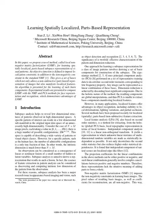
Learning Spatially Localized,Parts-Based Representation Stan Z.Li,XinWen Hou,HongJiang Zhang,QianSheng Cheng.Microsoft Research China,Beijing Sigma Center,Beijing100080,ChinaInstitute of Mathematical Sciences,Peking University,Beijing,ChinaContact:szli@,/szliAbstractIn this paper,we propose a novel method,called local non-negative matrix factorization(LNMF),for learning spa-tially localized,parts-based subspace representation of vi-sual patterns.An objective function is defined to impose lo-calization constraint,in addition to the non-negativity con-straint in the standard NMF[1].This gives a set of bases which not only allows a non-subtractive(part-based)repre-sentation of images but also manifests localized features. An algorithm is presented for the learning of such basis components.Experimental results are presented to compare LNMF with the NMF and PCA methods for face represen-tation and recognition,which demonstrates advantages of LNMF.1IntroductionSubspace analysis helps to reveal low dimensional struc-tures of patterns observed in high dimensional spaces.A specific pattern of interest can reside in a low dimensional sub-manifold in the original input data space of an unnec-essarily high dimensionality.Consider the case ofimage pixels,each taking a value in;there is a huge number of possible configurations:.This space is capable of describing a wide variety of patterns or visual object classes.However,for a specific pattern,such as the human face,the number of admissible configurations is a only tiny fraction of that.In other words,the intrinsic dimension is much lower than.An observation can be considered as a consequence of linear or nonlinear fusion of a small number of hidden or latent variables.Subspace analysis is aimed to derive a rep-resentation that results in such a fusion.In fact,the essence of feature extraction in pattern analysis can be considered as discovering and computing intrinsic low dimension of the pattern from the observation.For these reasons,subspace analysis has been a major research issue in appearance based imaging and vision,such The work presented in the paper was carried out at Microsoft Re-search,China.as object detection and recognition[2,3,4,5,6,7].The significance of is twofold:effective characterization of the pattern and dimension reduction.One approach for learning a subspace representation fora class of image patterns involves deriving a set of basiscomponents for construction of the subspace.The eige-niamge method[2,3,4]uses principal component analy-sis(PCA)[8]performed on a set of representative training data to decorrelate second order moments corresponding to low frequency property.Any image can be represented as a linear combination of these bases.Dimension reduction is achieved by discarding least significant components.Due to the holistic nature of the method,the resulting components are global interpretations,and thus PCA is unable to extract basis components manifesting localized features.However,in many applications,localized features offer advantages in object recognition,including stability to lo-cal deformations,lighting variations,and partial occlusion.Several methods have been proposed recently for localized (spatially),parts-based(non-subtractive)feature extraction.Local feature analysis(LFA)[9],also based on second order statistics,is a method for extracting,from the holis-tic(global)PCA basis,local topographic representation in terms of local features.Independent component analysis [10,11]is a linear non-orthogonal transform.It yields a representation in which unknown linear mixtures of multi-dimensional random variables are made as statistically in-dependent as possible.It not only decorrelates the second order statistics but also reduces higher-order statistical de-pendencies.It is found that independent component of nat-ural scenes are localized edge-likefilters[12].The projection coefficients for the linear combinations in the above methods can be either positive or negative,and such linear combinations generally involve complex cancel-lations between positive and negative numbers.Therefore, these representations lack the intuitive meaning of adding parts to form a whole.Non-negative matrix factorization(NMF)[1]imposes the non-negativity constraints in learning basis images.The pixel values of resulting basis images,as well as coeffi-cients for reconstruction,are all non-negative.This way, 1only non-subtractive combinations are allowed.This en-sures that the components are combined to form a whole in the non-subtractive way.For this reason,NMF is consid-ered as a procedure for learning a parts-based representa-tion[1].However,the additive parts learned by NMF are not necessarily localized,and moreover,we found that the original NMF representation yields low recognition accu-racy,as will be shown.In this paper,we propose a novel subspace method, called local non-negative matrix factorization(LNMF),for learning spatially localized,parts-based representation of visual patterns.Inspired by the original NMF[1],the aim of this work to impose the locality of features in basis com-ponents and to make the representation suitable for tasks where feature localization is important.An objective func-tion is defined to impose the localization constraint,in addi-tion to the non-negativity constraint of[1].A procedure is presented to optimize the objective to learn truly localized, parts-based components.A proof of the convergence of the algorithm is provided.The rest of the paper is organized as follows:Section2 introduces NMF in contrast to PCA.This is followed by the formulation of LNMF.A LNMF learning procedure is presented and its convergence proved.Section3presents experimental results illustrating properties of LNMF and its performance in face recognition as compared to PCA and NMF.2Constrained Non-Negative Matrix FactorizationLet a set of training images be given as an matrix,with each column consisting of the non-negative pixel values of an image.Denote a set of basis images by an matrix.Each image can be represented as a linear combination of the basis images using the approximate factorization(1)where is the matrix of coefficients or weights. Dimension reduction is achieved when.The PCA factorization requires that the basis images (columns of be orthonormal and the rows of be mu-tually orthogonal.It imposes no other constraints than the orthogonality,and hence allows the entries of and to be of arbitrary sign.Many basis images,or eigenfaces in the case of face recognition,lack intuitive meaning,and a linear combination of the bases generally involves complex cancellations between positive and negative numbers.The NMF and LNMF representations allow only positive coef-ficients and thus non-subtractive combinations.2.1NMFNMF imposes the non-negativity constraints instead of the orthogonality.As the consequence,the entries of and are all non-negative,and hence only non-subtractive combi-nations are allowed.This is believed to be compatible to the intuitive notion of combining parts to form a whole,and is how NMF learns a parts-based representation[1].It is alsoconsistent with the physiological fact that thefiring rate are non-negative.NMF uses the divergence of from,defined as(2)as the measure of cost for factorizing into.An NMF factorization is defined as(3)where means that all entries of and are non-negative.reduces to Kullback-Leibler di-vergence when.The above optimization can be done by using multiplicative updaterules[13],for which a matlab program is available at under the“Compu-tational Neuroscience”discussion category.2.2LNMFThe NMF model defined by the constrained minimization of(2)does not impose any constraints on the spatial locality and therefore minimizing the objective function can hardly yield a factorization which reveals local features in the data .Letting,,both being,LNMF is aimed at learning local features by imposing the following three additional constraints on the NMF basis:1.A basis component should not be further decomposedinto more components,so as to minimize the num-ber of basis components required to represent.Letbe a basis vector.Given the existing constraints for all,we wish thatshould be as small as possible so that contains asmany non-zero elements as possible.This can be im-posed by.2.Different bases should be as orthogonal as possible,so as to minimize redundancy between different bases.This can be imposed by.23.Only components giving most important informationshould be retained.Given that every image inhas been normalized into a certain range such as,the total“activity”on each retained com-ponent,defined as the total squared projection coef-ficients summed over all training images,should bemaximized.This is imposed by.The incorporated of the above constraints leads the fol-lowing constrained divergence as the objective function for LNMF:(4)where are some constants.A LNMF factorization is defined as a solution to the constrained minimization of(5).A local solution to the above constrained minimization can be found by using the following three step update rules:(5)(6)(7) 2.3Convergence ProofThe learning algorithm(5)-(7)alternates between updating and updating,which is derived based on a technique in which an objective function is minimized by using an auxiliary function.is said to be an auxiliary function for if andare satisfied.If is an auxiliary function, then is non-increasing when is updated using[14].This is because.Updating:is updated by minimizingwithfixed.An auxiliary function is con-structed for as(8)It is easy to verify.The following proves.Because is a convex function,the following holds for all and:(9)Let(10)Then(11)which is.To minimize w.r.t.,we can update using(12)Such an can be found by letting for all.Because(13)wefind(14)There exists such that(15)where(16)and is a function of and.The result we want to derive from the LNMF learning is the basis,and itself is not so important.Becausewill be normalized by Eq.7,the normalized is regardless of the value as long as.Therefore,we simply replace Eq.(15)by(5).3Updating:is updated by minimizingwithfixed.The auxiliary function foris(17)We can prove andlikewise.By letting,wefind(18)Because and is an approximately orthog-onal basis,and,there must be.Therefore,we can always set the ratio to be not too large(e.g.)so that and thus.Therefore,we have Eq.(6).From the above analysis,we conclude that the three step update rules(5)-(7)results in a sequence of non-increasing values of,and hence converges to a local mini-mum of it.2.4Face Recognition in SubspaceFace recognition in the PCA,NMF or LNMF linear sub-space is performed as follows:1.Feature extraction.Let be the mean of training im-ages.Each training face image is projected into thelinear space as a feature vectorwhich is then used as a prototype feature point.Aquery face image to be classified is represented byits projection into the space as.2.Nearest neighbor classification.The Euclidean dis-tance between the query and each prototype,,is calculated.The query is classified to the class towhich the closest prototype belongs.3Experiments3.1Data PreparationThe Cambridge ORL face database is used for deriving PCA,NMF and LNMF bases.There are400images ()of40persons,10images per person(Fig.1shows the10images of one person).The images are taken at different times,varying lighting slightly,facial expressions (open/closed eyes,smiling/non-smiling)and facial details (glasses/no-glasses).All the images are taken against a dark homogeneous background.The faces are in up-right posi-tion of frontal view,with slight left-right out-of-plane rota-tion.Each image is linearly stretched to the full range of pixel values of[0,255].Figure1:Face examples from ORL database.The set of the10images for each person is randomly partitioned into a training subset of5images and a test set of the other5.The training set is then used to learn basis components,and the test set for evaluate.All the compared methods take the same training and test data.3.2Learning Basis ComponentsLNMF,NMF and PCA representations withbasis components are com-puted from the training set.The matlab package from is used for NMF. NMF converges about5-times faster than LNMF.Fig.2 shows the resulting LNMF and NMF components for subspaces of dimensions25,49and81.Higher pixel values are in in darker color;the components in each LNMF basis set have been ordered(left-right then top-down) according to the significance value.The NMF bases are as holistic as the PCA basis(eigenfaces)for the training set.We notice the result presented in[1]does not appear so,perhaps because the faces used for producing that result are well aligned.The LNMF procedure learns basis components which not only lead to non-subtractive representations,but also manifest localized features and thus truly parts-based representations.Also,we see that as the dimension(number of components)increases,the features formed in the LNMF components become more localized.4Figure2:LNMF(left)and NMF(right)bases of dimen-sions25(row1),49(row2)and81(row3).Every basis component is of size and the displayed images are re-sized tofit the paper format.The LNMF representation is both parts-based and local,whereas NMF is parts-based but holistic.3.3ReconstructionFig.3shows reconstructions in the LNMF,NMF and PCA subspaces of various dimensions for a face image in the test set which corresponds to the one in the middle of row1 of Fig.1.As the dimension is increased,more details are recovered.We see that while NMF and PCA reconstruc-tions look similar in terms of the smoothness and texture of the reconstructed images,with PCA presenting better reconstruction quality than NMF.Surprisingly the LNMF representation,which is based on more localized features, provides smoother reconstructions than NMF and PCA. 3.4Face RecognitionThe LNMF,NMF and PCA representations are compara-tively evaluated for face recognition using the images from the test set.The recognition accuracy,defined as the per-centage of correctly recognized faces,is used as the per-formance measure.Tests are done with varying numberofFigure3:Reconstructions of the face image in the(left to right)25,49,81and121dimensional(top-down)LNMF, NMF,and PCAsubspaces.Figure4:Examples of random occluding patches of sizes (from left to right)10x10,20x20,...,50x50,60x60.basis components,with or without occlusion.The occlu-sion is simulated in an image by using a white patch of size with at a random location;see Fig.4for examples.Figs.5and6show recognition accuracy curves under various conditions.Fig.5compares the three representa-tions in terms of the recognition accuracies versus the num-ber of basis components for.The LNMF yields the best recognition accuracy,slightly better than PCA whereas the original NMF gives very low accuracy.Fig.6compares the three representations un-der varying degrees of occlusion and with varying num-ber of basis components,in terms of the recognition ac-curacies versus the size of occluding patch for.As we see,although PCA yields more favorable results than LNMF when the patch size is small, the better stability of the LNMF representation under partial occlusion becomes clear as the patch size increases.4ConclusionIn this paper,we have proposed a new method,local non-negative matrix factorization(LNMF),for learning spatially5Figure5:Recognition accuracies as function of the num-ber(in5x5,6x6,...,11x11)of basis components used,for the LNMF(solid)and NMF(dashed)and PCA(dot-dashed) representations.Figure6:Recognition accuracies versus the size(in10x10, 20x20,...,60x60)of occluding patches,with25,49,81,121 basis components(left-right,then top-down),for the LNMF (solid)and NMF(dashed)and PCA(dot-dashed)represen-tations.localized,part-based subspace representation of visual pat-terns.The work is aimed to learn localized of features in NMF basis components suitable for tasks such as face recognition.An algorithms is presented for the learning and its convergence proved.Experimental results have shown that we have achieved our objectives:LNMF derives bases which are better suited for a localized representation than PCA and NMF,and leads to better recognition results than the existing methods.The LNMF and NMF learning algorithms are local min-imizers.They give different basis components from differ-ent initial conditions.We will investigate how this affects the recognition rate.Further future work includes the fol-lowing topics.Thefirst is to develop algorithms for faster convergence and better solution in terms of minimizing theobjective function.The second is to investigate the abil-ity of the model to generalize,i.e.how the constraints,the non-negativity and others,are satisfied for data not seen in the training set.The third is to compare with other methods for learning spatially localized features such as LFA[9]and ICA[12].References[1] D.D.Lee and H.S.Seung,““Learning the parts of objectsby non-negative matrix factorization”,”Nature,vol.401,pp.788–791,1999.[2]L.Sirovich and M.Kirby,““Low-dimensional procedurefor the characterization of human faces”,”Journal of theOptical Society of America A,vol.4,no.3,pp.519–524,March1987.[3]M.Kirby and L.Sirovich,““Application of the Karhunen-Loeve procedure for the characterization of human faces”,”IEEE Transactions on Pattern Analysis and Machine Intelli-gence,vol.12,no.1,pp.103–108,January1990.[4]Matthew A.Turk and Alex P.Pentland,““Face recognitionusing eigenfaces.”,”in Proceedings of IEEE Computer Soci-ety Conference on Computer Vision and Pattern Recognition,Hawaii,June1991,pp.586–591.[5]David Beymer,Amnon Shashua,and Tomaso Poggio,““Ex-ample based image analysis and synthesis”,” A.I.Memo1431,MIT,1993.[6] A.P.Pentland,B.Moghaddam,and T.Starner,““View-based and modular eigenspaces for face recognition”,”inProceedings of IEEE Computer Society Conference on Com-puter Vision and Pattern Recognition,1994,pp.84–91.[7]H.Murase and S.K.Nayar,““Visual learning and recogni-tion of3-D objects from appearance”,”International Journalof Computer Vision,vol.14,pp.5–24,1995.[8]K.Fukunaga,Introduction to statistical pattern recognition,Academic Press,Boston,2edition,1990.[9]P.Penev and J.Atick,““Local feature analysis:A generalstatistical theory for object representation”,”Neural Systems,vol.7,no.3,pp.477–500,1996.[10] C.Jutten and J.Herault,““Blind separation of sources,partI:An adaptive algorithm based on neuromimetic architec-ture”,”Signal Processing,vol.24,pp.1–10,1991.[11]on,““Independent component analysis-a new con-cept?”,”Signal Processing,vol.36,pp.287–314,1994.[12] A.J.Bell and T.J.Sejnowski,““The‘independent compo-nents’of natural scenes are edgefilters”,”Vision Research,vol.37,pp.3327–3338,1997.[13] D.D.Lee and H.S.Seung,““Algorithms for non-negativematrix factorization”,”in Proceedings of Neural InformationProcessing Systems,2000.[14] A.P.Dempster,ird,and D.B.Bubin,““Maxi-mum likelihood from imcomplete data via EM algorithm”,”Journal of the Royal Statistical Society,Series B,vol.39,pp.1–38,1977.6。

explanatory factors for the observed input. A good representation is also one that is useful as input to a supervised predictor. Among the various ways of learning representations, this paper focuses on deep learning methods: those that are formed by the composition of multiple non-linear transformations, with the goal of yielding more abstract – and ultimately more useful – representations. Here we survey this rapidly developing area with special emphasis on recent progress. We consider some of the fundamental questions that have been driving research in this area. Specifically, what makes one representation better than another? Given an example, how should we compute its representation, i.e. perform feature extraction? Also, what are appropriate objectives for learning good representations?

读书的方法英语作文Title: Effective Methods for Effective Reading。

Reading is an essential skill that contributes significantly to one's intellectual growth and academic success. However, mastering the art of reading requires more than just going through the motions. It involves employing effective methods and strategies to comprehend, analyze, and retain information. In this essay, we will explore various techniques for enhancing reading skills.1. Active Reading: Active reading involves engaging with the text actively rather than passively absorbing information. This can be achieved through techniques such as highlighting key points, taking notes, and asking questions while reading. By actively interacting with the material, readers can better comprehend and remember the content.2. Skimming and Scanning: Skimming and scanning areuseful techniques for quickly locating specific information within a text. Skimming involves rapidly reading through the text to get a general idea of its content, while scanning involves looking for particular keywords or phrases. These techniques are particularly helpful when trying to locate specific information within lengthy texts or documents.3. Previewing: Before diving into a text, it can be beneficial to preview it by examining the title, headings, subheadings, and any visual aids such as graphs or illustrations. Previewing provides readers with a roadmap of the text's structure and main ideas, making it easier to understand the material as they read.4. Chunking: Chunking involves breaking down large pieces of information into smaller, more manageable chunks. This can be done by dividing the text into sections or paragraphs and focusing on one chunk at a time. By breaking the material into smaller parts, readers can better digest and comprehend the information.5. Summarizing: Summarizing involves distilling themain ideas and key points of a text into concise summaries. This can be done either during or after reading and helps reinforce understanding by requiring readers to process and synthesize the information in their own words. Summarizingis an effective way to reinforce learning and retention.6. Visualization: Visualization involves creatingmental images or representations of the material being read. This can help readers better understand abstract conceptsor complex information by making it more concrete and tangible. Visualization can be particularly useful when reading descriptive or narrative texts.7. Active Recall: Active recall involves actively retrieving information from memory rather than simply re-reading the text. This can be done through techniques such as self-quizzing or summarizing the material without referring back to the text. Active recall strengthens memory and comprehension by forcing readers to actively engage with the material.8. Reviewing: Reviewing involves periodicallyrevisiting and reviewing previously read material to reinforce learning and retention. This can be done through techniques such as spaced repetition, where material is revisited at increasing intervals over time. Reviewing is essential for long-term retention and mastery of the material.In conclusion, effective reading requires the application of various techniques and strategies to comprehend, analyze, and retain information. By incorporating active reading, skimming and scanning, previewing, chunking, summarizing, visualization, active recall, and reviewing into their reading routine, readers can enhance their reading skills and achieve greater success in their academic and professional endeavors.。

高一人工智能英语阅读理解25题1<背景文章>Artificial intelligence (AI) has become one of the most talked - about topics in recent years. AI can be defined as the simulation of human intelligence processes by machines, especially computer systems. These processes include learning, reasoning, problem - solving, perception, and language understanding.The development of AI has a long history. It started in the 1950s when the concept was first introduced. In the early days, AI research focused on simple tasks like playing games and solving basic mathematical problems. However, with the development of computer technology and the increase in data availability, AI has made great strides.AI has found applications in various fields. In the medical field, AI can assist doctors in diagnosing diseases. For example, it can analyze medical images such as X - rays and MRIs to detect early signs of diseases that might be missed by human eyes. In education, AI - powered tutoring systems can provide personalized learning experiences for students. They can adapt to the individual learning pace and style of each student, helping them to better understand difficult concepts. In the transportation industry, self - driving cars, which are a significant application of AI, are expectedto revolutionize the way we travel. They can potentially reduce traffic accidents caused by human error and improve traffic efficiency.However, AI also brings some potential negative impacts. One concern is the impact on employment. As AI systems can perform many tasks that were previously done by humans, there is a fear that many jobs will be lost. For example, jobs in manufacturing, customer service, and some administrative tasks may be at risk. Another issue is the ethical considerations. For instance, how should AI make decisions in life - or - death situations? And there are also concerns about data privacy as AI systems rely on large amounts of data.1. <问题1>What is the main idea of this passage?A. To introduce the development of computer technology.B. To discuss the applications and impacts of artificial intelligence.C. To explain how to solve problems in different fields.D. To show the importance of data in AI systems.答案：B。

基于AHK中德职教项目构建“六步三环”学习模式的实践探索*孙跃岗，陈世鹏，陈紫晗（集美工业学校，福建厦门 361022）【摘要】汲取学习德国双元制课程体系的优势，将德国职业标准和职业资格认证内容引入教学实际中，将课程体系进行本地化的改造提升。

以专业核心课程《机电设备安装与调试》为例进行实践探索，以项目为载体、任务为驱动、工作过程为导向开展教学研究，构建行动领域课程体系；依托“六步三环”组织教学，培养新时代融合性技术人才，服务本地高端制造产业。

关键词：行动领域；AHK；三教改革中图分类号：G712 文献标识码：BDOI：10.13596/ki.44-1542/th.2024.03.032Practical Exploration of Constructing a "Six Steps Three Rings"Learning Model Based on AHK Sino GermanVocational Education ProjectSun Yuegang，Chen Shipeng，Chen Zihan（Jimei Industrial School, Xiamen, Fujian 361022, CHN）【Abstract】Drawing on the advantages of the German dual curriculum system, the German voca⁃tional standards and vocational qualification certification are introduced into the teaching practice, and the curriculum system is "localized" to transform and upgrade. The author takes the profes⁃sional core course "Mechanical and Electrical Equipment Installation and Commissioning" as an ex⁃ample for practical exploration, and carries out teaching and research with the project as the carrier, the task as the driver, and the work process as the guidance, and constructs the curriculum system in the field of action. Relying on the "six steps and three rings" to organize teaching, cultivate in⁃tegrated technical talents in the new era, and serve the local high-end manufacturing industry. Key words:areas of action；AHK；three education reform1引言我国从20世纪80年代就开始考察学习德国职业教育，在多年的探索和实践中，真正的德国双元制并没有在国内遍地开花结果。

第47卷第1期Vol.47No.1计算机工程Computer Engineering2021年1月January2021一种融合主题特征的自适应知识表示方法陈文杰（中国科学院成都文献情报中心，成都610041）摘要：基于翻译的表示学习模型TransE被提出后,研究者提出一系列模型对其进行改进和补充,如TransH、TransG、TransR等。

然而,这类模型往往孤立学习三元组信息,忽略了实体和关系相关的描述文本和类别信息。

基于主题特征构建TransATopic模型,在学习三元组的同时融合关系中的描述文本信息,以增强知识图谱的表示效果。

采用基于主题模型和变分自编器的关系向量构建方法,根据关系上的主题分布信息将同一关系表示为不同的实值向量,同时将损失函数中的距离度量由欧式距离改进为马氏距离,从而实现向量不同维权重的自适应赋值。

实验结果表明,在应用于链路预测和三元组分类等任务时,TransATopic模型的MeanRank、HITS@5和HITS@10指标较TransE模型均有显著改进。

关键词：知识图谱；表示学习；主题模型；变分自编码器；马氏距离开放科学（资源服务）标志码（OSID）：中文引用格式：陈文杰.一种融合主题特征的自适应知识表示方法［J］.计算机工程，2021，47（1）：87-93，100.英文引用格式：CHEN Wenjie.An adaptive approach for knowledge representation fused with topic feature［J］.Computer Engineering，2021，47（1）：87-93，100.An Adaptive Approach for Knowledge Representation Fused with Topic FeatureCHEN Wenjie（Chengdu Library and Information Center，Chinese Academy of Science，Chengdu610041，China）【Abstract】Since the emergence of the translation-based representation learning model，TransE，a series of models such as TransH，TransG and TransR have been proposed to improve and add functions to TransE.However，such models tend to learn triplet information in isolation，and ignore the descriptive text and category information related to entities and relations.Therefore，this paper fuses descriptive text information of relations while learning triples，and constructs the TransATopic model based on topic features to enhance the representation effect of the knowledge graph.The relation vector construction method based on the topic model and Variational Autoencoder（VAE）is used to map one relation to different real-valued vectors according to topic distribution information of relations.At the same time，the distance metric in the loss function is improved from Euclidean distance to a more flexible Mahalanobis distance，which realizes the adaptive assignment of vector weights in different dimensions.Experimental results show that when applied to link prediction and triple classification tasks，TransATopic’s indicators including MeanRank，HITS@5and HITS@10are significantly improved compared with the TransE model.【Key words】knowledge graph；representation learning；topic model；Variational Autoencoder（VAE）；Mahalanobis distanceDOI：10.19678/j.issn.1000-3428.00566880概述知识图谱是由三元组构成的结构化语义知识库，其以符号的形式描述现实世界中实体和实体间的连接关系。

shapelet-based representation learning -回复什么是shapeletbased representation learning? 这个方法如何运作? 其有哪些应用领域? 推文。

Shapeletbased representation learning 是一种基于形状片段的表示学习方法。

它通过在时间序列数据中发现具有显著形状特征的片段，然后将每个片段分为两个类别，即形状片段和非形状片段，以实现对时间序列数据的有意义表示。

本文将逐步解释此方法的运作原理，并探讨其在不同领域的应用。

首先，shapeletbased representation learning 方法使用形状片段作为原始时间序列数据的表示。

形状片段是对时间序列数据中重要特征的局部描述。

这些片段通常是具有显著特征的子序列，例如在连续的时间序列数据中具有一定幅度的波形变化或突发事件。

通过找到这些形状片段，我们可以将时间序列数据转换为更简洁且具有意义的表示。

为了发现形状片段，shapeletbased representation learning 方法通常使用子序列匹配技术。

在此过程中，方法将时间序列数据划分为多个子序列，并计算每个子序列与原始时间序列数据之间的相似度得分。

相似度得分可以通过计算两个时间序列之间的距离来确定，例如欧氏距离或动态时间规整。

然后，通过寻找具有高相似度得分的子序列，方法可以发现具有显著特征的形状片段。

找到形状片段后，shapeletbased representation learning 方法将它们划分为两个类别：形状片段和非形状片段。

形状片段是指对时间序列数据的重要特征有显著影响的片段。

非形状片段则是指不具有显著特征的片段。

这种分离可以通过训练一个机器学习模型来实现，例如支持向量机（SVM）或神经网络。

模型可以使用形状片段和非形状片段作为训练样本，通过学习它们之间的区别和类别特征，来进行时间序列数据的表示学习。

Nonnegative Matrix Factorization:A Comprehensive ReviewYu-Xiong Wang,Student Member,IEEE,and Yu-Jin Zhang,Senior Member,IEEE Abstract—Nonnegative Matrix Factorization(NMF),a relatively novel paradigm for dimensionality reduction,has been in the ascendant since its inception.It incorporates the nonnegativity constraint and thus obtains the parts-based representation as well as enhancing the interpretability of the issue correspondingly.This survey paper mainly focuses on the theoretical research into NMF over the last5years,where the principles,basic models,properties,and algorithms of NMF along with its various modifications,extensions, and generalizations are summarized systematically.The existing NMF algorithms are divided into four categories:Basic NMF(BNMF), Constrained NMF(CNMF),Structured NMF(SNMF),and Generalized NMF(GNMF),upon which the design principles,characteristics,problems,relationships,and evolution of these algorithms are presented and analyzed comprehensively.Some related work not on NMF that NMF should learn from or has connections with is involved too.Moreover,some open issues remained to be solved are discussed.Several relevant application areas of NMF are also briefly described.This survey aims to construct an integrated,state-of-the-art framework for NMF concept,from which the follow-up research may benefit.Index Terms—Data mining,dimensionality reduction,multivariate data analysis,nonnegative matrix factorization(NMF)Ç1I NTRODUCTIONO NE of the basic concepts deeply rooted in science and engineering is that there must be something simple, compact,and elegant playing the fundamental roles under the apparent chaos and complexity.This is also the case in signal processing,data analysis,data mining,pattern recognition,and machine learning.With the increasing quantities of available raw data due to the development in sensor and computer technology,how to obtain such an effective way of representation by appropriate dimension-ality reduction technique has become important,necessary, and challenging in multivariate data analysis.Generally speaking,two basic properties are supposed to be satisfied: first,the dimension of the original data should be reduced; second,the principal components,hidden concepts,promi-nent features,or latent variables of the data,depending on the application context,should be identified efficaciously.In many cases,the primitive data sets or observations are organized as data matrices(or tensors),and described by linear(or multilinear)combination models;whereupon the formulation of dimensionality reduction can be regarded as, from the algebraic perspective,decomposing the original data matrix into two factor matrices.The canonical methods, such as Principal Component Analysis(PCA),Linear Discriminant Analysis(LDA),Independent Component Analysis(ICA),Vector Quantization(VQ),etc.,are the exemplars of such low-rank approximations.They differ from one another in the statistical properties attributable to the different constraints imposed on the component matrices and their underlying structures;however,they have something in common that there is no constraint in the sign of the elements in the factorized matrices.In other words,the negative component or the subtractive combina-tion is allowed in the representation.By contrast,a new paradigm of factorization—Nonnegative Matrix Factoriza-tion(NMF),which incorporates the nonnegativity constraint and thus obtains the parts-based representation as well as enhancing the interpretability of the issue correspondingly, was initiated by Paatero and Tapper[1],[2]together with Lee and Seung[3],[4].As a matter of fact,the notion of NMF has a long history under the name“self modeling curve resolution”in chemometrics,where the vectors are continuous curves rather than discrete vectors[5].NMF was first introduced by Paatero and Tapper as the concept of Positive Matrix Factorization,which concentrated on a specific application with Byzantine algorithms.These shortcomings limit both the theoretical analysis,such as the convergence of the algorithms or the properties of the solutions,and the generalization of the algorithms in other applications. Fortunately,NMF was popularized by Lee and Seung due to their contributing work of a simple yet effective algorithmic procedure,and more importantly the emphasis on its potential value of parts-based representation.Far beyond a mathematical exploration,the philosophy underlying NMF,which tries to formulate a feasible model for learning object parts,is closely relevant to perception mechanism.While the parts-based representation seems intuitive,it is indeed on the basis of physiological and psychological evidence:perception of the whole is based on perception of its parts[6],one of the core concepts in certain computational theories of recognition problems.In fact there are two complementary connotations in nonnegativity—nonnegative component and purely additive combination. On the one hand,the negative values of both observations.The authors are with the Tsinghua National Laboratory for InformationScience and Technology and the Department of Electronic Engineering,Tsinghua University,Rohm Building,Beijing100084,China.E-mail:albertwyx@,zhang-yj@.Manuscript received21July2011;revised2Nov.2011;accepted4Feb.2012;published online2Mar.2012.Recommended for acceptance by L.Chen.For information on obtaining reprints of this article,please send e-mail to:tkde@,and reference IEEECS Log Number TKDE-2011-07-0429.Digital Object Identifier no.10.1109/TKDE.2012.51.1041-4347/13/$31.00ß2013IEEE Published by the IEEE Computer Societyand latent components are physically meaningless in many kinds of real-world data,such as image,spectra,and gene data,analysis tasks.Meanwhile,the discovered prototypes commonly correspond with certain semantic interpretation. For instance,in face recognition,the learned basis images are localized rather than holistic,resembling parts of faces,such as eyes,nose,mouth,and cheeks[3].On the other hand, objects of interest are most naturally characterized by the inventory of its parts,and the exclusively additive combina-tion means that they can be reassembled by adding required parts together similar to identikits.NMF thereupon has achieved great success in real-word scenarios and tasks.In document clustering,NMF surpasses the classic methods, such as spectral clustering,not only in accuracy improve-ment but also in latent semantic topic identification[7].To boot,the nonnegativity constraint will lead to sort of sparseness naturally[3],which is proved to be a highly effective representation distinguished from both the com-pletely distributed and the solely active component de-scription[8].When NMF is interpreted as a neural network learning algorithm depicting how the visible variables are generated from the hidden ones,the parts-based represen-tation is obtained from the additive model.A positive number indicates the presence and a zero value represents the absence of some event or component.This conforms nicely to the dualistic properties of neural activity and synaptic strengths in neurophysiology:either excitatory or inhibitory without changing sign[3].Because of the enhanced semantic interpretability under the nonnegativity and the ensuing sparsity,NMF has become an imperative tool in multivariate data analysis, and been widely used in the fields of mathematics, optimization,neural computing,pattern recognition and machine learning[9],data mining[10],signal processing [11],image engineering and computer vision[11],spectral data analysis[12],bioinformatics[13],chemometrics[1], geophysics[14],finance and economics[15].More specifi-cally,such applications include text data mining[16],digital watermark,image denoising[17],image restoration,image segmentation[18],image fusion,image classification[19], image retrieval,face hallucination,face recognition[20], facial expression recognition[21],audio pattern separation [22],music genre classification[23],speech recognition, microarray analysis,blind source separation[24],spectro-scopy[25],gene expression classification[26],cell analysis, EEG signal processing[17],pathologic diagnosis,email surveillance[10],online discussion participation prediction, network security,automatic personalized summarization, identification of compounds in atmosphere analysis[14], earthquake prediction,stock market pricing[15],and so on.There have been numerous results devoted to NMF research since its inception.Researchers from various fields, mathematicians,statisticians,computer scientists,biolo-gists,and neuroscientists,have explored the NMF concept from diverse perspectives.So a systematic survey is of necessity and consequence.Although there have been such survey papers as[27],[28],[12],[13],[10],[11],[29]and one book[9],they fail to reflect either the updated or the comprehensive results.This review paper will summarize the principles,basic models,properties,and algorithms of NMF systematically over the last5years,including its various modifications,extensions,and generalizations.A taxonomy is accordingly proposed to logically group them, which have not been presented before.Besides these,some related work not on NMF that NMF should learn from or has connections with will also be involved.Furthermore, this survey mainly focuses on the theoretical research rather than the specific applications,the practical usage will also be concerned though.It aims to construct an integrated, state-of-the-art framework for NMF concept,from which the follow-up research may benefit.In conclusion,the theory of NMF has advanced sig-nificantly by now yet is still a work in progress.To be specific:1)the properties of NMF itself have been explored more deeply;whereas a firm statistical underpinning like those of the traditional factorization methods—PCA or LDA—is not developed fully(partly due to its knottiness).2)Some problems like the ones mentioned in[29]have been solved,especially those with additional constraints;never-theless a lot of other questions are still left open.The existing NMF algorithms are divided into four categories here given in Fig.1,following some unified criteria:1.Basic NMF(BNMF),which only imposes the non-negativity constraint.2.Constrained NMF(CNMF),which imposes someadditional constraints as regularization.3.Structured NMF(SNMF),which modifies the stan-dard factorization formulations.4.Generalized NMF(GNMF),which breaks throughthe conventional data types or factorization modesin a broad sense.The model level from Basic to Generalized NMF becomes broader.Therein Basic NMF formulates the fundamental analytical framework upon which all other NMF models are built.We will present the optimization tools and computational methods to efficiently and robustly solve Basic NMF.Moreover,the pragmatic issue of NMF with respect to large-scale data sets and online processing will also be discussed.Constrained NMF is categorized into four subclasses:1.Sparse NMF(SPNMF),which imposes the sparse-ness constraint.2.Orthogonal NMF(ONMF),which imposes theorthogonality constraint.3.Discriminant NMF(DNMF),which involves theinformation for classification and discrimination.4.NMF on manifold(MNMF),which preserves thelocal topological properties.We will demonstrate why these morphological constraints are essentially necessary and how to incorporate them into the existing solution framework of Basic NMF.Correspondingly,Structured NMF is categorized into three subclasses:1.Weighed NMF(WNMF),which attaches differentweights to different elements regarding their relativeimportance.2.Convolutive NMF (CVNMF),which considers the time-frequency domain factorization.3.Nonnegative Matrix Trifactorization (NMTF),whichdecomposes the data matrix into three factor matrices.Besides,Generalized NMF is categorized into four subclasses:1.Semi-NMF,which relaxes the nonnegativity con-straint only on the specific factor matrix.2.Nonnegative Tensor Factorization (NTF),whichgeneralizes the matrix-form data to higher dimen-sional tensors.3.Nonnegative Matrix-Set Factorization (NMSF),which extends the data sets from matrices to matrix-sets.4.Kernel NMF (KNMF),which is the nonlinear modelof NMF.The remainder of this paper is organized as follows:first,the mathematic formulation of NMF model is presented,and the unearthed properties of NMF are summarized.Then the algorithmic details of foregoing categories of NMF are elaborated.Finally,conclusions are drawn,and some open issues remained to be solved are discussed.2C ONCEPT AND P ROPERTIES OF NMFDefinition.Given an M dimensional random vector x with nonnegative elements,whose N observations are denoted asx j;j ¼1;2;...;N ,let data matrix be X ¼½x 1;x 2;...;x N 2I R M ÂN!0,NMF seeks to decompose X into nonnegative M ÂL basismatrix U ¼½u 1;u 2;...;u L 2I R M ÂL!0and nonnegative L ÂN coefficient matrix V ¼½v 1;v 2;...;v N 2I R L ÂN!0,such thatX %U V ,where I R M ÂN!0stands for the set of M ÂN element-wise nonnegative matrices.This can also be written as the equivalent vector formula x j %P Li ¼1u i V ij .It is obvious that v j is the weight coefficient of the observation x j on the columns of U ,the basis vectors or the latent feature vectors of X .Hence,NMF decomposes each data into the linear combination of the basis vectors.Because of the initial condition L (min ðM;N Þ,the obtained basis vectors are incomplete over the original vector space.In other words,this approach tries to represent the high-dimensional stochastic pattern with far fewer bases,so the perfect approximation can be achieved successfully only if the intrinsic features are identified in U .Here,we discuss the relationship between L and M ,N a little more.In most cases,NMF is viewed as a dimension-ality reduction and feature extraction technique with L (M;L (N ;that is,the basis set learned from NMF model is incomplete,and the energy is compacted.However,in general,L can be smaller,equal or larger than M .But there are fundamental differences in the decomposition for L <M and L >M .It is a sort of sparse coding and compressed sensing with overcomplete basis when L >M .Hence,L need not be limited by the dimensionality of the data,which is useful for some applications,like classification.In this situation,it may benefit from the sparseness due to both nonnegativity and redundant representation.One approach to obtain this NMF model is to perform the decomposition on the residue matrix E ¼X ÀU V repeat-edly and sequentially [30].As a kind of matrix factorization model,three essential questions need answering:1)existence,whether the nontrivial NMF solutions exist;2)uniqueness,under what assumptions NMF is,at least in some sense,unique;3)effectiveness,under what assumptions NMF is able to recover the “right answer.”The existence was showed via the theory of Completely Positive (CP)Factorization for the first time in [31].The last two concerns were first mentioned and discussed from a geometric viewpoint in [32].Complete NMF X ¼U V is considered first for the analysis of existence,convexity,and computational com-plexity.The trivial solution always exists as U ¼X and V ¼I N .By relating NMF to CP Factorization,Vasiloglou et al.showed that every nonnegative matrix has a nontrivial complete NMF [31].As such,CP Factorizationis a special case,where a nonnegative matrix X 2I R M ÂM!0is CP if it can be factored in the form X ¼U U T ;U 2I R M ÂL!0.The minimum L is called the CP-rank of X .WhenFig.1.The categorization of NMF models and algorithms.combining that the set of CP matrices forms a convex cone with that the solution to NMF belongs to a CP cone, solving NMF is a convex optimization problem[31]. Nevertheless,finding a practical description of the CP cone is still open,and it remains hard to formulate NMF as a convex optimization problem,despite a convex relaxation to rank reduction with theoretical merit pro-posed in[31].Using the bilinear model,complete NMF can be rewritten as linear combination of rank-one nonnegative matrices expressed byX¼X Li¼1U i V i ¼X Li¼1U i V iðÞT;ð1Þwhere U i is the i th column vector of U while V i is the i th row vector of V,and denotes the outer product of two vectors.The smallest L making the decomposition possible is called the nonnegative rank of the nonnegative matrix X, denoted as rankþðXÞ.And it satisfies the following trivial bounds[33]rankðXÞrankþðXÞminðM;NÞ:ð2ÞWhile PCA can be solved in polynomial time,the optimization problem of NMF,with respect to determining the nonnegative rank and computing the associated factor-ization,is more difficult than its unconstrained counterpart. It is in fact NP-hard when requiring both the dimension and the factorization rank of X to increase,which was proved via relating it to NP-hard intermediate simplex problem by Vavasis[34].This is also the corollary of CP programming, since the CP cone cannot be described in polynomial time despite its convexity.In the special case when rankðXÞ¼1, complete NMF can be solved in polynomial time.However, the complexity of complete NMF for fixed factorization rank generally is still unknown[35].Another related work is so-called Nonnegative Rank Factorization(NRF)focusing on the situation of rankðXÞ¼rankþðXÞ,i.e.,selecting rankðXÞas the minimum L[33]. This is not always possible,and only nonnegative matrix with a corresponding simplicial cone(A polyhedral cone is simplicial if its vertex rays are linearly independent.) existed has an NRF[36].In most cases,the approximation version of NMF X% U V instead of the complete factorization is widely utilized. An alternative generative model isX¼U VþE;ð3Þwhere E2I R MÂN is the residue or noise matrix represent-ing the approximation error.These two modes of NMF are essentially coupled with each other,though much more attention is devoted to the latter.The theoretical results on complete NMF will be helpful to design more efficient NMF algorithms[31],[34]. The selection of the factorization rank L of NMF may be more creditable if tighter bound for the nonnegative rank is obtained[37].In essence,NMF is an ill-posed problem with nonunique solutions[32],[38].From the geometric perspective,NMF can be viewed as finding a simplicial cone involving all the data points in the positive orthant.Given a simplicial cone satisfying all these conditions,it is not difficult to construct another cone containing the former one to meet the same conditions,so the nesting can work on infinitively thus leading to an ill-defined factorization notion.From the algebraic perspective,if there exists a solution X%U0V0, let U¼U0D,V¼DÀ1V0,then X%U V.If a nonsingular matrix and its inverse are both nonnegative,then the matrix is a generalized permutation with the form of P S, where P and S are permutation and scaling matrices, respectively.So the permutation and scaling ambiguities for NMF are inevitable.For that matter,NMF is called unique factorization up to a permutation and a scaling transformation when D¼P S.Unfortunately,there are many ways to select a rotational matrix D which is not necessarily a generalized permutation or even nonnegative matrix,so that the transformed factor matrices U and V are still nonnegative.In other words,the sole nonnegativity constraint in itself will not suffice to guarantee the uniqueness,let alone the effectiveness.Nevertheless,the uniqueness will be achieved if the original data satisfy certain generative model.Intuitively,if U0and V0are sufficiently sparse,only generalized permutation matrices are possible rotation matrices satisfying the nonnegativity constraint.Strictly speaking,this is called boundary close condition for sufficiency and necessity of the uniqueness of NMF solution[39].The deep discussions about this issue can be found in[32],[38],[39],[40],[41],and[42].In practice,incorporating additional constraints such as sparseness in the factor matrices or normalizing the columns of U(respectively rows of V)to unit length is helpful in alleviating the rotational indeterminacy[9].It was hoped that NMF would produce an intrinsically parts-based and sparse representation in unsupervised mode[3],which is the most inspiring benefit of NMF. Intuitively,this can be explained by that the stationary points of NMF solutions will typically be located at the boundary of the feasible domain due to the first order optimality conditions,leading to zero elements[37].Further experiments by Li et al.have shown,however,that the pure additivity does not necessarily mean sparsity and that NMF will not necessarily learn the localized features[43].Further more,NMF is equivalent to k-means clustering when using Square of Euclidian Distance(SED)[44],[45], while tantamount to Probabilistic Latent Semantic Analy-sis(PLSA)when using Generalized Kullback-Leibler Divergence(GKLD)as the objective function[46],[47].So far we may conclude that the merits of NMF,parts-based representation and sparseness included,come at the price of more complexity.Besides,SVD or PCA has always a more compact spectrum than NMF[31].You just cannot have the best of both worlds.3B ASIC NMF A LGORITHMSThe cynosure in Basic NMF is trying to find more efficient and effective solutions to NMF problem under the sole nonnegativity constraint,which lays the foundation for the practicability of NMF.Due to its NP-hardness and lack of appropriate convex formulations,the nonconvex formula-tions with relatively easy solvability are generally adopted,and only local minima are achievable in a reasonable computational time.Hence,the classic and also more practical approach is to perform alternating minimization of a suitable cost function as the similarity measures between X and the product U V .The different optimization models vary from one another mainly in the object functions and the optimization procedures.These optimization models,even serving to give sight of some possible directions for the solutions to Constrained,Structured,and Generalized NMF,are the kernel discus-sions of this section.We will first summarize the objective functions.Then the details about the classic Basic NMF framework and the paragon algorithms are presented.Moreover,some new vision of NMF,such as the geometric formulation of NMF,and the pragmatic issue of NMF,such as large-scale data sets,online processing,parallel comput-ing,and incremental NMF,will be discussed.In the last part of this section,some other relevant issues are also involved.3.1Similarity Measures or Objective FunctionsIn order to quantify the difference between the original data X and the approximation U V ,a similarity measure D ðX U V k Þneeds to be defined first.This is also the objective function of the optimization model.These similarity mea-sures can be either distances or divergences,and correspond-ing objective functions can be either a sole cost function or optionally a set of cost functions with the same global minima to be minimized sequentially or simultaneously.The most commonly used objective functions are SED (i.e.,Frobenius norm)(4)and GKLD (i.e.,I-divergence)(5)[4]D F X U V k ðÞ¼12X ÀU V k k 2F ¼12X ijX ij ÀU V ½ ij 2;ð4ÞD KL X U V k ðÞ¼XijX ij lnX ijU V ½ ijÀX ij þU V ½ ij !:ð5ÞThere are some drawbacks of GKLD,especially the gradients needed in optimization heavily depend on the scales of factorizing matrices leading to many iterations.Thus,the original KLD is renewed for NMF by normalizing the input data in [48].Other cost functions consist of Minkowski family of metrics known as ‘p -norm,Earth Mover’s distance metric [18], -divergence [17], -divergence [49], -divergence [50],Csisza´r’s ’-divergence [51],Bregman divergence [52],and - -divergence [53].Most of them are element-wise mea-sures.Some similarity measures are more robust with respect to noise and outliers,such as hypersurface cost function [54], -divergence [50],and - -divergence [53].Statistically,different similarity measures can be deter-mined based on a prior knowledge about the probability distribution of the noise,which actually reflects the statistical structure of the signals and the disclosed compo-nents.For example,the SED minimization can be seen as a maximum likelihood estimator where the difference is due to additive Gaussian noise,whereas GKLD can be shown to be equivalent to the Expectation Maximization (EM)algo-rithm and maximum likelihood for Poisson processes [9].Given that while the optimization problem is not jointly convex in both U and V ,it is separately convex in either Uor V ,the alternating minimizations are seemly the feasible direction.A phenomenon worthy of notice is that although the generative model of NMF is linear,the inference computation is nonlinear.3.2Classic Basic NMF Optimization Framework The prototypical multiplicative update rules originated by Lee and Seung—the SED-MU and GKLD-MU [4]have still been widely used as the baseline.The SED-MU and GKLD-MU algorithms use SED and GKLD as objective functions,respectively,and both apply iterative multiplicative updates as the optimization approach similar to EM algorithms.In essence,they can be viewed as adaptive rescaled gradient descent algorithms.Considering the efficiency,they are relatively simple and parameter free with low cost per iteration,but they converge slowly due to a first-order convergence rate [28],[55].Regarding the quality of the solutions,Lee and Seung claimed that the multiplicative update rules converge to a local minimum [4].Gonzales and Zhang indicated that the gradient and properties of continual nonincreasing by no means,however,ensure the convergence to a limit point that is also a stationary point,which can be understood under the Karush-Kuhn-Tucker (KKT)optimality conditions [55],[56].So the accurate conclusion is that the algorithms converge to a stationary point which is not necessarily a local minimum when the limit point is in the interior of the feasible region;its stationarity cannot be even determined when the limit point lies on the boundary of the feasible region [10].However,a minor modification in their step size of the gradient descent formula achieves a first-order stationary point [57].Another drawback is the strong correlation enforced by the multi-plication.Once an element in the factor matrices becomes zero,it must remain zero.This means the gradual shrinkage of the feasible region,which is harmful for getting more superior solution.In practice,to reduce the numerical difficulties,like numerical instabilities or ill-conditioning,the normalization of the ‘1or ‘2norm of the columns in U is often needed as an extra procedure,yet this simple trick has changed the original optimization problem,thereby making searching for the global minimum more complicated.Besides,to preclude the computational difficulty due to division by zero,an extra positive additive value in the denominator is helpful [56].To accelerate the convergence rate,one popular method is to apply gradient descent algorithms with additive update rules.Other techniques such as conjugate gradient,projected gradient,and more sophisticated second-order scheme like Newton and Quasi-Newton methods et al.are also in consideration.They choose appropriate descent direction,such as the gradient direction,and update the element additively in the factor matrices at a certain learning rate.They differ from one another as for either the descent direction or the learning rate strategy.To satisfy the nonnegativity constraint,the updated matrices are brought back to the feasible region,namely the nonnegative orthant,by additional projection,like simply setting all negative elements to ually under certain mild additional conditions,they can guarantee the first-order stationarity.These are the widely developed algorithms in Basic NMF recent years.。

Why?
1. When in class, fboceuospoen-tmheinvdoeidceaenxdpfroecssuisnognyowuhraotwn
othpeinsiponea. ker/writer is saying.
F
2. If you think a speaker is wrong, athrginuke awbitohut
3. A__sk__q_u_e_s_ti_o_n_s__ Reasons
When getting information from others, books or the Internet, ask two, three or more questions about the topic.
It is easiest way to promote active learning.
Learning effects
Learning actions
End up agreeing with the speaker/ writer or at least “listen to” another point of view
2.A_r_g_u_e__w_it_h__y_o_u_r _in_n_e_r_v_o_i_c_e_
Each student chooses one suggestion and introduces it to others.
Active Learning
Post-Reading
Part 3
Are the following ways of learning correct according to Kevin Daum. Write T (true) or F (false). If not, what should we do?

介绍计算机组成原理这门学科的英语作文全文共3篇示例，供读者参考篇1Computer Organization and Architecture - An Insider's LookAs a computer science student, one of the most fascinating and fundamental courses I've taken is Computer Organization and Architecture. At first glance, it may seem like a dry, technical subject, but once you delve into it, you realize it's the beating heart that makes our digital world possible. This course unveils the intricate workings of computers, from the tiniest transistors to the grand orchestration of hardware and software components working in harmony.Imagine a computer as a well-oiled machine, with each part playing a crucial role in its operation. Computer Organization and Architecture is the study of how these parts are designed, interconnected, and coordinated to perform the myriad tasks we rely on computers for every day. It's the blueprint that defines how data flows, instructions are executed, and information is processed and stored.One of the first concepts we explored was the fundamental building block of modern computers: the transistor. These tiny switches, smaller than the width of a human hair, are the basis for all digital logic and memory circuits. By understanding how transistors operate and are combined into logic gates, we gained insight into the very foundation of computer hardware.From there, we delved into the intricate world of computer arithmetic, learning how numbers are represented and manipulated within the computer's circuitry. Binary arithmetic, floating-point operations, and other numerical representations opened our eyes to the incredible complexity behind even the simplest calculations we take for granted.As we progressed, we explored the hierarchical nature of computer memory, from blazing-fast registers and caches to the vast expanse of main memory and secondary storage devices. We learned about memory addressing, caching strategies, and the delicate dance between the CPU and memory to ensure efficient data access and program execution.The heart of any computer is its central processing unit (CPU), and we spent a significant portion of the course unraveling its inner workings. We studied instruction sets, pipelining techniques, and different CPU architectures, each withits own strengths and trade-offs. It was fascinating to see how these intricate designs evolved over time, driven by theever-increasing demand for performance and efficiency.But a computer is more than just hardware; it's the seamless integration of hardware and software that brings true power and versatility. We explored the concept of the instruction set architecture (ISA), which defines the interface between software and hardware. Understanding the ISA allowed us to appreciate how high-level programming languages are translated into machine-readable instructions, and how the hardware interprets and executes those instructions.One of the most intriguing aspects of the course was the study of parallelism and multiprocessor systems. As we grappled with the limitations of single-core performance, we learned about different techniques for exploiting parallelism, from pipelining and superscalar execution to multi-core and distributed systems. It was awe-inspiring to see how modern computers harness the power of multiple processing units to tackle increasingly complex computational problems.Throughout the course, we had the opportunity to get our hands dirty with real-world examples and lab exercises. We designed and simulated simple processors, optimized code forbetter performance, and even experimented with programming in assembly language – a humbling experience that gave us a newfound appreciation for the intricate dance between hardware and software.But Computer Organization and Architecture is more than just a collection of technical concepts; it's a window into the ingenuity of human innovation. As we studied the evolution of computer architectures, from the pioneering days of vacuum tubes and punch cards to the modern marvels of quantum computing, we couldn't help but be inspired by the relentless pursuit of knowledge and progress that has brought us to where we are today.Looking ahead, the future of computer architecture is as exciting as it is uncertain. With the looming end of Moore's Law and the physical limitations of traditional silicon-based designs, we are on the cusp of a new era of computing. Quantum computers, neuromorphic architectures, and other unconventional approaches are pushing the boundaries of what's possible, promising to unleash a new wave of computational power and capabilities.As a student of Computer Organization and Architecture, I feel privileged to have gained a deep understanding of the innerworkings of these incredible machines that have become so integral to our lives. But more than that, I've developed a profound respect for the brilliant minds that came before us, laying the foundations for the digital age we now inhabit.This course has taught me that computers are not just tools or appliances; they are marvels of engineering and design, the culmination of centuries of human ingenuity and scientific discovery. And as we stand on the shoulders of giants, it is our turn to push the boundaries of what's possible, to imagine and create the computers of tomorrow that will shape the future of humanity.篇2Computer Organization and Architecture: The Foundation of Modern ComputingAs a computer science student, one of the most fundamental and fascinating subjects I've encountered is computer organization and architecture. This domain lies at the very core of understanding how computers function, bridging the gap between the abstract world of software and the concrete realm of hardware. It is a subject that unveils the intricate dancebetween electrons and logic gates, revealing the inner workings that make our digital world possible.At its essence, computer organization and architecture explore the structure and behavior of computer systems, from the smallest building blocks to the intricate interplay of components that enable complex computations. It delves into the blueprint that dictates how data is represented, processed, and transferred within a computer, unraveling the mysteries that lie beneath the sleek exterior of our digital devices.One of the earliest concepts we encounter in this field is the fundamental binary system that underpins all digital operations. It is a language of zeros and ones, a series of on/off switches that form the basis of data representation and manipulation. We learn how these binary digits are encoded and organized into larger units, such as bytes and words, enabling the representation of characters, numbers, and instructions that drive our software applications.From these humble beginnings, we venture into the realm of computer architecture, exploring the hierarchical design of modern computing systems. We study the central processing unit (CPU), the brain of the computer, and its intricate architecture that governs the execution of instructions and themanipulation of data. We delve into the concepts of instruction sets, pipelining, and parallelism, marveling at the ingenious techniques employed to maximize performance and efficiency.But a computer is more than just a CPU; it is a symphony of components working in harmony. We explore the role of memory units, from the lightning-fast caches that reside alongside the CPU to the vast expanses of main memory and secondary storage devices. We learn about the intricate mechanisms that facilitate data transfer and synchronization, ensuring that information flows seamlessly between these components.As we progress, we encounter the realm of input/output (I/O) systems, the gateways that connect our computers to the external world. We study the interfaces that enable communication with peripherals like keyboards, displays, and storage devices, unveiling the protocols and architectures that govern these interactions.But computer organization and architecture extend far beyond the confines of a single machine. We explore the principles of parallel and distributed computing, where multiple processors collaborate to tackle complex problems, opening up new realms of computational power and scalability. We delveinto the intricate world of interconnection networks, load balancing, and synchronization mechanisms that enable these systems to operate efficiently and reliably.Throughout our journey, we encounter various design philosophies and trade-offs that shape the evolution of computer systems. We learn about the pursuit of performance, power efficiency, and reliability, and how these competing factors influence architectural choices. We study the impact of emerging technologies, such as quantum computing and neuromorphic architectures, and contemplate their potential to revolutionize the computing landscape.Moreover, computer organization and architecture are not merely theoretical pursuits; they have profound practical implications. We explore real-world applications and case studies, witnessing how these principles manifest in the design of modern processors, supercomputers, and specialized hardware accelerators. We gain insights into the challenges faced by engineers and architects, as they strive to push the boundaries of what is possible while adhering to constraints of cost, power, and manufacturability.Beyond the technical aspects, this field also instills in us a deep appreciation for the historical evolution of computingsystems. We trace the remarkable journey from the pioneering works of Charles Babbage and Ada Lovelace to the groundbreaking advancements of modern microprocessors. We learn about the visionaries and innovators who laid the foundations for the digital age, and we are inspired by their perseverance and ingenuity in overcoming seemingly insurmountable challenges.As I delve deeper into the realm of computer organization and architecture, I am struck by the sheer complexity and elegance of these systems. It is a humbling realization that the devices we interact with daily, the smartphones, laptops, and servers that power our digital lives, are the culmination of decades of research, innovation, and meticulous design.Yet, amidst this complexity, there is a profound beauty in the simplicity of the underlying principles. The binary logic that governs these systems, the intricate dance of electrons and gates, is a testament to the power of human ingenuity and our ability to harness the fundamental laws of nature to create remarkable technological marvels.As I continue my studies in this field, I am filled with a sense of wonder and excitement. The challenges that lie ahead are vast and varied, from designing ever-more powerful andenergy-efficient systems to exploring novel computing paradigms that could revolutionize our understanding of information processing. But it is precisely these challenges that fuel my passion and drive me to push the boundaries of what is possible.Computer organization and architecture are not mere subjects to be studied; they are the foundations upon which our digital future will be built. As a student, I am humbled by the opportunity to contribute, even in a small way, to this ongoing quest for knowledge and innovation. It is a journey that promises to be filled with discoveries, breakthroughs, and the thrill of unlocking the secrets that lie at the heart of the machines that shape our world.篇3Computer Organization and Architecture: A Journey into the Heart of ComputingAs a student pursuing a degree in computer science, one of the most fundamental and captivating subjects I've encountered is computer organization and architecture. This field delves deep into the intricate workings of computers, exploring the complexinterplay between hardware and software that enables these remarkable machines to perform their myriad tasks.At its core, computer organization and architecture is the study of the physical and logical structure of a computer system. It encompasses the design, organization, and interconnection of various components that make up a computer, from the smallest building blocks like logic gates and registers, to the larger subsystems such as the central processing unit (CPU), memory, and input/output devices.One of the first concepts we explored in this field was the von Neumann architecture, a revolutionary model proposed by the brilliant mathematician John von Neumann in the 1940s. This architecture laid the foundation for modern computer design, introducing the concept of a stored-program computer where instructions and data are stored in the same memory space. It defined the basic components of a computer system, including the CPU, memory, input/output devices, and the interconnections between them.As we delved deeper into the subject, we learned about the intricacies of the CPU, often referred to as the brain of the computer. The CPU is responsible for executing instructions, performing arithmetic and logical operations, and controllingthe flow of data throughout the system. We studied its various components, such as the arithmetic logic unit (ALU), control unit, and registers, and how they work together to execute instructions and manipulate data.Memory, another crucial component of a computer system, fascinated me with its complexity and importance. We explored different types of memory, including random access memory (RAM) and read-only memory (ROM), and their respective roles in storing and retrieving data and instructions. We also learned about memory hierarchies, caching mechanisms, and virtual memory techniques, which are essential for efficient memory management and performance optimization.The interconnection between the various components of a computer system was another captivating aspect of our studies. We examined the intricate network of buses that facilitate data transfer, including the system bus, memory bus, andinput/output bus. We also explored concepts like bus arbitration, which ensures orderly communication between multiple devices vying for access to the same bus.One of the most intriguing topics we covered was the concept of instruction sets and assembly language programming. We delved into the low-level instructions that the CPU canunderstand and execute, learning how these instructions are encoded and how they interact with the various components of the system. This knowledge not only deepened our understanding of computer architecture but also provided us with a foundation for writing efficient and optimized code.As we progressed through the course, we ventured into more advanced topics, such as pipelining and parallelism. Pipelining is a technique that allows multiple instructions to be executed simultaneously, improving overall system performance. We studied various pipelining strategies, including instruction-level parallelism and superscalar architectures, which enable even greater performance gains.Parallelism, on the other hand, explores the concept of executing multiple tasks concurrently, either through multiple processing units or through specialized hardware like graphics processing units (GPUs). We learned about different parallel architectures, such as multicore processors and vector processors, and how they can be leveraged to accelerate computationally intensive tasks like scientific simulations, machine learning, and data processing.Throughout our studies, we were exposed to a diverse range of computer architectures, from the simple and elegant designsof early computers to the complex and powerful systems of today. We explored the evolution of architectures, tracing the advancements in technology that led to the development of increasingly sophisticated and efficient systems.One of the most rewarding aspects of studying computer organization and architecture was the opportunity to delve into real-world examples and case studies. We analyzed the architectures of various processors, from the ubiquitous x86 and ARM architectures found in personal computers and mobile devices, to specialized architectures used in high-performance computing and embedded systems. These case studies provided us with a deeper appreciation for the practical applications of the concepts we learned and the challenges faced by hardware designers and engineers.As we neared the end of our journey through this fascinating field, we recognized the profound impact that computer organization and architecture has on the entire computing landscape. The choices made in hardware design and architecture not only influence the performance and efficiency of a system but also shape the way software is developed and optimized. This realization underscored the importance of understanding the intricate relationship between hardware andsoftware, and how they must work in harmony to deliver the best possible computing experience.In conclusion, computer organization and architecture is a fundamental and captivating field that lies at the heart of computer science. It explores the intricate workings of computer systems, from the smallest building blocks to the complex interconnections and architectures that enable modern computing. Through our studies, we gained a deep appreciation for the ingenious designs and engineering marvels that power the devices we rely on every day. As we continue our journey in this field, we are excited to witness the ongoing advancements and innovations that will shape the future of computing and push the boundaries of what is possible.。

谈谈学习方式对你的帮助初三英语作文Learning is a fundamental aspect of human development and growth. It is the process by which we acquire new knowledge, skills, and understanding. However, not everyone learns in the same way. Each individual has their own preferred learning style, which can significantly impact the effectiveness and efficiency of their learning process. In my case, understanding and embracing my learning styles has been instrumental in my academic journey, particularly during my time in middle school.One of the most significant learning styles that has benefited me is the visual learning style. As a visual learner, I find that I am able to comprehend and retain information more effectively when it is presented in a visual format, such as diagrams, charts, or images. This has been particularly helpful in my English studies, where I have been able to better understand complex grammatical structures and vocabulary by visualizing them. For example, when learning about sentence structure, I found that creating visual representations of the different parts of speech and how they fit together helped me internalize the concepts more effectively.Similarly, my kinesthetic learning style has been a valuable asset in my language learning. As a kinesthetic learner, I learn best through hands-on experiences and physical engagement with the material. In my English classes, I have found that activities such as role-playing dialogues, acting out vocabulary words, or creating physical representations of grammatical concepts have been incredibly helpful in solidifying my understanding of the language. This approach has been particularly beneficial in developing my speaking and listening skills, as it has allowed me to practice and apply the language in a more practical and engaging way.Another learning style that has been crucial to my success in middle school is the auditory learning style. As an auditory learner, I thrive in environments where information is presented through spoken word or discussion. In my English classes, I have found that actively participating in class discussions, listening to audio recordings of lectures or dialogues, and engaging in group activities that involve oral communication have been instrumental in my learning process. This has been especially helpful in improving my listening comprehension and my ability to express my thoughts and ideas verbally.In addition to these primary learning styles, I have also found that incorporating a variety of learning strategies has been beneficial inmy overall academic performance. For example, I have found that combining visual, kinesthetic, and auditory learning techniques has been particularly effective in helping me understand and retain complex information. By engaging multiple senses and modalities, I am able to create a more comprehensive and robust understanding of the material.Furthermore, I have discovered that the ability to adapt my learning strategies to the specific demands of a task or subject has been crucial to my success. For instance, when preparing for a written exam in my English class, I may focus more on visual and kinesthetic learning techniques, such as creating mind maps or practicing writing exercises. However, when preparing for an oral presentation, I may prioritize auditory and kinesthetic learning approaches, such as rehearsing the presentation aloud and practicing body language and gestures.One of the most significant benefits of understanding and embracing my learning styles has been the boost in my confidence and motivation. Knowing that I have the tools and strategies to effectively navigate the learning process has empowered me to take on more challenging tasks and to approach my studies with a greater sense of self-assurance. This, in turn, has led to improved academic performance and a deeper appreciation for the learning process itself.Moreover, the awareness of my learning styles has also helped me to become a more self-directed and independent learner. By understanding my strengths and weaknesses, I have been able to develop personalized study habits and learning techniques that work best for me. This has allowed me to take a more active and engaged role in my own education, rather than relying solely on the guidance of my teachers.In conclusion, the recognition and application of my learning styles have been instrumental in my academic success during my time in middle school. By embracing my visual, kinesthetic, and auditory preferences, as well as incorporating a variety of learning strategies, I have been able to enhance my understanding, retention, and overall performance in my English studies. Moreover, this self-awareness has boosted my confidence, motivation, and independence as a learner, setting me up for continued success in my educational journey.。

非负矩阵分解方法最优化问题Matrix factorization is a popular technique in machine learning for dimensionality reduction and collaborative filtering. Non-negative matrix factorization (NMF) is a specific type of matrix factorization where both the input matrix and the factors are constrained to have non-negative elements. This is particularly useful when dealing with data that naturally cannot have negative values, such as images or text documents.非负矩阵分解 (Non-Negative Matrix Factorization, NMF) 是一种在机器学习中常用的技术，用于降维和协同过滤。

在 NMF 中，输入矩阵和因子被限制为具有非负元素，这对于处理自然不能有负值的数据，比如图像或文本文档，特别有用。

One of the key advantages of NMF is that it can provide parts-based representations of the data, which makes them more interpretable compared to other methods like PCA (Principal Component Analysis). This means that the learned factors in NMF can correspond to specific parts of the data, which can be useful in various applications such as topic modeling or image analysis.NMF 的一个关键优势是它可以提供数据的基于部分的表示，使其在可解释性上比 PCA 等其他方法更具优势。

2024年教师资格考试初中英语学科知识与教学能力自测试题与参考答案一、单项选择题（本大题有30小题，每小题2分，共60分）1、The teacher encouraged the students to__________their creative thinking in the project.A. put onB. bring outC. get throughD. go along答案：B解析：本题考查动词短语辨析。

put on意为“穿上，上演”；bring out意为“展现，发表”；get through意为“通过，接通”；go along意为“前进，进展”。

根据句意，B选项符合题意，表示鼓励学生在项目中展现他们的创造性思维。

因此，答案为B。

2、In order to promote the students’ __________, the teacher organized a series of activities in the classroom.A. communicationB. cooperationC. competitionD. education答案：C解析：本题考查名词辨析。

communication意为“沟通”；cooperation意为“合作”；competition意为“竞争”；education意为“教育”。

根据句意，教师为了促进学生之间的竞争，组织了一系列的课堂活动。

因此，C选项符合题意。

答案为C。

3、The sentence “She has two cats, one of which is black and the other white.” is an example of:A) a simple sentenceB) a compound sentenceC) a complex sentenceD) a compound-complex sentenceAnswer: C) a complex sentenceExplanation: The sentence is complex because it contains a main clause (“She has two cats”) and a dependent clause (“one of which is black and the other w hite”) that provides additional information about the subject of the main clause.4、In the following sentence, the word “therefore” is used to:A)provide a causeB)show a contrastC)give an exampleD)indicate a resultAnswer: D) indicate a resultExplanation: The word “therefore” is a conjunction that is used to introduce a result or consequence, indicating that one thing is a direct outcomeof another. In the sentence, “Therefore, she decided to study harder,” it shows that the decision to study harder is a result of some previous event or situation.5、The following sentence is written in passive voice. Which sentence is the correct active voice version?A. The cake was made by my mother last night.B. My mother made the cake last night.C. The cake was baking in the oven.D. The cake was baked by my mother.Answer: BExplanation: The original sentence is in the passive voice, using “was made.” To convert it into active voice, the subject of the passive voice (the cake) becomes the subject of the active voice, and the verb is changed to the active form (“made”). Therefore, the correct active voice version is “My mother made the cake last night.”6、Choose the word that best completes the following sentence:The students were eager to learn about the___________of the new technology.A. principlesB. basicsC. mechanismD. fundamentalsAnswer: AExplanation: The word “principles” in this context refers to the fundamentaltruths or basic ideas on which something is based. It fits well with the sentence, which is about the basic ideas behind the new technology. The other options, “basics,” “mechanism,” and “fundamentals,” could be used in different contexts, but “principles” is the most appropriate choice for the sentence provided.7、The following sentence is an example of which type of sentence structure?A. SimpleB. CompoundC. ComplexD. Compound-complexAnswer: CExplanation: A complex sentence has an independent clause and at least one dependent clause. In the sentence “Although she had been studying for hours, she still failed the exam,” “Although she had been studying for hours” is the dependent clause, and “she still failed the exam” is the independent clause.8、Which of the following words is the opposite of “converge”?A. DivergeB. ConvergeC. ConsistD. IntegrateAnswer: AExplanation: “Converge” means to come together or move towards a common point or center. The opposite of this is “diverge,” which means to move apart or to develop differently. Therefore, the cor rect answer is “Diverge.”9.The teacher is demonstrating a new grammar structure to the students. Which of the following activities is most appropriate for practicing this structure immediately after the demonstration?A)Role-play a dialogue using the new grammar structure.B)Complete a fill-in-the-blanks activity with the new grammar structure.C)Translate sentences from English to Chinese and back.D)Answer multiple-choice questions about the new grammar structure.Answer: A)解析：在演示了新的语法结构之后，角色扮演是一种非常有效的实践活动，因为它允许学生在一个真实语境中使用新学的语法，从而巩固和练习这一结构。