汽轮机fluent模拟算例
- 格式:pdf
- 大小:946.19 KB
- 文档页数:38
三维圆管紊流流动状况的数值模拟分析在工程和生活中,圆管内的流动是最常见也是最简单的一种流动,圆管流动有层流和紊流两种流动状况。
层流,即液体质点作有序的线状运动,彼此互不混掺的流动;紊流,即液体质点流动的轨迹极为紊乱,质点相互掺混、碰撞的流动。
雷诺数是判别流体流动状态的准则数。
本研究用CFD 软件来模拟研究三维圆管的紊流流动状况,主要对流速分布和压强分布作出分析。
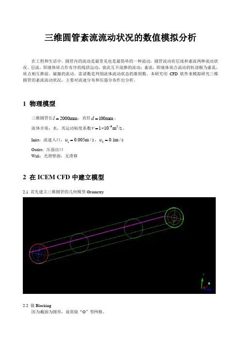
1 物理模型三维圆管长2000mm l =,直径100mm d =。
流体介质:水,其运动粘度系数62110m /s ν-=⨯。
Inlet :流速入口,10.005m /s υ=,20.1m /s υ= Outlet :压强出口Wall :光滑壁面,无滑移2 在ICEM CFD 中建立模型2.1 首先建立三维圆管的几何模型Geometry2.2 做Blocking因为截面为圆形,故需做“O ”型网格。
2.3 划分网格mesh注意检查网格质量。
在未加密的情况下,网格质量不是很好,如下图因管流存在边界层,故需对边界进行加密,网格质量有所提升,如下图2.4 生成非结构化网格,输出fluent.msh 等相关文件3 数值模拟原理紊流流动当以水流以流速20.1m /s υ=,从Inlet 方向流入圆管,可计算出雷诺数10000υdRe ν==,故圆管内流动为紊流。
假设水的粘性为常数(运动粘度系数62110m /s ν-=⨯)、不可压流体,圆管光滑,则流动的控制方程如下:①质量守恒方程:()()()0u v w t x y zρρρρ∂∂∂∂+++=∂∂∂∂ (0-1)②动量守恒方程:2()()()()()()()()()()[]u uu uv uw u u ut x y z x x y y z z u u v u w p x y z xρρρρμμμρρρ∂∂∂∂∂∂∂∂∂∂+++=++∂∂∂∂∂∂∂∂∂∂'''''∂∂∂∂+----∂∂∂∂ (0-2)2()()()()()()()()()()[]v vu vv vw v v v t x y z x x y y z z u v v v w px y z yρρρρμμμρρρ∂∂∂∂∂∂∂∂∂∂+++=++∂∂∂∂∂∂∂∂∂∂'''''∂∂∂∂+----∂∂∂∂ (0-3)2()()()()()()()()()()[]w wu wv ww w w w t x y z x x y y z z u w v w w px y z zρρρρμμμρρρ∂∂∂∂∂∂∂∂∂∂+++=++∂∂∂∂∂∂∂∂∂∂'''''∂∂∂∂+----∂∂∂∂ (0-4)③湍动能方程:()()()()[())][())][())]t t k k t k k k ku kv kw k k t x y z x x y yk G z zμμρρρρμμσσμμρεσ∂∂∂∂∂∂∂∂+++=+++∂∂∂∂∂∂∂∂∂∂+++-∂∂ (0-5)④湍能耗散率方程:212()()()()[())][())][())]t t k k t k k u v w t x y z x x y y C G C z z k kεεμμρερερερεεεμμσσμεεεμρσ∂∂∂∂∂∂∂∂+++=+++∂∂∂∂∂∂∂∂∂∂+++-∂∂ (0-6)式中,ρ为密度,u 、ν、w 是流速矢量在x 、y 和z 方向的分量,p 为流体微元体上的压强。
1 FLUENT 的求解计划对于需要使用FLUENT求解问题时,就需要按照一定的思路对我们所要求解的具体问题进行分析,制定合理的求解方法。
其主要包括以下四部分:A、计算目标的选定——通过FLUENT的计算需要得到什么样的结果,需要怎样的模型精度,如何利用这些结果得到我们需要的实际情况。
B、计算模型的选择——将实际物理模型系统进行抽象性简化,确定计算域,选定计算域的边界条件,定义模型2D或3D构造。
C、物理模型的选择——对所要模拟的物理模型设置具体的计算模型,例如湍流模型,是否为稳态,是否可压缩,是否具有能量交换等。
D、求解过程的选定——确定是否运用求解器现有公式及算法直接进行求解,或更改其他参数设置,加速计算的收敛。
2 Gambit简介Gambit是FLUENT公司于98年推出的前处理网格生成软件,用于物理模型的建立和网格的划分。
它是数值模拟过程的第一个重要环节,其建模与网格的划分过程属于数值模拟的前处理过程,其中建模是物理空间到计算空间的映射过程,网格划分则是对连续空的离散化过程。
建模的形式有很多种,包括solidworks、CAD、Pro/E等。
Gambit作为Fluent公司开发的前处理软件,在集合建模和导入方面,他具备ACIS实体建模能力。
Gambit软件主要分为以下四个步骤:A、构造几何模型通过Gambit建模工具绘制几何模型,或利用CAD生成的模型导入。
B、划分网格及检查质量对所绘制几何模型进行网格划分,并检查网格质量。
C、制定边界类型和区域类型指定网格模型中的各边界类型及存在多个区域时的区域类型。
D、输出模型导出以上所建立的几何模型,进而导入Fluent求解器中进行计算。
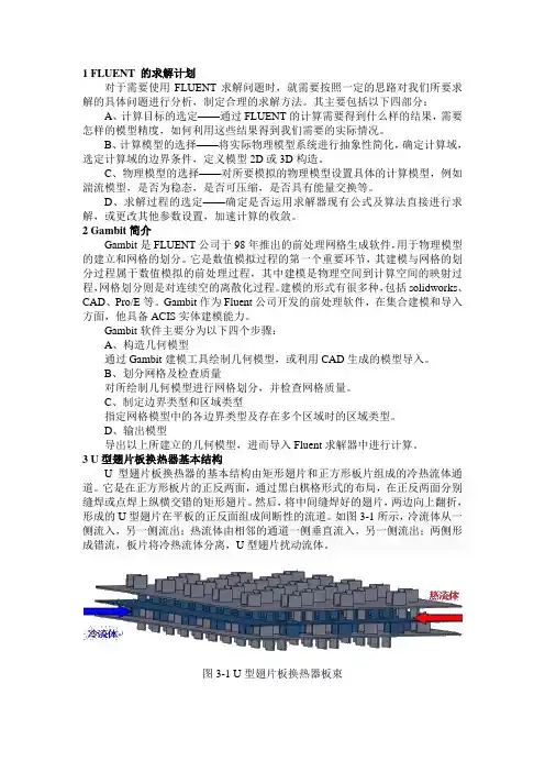
3 U型翅片板换热器基本结构U型翅片板换热器的基本结构由矩形翅片和正方形板片组成的冷热流体通道。
它是在正方形板片的正反两面,通过黑白棋格形式的布局,在正反两面分别缝焊或点焊上纵横交错的矩形翅片。
然后,将中间缝焊好的翅片,两边向上翻折,形成的U型翅片在平板的正反面组成间断性的流道。
fluent 燃烧算例
本文介绍了fluent软件在燃烧流动领域的应用算例。
首先介绍了燃烧流动的基本概念和fluent软件的基本使用方法,然后通过具体的算例来展示 fluent 软件在燃烧流动中的应用。
算例一:气体燃烧室内部流动分析。
通过建立三维模型,使用fluent 软件对燃烧室内部的流动进行模拟和分析,得到了室内流场的速度分布、温度分布等参数,为燃烧过程的优化和控制提供了重要的参考和依据。
算例二:柴油机燃烧过程的数值模拟。
通过建立柴油机的三维模型,结合燃油喷射的过程和燃烧反应机理,使用 fluent 软件对柴油机燃烧过程进行数值模拟,得到了燃烧的温度、压力、速度、质量分数等相关参数,为柴油机的性能优化和燃烧控制提供了重要的参考和依据。
算例三:天然气管道燃烧事故的模拟分析。
通过建立天然气管道的三维模型,结合管道内的燃烧反应机理,使用 fluent 软件对天然气管道的燃烧事故进行模拟和分析,得到了燃烧事故的发展过程、温度、压力等参数,为燃气安全事故的预防和控制提供了重要的参考和依据。
以上三个算例展示了 fluent 软件在燃烧流动领域的广泛应用和高效性能,为燃烧流动领域的研究和实践提供了重要的工具和技术支持。
- 1 -。

FLUENT仿真计算教程主要包含以下几个步骤:
打开FLUENT软件,选择相应的版本和求解器,然后创建新的模拟项目。
导入模型和网格文件。
在FLUENT中,可以使用Gambit或ANSYS ICEM CFD等前处理软件生成网格文件,并将其导入到FLUENT中。
在FLUENT中设置模型参数和边界条件。
例如,可以设置流体物性、流动条件(如速度、压力等)以及热力学条件等。
初始化模拟并运行模拟。
在运行模拟之前,可以设置求解器参数、迭代次数、收敛准则等。
检查模拟结果。
在模拟完成后,可以在FLUENT中查看结果,如速度场、压力场、温度场等。
同时,也可以使用后处理功能对结果进行进一步的分析和可视化。
导出模拟结果。
在FLUENT中,可以将结果导出为各种格式的文件,如ASCII、二进制等。
需要注意的是,在进行FLUENT仿真计算时,需要具备一定的流体动力学和数值计算基础,以及对所研究问题的深入理解。
同时,还需要对所使用的软件和工具进行充分的了解和熟悉。
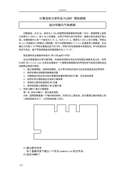
计算流体力学作业FLUENT 模拟燃烧问题描述:长为2m、直径为0.45m的圆筒形燃烧器结构如图1所示,燃烧筒壁上嵌有三块厚为0.0005 m,高0.05 m的薄板,以利于甲烷与空气的混合。
燃烧火焰为湍流扩散火焰。
在燃烧器中心有一个直径为0.01 m、长为0.01 m、壁厚为0.002 m的小喷嘴,甲烷以60 m/s的速度从小喷嘴注入燃烧器。
空气从喷嘴周围以0.5 m/s的速度进入燃烧器。
总当量比大约是0.76(甲烷含量超过空气约28%),甲烷气体在燃烧器中高速流动,并与低速流动的空气混合,基于甲烷喷嘴直径的雷诺数约为5.7×10³。
假定燃料完全燃烧并转换为:CH4+2O2→CO2+2H2O反应过程是通过化学计量系数、形成焓和控制化学反应率的相应参数来定义的。
利用FLUENT的finite-rate化学反应模型对一个圆筒形燃烧器内的甲烷和空气的混合物的流动和燃烧过程进行研究。
1、建立物理模型,选择材料属性,定义带化学组分混合与反应的湍流流动边界条件2、使用非耦合求解器求解燃烧问题3、对燃烧组分的比热分别为常量和变量的情况进行计算,并比较其结果4、利用分布云图检查反应流的计算结果5、预测热力型和快速型的NO X含量6、使用场函数计算器进行NO含量计算一、利用GAMBIT建立计算模型第1步启动GAMBIT,建立基本结构分析:圆筒燃烧器是一个轴对称的结构,可简化为二维流动,故只要建立轴对称面上的二维结构就可以了,几何结构如图2所示。
(1)建立新文件夹在F盘根目录下建立一个名为combustion的文件夹。
(2)启动GAMBIT(3)创建对称轴①创建两端点。
A(0,0,0),B(2,0,0)②将两端点连成线(4)创建小喷嘴及空气进口边界①创建C、D、E、F、G点C D E F Gx 0 0.01 0.01 0 0y 0.005 0.005 0.007 0.007 0.225②连接AC、CD、DE、DF、FG。
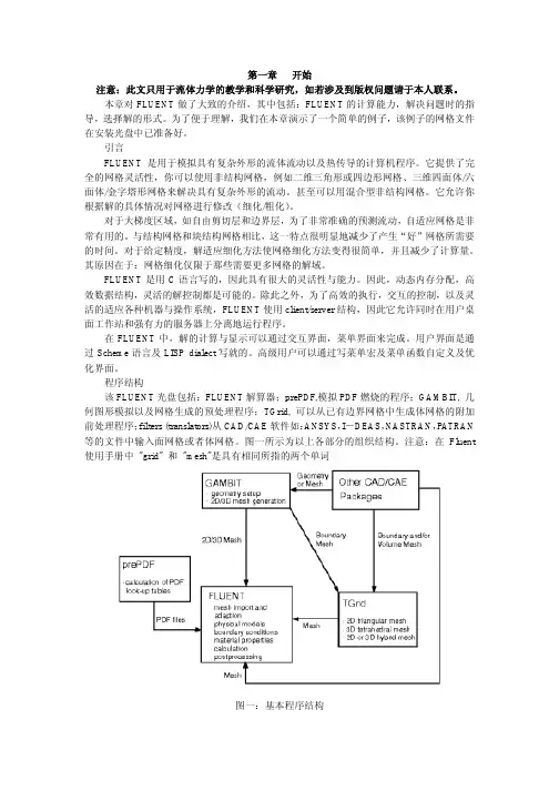
第一章开始注意:此文只用于流体力学的教学和科学研究,如若涉及到版权问题请于本人联系。
本章对FLUENT做了大致的介绍,其中包括:FLUENT的计算能力,解决问题时的指导,选择解的形式。
为了便于理解,我们在本章演示了一个简单的例子,该例子的网格文件在安装光盘中已准备好。
引言FLUENT是用于模拟具有复杂外形的流体流动以及热传导的计算机程序。
它提供了完全的网格灵活性,你可以使用非结构网格,例如二维三角形或四边形网格、三维四面体/六面体/金字塔形网格来解决具有复杂外形的流动。
甚至可以用混合型非结构网格。
它允许你根据解的具体情况对网格进行修改(细化/粗化)。
对于大梯度区域,如自由剪切层和边界层,为了非常准确的预测流动,自适应网格是非常有用的。
与结构网格和块结构网格相比,这一特点很明显地减少了产生“好”网格所需要的时间。
对于给定精度,解适应细化方法使网格细化方法变得很简单,并且减少了计算量。
其原因在于:网格细化仅限于那些需要更多网格的解域。
FLUENT是用C语言写的,因此具有很大的灵活性与能力。
因此,动态内存分配,高效数据结构,灵活的解控制都是可能的。
除此之外,为了高效的执行,交互的控制,以及灵活的适应各种机器与操作系统,FLUENT使用client/server结构,因此它允许同时在用户桌面工作站和强有力的服务器上分离地运行程序。
在FLUENT中,解的计算与显示可以通过交互界面,菜单界面来完成。
用户界面是通过Scheme语言及LISP dialect写就的。
高级用户可以通过写菜单宏及菜单函数自定义及优化界面。
程序结构该FLUENT光盘包括:FLUENT解算器;prePDF,模拟PDF燃烧的程序;GAMBIT, 几何图形模拟以及网格生成的预处理程序;TGrid, 可以从已有边界网格中生成体网格的附加前处理程序;filters (translators)从CAD/CAE软件如:ANSYS,I-DEAS,NASTRAN,PATRAN 等的文件中输入面网格或者体网格。

FLUENT 12 模拟步骤Problem Setup读入网格:file read case 选择网格文件(后缀为。
Mesh)1 General1)Mesh(网格)> Check(点击查看网格的大致情况,如有无负体积等)Maximum volume (m3)(最大体积,不能为负)Minimum volume (m3)(最小体积,不能为负)Total volume (m3)(总体体积,不能为负)> Report Quality(点击报告网格质量)Maximum cell squish(最大单元压扁,如果该值等于1,表示得到了很坏的单元)Maximum cell skewness(最大单元扭曲,该值在0到1之间,0表示最好,1表示最坏)Maximum aspect ratio(最大长宽比,1表示最好)> Scale(点击缩放网格尺寸,FLUENT默认的单位是米)Mesh Was Create In(点选mm →点击Scale按钮且只能点击一次)View Length Unit In(点选mm →直接点击Close按钮不能再点击Scale按钮)> Display(点击显示网格设定)→弹出Mesh Colors窗口Options(选Edges和Faces)Edge Type(点选All)Surface(点选曲面)→点击Display按钮点击Colors按钮→弹出Mesh Display窗口Options(点选Color by ID)→点击Close按钮→再点击Display按钮2)Solver(求解器)> Pressure-Based(压力基,压力可变,用于低速不可压缩流动)> Density-Based(密度基,密度可变,用于高速可压缩流动)3)Velocity Formulation(速度格式)> Absolute(绝对速度)> Relative(相对速度)4)Time(时间)> Steady(稳态)> Transient(瞬态)5)Units(点击设置变量单位)点击按钮→弹出Set Units窗口→在Quantities项里点选pressure →在Units项里点选atm →点击New按钮→点击OK按钮→点击Close按钮2 Models(物理模型)1)Multiphase(多相流模型)2)Energy(能量方程,一般要双击勾选)3)Viscous(粘性模型,一般选k-ε模型,所有参数保持默认设置)4)Radiation(辐射模型)5)Heat Exchanger(传热模型)6)Species(组分模型)7)Discrete Phase(离散相模型)8)Solidification & Melting(凝固与融化模型)9)Acoustics(声学模型,一般选择Broadband Noise Source模型,所有参数保持默认设置)3 Materials(定义材料)1)点击FLUENT Database →在FLUENT Fluid Materials里选择所需要的物质→点击Copy按钮→点击Close按钮→再点击Change/Create按钮2)点击User-Defined Database →选定写好的自定义文件→点击OK按钮3)自定义材料物性参数:在Name文本框中输入自定义材料名字gas →Chemical Formula文本框删除为空→修改Properties中各参数的值→点击Change/Create按钮→弹出Change/Create mixture and Overwrite air对话框→点击NO按钮→点击Close按钮4 Phases(相)5 Cell Zone Conditions(单元区域条件)点击Edit按钮→在Material Name项的下拉列表中选择gas(工作介质)→点击OK按钮6 Boundary Conditions(边界条件)1)Pressure-Inlet(压力进口)> Momentum(动量)Reference Frame(参考系)Gauge Total Pressure(总表压)Supersonic/Initial Gauge Pressure(初始表压或静压,一般比总表压小500Pa左右,或设为出口表压)Direction Specification Method(进口流动方向指定方法,Normal to Boundary垂直边界)Turbulence > Specification Method(湍流指定方法,Intensity and Hydraulic Diameter)Turbulent Intensity(湍流强度,一般为1)Hydraulic Diameter(水力半径,一般为管内径)> Thermal(热量)Total Temperature(总温)> Species(组分)2)Pressure -Outlet(压力出口)> Momentum(动量)Gauge Pressure(表压)Backflow Direction Specification Method(回流方向指定方法)Radial Equilibrium Pressure Distribution(径向平衡压力分布)Target Mass Flow Rate(目标质量流率)Non-Reflecting Boundary(非反射边界)Turbulence > Specification Method(湍流指定方法,点选Intensity and Hydraulic Diameter)Backflow Turbulent Intensity(回流湍流强度,一般为1)Backflow Hydraulic Diameter(回流水力半径,一般为管内径)> Thermal(热量)Backflow Total Temperature(回流总温)> Species(组分)7 Mesh Interfaces(分界面网格)8 Reference Values(参考值)9 Adapt(自适应)Adapt →Gradient(压力梯度自适应)> Options(显示选项)Refine(加密,勾选)Coarsen(粗糙,勾选)Normalize(正规化)> Method(方法)Curvature(曲率)Gradient(梯度,勾选)Iso-Value(等值)> Gradient of(梯度变量)Pressure(压力,点选)Static pressure(静压,点选)> Normalization(正常化)Standard(标准)Scale(可缩放,勾选)Normalize(使正常化)> Coarsen Threshold(粗糙比,0.3)> Refine Threshold(细化比,0.7)> Dynamic(动态)Dynamic(动态,勾选)Interval(每隔几次迭代自适应一次)→点击Mark按钮→点击Adapt按钮→(点击Compute按钮)→点击Apply按钮Solution1 Solution Methods(求解方法)1)Formulation(求解格式,默认为隐式Implicit)2)Flux Type(通量类型,默认为Roe-FDS)3)Gradient(求解格式,默认为Least Squares Cell Based)4)Flow(流动,点选二阶迎风格式Second Order Upwind)5)Turbulent Kinetic Energy(湍动能,点选二阶迎风格式Second Order Upwind)6)Turbulent Dissipation Rate(湍流耗散率,点选二阶迎风格式Second Order Upwind)2 Solution Controls1)Courant Number(库朗数,控制时间步长,瞬态计算才需要设置)2)Un-Relaxation Factors(欠松弛因子)> Turbulent Kinetic Energy(湍动能,默认为0.8)> Turbulent Dissipation Rate(湍流耗散率,默认为0.8)> Turbulent Viscosity(湍流粘度,默认为1)3)Equations(点击弹出控制方程)> Turbulence(湍流方程)> Flow(流动方程= 连续方程+ 动量方程+ 能量方程)4)Limits(点击弹出限制窗口)对某些变量使用限制值,如果计算的某个变量值小于最小限制值,则求解器就会用相应的极限取代计算值。

某三轴mw级燃气轮机热力循环计算的建模及验证燃气轮机在当今世界是能源动力的重要来源,并受到越来越多关注。
考虑到功率发电设备的经济性和安全性,将燃气轮机中的温度、压力循环进行建模和数字仿真是保障此类动力设备安全运行与提高经济效益的有效手段。
本文就以某三轴mw级燃气轮机为研究对象,采用Fluent软件进行热流计算的模拟计算,建立热流模型,以较好的精度和可靠性对其热力循环进行模拟应用。
一、热力循环模型构建热力循环模型构建包括流动和热传输模型,分别使用流水线和热模拟计算方法来建立模型。
流体模型,采用了RNG k-ε流动模型,这是一种常用的k-ε模型,属于二维湍流模型;当能量和质量计算方数不严格时,使用一维模型简化计算可以得到更高的计算精度和效率。
热模型采用的是瞬态传热模型,这是一种常用的热传输模型,根据热流量物理特性,通过模型将运动分析结果结合热传输方程,模拟实际热传输中的温度场,以精确地模拟热力特性。
二、计算结果与分析建模完毕后,运用计算模型对某mw级燃气轮机进行热力循环建模、验证和优化,最终得出结果如下:1.在燃气轮机的排气和热耗端的温度差异充分体现了热流的分布特征;排气端的温度达到最高,热耗端的温度最低。
热流的变化趋势和计算均体现出燃气轮机的温度特征。
2.燃气轮机中的压力变化分别表现为增大和减小,排气和热耗端的压力分布差异明显,且和计算值基本一致。
3.结果同时较好地反映了燃气轮机同步发电过程中物理特征及其变化规律,可用作模拟及优化设计的参考。
经过验证,研究的模型可以准确的模拟燃气轮机的运行状况,有效地建立了热力循环的模型,为燃气轮机系统的优化控制提供证据,也可以为安全运行提供指导。
三、结论本文针对某三轴mw级燃气轮机,利用Fluent软件对其热力循环进行建模,计算得到结果较为满意,为其优化设计和安全运行提供了参考依据,为燃气轮机有效运行提供了重要的理论支撑。
但本文仍有一定的局限性,例如仅针对某种规格的燃气轮机,在建模过程中只考虑了温度和压力两个参数,未考虑流场分布特征等。
计算流体力学作业FLUENT 模拟燃烧
一、模拟对象描述
圆柱型火焰燃烧器的结构图1所示。
火焰是湍流扩散火焰,在进口的中心处有一个小喷嘴。
甲烷以80m/s的速度从小喷嘴中射入,周围空气以0.5m/s 的速度流入燃烧器,过量空气系数为1.28。
在甲烷和空气之间用一层外墙隔开。
甲烷流动的雷诺数为5700.甲烷与空气的反应采用最常见的单步总包反应,而且认为反应是扩散控制的,因此使用涡耗散模型对其进行模拟。
图1 二维湍流扩散燃烧器中甲烷空气燃烧
二、实例操作步骤
1.利用GAMBIT建立计算区域和指定边界条件类型。
2.利用FLUENT求解器求解
步骤1:网格的相关操作
启动二维FLUENT,在菜单中点击File-Read-Case…,在相应目录中,找到自己生成的gascomb.msh。
点击Grid-Check,检查网格。
点击Grid-Scale…,设定网格尺寸,将网格改为按毫米生成。
点击Grid-Check,检查一下计算域是否正确:X的最大值是1.8,Y的最大值是0.225.然后关闭对话框。
点击Display-Grid…显示网格
步骤2:模型的设定
步骤3:材料属性设定
步骤4边界条件的设定
步骤5:设定初始条件和其他求解控制参数设置
残差随迭代逐渐收敛情况步骤6:结果显示
温度等值线云图。
Ansys Fluent基础详细入门教程(附简单算例)当你决定使FLUENT解决某一问题时,首先要考虑如下几点问题:定义模型目标:从CFD模型中需要得到什么样的结果?从模型中需要得到什么样的精度;选择计算模型:你将如何隔绝所需要模拟的物理系统,计算区域的起点和终点是什么?在模型的边界处使用什么样的边界条件?二维问题还是三维问题?什么样的网格拓扑结构适合解决问题?物理模型的选取:无粘,层流还湍流?定常还是非定常?可压流还是不可压流?是否需要应用其它的物理模型?确定解的程序:问题可否简化?是否使用缺省的解的格式与参数值?采用哪种解格式可以加速收敛?使用多重网格计算机的内存是否够用?得到收敛解需要多久的时间?在使用CFD分析之前详细考虑这些问题,对你的模拟来说是很有意义的。
第01章fluent介绍及简单算例 (2)第02章fluent用户界面22 (3)第03章fluent文件的读写 (5)第04章fluent单位系统 (8)第05章fluent网格 (10)第06章fluent边界条件 (36)第07章fluent流体物性 (55)第08章fluent基本物理模型 (63)第11章传热模型 (75)第22章fluent 解算器的使用 (82)第01章fluent介绍及简单算例FLUENT是用于模拟具有复杂外形的流体流动以及热传导的计算机程序。
对于大梯度区域,如自由剪切层和边界层,为了非常准确的预测流动,自适应网格是非常有用的。
FLUENT解算器有如下模拟能力:●用非结构自适应网格模拟2D或者3D流场,它所使用的非结构网格主要有三角形/五边形、四边形/五边形,或者混合网格,其中混合网格有棱柱形和金字塔形。
(一致网格和悬挂节点网格都可以)●不可压或可压流动●定常状态或者过渡分析●无粘,层流和湍流●牛顿流或者非牛顿流●对流热传导,包括自然对流和强迫对流●耦合热传导和对流●辐射热传导模型●惯性(静止)坐标系非惯性(旋转)坐标系模型●多重运动参考框架,包括滑动网格界面和rotor/stator interaction modeling的混合界面●化学组分混合和反应,包括燃烧子模型和表面沉积反应模型●热,质量,动量,湍流和化学组分的控制体源●粒子,液滴和气泡的离散相的拉格朗日轨迹的计算,包括了和连续相的耦合●多孔流动●一维风扇/热交换模型●两相流,包括气穴现象●复杂外形的自由表面流动上述各功能使得FLUENT具有广泛的应用,主要有以下几个方面●Process and process equipment applications●油/气能量的产生和环境应用●航天和涡轮机械的应用●汽车工业的应用●热交换应用●电子/HV AC/应用●材料处理应用●建筑设计和火灾研究总而言之,对于模拟复杂流场结构的不可压缩/可压缩流动来说,FLUENT是很理想的软件。
应用FLUENT进行射流流场的数值模拟谢峻石何枫清华大学工程力学系一.引言射流是流体运动的一种重要类型,射流的研究涉及到许多领域,如热力学、航空航天学、气象学、环境学、燃烧学、航空声学等。
在机械制造与加工的过程中,就经常利用压缩空气喷枪喷射出高速射流进行除尘、除水、冷却、雾化、剥离、引射等。
在工业生产中,改善气枪喷嘴的设计,提高气枪的工作效率对于节约能源具有重大的意义。
FLUENT是目前国际上比较流行的商用CFD软件包,它具有丰富的物理模型、先进的数值方法以及强大的前后处理功能,在航空航天、汽车设计、石油天然气、涡轮机设计等方面都有着广泛的应用。
本文的工作就是将FLUENT应用于喷嘴射流流场的数值模拟,使我们更加深刻地理解问题产生的机理、为实验研究提供指导,节省实验所需的人力、物力和时间,并对实验结果的整理和规律的得出起到很好的指导作用.。
二.控制方程与湍流模式非定常可压缩的射流满足如下的N-S方程:(1)上式中,量,H是源项。
是控制体,是控制体边界面,W是求解变量,F是无粘通量,G 是粘性通采用二阶精度的有限体积法对控制方程进行空间离散,时间离散采用Gauss-Seidel隐式迭代。
FLUENT软件包中提供了S-A(Spalart-Allmaras),K-Realizable K-选择RNG K-(包括标准K-、RNG K-和),Reynolds Stress等多种湍流模式,本文在大量数值实验的基础上,亚音速射流湍流模式,超音速射流选择S-A湍流模式。
三.算例分析(一)二维轴对称亚声速自由射流计算了一个出口直径为3mm的轴对称收缩喷嘴的亚声速射流流场,压比为1.45。
外流场的计算域为20D×5D(见图1)。
图1 计算域及网格示意图图2显示的是速度分布,图3、图4分别显示了轴线上的速度分布以及截面上的速度分布计算值与实验值的比较。
从图中可以看出,亚声速自由射流轴线上的速度核心区的长度约为5~6D,计算值与实验值吻合的比较一致,证明RNG k-模拟。
1.GAMBIT建模(1)操作1;双击桌面“GAMBIT快捷方式”进入操作空间,如下图图1几何模型创建遵循原则:按组成几何模型的几何拓扑结构,由低层向高层创建,即按由点到面,再到体的顺序创建(这样减的好处是便于网格的划分和Fluent求解时边界条件的设定,缺点是步骤繁琐)。
对于较简单的模型,可省略低拓扑结构,直接建立最终模型。
(2)创建节点操作2:鼠标左键依次单击Operation Geometry进入下图图2操作3:左键单击上图Apply,创建第一个点(坐标(0、0、0)),如下图,可以发现坐标原点显示白色图3操作4:在上图2中Global下输入x:200,y:0,z: 0,左键单击Apply, 如下图,操作5:左键单击(作用:窗口显示),如下图重复操作4和操作5,以此建立点(0,-0.0025,0)、(0.05,-0.0025,0)、(0.05、-0.0125)(0.15,0.0025,0),(0.15,0.0125,0),(0.2,0.0025),如下图,(3)节点成线操作1:左键依次单击,然后Shift+鼠标左键依次(为沿围成图形各点顺序)单击所创建的点,如下图,左键单击Apply,如下图,(4)连线成面操作1:左键单击,Shift+左键依次单击图中各线段,如下图,左键单击Apply,如下图,(5)网格划分网格划分遵循原则与模型创建类似操作1:左键依次单击,如下图,操作2:Shift+左键选中模型中一条边操作3:左键单击,弹出菜单中选择interval count,在左侧输入框中输入;200(为该条边上网格节点数),如下图重复操作2和操作3,将沿y方向的短边和长边节点数分别设定为20和80.注意:对于相互平行两边,节点设置可只在一边进行;如果两边均设定,切记两边节点数要一致。
操作4:左键单击,Shift+左键单击图中任一边,所有边显示红色,然后左键单击Apply,如下图,(6)设置边界类型操作1: 左键单击,如下图,操作2:Shift+左键单击模型最左侧沿y方向的短边(显红色),单击,弹出菜单中选择PRESSURE-INLET,左键单击Apply,如下图,操作3:Shift+左键单击模型最右侧沿y方向的短边(显红色),单击,弹出菜单中选择PRESSURE-OUTLET,左键单击Apply,如下图,操作4:其它边不设置,默认为壁面条件。
Fluent验证案例15:发动机缸内流动本验证案例计算发动机缸内流体流动。
1问题描述本案例较为简单,计算几何如下图所示。
计算模拟理想的发动机气缸内流动情况,计算域包含一个直进口及一个升程10 mm的阀门。
采用3D几何模型、稳态等温及不可压缩模拟,利用标准k-epsilon湍流模型及标准壁面函数进行计算。
2Fluent设置•以3D、Double Precision启动Fluent•利用菜单File → Read → Case...加载文件valve10-1.cas.gz2.1 General设置•鼠标双击模型树节点General,右侧面板保持默认设置2.2 Models设置•右键选择模型树节点Models > Viscous,选择菜单项Model → Standard k-epsilon激活湍流模型2.3 Materials设置•创建材料fluid,设置其density = 894 kg/m3,Viscosity = 0.00152875 kg/m-s2.4 Cell Zone Conditions•鼠标双击模型树节点Cell Zone Conditions > fluid-11,弹出对话框中设置Materials Name为fluid2.5 Boundary Conditions设置•鼠标双击模型树节点Boundary Conditions > velocity-inlet-1 •设置Velocity Magnitude为0.928156 m/s•设置湍流强度为10%,湍流尺度为0.28 m出口边界采用默认设置。
2.6 Monitor•鼠标双击模型树节点Monitor > Residual,弹出对话框中设置连续方程收敛残差为1e-5,如下图所示2.6 Initialzation•右键选择模型树节点Initialization,点击菜单项Initialize进行初始化2.7 Run Calculation•双击模型树节点Run Calculation,右侧面板设置Number of Iterations为1000•点击按钮Calculate开始计算3计算结果验证•x=0面上速度分布网格有点儿粗糙,导致云图出现不连续的情况。
Fluent仿真计算问题描述:一个冷、热水混合器的内部流动与热量交换的问题。
温度为350K的热水自上部的热水小管流入,与下部右侧小管嘴流入290K 的冷水在混合器内进行热量与动量的交换后,自下部左侧的小管流出。
一、前处理——利用GAMBIT建立计算模型。
针对所描述的问题利用GAMBIT建立模型并输出网格。
第1步创建坐标网格图操作:TOOLS→COORDINATEJ→DISPLAYGRID第2步由节点创建直线(1)隐藏坐标网格操作:在显示设置对话框中,使Visibility 选项的左边按钮呈非选中状态;点击Apply(2)由节点连接成直线(边界线)操作:GEOMETRY→EDGE→CREATE EDGE→STRAIGHT第3步创建圆弧边操作:GEOMETR→YEDE→CREATE EDGE第4步创建小管嘴(1)创建小管嘴入口边节点操作:GEOMETRY→VERTEX→MOVE/COPY VERTICES,打开移动/复制节点对话框(2)创建小管嘴的边线操作:GEOMETRY→EDGE→CREATEEDGE第5步由线组成面操作:GEOMETRY→FACE→FORM FACE打开创建面对话框,本模型有四个面,应分别创建。
首先创建主题面,然后再逐一的建立三个小管嘴的面。
第6步确定边界线的内部节点分布并创建面网格第7步设置边界类型1、关闭网格显示2、设置边界类型操作:ZONES →SPECIFY BOUNDARY TYPES,打开定义边界类型对话框。
(1)设置下方右侧的小管嘴入口截面为速度边界(边线st)(2)设置上边的小管嘴入口截面为速度边界(边线uv)(3)设置下方左侧的小管嘴截面为压力初六边界(边线pq)(4)按下shift+鼠标左键,点击边界线pq第8步输出网格并保存文件(1)输出网格操作:FILE→EXPORT→MESH打开输出网格文件对话框。
如下图,即完成了网格文件的输出操作。
(2)保存GAMBIT文件,并推出GAMBIT操作:FILE→EXIT二、利用FLUENT进行混合器内流动与换热的仿真计算第1步启动FLUENT-2d(1)启动FLUENT-2d求解器(2)读入网格文件like.mesh操作:file→read→case...(3)网格检查操作:grid →check(4) 网格信息操作:grid →info →size(5)平滑(交换)网格这一步是为确保网格质量的操作。
ing Sliding MeshesIntroductionThe analysis of turbomachinery often involves the examination of the unsteady effects due toflow interaction between the stationary components and the rotating blades.In this tutorial,the sliding mesh capability of FLUENT is used to to analyze the unsteady flow in an axial compressor stage.The rotor-stator interaction is modeled by allowing the mesh associated with the rotor blade row to rotate relative to the stationary mesh associated with the stator blade row.This tutorial demonstrates how to do the following:•Create periodic zones.•Set up the unsteady solver and boundary conditions for a sliding mesh simulation.•Set up the grid interfaces for a periodic sliding mesh model.•Sample the time-dependent data and view the mean value.PrerequisitesThis tutorial assumes that you are familiar with the menu structure in FLUENT and that you have completed Tutorial1.Some steps in the setup and solution procedure will not be shown explicitly.Problem DescriptionThe model represents a single-stage axial compressor comprised of two blade rows.The first row is the rotor with16blades,which is operating at a rotational speed of37,500 rpm.The second row is the stator with32blades.The blade counts are such that the domain is rotationally periodic,with a periodic angle of22.5degrees.This allows you to model only a portion of the geometry,namely,one rotor blade and two stator blades.Due to the high Reynolds number of theflow and the relative coarseness of the mesh (both blade rows are comprised of only13,856cells total),the analysis will employ the inviscid model,so that FLUENT is solving the Euler equations.Using Sliding MeshesoutletFigure11.1:Rotor-Stator Problem DescriptionUsing Sliding MeshesSetup and SolutionPreparation1.Download sliding_mesh.zip from the Fluent er Services Center or copyit from the FLUENT documentation CD to your working folder(as described inTutorial1).2.Unzip sliding_mesh.zip.axial comp.msh can be found in the sliding mesh folder created after unzippingthefile.3.Start the3D(3d)version of FLUENT.Step1:Grid1.Read in the meshfile axial comp.msh.File−→Read−→Case...2.Check the grid.Grid−→CheckFLUENT will perform various checks on the mesh and will report the progress inthe console.Pay particular attention to the minimum volume,and make sure thisis a positive number.Warnings will be displayed regarding unassigned interface zones,resulting in thefailure of the grid check.You do not need to take any action at this point,as thisissue will be rectified when you define the grid interfaces in a later step.Using Sliding Meshes3.Define the units for the grid.Define−→Units...(a)Select angular-velocity in the Quantities selection list.(b)Select rpm in the Units selection list.(c)Select pressure in the Quantities selection list.(d)Select atm in the Units selection list.(e)Close the Set Units panel.4.Display the grid(Figure11.2).Display−→Grid...Using Sliding Meshes(a)Retain the default selections in the Surfaces selection list.(b)Click Display and close the Grid Display panel.(c)Rotate the view to get the display shown in Figure11.2.Figure11.2:Rotor-Stator Outline DisplayThe inlet to the rotor mesh is colored blue,the interface between the rotor and stator meshes is colored yellow,and the outlet of the stator mesh is colored red.e the text user interface to change zones rotor-per-1and rotor-per-3fromwall zones to periodic zones.(a)Press<Enter>in the console to get the command prompt(>).(b)Type the commands shown in boxes as follows:Using Sliding Meshes>grid/grid>modify-zones/grid/modify-zones>list-zonesid name type material kind -----------------------------------------------------------------------13fluid-rotor fluid air cell 28fluid-stator fluid air cell 2default-interior:0interior face 15default-interior interior face 3rotor-hub wall aluminum face 4rotor-shroud wall aluminum face 7rotor-blade-1wall aluminum face 8rotor-blade-2wall aluminum face 16stator-hub wall aluminum face 17stator-shroud wall aluminum face 20stator-blade-1wall aluminum face 21stator-blade-2wall aluminum face 22stator-blade-3wall aluminum face 23stator-blade-4wall aluminum face 5rotor-inlet pressure-inlet face 19stator-outlet pressure-outlet face 10rotor-per-1wall aluminum face 12rotor-per-2wall aluminum face 24stator-per-2wall aluminum face 26stator-per-1wall aluminum face 6rotor-interface interface face 18stator-interface interface face 11rotor-per-4wall aluminum face 9rotor-per-3wall aluminum face 25stator-per-4wall aluminum face 27stator-per-3wall aluminum face /grid/modify-zones>make-periodicPeriodic zone[()]10Shadow zone[()]9Rotational periodic?(if no,translational)[yes]yesCreate periodic zones?[yes]yesall176faces matched for zones10and9.zone9deletedcreated periodic zones.Using Sliding Meshes6.Similarly,change the following wall zone pairs to periodic zones:Zone Pairs Respective Zone IDsrotor-per-2and rotor-per-412and11stator-per-1and stator-per-326and27stator-per-2and stator-per-424and25Step2:Models1.Define the solver settings.Define−→Models−→Solver...(a)Select Density Based from the Solver group box.(b)Retain the selection of Green-Gauss Cell Based from the Gradient Option groupbox.(c)Retain the selection of Implicit from the Formulation list.(d)Select Unsteady from the Time list.(e)Select2nd-Order Implicit from the Unsteady Formulation list.(f)Click OK to close the Solver panel.Using Sliding Meshes2.Enable the inviscid model.Define−→Models−→Viscous...(a)Enable Inviscid.(b)Click OK.Using Sliding MeshesStep3:Materials1.Specify air(the default material)as thefluid material,using the ideal gas law tocompute density.Define−→Materials...(a)Retain the default entry of air in the Name text entryfield.(b)Select ideal-gas from the Density drop-down list in the Properties group box.(c)Retain the default values for all other properties.(d)Click Change/Create and close the Materials panel.Using Sliding MeshesStep4:Operating Conditions1.Set the operating pressure.Define−→Operating Conditions...(a)Enter0atm for the Operating Pressure.(b)Click OK to close the Operating Conditions panel.Since you have set the operating pressure to zero,you will specify the boundarycondition inputs for pressure in terms of absolute pressures when you define themin a later step.Boundary condition inputs for pressure should always be relative tothe value used for operating pressure.Step5:Boundary ConditionsDefine−→Boundary Conditions...1.Set the boundary conditions for thefluid in the rotor(fluid-rotor).(a)Make sure that(0,0,1)is entered for X,Y,and Z under Rotation-Axis Direction.(b)Select Moving Reference Frame from the Motion Type drop-down list.(c)Enter37500rpm for Speed in the Rotational Velocity group box.Scroll down tofind the Speed number-entry box.(d)Click OK to close the Fluid panel.2.Set the boundary conditions for thefluid in the stator(fluid-stator).(a)Make sure that(0,0,1)is entered for X,Y,and Z under Rotation-Axis Direction.(b)Make sure that Stationary is selected from the Motion Type drop-down list.(c)Click OK to close the Fluid panel.3.Set the boundary conditions for the inlet(rotor-inlet).(a)Enter1.0atm for the Gauge Total Pressure.(b)Enter0.9atm for the Supersonic/Initial Gauge Pressure.(c)Click the Thermal tab and enter288K for Total Temperature.(d)Click OK to close the Pressure Inlet panel.4.Set the boundary conditions for the outlet(stator-outlet).(a)Enter1.08atm for the Gauge Pressure.(b)Enable the Radial Equilibrium Pressure Distribution option.(c)Click the Thermal tab and enter288K for Backflow Total Temperature.(d)Click OK to close the Pressure Outlet panel.Note:The momentum settings and temperature you input at the pressure outlet will be used only ifflow enters the domain through this boundary.It is impor-tant to set reasonable values for these downstream scalar values,in caseflow reversal occurs at some point during the calculation.5.Retain the default boundary conditions for all wall zones.Note:For wall zones,FLUENT always imposes zero velocity for the normal velocity component,which is required whether or not thefluid zone is moving.This condition is all that is required for an inviscidflow,as the tangential velocity is computed as part of the solution.6.Close the Boundary Conditions panel.Step6:Grid Interfaces1.Create a periodic grid interface between the rotor and stator mesh regions.Define−→Grid Interfaces...(a)Enter int for Grid Interface.(b)Enable Periodic in the Interface Type group box.Enabling this option,allows FLUENT to treat the interface between the slidingand non-sliding zones as periodic where the two zones do not overlap.(c)Select rotor-interface in the Interface Zone1list.Note:In general,when one interface zone is smaller than the other,it is recommended that you choose the smaller zone as Interface Zone1.Inthis case,since both zones are approximately the same size,the order isnot significant.(d)Select stator-interface in the Interface Zone2list.(e)Click Create and close the Grid Interfaces panel.2.Check the grid again to verify that the warnings displayed earlier have been re-solved.Grid−→CheckStep7:Solution1.Set the solution parameters.Solve−→Controls−→Solution...(a)Make sure that Second Order Upwind is selected from the Flow drop-down listin the Discretization group box.(b)Click OK to close the Solution Controls panel.2.Enable the plotting of residuals during the calculation.Solve−→Monitors−→Residual...(a)Enable Plot in the Options group box.(b)Select relative from the Convergence Criterion drop-down list.(c)Enter0.01in thefields under Relative Criteria for every Residual(continuity,x-velocity,y-velocity,z-velocity,and energy).(d)Click OK to close the Residual Monitors panel.3.Enable the plotting of the data at the inlet(rotor-inlet),outlet(stator-outlet),andthe interface(stator-interface).Solve−→Monitors−→Surface...(a)Set the Surface Monitors to3.(b)Enable Plot,Print,and Write for each monitor(monitor-1,monitor-2,andmonitor-3).(c)Select Time Step from the When drop-down list for each monitor(monitor-1,monitor-2,and monitor-3).(d)Click the Define...button for monitor-1to open the Define Surface Monitorpanel.i.Select Mass Flow Rate from the Report Type drop-down list.ii.Select Flow Time from the X Axis drop-down list.iii.Select rotor-inlet from the Surfaces selection list.iv.Click OK to close the Define Surface Monitor panel.(e)Define monitor-2to report the massflow rate at the outlet(stator-outlet)asshown in the following panel:!Be sure to deselect rotor-inlet from the Surfaces selection list,before scrolling down to select stator-outlet.(f)Define monitor-3to report the area-weighted average of the static pressure atthe interface(stator-interface)as shown in the following panel:!Be sure to deselect stator-outlet from the Surfaces selection list before scrolling down to select stator-interface.(g)Click OK to close the Surface Monitors panel.4.Initialize the solution using the values at the inlet(rotor-inlet).Solve−→Initialize−→Initialize...(a)Select rotor-inlet from the Compute From drop-down list.(b)Select Absolute from the Reference Frame list.(c)Click Init and close the Solution Initialization panel.5.Save the initial casefile(axial comp.cas).File−→Write−→Case...6.Run the calculation for one revolution of the rotor.Solve−→Iterate...(a)Enter6.6666e-6s for the Time Step Size.This time step represents the length of time during which the rotor will rotate1.5degrees.Since the periodic angle of the rotor is22.5degrees,the passingperiod of the rotor blade will equal15time steps,and a complete revolution of the rotor will take240time steps.(b)Enter240for the Number of Time Steps.(c)Retain the default setting of20for the Max Iterations per Time Step in theIteration group box.(d)Click Iterate.The solution will converge in approximately3900iterations.The residuals jump at the beginning of each time step and then fall at least two to three orders of magnitude.Also,the relative convergence criteria is achieved before reaching the maximum iteration limit(20)for each time step,indicating the limit does not need to be increased.7.Examine the monitor histories for thefirst revolution of the rotor(Figures11.4,11.5,and11.6).Figure11.3:Residual History for the First Revolution ofthe RotorRevolutionFigure11.5:Mass Flow Rate at the Outlet During the FirstThe monitor histories show that large variations inflow rate and interface pressure occur early in the calculation,which are greatly reduced as time-periodicity is approached.8.Save the case and datafiles(axial comp-0240.cas and axial comp-0240.dat).File−→Write−→Case&Data...!When the sliding mesh model is used,you must save a casefile whenever a datafile is saved.This is because the casefile contains the grid information,which is changing with time.Note:For unsteady-state calculations,you can add the character string%t to the file name so that the iteration number is automatically appended to the name(e.g.,by entering axial comp-%t for the File Name in the Select File dia-log box,FLUENT will savefiles with the names axial comp-0240.cas and axial comp-0240.dat).9.Rename the monitorfile names in preparation for further iterations.By saving the monitor histories under a newfile name,the range of the axes will automatically be set to show only the data generated during the next set of iterations.This will scale the plots so that thefluctuations are more visible.Solve−→Monitors−→Surface...(a)Click the Define...button for monitor-1to open the Define Surface Monitorpanel.i.Enter monitor-1b.out for the File Name.ii.Click OK to close the Define Surface Monitor panel.(b)Similarly,change the File Name for monitor-2and monitor-3to be monitor-2b.outand monitor-3b.out respectively.(c)Click OK to close the Surface Monitors panel.Extra:Instead of creating a newfile for each monitor,you could have adjusted the ranges of the axes to make thefluctuations visible,and then allowed the data from the next set of iterations to be appended onto the original monitor files.To do this,click the Axes...button in the Define Surface Monitor panel of each monitor,disable the Auto Range option,enter in appropriate values in the Range group box,and click Apply.10.Continue the calculation for720more time steps to simulate three more revolutionsof the rotor.Solve−→Iterate...!Calculating three more revolutions will require significant CPU re-sources.Instead of calculating the solution,you can read the datafile(axial comp-0960.dat)with the precalculated solution.This datafilecan be found in the folder where you found the meshfile.The calculation will run for approximately14,350more iterations.11.Examine the monitor histories for the next three revolutions of the rotor to verifythat the solution is time-periodic(Figures11.7,11.8,and11.9).Note:If you read the provided datafile instead of iterating the solution for three revolutions,the monitor histories can be displayed by using the Plot/File...menu option.Simply click the Add button in the File XY Plot panel,select oneof the monitor histories in the Select File dialog box,click OK,and then clickPlot.Figure11.7:Mass Flow Rate at the Inlet During the Next3RevolutionsFigure11.9:Static Pressure at the Interface During the Next3RevolutionsNote that though the axes have been reset to show smaller ranges of values,there are still smallfluctuations in the monitor histories that are not clearly visible.12.Save the case and datafiles(axial comp-0960.cas and axial comp-0960.dat).File−→Write−→Case&Data...13.Change the File Name for monitor-1,monitor-2,and monitor-3to be monitor-1c.out,monitor-2c.out,and monitor-3c.out,respectively(as described in a previous step),in preparation for further iterations.Solve−→Monitors−→Surface...14.Continue the calculation for onefinal revolution of the rotor,while saving datasamples for the postprocessing of the time statistics.Solve−→Iterate...(a)Enter240for the Number of Time Steps.(b)Enable Data Sampling for Time Statistics in the Options group box.(c)Click Iterate.(d)Close the Iterate panel.The calculation will run for approximately4800more iterations.15.Save the case and datafiles(axial comp-1200.cas and axial comp-1200.dat).File−→Write−→Case&Data...Step8:PostprocessingIn the next two steps you will examine the time-averaged values for the massflow rates at the inlet and the outlet during thefinal revolution of the rotor.By comparing these values,you will verify the conservation of mass on a time-averaged basis for the system over the course of one revolution.1.Examine the time-averaged massflow rate at the inlet during thefinal revolutionof the rotor(as calculated from monitor-1c.out).Plot−→FFT...(a)Click the Load Input File...button to open the Select File dialog box.i.Select All Files from the Files of type drop-down list.ii.Select monitor-1c.out from the list offiles.iii.Click OK to close the Select File dialog box.Signal panel.i.Examine the values for Min,Max,Mean,and Variance in the Signal Statis-tics group box.ii.Close the Plot/Modify Input Signal panel.(c)Select the folder path ending in monitor-1c.out from the Files selection list.(d)Click the Free File Data button.2.Examine the time-averaged massflow rate at the outlet during thefinal revolutionof the rotor(as calculated from monitor-2c.out),and plot the data.Plot−→FFT...(a)Click the Load Input File...button to open the Select File dialog box.i.Select All Files from the Files of type drop-down list.ii.Select monitor-2c.out from the list offiles.iii.Click OK to close the Select File dialog box.Signal panel.i.Examine the values for Min,Max,Mean,and Variance in the Signal Statis-tics group box.Note that the outlet massflow rate values correspond very closely withthose from the inlet,with the mean having approximately the same ab-solute value but with opposite signs.Thus,you can conclude that massis conserved on a time-averaged basis during thefinal revolution of therotor.ii.Click the Set Defaults button.iii.Click Apply/Plot to display the massflow rate at the outlet(Figure11.10).iv.Close the Plot/Modify Input Signal panel.(c)Close the Fourier Transform panel.Figure11.10:Mass Flow Rate at the Outlet During the Final Revolution3.Display contours of the mean static pressure on the walls of the axial compressor.Display−→Contours...(a)Enable Filled in the Options group box.(b)Select Unsteady Statistics...and Mean Static Pressure from the Contours ofdrop-down lists.(c)Select wall in the Surface Types selection list.Scroll down the Surface Types selection list tofind wall.(d)Click Display and close the Contours panel.(e)Rotate the view to get the display shown in Figure11.11.Figure11.11:Mean Static Pressure on the Outer Shroud of the Axial Compressor Shock waves are clearly visible in theflow near the outlets of the rotor and stator, as seen in the areas of rapid pressure change on the outer shroud of the axial compressor.SummaryThis tutorial has demonstrated the use of the sliding mesh model for analyzing unsteady rotor-stator interaction in an axial compressor stage.The model utilized the density-based solver in conjunction with the unsteady,dual-time stepping algorithm to compute the inviscidflow through the compressor stage.The solution was calculated over time until the monitored variables displayed time-periodicity(which required several revolu-tions of the rotor),after which time-averaged data was collected while running the case for the equivalent of one additional rotor revolution(240time steps).The Fast Fourier Transform(FFT)utility in FLUENT was employed to determine the time averages from stored monitor data.Although not described in this tutorial,you can further use the FFT utility to examine the frequency content of the unsteady monitor data(in this case, you would observe peaks corresponding to the passing frequency and higher harmonics of the passing frequency).Further ImprovementsThis tutorial guides you through the steps to reach a second-order solution.You may be able to obtain a more accurate solution by adapting the grid.Adapting the grid can also ensure that your solution is independent of the grid.These steps are demonstrated in Tutorial1.。