SAS数据导入汇总
- 格式:pdf
- 大小:385.61 KB
- 文档页数:21
SAS数据分析常用操作指南在当今数据驱动的时代,数据分析成为了企业决策、科学研究等领域的重要手段。
SAS 作为一款功能强大的数据分析软件,被广泛应用于各个行业。
本文将为您介绍 SAS 数据分析中的一些常用操作,帮助您更好地处理和分析数据。
一、数据导入与导出数据是分析的基础,首先要将数据导入到 SAS 中。
SAS 支持多种数据格式的导入,如 CSV、Excel、TXT 等。
以下是常见的导入方法:1、通过`PROC IMPORT` 过程导入 CSV 文件```sasPROC IMPORT DATAFILE='your_filecsv'OUT=your_datasetDBMS=CSV REPLACE;RUN;```在上述代码中,将`'your_filecsv'`替换为实际的 CSV 文件路径,`your_dataset` 替换为要创建的数据集名称。
2、从 Excel 文件导入```sasPROC IMPORT DATAFILE='your_filexlsx'OUT=your_datasetDBMS=XLSX REPLACE;RUN;```导出数据同样重要,以便将分析结果分享给他人。
可以使用`PROC EXPORT` 过程将数据集导出为不同格式,例如:```sasPROC EXPORT DATA=your_datasetOUTFILE='your_filecsv'DBMS=CSV REPLACE;RUN;```二、数据清洗与预处理导入的数据往往存在缺失值、异常值等问题,需要进行清洗和预处理。
1、处理缺失值可以使用`PROC MEANS` 过程查看数据集中变量的缺失情况,然后根据具体情况选择合适的处理方法,如删除包含缺失值的观测、用均值或中位数填充等。
2、异常值检测通过绘制箱线图或计算统计量(如均值、标准差)来检测异常值。
对于异常值,可以选择删除或进行修正。
3、数据标准化/归一化为了消除不同变量量纲的影响,常常需要对数据进行标准化或归一化处理。
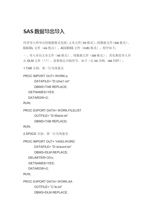
SAS数据导出导入经常导入和导出的数据格式包括:文本文件(txt格式)、纯数据文件(dat格式)、EXCEL文件(xls格式)、ACCESS文件(mdb格式);程序如下:一、导入导出文本文件(txt格式)、纯数据文件(dat格式);其实都是导入导出DLM文件(*.*),需要指定分隔符号。
如下(以txt为例,dat同样):1.TAB分割,第一行为变量名PROC IMPORT OUT= WORK.aDATAFILE= "D:\cha\1.txt"DBMS=TAB REPLACE;GETNAMES=YES;DATAROW=2;RUN;PROC EXPORT DATA= WORK.FILELISTOUTFILE= "D:\filelist.txt"DBMS=TAB REPLACE;RUN;2.SPACE分割,第一行为变量名PROC IMPORT OUT= YANG.WORDDATAFILE= "D:\a\word.txt"DBMS=DLM REPLACE;DELIMITER='20'x;GETNAMES=YES;DATAROW=2;RUN;PROC EXPORT DATA= WORK.AAOUTFILE= "C:\b.txt"DBMS=DLM REPLACE;DELIMITER='20'x;RUN;二、导入导出EXCEL文件(xls格式)程序如下:PROC IMPORT OUT= WORK.ALLWORDDATAFILE= "F:\cc.xls"DBMS=EXCEL REPLACE;SHEET="Sheet1$";GETNAMES=YES;RUN;PROC EXPORT DATA= WORK.AOUTFILE= "D:\export1.xls"DBMS=EXCEL REPLACE;SHEET="nameofsheet";RUN;三、导入导出ACCESS文件(mdb格式)程序如下:PROC IMPORT OUT= WORK.aaDATATABLE= "username"DBMS=ACCESS REPLACE;DATABASE="D:\all\userinfo.mdb";RUN;PROC EXPORT DATA= WORK.AOUTTABLE= "export1"DBMS=ACCESS REPLACE;DATABASE="D:\example.mdb"; *must be an exsited database; RUN;。
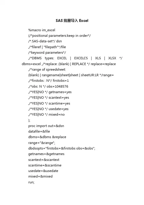
SAS批量导入Excel%macro im_excel(/*positional parameters:keep in order*//*.SAS-data-set*/ dsn,/*fileref | "filepath"*/file/*keyword parameters*/,/*DBMS types: EXCEL | EXCELCS | XLS | XLSX */ dbms=excel ,/*replace: (blank) | REPLACE */ replace=replace ,/*range of spreedsheet:(blank) | rangename|sheet|sheet | sheetUR:LR */range=,/*firstobs : N*/ firstobs=1,/*obs: N */ obs=1048576,/*YES|NO */ getnames=yes,/*YES|NO */ scantext=yes,/*YES|NO */ scantime=yes,/*YES|NO */ usedate=yes,/*YES|NO */ mixed=no);proc import out=&dsndatafile=&filedbms=&dbms &replacerange="&range";dbdsopts="firstobs=&firstobs obs=&obs";getnames=&getnamesscantext=&scantextscantime=&scantimeusedate=&usedatemixed=&mixedrun;%mend im_excel;%macro im_1m1excel(RootPath,FileName,Extension); libname MyExcel Excel "&RootPath.\&Filename..&Extension"; proc sql noprint;select catt(trim(libname),'.',quote(trim(memname)),'n') into: namelist seperated by ' 'from dictionary.tableswhere libname in ('MYEXCEL');quit;%put &namelistdata &FileNameset &namelistrun;%mend im_1m1excel;%macro im_m1mexcel(dir=) ; filename indata pipe "dir &dir /b"; data FileName;length fname $20.;infile indata truncover;input fname $20.;dname=scan(fname,1,".");call symputx(cats('File',_n_),fname); call symputx(cats('ds',_n_),dname); call symputx('NumFile',_n_);run;%do i=1 %to &NumFileproc import out=&&ds&idatafile="&Dir\&&file&i"dbms=excel replace;run;%end;%mend;。
sas使用方法范文SAS(Statistical Analysis System)是一种统计分析软件,广泛应用于数据管理和分析。
它提供了一系列功能强大的工具和处理数据的方法。
下面将介绍SAS的使用方法,包括数据导入、数据处理、数据分析和数据可视化等。
1.数据导入:SAS可以导入多种格式的数据文件,如Excel、CSV和文本文件。
使用SAS的数据步骤(data step),可以将数据导入到SAS数据集中。
以下是一个导入Excel文件的示例代码:```data mydata;infile 'path_to_file\myfile.xlsx'dbms=xlsx replace;sheet='sheet1';getnames=yes;run;```2.数据处理:SAS提供了多种数据处理的方法。
例如,通过数据步骤可以对数据进行清洗、转换和整理。
以下是一些常用的数据处理操作:-选择变量:使用KEEP或DROP语句选择需要的变量。
-变量变换:使用COMPUTE语句创建新变量。
-数据过滤:使用WHERE语句根据条件筛选数据。
-数据合并:使用MERGE语句将多个数据集合并在一起。
3.数据分析:SAS提供了丰富的数据分析功能,可以进行统计分析、建模和预测等操作。
以下是一些常用的数据分析方法:-描述统计:使用PROCMEANS、PROCFREQ和PROCSUMMARY等过程进行数据的描述统计分析。
-方差分析:使用PROCANOVA进行方差分析。
-回归分析:使用PROCREG进行线性回归分析。
-聚类分析:使用PROCFASTCLUS进行聚类分析。
-因子分析:使用PROCFACTOR进行因子分析。
-时间序列分析:使用PROCARIMA进行时间序列分析。
4.数据可视化:SAS提供了多种方法用于数据可视化。
通过使用SAS的图形过程(PROCGPLOT和PROCSGPLOT等),可以绘制各种类型的图表,如柱状图、散点图、折线图和饼图等。
SAS数据的导入、导出及树状图的保存
数据的导入及导出
1数据的导入
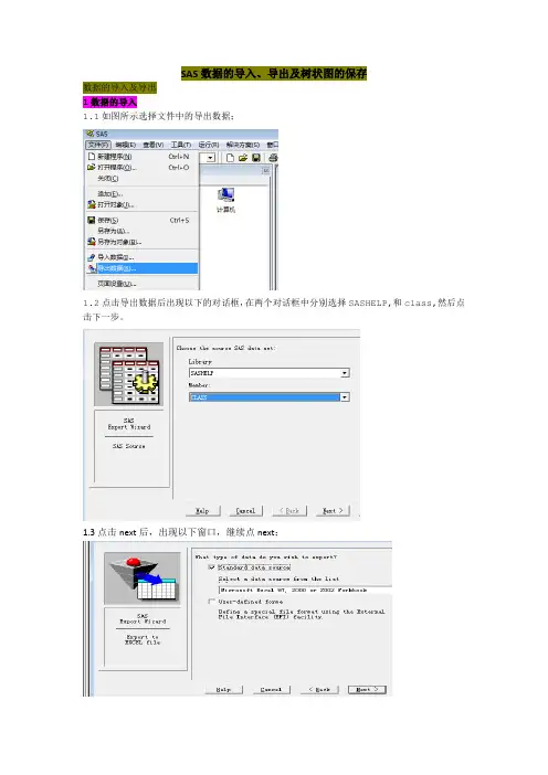
1.1如图所示选择文件中的导出数据;
1.2点击导出数据后出现以下的对话框,在两个对话框中分别选择SASHELP,和class,然后点击下一步。
1.3点击next后,出现以下窗口,继续点next;
1.4然后出现以下对话框,点击browse
1.5然后选中多元数据文件包
1.6然后命名为数据集1,点击保存;
1.7然后点击保存-OK-finish,即完成了数据集的导出
2数据的导入
2.1选择文件-导入数据即出现以下对话框
2.2点击next-browse选中数据集1进行导入
2.3点击打开-ok-next出现以下对话框,将导入的文件命名为paper,选择finish,
3树状图的保存
3.1点击树状图-单击右键-文件-导出图像
3.2点击导出图像-出现下图-命名为树状图保存即可。
SAS使用技巧范文SAS(统计分析系统)是一种常用于统计分析和数据处理的软件工具。
它具有强大的数据管理和分析功能,可以用于处理大规模数据,进行统计建模和预测。
下面是一些SAS使用的技巧,可以帮助您更高效地使用这个软件。
1.数据导入和导出在SAS中,可以使用“数据步骤”(data step)或“导入向导”(import wizard)将数据导入到SAS系统中。
对于非常大的数据集,可以使用“数据步骤”的输入语句来减少内存的使用。
另外,SAS也支持各种数据格式的导入和导出,如CSV、Excel、SPSS等。
2.数据清洗和转换在进行数据分析之前,通常需要先对数据进行清洗和转换。
SAS提供了一系列的数据转换函数和过程,可以通过数据步骤或SAS语句来处理数据。
比如,可以使用“keep”语句来选择感兴趣的变量,使用“drop”语句来删除不需要的变量,使用“rename”语句来重命名变量。
3.数据合并和拆分有时候需要将多个数据集合并在一起,或将一个数据集拆分成多个部分进行分析。
SAS提供了“merge”和“append”过程来合并数据集,可以根据一个或多个共同变量来进行合并。
另外,可以使用“split”和“sample”过程来将一个数据集拆分成多个部分。
4.数据查询和筛选在进行数据分析时,需要根据一定的条件对数据进行查询和筛选。
SAS提供了类似于SQL的语句来完成这些任务。
可以使用“where”子句来筛选数据,使用“subset”函数来选择一部分数据。
另外,还可以使用“proc sql”过程来执行更复杂的查询操作。
5.数据汇总和计算在进行数据分析时,通常需要对数据进行汇总和计算。
SAS提供了一些过程和函数来完成这些任务。
可以使用“proc means”过程来计算变量的均值、标准差等统计量,使用“proc freq”过程来计算变量的频率分布,使用“proc summary”过程来进行更复杂的汇总操作。
6.数据图形化图形化是数据分析的重要环节,可以帮助我们更好地理解数据和发现规律。
数据分析—SAS数据导入导出鉴于市面上SAS基础知识学习资料较多,在这里不过多介绍。
现分享自己在SAS软件学习和使用过程中总结的相关数据导入导出常见问题,与大家分享。
导入csv、xlsx文件(import语句)PROC IMPORT DATAFILE="E:\xxxxxx\export.csv"out=test;run;a)导入的数据如字段名称为中文可能无法展现字段名称(var1/var2…)解决方法-设置变量名为任意值options validvarname=any;PROC IMPORT DATAFILE="E:\xxxxxx\export.csv"out=test;run;b)编码格式问题导致的导入数据乱码获得SAS编码(其实是通过启动时加载配置文件决定的,nls)启动后无法修改。
如尝试通过下面命令设置,会得到警告。
option encoding='utf-8';日志:因此,在导入导出的时候,我们可以指定导入或导出文件的编码。
比如要导入的csv文件为utf-8编码格式,变量名称为中文,可尝试以下代码options validvarname=any;filename nls " E:\xxxxxx\export.csv"ENCODING="utf-8";PROC IMPORT DATAFILE="E:\xxxxxx\export.csv"out=test;run;对应的utf-8编码文件导出代码为:filename export "E:\xxxxxx\export.csv"ENCODING="utf-8";PROC EXPORT DATA= TEST OUTFILE= exportDBMS=csv REPLACE;RUN;1。
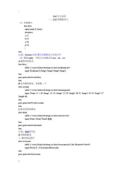
SAS学习总结一、SAS的数据录入(1)直接输入data first;input name $ salary;datalines;a 12b 34c 56d 78;run;注意:datalines的位置以及数据录入后的分号(2)借助infile 可读入文本格式为dat、txt、csvA.最简单的形式data first;infile 'c:\users\lichao\desktop\sas\data\toadjump.dat';input Toadname $ Jump1 Jump2 Jump3 Jump4;run;proc print data=work.first;run;B.有空格的情况,需要数一下data second;infile 'c:\users\lichao\desktop\sas\data\onionring.dat';input Name $ 1-19 Jump1 22-24 Jump2 25-28 Jump3 30-31 Jump4 33-34 Jump5 37 Jump6 40;run;proc print data=work.second;run;C.格式重复的情况data third;infile 'c:\users\lichao\desktop\sas\data\exercise.dat';input Num1 Num2 Num3 @@;run;proc print data=work.third;run;注意:@@的用法D.其他的格式Ⅰ.输出特定的行data icecream;infile 'c:\users\lichao\desktop\sas\data\icecreamsales2.dat' firstobs=3 obs=5;input Flavor $ 1-9 Location Boxessold;run;proc print data=icecream;run;注意:firstobs和obs的位置不要改变,而且两者可以单独使用Ⅱ.有缺失值data class;infile 'c:\users\lichao\desktop\sas\data\allscores.dat' missover;input name $ test1 test2 test3 test4 test5;run;proc print data=class;run;注意:在有缺失值的情况下,如果输出有错误的话就用missoverⅢ.非正常的输入:data third;infile 'c:\users\lichao\desktop\sas\data\pumpkin.dat';input Name $16. num 3. type $2. date $11. (num1 num2 num3 num4 num5) (4.1); run;proc print data=third;run;注意:16. 和3. 、4.1等的表示方法,都是表示宽度,相比较数列数的方法更有效;输入格式相同的话可以加括号把格式写在后面的括号里。
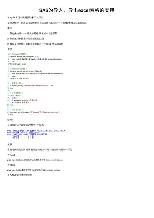
SAS的导⼊、导出excel表格的实现⾸先 SAS 可以使⽤⼿动来导⼊,导出但是这样对于每次操作都需要来⼿动操作,所以就使⽤了 SAS 中的宏来编写代码需求:1. ⾸先是给定excel 的⽂件路径,来⽣成⼀个数据集2. 然后是对数据集中进⾏数据的处理3. 最后是对处理好的数据集导出为⼀个excel 格式的⽂件例⼦:1/* 导⼊excel的数据 */2 %macro import_excel(filepath, out);3 proc import datafile=&filepath out=&out dbms=excel replace;4 run;5 %mend import-excel;67/* 导出excel的数据 */8 %macro export_excel(dataset, filepath);9 proc export data=&dataset file=&filepath dbms=excel replace;10 run;11 %mend export_excel();1213/* 调⽤导⼊宏 */14 %import_excel('C:\Users\ZEK\Desktop\test.xlsx', a);15 run;1617/* 处理数据集 */18 data process;19set a;20if age>14 then desc='已满14岁';21else desc='未满14岁';22 run;2324/* 调⽤导出宏 */25 %export_excel(process, 'C:\Users\ZEK\Desktop\temp.xlsx');26 run;结果:在⽇志窗⼝中会输出这样的⼀个⽇志.注意:在编写代码的时候,最需要注意的是,导⼊和导出的语句是不⼀样的导⼊为:proc import datafile=路径名称out=数据集名称 dbms=excel replace;导出为:proc export data=数据集名称 file=路径名称 dbms=excel replace;千万要注意。
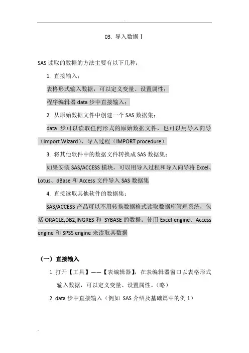
03. 导入数据ⅠSAS读取的数据的方法主要有以下几种:1. 直接输入;表格形式输入数据,可以定义变量、设置属性;程序编辑器data步中直接输入;2. 从原始数据文件中创建一个SAS数据集;data步可以读取任何形式的原始数据文件,也可以用导入向导(Import Wizard)、导入过程(IMPORT procedure)3. 将其他软件中的数据文件转换成SAS数据集;如果安装SAS/ACCESS模块,可以用导入过程和导入向导将Excel、Lotus、dBase和Access文件导入SAS数据集4. 直接读取其他软件的数据集;SAS/ACCESS产品可以不用转换数据格式读取数据库管理系统,包括ORACLE,DB2,INGRES和SYBASE的数据;使用Excel engine、Access engine和SPSS engine来读取其数据(一)直接输入1.打开【工具】——【表编辑器】,在表编辑器窗口以表格形式输入数据,可以定义变量、设置属性。
(略)2.data步中直接输入(例如SAS介绍及基础篇中的例1)(二)用导入向导(Import Wizard)读取文件步骤:1.打开【文件】——【导入数据】,调出导入向导窗口;2.选择要导入的数据类型;3.指定要导入的文件位置,SAS默认第一行存放变量名,从第二行开始存放数据(Options可以改变这种默认选择);4.选择数据集要存放的地址,并为数据集命名;5.(可选)创建一个proc import语句,可以执行它再次导入这个数据。
(三)从外部文件导入数据一、读取空格或分隔符分开的数据语法:data 数据集名;infile ‘文件路径+文件名’ <可选参数>;input变量1 变量2 …;注:infile语句告诉SAS外部数据的存放路径和文件名;示例:data students;infile'c:\MyRawData\Studens.dat' DLM = ',';input Name $ Age Height;注:这是创建临时数据集work.students,若要创建永久数据集,需要指定二级数据集名称。
运用import过程进行SAS数据导入完全实用教程1 单个规范格式文件导入。
1.1 对指定分隔符(’|’,’’,’!’,’ab’等)数据的导入,这里以’!’为例delimiter='!'进行说明:data _null_;file 'c:\temp\pipefile.txt';put"X1!X2!X3!X4";put "11!22!.! ";put "111!.!333!apple";run;proc importdatafile='c:\temp\pipefile.txt'out=work.testdbms=dlmreplace;delimiter='!';GUESSINGROWS=2000;DATAROW=2;getnames=yes;run;注意GUESSINGROWS的值阈为1 到 32761.2 对CSV格式的数据进行导入:data _null_;file 'c:\temp\csvfile.csv';put "Fruit1,Fruit2,Fruit3,Fruit4";put "apple,banana,coconut,date";put "apricot,berry,crabapple,dewberry"; run;proc importdatafile='c:\temp\csvfile.csv'out=work.fruitdbms=csvreplace;run;1.3 对tab分隔数据的导入:data _null_;file 'c:\temp\tabfile.txt';put "cereal" "09"x "eggs" "09"x "bacon";put "muffin" "09"x "berries" "09"x "toast"; run;proc importdatafile='c:\temp\tabfile.txt'out=work.breakfastdbms=tabreplace;getnames=no;run;1.4 对dbf数据库数据进行导入:proc import datafile="/myfiles/mydata.dbf"out=sasuser.mydatadbms=dbfreplace;run;1.5对excel数据进行导入:PROC IMPORT OUT= hospital1DATAFILE= " C:\My Documents\Excel Files\Hospital1.xls "DBMS=EXCEL REPLACE;SHEET="Sheet1$";GETNAMES=YES;MIXED=NO;SCANTEXT=YES;USEDATE=YES;SCANTIME=YES;RUN;1.6对access数据进行导入:PROC IMPORT DBMS=ACCESS TABLE="customers" OUT=sasuser.cust;DATABASE="c:\demo\customers.mdb";UID="bob";PWD="cat";WGDB="c:\winnt\system32\system.mdb"; RUN;proc print data=sasuser.cust;run;1.7 import过程步中,dbms选项汇总:2 导入一个文件夹下的所有文件的数据。
sas数据导⼊终极汇总-之中的⼀个将数据⽂件读⼊SAS ——DATA Step / PROC IMPORT1.将SAS⽂件读⼊SAS——data sasuser.saslin;set "F:\sas1.sas7bdat";run;proc contents data=sasuser.saslin;run;2.将其它形式⽂件导⼊成SAS ——PROC IMPORT / 直接读⼊其它形式⽂件proc import datafile = "c:\data\hsb2.sav" out= work.hsb2;run;proc contents data=hsb2;run;SAS导⼊数据:SAS recognizes the file type to be imported by file extension.对数据长度的限制在⼀些操作环境,SAS假定外部⽂件的纪录对最长为256(⼀⾏数据包含空格等全部字符在内的长度),假设估计读⼊的纪录长度超过256,可在Infile语句中使⽤LRECL=n 这个命令。
读⼊以空格作为分隔符的原始数据假设原始数据的不同变量之间是以⾄少⼀个空格作为分隔符的。
那能够直接採⽤List⽅法将这些数据读⼊SAS。
List Input读数据⾮常⽅便,但也有⾮常多局限性:(1)不能跳过数据;(2)全部的缺失值必须以点取代(3)字符型数据必须是不包括空格的,且长度不能超过8;(4)不能直接读⼊⽇期型等特殊类型的数据。
程序举例:INPUT Name $ Age Height;读⼊按列组织的数据有些原始数据的变量之间没有空格或其它分隔符,因此这种⽂件不能以List形式对⼊SAS。
但若不同变量值的都在每条记录的固定位置处,则能够依照Column 形式读⼊数据。
Colunm读数据⽅法要求全部的数据均为字符型或者标准的数值型(数值中仅包含数字,⼩数点,正负号,或者是E,不包含逗号或⽇期型数据)。
SAS数据整理的16个技巧SAS是一种广泛使用的数据分析和统计软件,而数据整理是数据分析过程中的重要一环。
在SAS中,有很多技巧可以帮助我们有效地进行数据整理和清洗。
下面是16个常用的SAS数据整理技巧。
1.了解数据的结构:在开始进行数据整理之前,我们需要先了解数据的结构,包括数据的类型、变量、变量类型等等。
这样有助于我们制定适当的数据整理策略。
2.导入数据:使用SAS的数据导入功能将数据文件导入到SAS中进行处理。
3.查看数据:使用PROCCONTENTS和PROCPRINT等SAS的过程来查看导入的数据,并了解数据的基本信息。
4.缺失值处理:使用IFTHEN语句来判断和处理数据中的缺失值。
可以选择删除缺失值、替换缺失值、插补缺失值等处理方法。
5.去除重复值:使用PROCSORT和PROCSORTNODUPKEY等SAS过程来去除数据中的重复观测值。
6.数据排序:使用PROCSORT对数据进行排序。
可以根据一个或多个变量进行排序。
7.变量重命名:使用RENAME语句来重命名变量名称。
可以将变量名称改为更直观和易懂的名称。
8.缺失值编码:通过对缺失值进行编码,将缺失值特别标记出来,便于后续数据分析。
9.数据变量类型转换:使用DATA步骤和相关函数将数据变量的类型进行转换。
可以将字符型转换为数值型,反之亦然。
10.缺失值填充:使用PROCMEANS、PROCSUMMARY等过程计算变量的均值、中位数等统计量,然后使用DATA步骤和ARRAY和DO循环等SAS技巧将缺失值进行填充。
11.创建指标变量:通过使用IFTHEN语句基于一些条件来创建指标变量。
例如,可以根据一些变量的取值来创建一个二元指标变量。
12.数据合并:使用PROCAPPEND、SET语句和DATA步骤将多个数据集合并成一个数据集。
13.数据分割:使用DATA步骤和IFTHEN语句将数据集按照一些变量进行拆分,例如将数据按照时间、地区等因素进行分割。
04. 导入数据Ⅱ——Excel文件(一)导入Excel数据文件一、import语句导入语法:proc import datafile=’文件路径+文件名’ OUT=输出数据集名 DBMS=EXCEL REPLACE;<可选参数>;注:(1)REPLACE告诉SAS若“输出数据集”同名文件已经存在,则替换它;(2)可选参数:a. 指定要读取的是哪一个工作表SHEET = 工作表名;b. 若只读取工作表的一部分围RANGE = "工作表名$A1:H10";c. 是否从工作表的第一行读取数据集的列变量名?GETNAMES=YES——是;GETNAMES=NO——否;d. 读取字符和数值混合的数据表时,是否将所有数据转化为字符?MIXED=YES——是;MIXED=NO——否;示例:proc import DATAFILE = 'c:\MyRawData\OnionRing.xls'OUT=sales DBMS=XLS REPLACE;例1 路径“D:\我的文档\My SAS Files\9.3\”下的数据文件exercise.xlsx,容如下:读取工作表test2中从A1到H10的数据,第一行作为数据集的列变量名。
代码:proc import datafile = 'D:\我的文档\My SASFiles\9.3\exercise.xlsx'DBMS=EXCEL OUT = results REPLACE;SHEET = 'tests2';RANGE = '$A1:H10';GETNAMES = YES;run;proc print data = results;title'SAS Data Set Read From Excel File';run;运行结果:二、libname语句读入1. 基本语法用libname语句引用一个Excel文件(“工作簿”),其中的“工作表”作为数据集,数据集名称为:’工作表名$’n语法:libname 引用名‘文件路径+文件名’ <可选参数>;注:(1)访问数据集用:引用名. ’工作表名$’n(2)工作表若有“名称框”(Named Range:单独命名的一部分区域),将单独作为数据集,区别是数据集名没有$示例:libname results 'D:\My SAS Files\exercise.xlsx';proc print data=results.'tests1$'n;例2 路径“D:\我的文档\My SAS Files\9.3\”下的数据文件exercise.xlsx,容如下:读取工作表tests1中的数据。
SAS数据集的导⼊
数据集的导⼊
第⼀步:点选⽂件=>导⼊数据,
第⼀步:
选择导⼊数据⽂件的类型,和导出程序⼀样,选择EXCEL相关格式,然后点击next:
第⼆步:进⼊到“选择导⼊数据⽂件”窗⼝,选择⼀个要导⼊的⽂件:
第三步:进⼊到“选择table”窗⼝,可以选择下拉列表的“1”;
第四步:选择要导⼊的数据⽂件所在的逻辑库及⽂件名称,例如,这⾥选择work临时库和test⽂件名,
第五步:进⼊到Import Wizard窗⼝,给前⾯的导⼊过程产⽣⼀段程序,并提⽰是否储存这个程序,如不想存储则直接单击finish按钮,点击“⼯具”,选择“SAS资源管理器”,点击“WORK”,就可以看到我们导⼊的数据“test".
另⼀种⽅法,可以⾃⼰编写程序,导⼊数据:。
SASSAS DATA Step / Viewtable1.Internal raw data- Datalines or Cards2.External Raw data files- Infile + Input ;SAS DATA Step / PROC IMPORT1.SAS SASdata sasuser.saslin;set "F:\sas1.sas7bdat";run;proc contents data=sasuser.saslin;run;2.SAS PROC IMPORT /proc import datafile = "c:\data\hsb2.sav" out= work.hsb2;run;proc contents data=hsb2;run;SAS SAS recognizes the file type to be imported by file extension.SAS256256Infile LRECL=nListSASList Input12384INPUT Name $ Age Height;ListSAS ColumnColunmEList Column1234INPUT Name $ 1-10 Age 11-13 Height 14-18;$informat w.informat w.dDatew.(1)$CHARw.$HEXw. 16$w.(2)DATEw. ddmmmyy ddmmmyyyyDATETIMEw. ddmmmyy hh:mm:ss.ssDDMMYYw. ddmmyy ddmmyyyyJULIANw. yyddd yyyyddd JuliaMMDDYYw. mmddyy mmddyyyyTIMEw. hh:mm:ss.ss(3)COMMAw.d $HEXw. 16IBw.dPERCENTw.w.dINPUT Name $16. Age 3. +1 Type $1. +1 Date MMDDYY10.(Score1 Score2 Score3 Score4 Score5) (4.1);+n n n@nINPUT ParkName $ 1-22 State $ Year @40 Acreage COMMA9.;BreedMy dog Sam Breed: Rottweiler Vet Bills: $4781SAS RottweilBreed DogBreed2SAS Rottweiler Vet BillBreed: DogBreed203SAS RottweilerBreed:DogBreed 20SASnINPUT City $ State $ / NormalHigh NormalLow #3 RecordHigh RecordLow;Input@@SASINPUT City $ State $ NormalRain MeanDaysRain @@;SASINPUT@SASIFINPUTINPUT Type $ @;INPUT Name $ 9-38 AMTraffic PMTraffic; @ & @@ (1)(2) @SAS@@INFILE1FIRSTOBS=n : n2OBS=n n3INPUTSASINPUTSASMISSOVERTRUNCOVERcolumnTRUNCOVER SASDATAINFILE DLM= DSD1The DLM= optionTab2The DSD optionSASIMPORTIMPORT1234SAS56-set;SASDLM IMPORT DBMS=optionSAS REPLACE-set DBMS=identifier REPLACE;IMPORTIMPORT GETNAMES=NOIMPORTDILIMITER=statementPRO-setDBMS=DLM REPLACE;GETNAMES=NO;-RUN;IMPORT PC-setDBMS=identifier REPLACE;SASPROC CONTENTS DATA=data-set;CONTENTS SAS121.cars_novname.csvAcura,MDX,SUV,Asia,All,"$36,945 ","$33,337 ",3.5,6,265,17,23,4451,106,189 Acura,RSX Type S 2dr,Sedan,Asia,Front,"$23,820 ","$21,761",2,4,200,24,31,2778,101,172Acura,TSX 4dr,Sedan,Asia,Front,"$26,990 ","$24,647 ",2.4,4,200,22,29,3230,105,183 Acura,TL 4dr,Sedan,Asia,Front,"$33,195 ","$30,299 ",3.2,6,270,20,28,3575,108,186 Acura,3.5 RL 4dr,Sedan,Asia,Front,"$43,755 ","$39,014",3.5,6,225,18,24,3880,115,197proc import datafile="cars_novname.csv" out=mydata dbms=csv replace;getnames=no;run;proc contents data=mydata;run;SAS creates default variable names as VAR1-VARn when variables names are not present in the raw data file.2.proc import datafile="cars.txt" out=mydata dbms=tab replace;getnames=no;run;3.libname dis "c:\dissertation";proc import datafile="cars.txt" out=dis.mydata dbms=dlm replace;delimiter='09'x;getnames=yes;run;3.proc import datafile="cars_sp.txt" out=mydata dbms=dlm replace;getnames=no;run;4.Other kinds of delimitersYou can use delimiter= on the infile statement to tell SAS what delimiter you are using to separate variables in your raw data file. For example, below we have a raw data file that uses exclamation points ! to separate the variables in the file.22!2930!409917!3350!474922!2640!379920!3250!481615!4080!7827The example below shows how to read this file by using delimiter='!' on the infile statement.DATA cars;INFILE 'readdel1.txt' DELIMITER='!' ;INPUT mpg weight price;RUN;PROC PRINT DATA=cars;RUN;As you can see in the output below, the data was read properly.OBS MPG WEIGHT PRICE1 22 2930 40992 17 3350 47493 22 2640 37994 20 3250 48165 15 4080 7827It is possible to use multiple delimiters. The example file below uses either exclamation points or plus signs as delimiters.22!2930!409917+3350+474922!2640!379920+3250+481615+4080!7827By using delimiter='!+' on the infile statement, SAS will recognize both of these as valid delimiters.DATA cars;INFILE 'readdel2.txt' DELIMITER='!+' ;INPUT mpg weight price;RUN;PROC PRINT DATA=cars;RUN;As you can see in the output below, the data was read properly.OBS MPG WEIGHT PRICE1 22 2930 40992 17 3350 47493 22 2640 37994 20 3250 48165 15 4080 7827importProc import does not know the formats for your variables, but it is able to guess the format based on what the beginning of your dataset looks like. Most of the time, this guess is fine. But if the length of a variable differs from beginning to end of your file, you might end up with some truncated values.-Infile optionsFor more complicated file layouts, refer to the infile options described below.DLM=The dlm= option can be used to specify the delimiter that separates the variables in your raw data file. For example, dlm=','indicates a comma is the delimiter (e.g., a commaseparated file, .csv file). Or, dlm='09'x indicates that tabs are used to separate your variables (e.g., a tab separated file).DSDThe dsd option has 2 functions. First, it recognizes two consecutive delimiters as a missing value. For example, if your file contained the line 20,30,,50 SAS will treat this as 20 30 50 but with the the dsd option SAS will treat it as 20 30 . 50 , which is probably what you intended. Second, it allows you to include the delimiter within quoted strings. For example, you would want to use the dsd option if you had a comma separated file and your data included values like "George Bush, Jr.". With the dsd option, SAS will recognize that the comma in "George Bush, Jr." is part of the name, and not a separator indicating a new variable.FIRSTOBS=This option tells SAS what on what line you want it to start reading your raw data file. If the first record(s) contains header information such as variable names, then setfirstobs=n where n is the record number where the data actually begin. For example, if you are reading a comma separated file or a tab separated file that has the variable names on the first line, then use firstobs=2 to tell SAS to begin reading at the second line (so it will ignore the first line with the names of the variables).MISSOVERThis option prevents SAS from going to a new input line if it does not find values for all of the variables in the current line of data. For example, you may be reading a space delimited file and that is supposed to have 10 values per line, but one of the line had only 9 values. Without the missover option, SAS will look for the 10th value on the next line of data. If your data is supposed to only have one observation for each line of raw data, then this could cause errors throughout the rest of your data file. If you have araw data file that has one record per line, this option is a prudent method of trying to keep such errors from cascading through the rest of your data file.OBS=Indicates which line in your raw data file should be treated as the last record to be read by SAS. This is a good option to use for testing your program. For example, you might use obs=100 to just read in the first 100 lines of data while you are testing your program. When you want to read the entire file, you can remove the obs= option entirely.A typical infile statement for reading a comma delimited file that contains the variable names in the first line of data would be:INFILE "test.txt" DLM=',' DSD MISSOVER FIRSTOBS=2 ;DATA cars2;length make $ 20 ;INFILE 'readdsd.txt' DELIMITER=',' DSD ;INPUT make mpg weight price;RUN;PROC PRINT DATA=cars2;RUN;48,'Bill Clinton',21050,'George Bush, Jr.',180DATA guys2;length name $ 20 ;INFILE 'readdsd2.txt' DELIMITER=',' DSD ;INPUT age name weight ;RUN;PROC PRINT DATA=guys2;RUN;DATA cars2;length nf 8;INFILE 'F:\cars1.csv' DELIMITER=',' dsd MISSOVER firstobs=2 ;INPUT nf zh hh xb cs IHA fj;RUN;PROC PRINT DATA=cars2;RUN;FTPread raw data via FTP in SAS?SAS has the ability to read raw data directly from FTP servers. Normally, you would use FTP to download the data to your local computer and then use SAS to read the data stored on your local computer. SAS allows you to bypass the FTP step and read the data directly from the other computer via FTP without the intermediate step of downloading the raw data file to your computer. Of course, this assumes that you can reach the computer via the internet at the time you run your SAS program. The program below illustrates how to do this. After the filename in you put ftp to tell SAS to access the data via FTP. After that, you supply the name of the file (in this case 'gpa.txt'. lrecl= is used to specify the width of your data. Be sure to choose a value that is at least as wide as your widest record. cd= is used to specify the directory from where the file is stored. host= is used to specify the name of the site to which you want to FTP. user= is used toprovide your userid (or anonymous if connecting via anonymous FTP). pass= is used to supply your password (or your email address if connecting via anonymous FTP).FILENAME in FTP 'gpa.txt' LRECL=80CD='/local2/samples/sas/ats/'HOST=''USER='joebruin'PASS='yourpassword' ;DATA gpa ;INFILE in ;INPUT gpa hsm hss hse satm satv gender ;RUN;PROC PRINT DATA=gpa(obs=10) ;RUN;quarter1.dat1 120321 1236 154669 2113261 326264 1326 163354 3126651 420698 1327 142336 4226851 211368 1236 156327 6552371 378596 1429 145678 366578quarter2.dat2 140362 1436 114641 3624152 157956 1327 124869 3452152 215547 1472 165578 4125672 204782 1495 150479 3644742 232571 1345 135467 332567quarter3.dat3 140357 1339 142693 2058813 149964 1420 152367 2237953 159852 1479 160001 2548743 139957 1527 163567 2630883 150047 1602 175561 277552quarter4.dat4 479574 1367 155997 361344 496207 1459 140396 359414 501156 1598 135489 396404 532982 1601 143269 386954 563222 1625 147889 39556filename year ('d:\quarter1.dat' 'd:\quarter2.dat' 'd:\quarter3.dat' 'd:\quarter4.dat'); data temp;infile year;input quarter sales tax expenses payroll;run;proc print data = temp;run;excelReading an Excel file into SASSuppose that you have an Excel spreadsheet called auto.xls. The data for this spreadsheet are shown below.MAKE MPG WEIGHT PRICEAMC Concord 22 2930 4099AMC Pacer 17 3350 4749AMC Spirit 22 2640 3799Buick Century 20 3250 4816Buick Electra 15 4080 7827Using the Import Wizard is an easy way to import data into SAS. The Import Wizard can be found on the drop down file menu. Although the Import Wizard is easy it can be time consuming if used repeatedly. The very last screen of the Import Wizard gives you the option to save the statements SAS uses to import the data so that they can be used again. The following is an example that uses common options and also shows that the file was imported correctly.PROC IMPORT OUT= WORK.auto1DATAFILE= "C:\auto.xls"DBMS=EXCEL REPLACE;SHEET="auto1";GETNAMES=YES;MIXED=YES;USEDATE=YES;SCANTIME=YES;RUN;proc print data=auto1;run;Obs MAKE MPG WEIGHT PRICE1 AMC Concord 22 2930 40992 AMC Pacer 17 3350 47493 Amc Spirit 22 2640 37994 Buick Century 20 3250 48165 Buick Electra 15 4080 7827First we use the out= statement to tell SAS where to store the data once they are imported.Next the datafile= statement tells SAS where to find the file we want to import.The dbms= statement is used to identify the type of file being imported. This statement is redundant if the file you want to import already has an appropriate file extension, for example *.xls.The replace statement will overwrite an existing file.To specify which sheet SAS should import use the sheet="sheetname" statement. The default is for SAS to read the first sheet. Note that sheet names can only be 31 characters long.The getnames=yes is the default setting and SAS will automatically use the first row of data as variable names. If the first row of your sheet does not contain variable names use the getnames=no.SAS uses the first eight rows of data to determine whether the variable should be read as character or numeric. The default setting mixed=no assumes that each variable is either all character or all numeric. If you have a variable with both character and numeric values or a variable with missing values use mixed=yes statement to be sure SAS will read it correctly.Conveniently SAS reads date, time and datetime formats. The usedate=yes is the default statement and SAS will read date or time formatted data as a date. When usedate=no SAS will read date and time formatted data with a datetime format. Keep the default statement scantime=yes to read in time formatted data as long as the variable does not also contain a date format.Example 1: Making a permanent data fileWhat if you want the SAS data set created from proc import to be permanent? The answer is to use libname statement. Let's say that we have an Excel file called auto.xls in directory "d:\temp" and we want to convert it into a SAS data file (call it myauto) and put it into the directory "c:\dissertation". Here is what we can do.libname dis "c:\dissertation";proc import datafile="d:\temp\auto.xls" out=dis.myauto replace;run;Example 2: Reading in a specific sheetSometimes you may only want to read a particular sheet from an Excel file instead of the entire Excel file. Let's say that we have a two-sheet Excel file called auto2.xls. The example below shows how to use the option sheet=sheetname to read the second sheet called page2 in it.proc import datafile="auto2.xls" out=auto1 replace;sheet="page2";run;Example 3: Reading a file without variable namesWhat if the variables in your Excel file do not have variable names? The answer here is to use the statement getnames=no in proc import. Here is an example showing how to do this.proc import datafile="a:\faq\auto.xls" out=auto replace;getnames=no;run;Writing Excel files out from SASIt is very easy to write out an Excel file using proc export in SAS version 8. Consider the following sample data file below.Obs MAKE MPG WEIGHT PRICE1 AMC 22 2930 40992 AMC 17 3350 47493 AMC 22 2640 37994 Buick 20 3250 48165 Buick 15 4080 7827Here is a sample program that writes out an Excel file called mydata.xls into the directory "c:\dissertation".proc export data=mydata outfile='c:\dissertation\mydata.xls' replace; run;SAS1.data web;length site $41;input age site $ hits;datalines;12 /default.htm 123456130 /index.htm 97654254 /department/index.htm 987654;proc print;run;Obs site age hits1 /default.htm 12 1234562 /index.htm 130 976543 /department/index.htm 254 987654data web;input age site & $41. hits;datalines;12 /default.htm 123456130 /index.htm 97654254 /department/index.htm 987654;proc print;Obs age site hits1 12 /default.htm 1234562 130 /index.htm 976543 254 /department/index.htm 9876542.data fruit;infile 'C:\messy.txt' delimiter = ' ' dsd;length fruit $22;input zip fruit $ pounds;proc print;run;Obs fruit zip pounds1 apples, grapes kiwi 10034 1234562 oranges 92626 976543 pears apple 25414 987654data fruit;input zip fruit & $22. pounds;datalines;10034 apples, grapes kiwi 12345692626 oranges 9765425414 pears apple 987654;proc print;Obs zip fruit pounds1 10034 apples, grapes kiwi 1234562 92626 oranges 976543 25414 pears apple 987654read a SAS data file when I don't have its format libraryIf you try to use a SAS data file that has permanent formats but you don't have the format library, you will get errors like this.ERROR: The format $MAKEF was not found or could not be loaded.ERROR: The format FORGNF was not found or could not be loaded.Without the format library, SAS will not permit you to do anything with the data file. However, if you use options nofmterr; at the top of your program, SAS will go ahead and process the file despite the fact that it does not have the format library. You will not be able to see the formatted values for your variables, but you will be able to process your data file. Here is an example.OPTIONS nofmterr;libname in "c:\";PROC FREQ DATA=in.auto;TABLES foreign make;RUN;The following program creates exactly the same file, but is a more efficient program because SAS only reads the desired variables.DATA auto2;SET auto (KEEP = make mpg price);RUN;The drop data step option works in a similar way.DATA AUTO2;SET auto (DROP = rep78 hdroom trunk weight length turn displ gratio foreign);RUN;proc compare base = person1 compare = person2 brief; by id;id id;run;。