2001-Traffic and residue cover effects on infiltration

第29卷第8期2009年8月环　境　科　学　学　报　A c t a S c i e n t i a e C i r c u m s t a n t i a eV o l .29,N o .8A u g .,2009基金项目:江苏省交通科技计划重大项目(N o .T Z 0761-010)S u p p o r t e db yt h e T r a n s p o r t a t i o nS c i e n c e a n dT e c h n o l o g y p l a n o f J i a n g s u (N o .T Z 0761-010)作者简介:傅大放(1966—),男,教授;＊通讯作者(责任作者),E -m a i l :f d f @s e u .e d u .c nB i o g r a p h y :F UD a f a n g (1966—),m a l e ,p r o f e s s o r ;＊C o r r e s p o n d i n ga u t h o r ,E -m a i l :f d f @s e u .e d u .c n傅大放,石峻青,李贺.2009.高速公路雨水径流重金属污染初期效应[J ].环境科学学报,29(8):1672-1677F u DF ,S h i J Q ,L i H .2009.F i r s t f l u s ha n a l y s i so f h e a v y m e t a l s i ne x p r e s s w a ys t o r m w a t e r r u n o f f [J ].A c t aS c i e n t i a eC i r c u m s t a n t i a e ,29(8):1672-1677高速公路雨水径流重金属污染初期效应傅大放＊,石峻青,李贺东南大学市政工程系,南京210096收稿日期:2008-10-10 修回日期:2009-02-26 录用日期:2009-06-03摘要:通过对8场降雨高速公路路面雨水径流中溶解态和颗粒态C d 、C u 、P b 和Z n 4种重金属进行现场取样检测,在定性分析径流重金属污染初期效应存现的基础上,定量分析了重金属污染初期效应的显著程度,并探讨了降雨特征对径流重金属污染初期效应的影响.无因次累积负荷分数-累积体积分数曲线分析结果表明,大多数降雨事件中总重金属存在较显著的初期效应,除溶解态P b 不具有初期效应外,其余溶解态与颗粒态重金属均存在较显著的初期效应.少数降雨事件的径流在中后期存在二次冲刷效应.初期冲刷比值分析结果表明,拦截并处理径流初期25%流量(径流的体积分数,下同)可去除整个降雨事件中所排放的35%～39%(质量分数,下同)的重金属污染负荷.总重金属初期效应的显著程度顺序如下:C d >C u >Z n >P b ;溶解态重金属初期效应的显著程度顺序如下:C d >Z n >C u >P b ;颗粒态重金属初期效应的显著程度顺序为:C u >C d >P b >Z n .重金属初期冲刷比值与降雨特征相关性分析表明,平均降雨强度对径流重金属污染负荷初期效应的影响显著,降雨历时、降雨量、前期晴天数和产流时间对径流重金属污染负荷初期效应的影响较小.关键词:路面径流;重金属;初期效应文章编号:0253-2468(2009)08-1672-06 中图分类号:X 52 文献标识码:AF i r s t f l u s ha n a l y s i s o f h e a v y m e t a l s i ne x p r e s s w a y s t o r m w a t e r r u n o f fF UD a f a n g ＊,S H I J u n q i n g ,L I H eD e p a r t m e n t o f M u n i c i p a lE n g i n e e r i n g ,S o u t h e a s t U n i v e r s i t y ,N a n j i n g 210096R e c e i v e d 10O c t o b e r 2008; r e c e i v e di nr e v i s e d f o r m 26F e b r u a r y 2009; a c c e p t e d 3J u n e 2009A b s t r a c t :T h e f o c u s o f t h i s s t u d y w a s t h e h e a v y m e t a l s ,C u ,Z n ,P b a n dC d ,c o m m o n l y f o u n di n l a n d u s e df o r t r a n s p o r t a t i o n .D i s s o l v e d a n d p a r t i c u l a t e -b o u n df r a c t i o nc o n c e n t r a t i o n s o f t h e s e m e t a l s w e r em e a s u r e d d u r i n g 8r a i n f a l l -r u n o f f e v e n t s o nar e p r e s e n t a t i v e e x p r e s s w a y p a v e m e n t i nN a n j i n g .O nt h e b a s i s o f a q u a l i t a t i v e e v a l u a t i o no f f l u s h i n g ,t h e f i r s t f l u s h o f h e a v y m e t a l s w a s q u a n t i t a t i v e l y a n a l y z e d ,a n d t h e i n f l u e n c e s o f h y d r o l o g i c c h a r a c t e r i s t i c s o n t h ef i r s t f l u s ha r e d i s c u s s e d .T h e r e s u l t s o f t h e a n a l y s i s o f d i m e n s i o n l e s s n o r m a l i z e dc u m u l a t i v e m a s s a n d v o l u m e c u r v e s i n d i c a t e dt h a t t o t a l ,d i s s o l v e d a n d p a r t i c u l a t e -b o u n d m e t a l s ,e x c e p t d i s s o l v e dP b ,e x h i b i t e da p r o n o u n c e df i r s t f l u s hi nm o s t e v e n t s .T h es e c o n df l u s ha l s oe x h i b i t e di ns o m e e v e n t s .T h e i n i t i a l f l u s hr a t i o d e m o n s t r a t e dt h a t a b o u t 35%t o 39%o f h e a v y m e t a l s c o u l db e r e m o v e df r o mr o a dr u n o f f b y i n t e r c e p t i n g a n d t r e a t i n g t h e i n i t i a l 25%o f t h er u n o f f w a t e r .T h e s e q u e n c e o f s t r e n g t h o f t h e f i r s t f l u s ho f t o t a l m e t a l s w a s :C d >C u >Z n >P b ;f o r t h e d i s s o l v e dm e t a l s :C d >Z n >C u >P b ;a n d f o r t h ep a r t i c u l a t e -b o u n d m e t a l s :C u >C d >P b >Z n .C o r r e l a t i o n a n a l y s i s s u g g e s t e d t h a t t h e i n f l u e n c e o f m e a n r a i n f a l l i n t e n s i t y o n t h e f i r s t f l u s h o f m e t a l s w a s s i g n i f i c a n t ,b u t t h e r e w a s n o s i g n i f i c a n t i n f l u e n c e c a u s e db yo t h e r r a i n f a l l f a c t o r s .K e y w o r d s :r o a d r u n o f f ;h e a v y m e t a l s ;f i r s t f l u s h1　引言(I n t r o d u c t i o n )路面雨水径流中含有大量的重金属污染物(S a n s a l o n ea n dB u c h b e r g e r ,1997;D r a p p e re t a l .,2000),其形态可分为溶解态(<0.45μm )和颗粒态(>0.45μm )两种.溶解态重金属具有较强的生物可给性,易被水生生物吸收(Y o u s e f e t a l .,1985),可通过食物链等途径进入人体并富集,达到一定浓度后将对人体产生毒害作用;而颗粒态重金属同样可以持久地存在于水体沉淀物中,在一定条件下转变为溶解态进入水环境中(D e a ne t a l .,2005).如果初期径流携带了整个径流过程中产生的大部分污染负荷,则称此现象为初期效应(F i r s t F l u s h )(S a n s a l o n ea n dB u c h b e r g e r ,1997;D r a p p e r e t a l .,2000;L e e e t a l .,2002;D e l e t i c ,1998;B a r r e t t e t a l .,1998).该效应存在与否及其存在程度,与城DOI :10.13671/j .hjkxxb .2009.08.0208期傅大放等:高速公路雨水径流重金属污染初期效应市面源污染控制设施的规模及投资直接相关,因而具有重要的研究价值.H a r r i s i o n和W i l s o n(1985)的监测结果表明,大部分降雨事件中前1h的径流含带了50%的总C d、C u、P b和Z n的污染负荷;H e w i t t和R a s h e d(1992)在英格兰某农村地区的研究表明,溶解态P b、C u和C d具有初期效应;S a n s a l o n e和B u c h b e r g e r(1997)对美国辛辛那提城市道路路面径流研究表明溶解态C u和Z n具有初期效应,而颗粒态重金属的初期效应不显著;F l i n t和D a v i s(2007)对美国马里兰州一处郊区公路所监测的降雨事件中,分别有21%、13%和14%降雨事件的前25%径流量含带了超过50%总C u、P b和Z n污染负荷.若干不同的标准使各文献所报道的初期效应的可比性大大降低.本研究通过对高速公路路面雨水径流重金属进行了现场监测,分析了重金属污染初期效应及其影响因素,为路面径流重金属污染的源头控制及其后续处理积累相关资料和依据.2　研究方法(M e t h o d s)2.1　采样地点本研究选取南京机场高速公路禄口令桥段进行采样监测.路面径流经落水管汇集排放,所采样品为落水管出流.采样点道路特征见表1.表1　取样点特征T a b l e1　T h e c h a r a c t e r i s t i c s o f t h e m o n i t o r e d e x p r e s s w a y道路特征汇水面积/m2路面材料车道数日均交通量/(辆·d-1)周围用地类型禄口高架桥960沥青双向4车道22000居住/交通/耕地2.2　采样方法对整场降雨事件采用人工取样,可较完整地反映重金属的污染特征.径流形成的前30m i n,用聚乙烯瓶每隔3～5m i n取样1次;在径流形成的30～60m i n期间,每隔10～15m i n取样1次;此后每隔30～120m i n取样1次直至降雨事件结束;取样间隔时间可视降雨历时和径流流量改变,每次取样均为1L.由J S-2型虹吸式雨量计(天津气象仪器厂,天津)同步记录降雨特征,雨量计安装地点与取样点直线距离约500m.2.3　重金属测定径流样品及时送至实验室进行分析.依照美国公共卫生协会(A m e r i c a n P u b l i c H e a l t hA s s o c i a t i o n,A P H A)《水与废水标准分析方法》第20版(C l e s c e r i e t a l.,1998)分别测定C d、C u、P b和Z n4种元素的总浓度和溶解态浓度,两者相减求得颗粒态浓度(B r o w n a n dP e a k e,2006).用浓H N O3和HC l溶液(去离子水与浓H C l以体积比1∶1配置的H C l溶液)的湿式方法消解水样,测重金属的总浓度;通过0.45μm混合纤维微孔滤膜过滤水样,取滤液测重金属的溶解态浓度.C u和Z n采用火焰原子吸收光谱法测定,C d和P b采用石墨炉原子吸收光谱法测定.所有玻璃器皿材料均为高硼酸盐玻璃,使用前均在H N O3溶液(去离子水与浓H N O3以体积比1∶1配置的H N O3溶液)中浸泡24h,消解用酸均为优级纯,混合纤维微孔滤膜使用前在H N O3溶液(去离子水与浓H N O3以体积比1∶499配置的H N O3溶液)中浸泡24h,水为去离子水.2.4　初期效应判定方法初期效应可通过无因次累积重金属污染负荷分数m'(t)和无因次累积径流量体积分数v'(t)判定(S a n s a l o n ea n dB u c h b e r g e r,1997),可分别按式(1)和式(2)计算.m′(t)=m(t)M=∫t0c(t)q(t)d t∫　t　r0c(t)q(t)d t(1)v′(t)=v(t)V=∫t0q(t)d t∫　t　r0q(t)d t(2)式中,M为整个径流期间重金属总量(m g);m(t)为t时刻累积的重金属质量(m g);V为总径流量(L); v(t)为t时刻累积的径流量(L);c(t)为随时间变化的重金属浓度(m g·L-1);q(t)为流量(L·m i n-1);t 为时间(m i n);t r为径流总持续时间(m i n).此方法至少可用3种不同的标准判定是否存在初期效应(S a n s a l o n ea n dB u c h b e r g e r,1997;F l i n t a n d D a v i s,2007):(1)m′(t)≥v′(t)(H e l s e l e t a l., 1979),此标准通常借助无因次累积负荷分数-累积体积分数曲线(m′(t)-v′(t)曲线),以v′(t)为横坐标、m′(t)为纵坐标绘制曲线,当曲线在角平分线的上方时可判定存在初期效应,与角平分线距离越远则初期效应越显著;(2)m′(t)≥0.80,且v′(t)≤1673环 境 科 学 学 报29卷0.20(S t a h r ee t a l .,1990);(3)m ′(t )≥0.50且v ′(t )≤0.25(W a n i e l i s t aa n dY o u s e f ,1993).标准(2)与标准(3)较严格.若定义初期冲刷比值F F n 按式(3)计算,则标准(2)和(3)分别等价于F F 20≥4.0和F F 25≥2.0.F F n =m ′(t )v ′(t )(3)3　结果(R e s u l t s )3.1　降雨特征表2列出了所考查降雨事件的特征.由表2可知,所监测的8场降雨事件差异较大,降雨量变化范围为1.2～14.2m m .其中,2008-03-06雨量较小(≤2.0m m );2008-02-25、2008-03-08和2008-03-21等3场降雨事件的雨量较大(>8.0m m );其余4场降雨事件的雨量中等(>2.0m m 且<8.0m m ).平均降雨强度变化范围是0.004～0.026m m ·m i n -1,产流时间的变化范围为8～118m i n .本研究所监测8场降雨事件对大、中、小强度降雨具有较好的代表性,为研究结果的可靠性提供了保证.表2　监测降雨事件的特征T a b l e 2　C h a r a c t e r i s t i c s o f t h e m o n i t o r e d s t o r m e v e n t s编号事件日期降雨历时/m i n 降雨量/m m 平均降雨强度/(m m ·m i n -1)前期晴天数/h产流时间/m i n12008-02-255908.30.014645.89022008-03-063181.20.004237.011832008-03-086208.30.01343.52442008-03-2191414.20.016105.6852008-03-294474.40.010202.12762008-04-051633.00.018183.82672008-04-152446.40.026186.98382008-04-207017.70.0119.0133.2　初期效应的存现受客观条件的限制,本研究未能实测路面降雨径流流量,但采样时记录了降雨开始和径流形成的时间,进而消除了路面径流和降雨之间的滞后性.此外,本研究对象为沥青路面,由于沥青路面在降雨时段内渗量与蒸发量很少,可以忽略不计.因此,以降雨量代替路面径流量q (t )计算累积体积分数v '(t ),并以v ′(t )为横坐标,对应累积重金属负荷分数m ′(t )为纵坐标,绘制C d 、C u 、P b 和Z n 4种元素的总重金属、溶解态重金属和颗粒态重金属的m ′(t )-v ′(t )曲线(见图1).16748期傅大放等:高速公路雨水径流重金属污染初期效应图1　重金属累积负荷分数-累积体积分数曲线[m ′(t )-v ′(t )曲线]F i g .1　R e l a t i o n s h i pb e t w e e nd i m e n s i o n l e s s n o r m a l i z e dc u m u l a t i v e m a s s a n dv o l u m e o f h e a v ym e t a l s 由图1可见,8场降雨事件中,大部分降雨事件径流初期的总C d 、总C u 、总P b 和总Z n 的m ′(t )-v ′(t )曲线均位于角平分线上方.根据前述判定标准(1)可知,大多数降雨事件总重金属存在较显著的初期效应.溶解态C d 、C u 和Z n 与颗粒态C d 、C u 、P b 和Z n 的冲刷特性与总重金属类似,大部分降雨事件中径流初期的m ′(t )-v ′(t )曲线位于角平分线上方,存在较显著的初期效应.3.3　初期冲刷比值F F25图2　F F 25盒状分布图F i g .2　B o x d i s t r i b u t i o nc h a r t s f o r F F 25通过m ′(t )-v ′(t )曲线可以直观地分析径流重金属污染负荷的初期效应存在与否,但这只能定性描述初期效应,而初期冲刷比值F F n 则可以定量研究径流重金属污染负荷初期效应的显著程度.图2中的柱状图显示了本研究所监测降雨事件路面径流初期累积25%径流量时所含带的C d 、C u 、P b 和Z n 4种元素的总重金属、溶解态重金属和颗粒态重金属污染负荷比率的F F 25值的分布情况.由图2可知,若采用较严格的标准(3)判定,仅有1场降雨事件的总C u ,2场降雨事件的溶解态Z n 和3场降雨事件的溶解态C d 存在初期效应.但除溶解态P b 外,大部分降雨事件的F F 25值大于1.0,即径流初期25%流量中仍含带多于25%的重金属污染负荷.通过比较F F 25值的平均值可以确定各元素的初期效应显著程度.结果表明,总重金属初期效应的显著程度顺序如下:总C d >总C u >总Z n >总P b ;溶解态重金属初期效应的显著程度顺序如下:溶解态C d >溶解态Z n >溶解态C u >溶解态P b ;颗粒态重金属初期效应的显著程度顺序如下:颗粒态C u >颗粒态C d >颗粒态P b >颗粒态Z n .4　讨论(D i s c u s s i o n )4.1　初期效应的显著程度根据4种总重金属F F 25值的平均值估算,拦截并处理径流初期25%流量可去除整个事件中所排1675环 境 科 学 学 报29卷放的35%～39%的总重金属污染负荷.甘华阳等(2007)对广州3条公路研究表明,拦截并处理径流初期20%～30%流量可去除整个事件中所排放的50%～60%的总重金属污染负荷.与本研究相比,广州地处南方地区,降雨强度较大,雨水对路面污染的冲刷作用更明显,故径流重金属污染初期效应更显著.已有研究表明,典型降雨事件中溶解态污染物的初期效应比颗粒态污染物更为普遍(S a n s a l o n e a n d B u c h b e r g e r,1997),而径流中大部分P b主要以颗粒态存在,C d、C u和Z n的溶解态比例均高于P b (S a n s a l o n e e t a l.,1996;S a n s a l o n e a n d B u c h b e r g e r, 1997;R e v i t t a n dM o r r i s i o n,1987),故总C d、C u和Z n的初期效应比总P b显著.溶解态重金属的冲刷过程与溶解和冲刷两个过程相关,溶解赋存分配动力学的主要控制因素有路面渗透速率、悬浮颗粒比率、溶解性有机碳(D i s s o l v e d O r g a n i c C a r b o n, D O C)、传导性总溶解固体(T o t a l D i s s o l v e dS o l i d, T D S)和配合体(有机和无机)含量等(D e a ne t a l., 2005),上述控制因素与降雨特征的共同作用决定径流溶解态重金属的冲刷特性.颗粒态重金属与总重金属和溶解态重金属初期效应显著程度顺序差别较大,由此可见不同降雨事件中颗粒态重金属冲刷特性变化程度更大,这主要因为颗粒态污染物的冲刷特性在很大程度上受到降雨特性的影响,冲刷过程更为复杂(S a n s a l o n e a n d B u c h b e r g e r,1997).本研究所监测降雨事件中C d和Z n的溶解态初期效应较颗粒态显著,与前述结论一致.而C u和P b的溶解态初期效应则弱于颗粒态.结合图1与图2可知,8场降雨事件中仅2008-04-15一场降雨中颗粒态C u的初期效应明显强于溶解态C u,其余降雨事件中溶解态C u和颗粒态C u的初期效应显著程度相当.径流中P b绝大部分以颗粒态形式存在,溶解态含量很低且随时间波动较大,不具有规律性,故不存在初期效应.4.2　初期效应的影响因素本研究仅以南京机场高速禄口令桥段为对象,路面材料、用地类型、交通量、大气沉降和路面清扫方式等径流水质影响因素较稳定,故表3列出由S P S S11.5统计软件计算出的径流重金属初期冲刷比值F F25与降雨特征之间的P e a r s o n相关系数,评价各降雨特征对径流重金属污染负荷初期效应的影响.由表3可知,平均降雨强度与初期冲刷比值F F25均呈正相关性.平均降雨强度与溶解态C d和溶解态Z nF F25的相关系数较小(分别为0.242和0.294),但其余相关系数变化范围为0.636～0.869,与总C u和颗粒态C uF F25的相关系数分别达到0.862和0.869,在0.01水平上显著相关;与总C d的相关系数为0.727,两者在0.05水平上显著相关.由此可见,平均降雨强度对径流重金属污染负荷初期效应的影响显著,降雨历时、降雨量、前期晴天数和产流时间与初期冲刷比值F F25的P e a r s o n相关系数的变化范围分别为-0.374～0.235、-0.211～0.560、-0.568～0.221、-0.543～0.311和-0.630～0.308,说明这些降雨特征对径流重金属污染负荷初期效应的影响较小.表3　F F25与降雨特征的P e a r s o n相关系数T a b l e3　R e l a t e dc o e f f i c i e n t s b e t w e e n F F25a n d c h a r a c t e r i s t i c s o f t h e m o n i t o r e d s t o r m e v e n t s降雨特征F F25总C d总C u总P b总Z n溶解态C d溶解态C u溶解态Z n颗粒态C d颗粒态C u颗粒态P b颗粒态Z n降雨历时0.089-0.129-0.2040.117-0.158-0.070-0.3740.072-0.202-0.1830.235降雨量0.4670.3170.1440.462-0.0070.288-0.2110.4000.2350.1600.560平均降雨强度0.727＊0.862＊＊0.6790.7010.2420.6700.2940.6360.869＊＊0.6590.692前期晴天数-0.482-0.246-0.539-0.4410.311-0.323-0.150-0.543-0.202-0.526-0.392产流时间-0.506-0.011-0.557-0.4760.3080.120-0.029-0.6300.029-0.560-0.586 注:＊p<0.05,＊＊p<0.014.3　二次冲刷效应2008-03-21降雨事件中溶解态C u与2008-04-20降雨事件中溶解态C d和溶解态Z n,在径流中后期的一段时间内污染负荷增加较快,m′(t)-v′(t)曲线的斜率较大且位于角平分线以下,这可能出现了二次冲刷现象(S e c o n d F l u s h),即大部分污染负荷16768期傅大放等:高速公路雨水径流重金属污染初期效应存在于径流中后期某一时间段内(F l i n t a n dD a v i s, 2007),这与降雨特性密切相关.F l i n t和D a v i s (2007)在前述初期效应探讨的基础上,同样发现分别在25%、27%和18%的降雨事件中后期某阶段25%径流携带C u、Z n和P b负荷超过初期25%径流,存在二次冲刷.此现象与初期效应类似,对于径流污染控制的最佳管理措施(B e s t M a n a g e m e n t P r a c t i c e s,B M P s)具有重要的理论指导意义,尚需进一步研究.5　结论(C o n c l u s i o n s)1)大多数降雨事件总重金属存在较显著的初期效应,除溶解态P b不具有初期效应外,其余溶解态与颗粒态重金属也存在较显著的初期效应.少数降雨事件径流中后期存在二次冲刷效应.2)拦截并处理径流初期25%流量可去除整个事件中所排放的35%～39%的重金属污染负荷.总重金属初期效应的显著程度顺序如下:总C d>总C u>总Z n>总P b;溶解态重金属初期效应的显著程度顺序如下:溶解态C d>溶解态Z n>溶解态C u >溶解态P b;颗粒态重金属初期效应的显著程度顺序如下:颗粒态C u>颗粒态C d>颗粒态P b>颗粒态Z n.3)平均降雨强度对径流重金属污染负荷初期效应的影响显著,降雨历时、降雨量、前期晴天数和产流时间对径流重金属污染负荷初期效应的影响较小.责任作者简介:傅大放(1966—),男,博士,教授,主要从事交通环境保护.E-m a i l:f d f@s e u.e d u.c n.参考文献(R e f e r e n c e s):B a r r e t t M E,I r i s hLB,M a l i n aJ F,e t a l.1998.C h a r a c t e r i z a t i o no fh i g h w a y r u n o f f i n A u s t i n,T e x a s,A r e a[J].J o u r n a l o fE n v i r o n m e n t a l E n g i n e e r i n g,124(2):131—137B r o w n J N,P e a k eBM.2006.S o u r c e so f h e a v y m e t a l s a n dp o l y c y c l i ca r o m a t i c h y d r o c a rb o n s i nu r b a n s t o r m w a t e r r u n o f f[J].Sc i e n c e o f t h eT o t a l E n v i r o n m e n t,359(1-3):145—155C l e s c e r i LS,G r e e n b e r g AE,E a t o nAD.1998.S t a n d a r dm e t h o d sf o rt h e e x a m i n a t i o n o f w a t e r a n d w a s t e w a t e r,20t h E d[M].W a s h i n g t o n,D C,U SA:A m e r i c a nP u b l i cH e a l t hA s s o c i a t i o n,A m e r i c a n Wa t e r Wo r k s A s s o c i a t i o n,Wa t e r E n v i r o n m e n t F e d e r a t i o n D e a n C M,S a n s a l o n eJJ,C a r t l e d g eF K,e t a l.2005.I n f l u e n c eo fh y d r o l o g y o n r a i n f a l l-r u n o f f m e t a l e l e m e n t s p e c i a t i o n[J].J o u r n a l o fE n v i r o n m e n t a l E n g i n e e r i n g,131(4):632—642D e l e t i c A.1998.T h e f i r s t f l u s h l o a do f u r b a ns u r f a c e r u n o f f[J].Wa t e rR e s e a r c h,32(8):2462—2470D r a p p e r D,T o m l i n s o n R,Wi l l i a m s P.2000.P o l l u t a n t c o n c e n t r a t i o n s i nr o a d r u n o f f:S o u t h e a s tQ u e e n s l a n d c a s es t u d y[J].J o u r n a lo fE n v i r o n m e n t a l E n g i n e e r i n g,126(4):313—320F l i n t KR,D a v i s AP.2007.P o l l u t a n t m a s s f l u s h i n g c h a r a c t e r i z a t i o n o fh i g h w a y s t o r m w a t e r r u n o f f f r o m a nu l t r a-u r b a na r e a[J].J o u r n a l o fE n v i r o n m e n t a l E n g i n e e r i n g,133(6):616—626甘华阳,卓慕宁,李定强,等.2007.公路暴雨径流的水质及其污染负荷的初期冲刷分析[J].公路,(8):193—198G a nHY,Z h u o MN,L i DQ,e t a l.2007.A n a l y s i s o f w a t e r q u a l i t y a n dp o l l u t a n t l o a d f i r s t f l u s h o f h i g h w a y s t o r m w a t e r r u n o f f[J].H i g h w a y,(8):193—198(i nC h i n e s e)H a r r i s o nRM,W i l s o nS J.1985.T h e c h e m i c a l c o m p o s i t i o no f h i g h w a yd r a i n a ge w a t e r s I.Ma j o r i o n s a n d s e l e c t e d t r a c e m e t a l s[J].S c i e n c eo f t h eT o t a l E n v i r o n m e n t,43(1-2):63—77H e l s e l D,K i m J,G r i z z a r dT,e t a l.1979.L a n d u s ei n f l u e n c e so nm e t a l s i ns t o r m d r a i n a g e[J].J o u r n a l o f Wa t e r P o l l u t i o nC o n t r o lF e d e r a l,51(4):709—717H e w i t t CN,R a s h e d M B.1992.R e m o v a l r a t e s o f s e l e c t e d p o l l u t a n t s i nt h e r u n o f f w a t e r s f r o m a m a j o r r u r a l h i g h w a y[J].W a t e r R e s e a r c h, 26(3):311—319L e eJ H,B a n g KW,K e t c h u mLH,e t a l.2002.F i r s t f l u s ha n a l y s i s o f u r b a n s t o r m r u n o f f[J].S c i e n c eo f t h eT o t a l E n v i r o n m e n t,293(1-3):163—175R e v i t t D M,M o r r i s i o nG M.1987.M e t a l s p e c i a t i o nv a r i a t i o n sw i t h i n s e p a r a t e s t o r m w a t e r s y s t e m s[J].E n v i r o n m e n t a l T e c h n o l o g y L e t t e r, 8:373—380S a n s a l o n e JJ,B u c h b e r g e rSG.1997.P a r t i t i o n i n ga n df i r s t f l u s ho f m e t a l s i nu r b a nr o a d w a y s t o r mWa t e r[J].J o u r n a l o f E n v i r o n m e n t a lE n g i n e e r i n g,123(2):134—143S a n s a l o n e J J,B u c h b e r g e r SG,A l-A b e dSR.1996.F r a c t i o n a t i o no fh e a v ym e t a l s i n p a v e m e n tr u n o f f[J].S c i e n c e o ft h e T o t a lE n v i r o n m e n t,189-190:371—378S t a h r eP,U r b o n a sB.1990.S t o r m w a t e rd e t e n t i o n[M].E n g l e w o o dC l i.s,NJ,US A:P r e n t i c e H a l l I n c.,1—338Wa n i e l i s t a MP,Y o u s e f YA.1993.S t o r m w a t e r m a n a g e m e n t[M].N e w Y o r k,NY,US A:J o h n Wi l e y,S o n s,I n c.,1—579Y o u s e f Y A,H a r p e r H H,Wi s e m a nLP,e t a l.1985.C o n s e q u e n t i a l s p e c i e so fh e a v ym e t a l si n h i g h w a yr u n o f f[R].T r a n s p o r t a t i o n R e s e a r c hR e c o r d,1017.Wa s h i n g t o n,DC:T r a n s p o r t a t i o n R e s e a r c hB o a r d,56—621677。

Vol.41 No.6Dec. 2021第41卷第6期2021年12月核科学与工程Nuclear Science and Engineering 湍流情况下气溶胶微小通道沉积规律数值模拟研究涂卓，曹学釘（上海交通大学，上海200240）摘要：本文利用数值模拟方法研究湍流情况下气溶胶微小通道内的沉积规律。

通过对Muyshondt实验的模拟并与实验数据对比验证了雷诺应力模型（RSM ）和离散相模型（DPM ）的适用性。

分 析了颗粒粒径、气体流量对气溶胶沉积的影响，并利用修正后的DPM 模型研究了通道弯曲度对气溶胶沉积的影响。

结果表明在湍流情况下，气溶胶在微通道内沉积占优机制为湍流扩散，主要影响粒径较小的气溶胶颗粒，随着雷诺数增大，湍流扩散增强，颗粒总沉积率增大；在弯曲通道内，气 溶胶颗粒沉积率随粒径变化呈现先增大后减小的趋势，由于惯性碰撞作用增强，颗粒总沉积率相比 水平通道显著增大，但进一步增大通道弯曲度对颗粒总体沉积率的影响不显著。

关键词：气溶胶；湍流；微通道中图分类号：X513文章标志码：A文章编号：0258-0918 （2021） 06-1260-09Simulation of Aerosol Deposition in the Micro-channel underTurbulent FlowTu Zhuo , Cao Xuewu a(Shanghai Jiaotong University, Shanghai 200240, China)Abstract ： In this paper, the numerical simulation method is used to study the deposition law inthe aerosol micro-channel under turbulent flow. The applicability of the Reynolds Stress Model(RSM) and the Discrete Phase Model (DPM) is verified by the experimental results of the Muyshondt experiment. The influence of the particle size and the gas flow rate on aerosol deposition is analyzed using the original DPM model, while the influence of the channel curvature on the aerosol deposition is studied using the modified DPM model with UDFconsidering the collision. The results show that in the case of turbulent flow, the dominant收稿日期：2020-10-23基金项目：国家科技重大专项项目（2019ZX06004013）作者简介：涂卓（1995—）,湖北荆门人，硕士研究生，现主要从事反应堆严重事故方面研究通讯作者：曹学武，E-mail ： 1260mechanism of the aerosol deposition in the microchannel is turbulent diffusion.Turbulent diffusion mainly affects aerosol particles with smaller diameters.As the Reynolds number increases,turbulent diffusion increases,the overall particle deposition rate increases.In the curved channel,the deposition rate of aerosol particles first increases and then decreases with the change of the particle size.Due to the enhanced inertial collision effect,the overall particle deposition rate increases significantly compared with the horizontal channel.But further increasing the channel curvature has no significant effect on the overall particle deposition rate.Key words：Aerosol;Turbulent flow;Micro-channel当反应堆发生严重事故时，安全壳内会弥散大量放射性气溶胶，气溶胶可通过安全壳上的微小缝隙泄漏进入环境中。

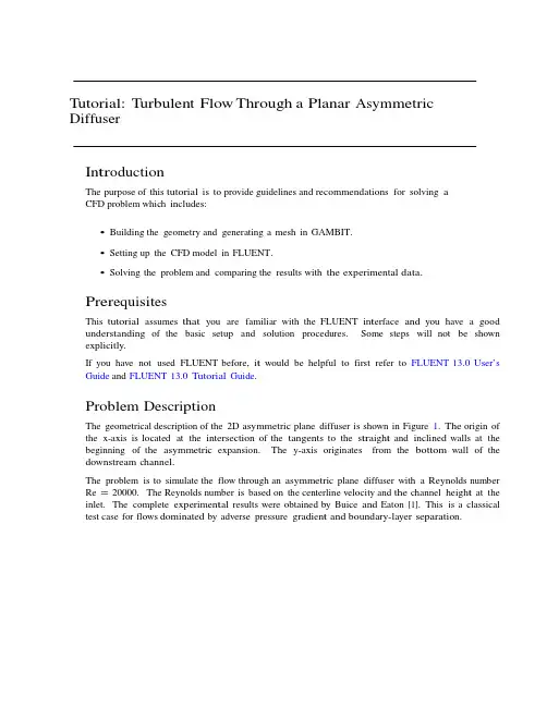
T utorial: T urbulent Flow Through a Planar A s ym metricDiffuserIn t r o ductio nThe purpose of this tutorial is to provide guidelines and recommendations for solving aCFD problem which in c lu des:• Building the geometry and generating a mesh in GAMBIT.• Setting up the CFD model in FLUENT.• Solving the problem and comparing the results with the experimental d ata.Prer equi sit esThis tutorial assumes that you are familiar with the FLUENT in t e rfac e and you have a good understanding of the basic setup and solution procedures. Some steps will not be showne x plicitly.If you have not used FLUENT before, i t would be helpful to first refer to FLUENT 13.0 Us er’s Guide and FLUENT 13.0 Tutorial Guide.Problem Descr i pti onThe geometrical description of the 2D asymmetric plane diffuser is shown in Figure 1. The origin of the x-axis is located at the intersection of the tangents to the s tr aigh t and inclin e d walls at the beginning of the asymmetric expansion. The y-axis originates from the b ottom wall of the downstream c h annel.The problem is to simulate the flow through an asymmetric plane diffuser with a Reyn olds number Re = 20000. The Reynolds number is based on the centerline velocity and the channel heigh t at the inlet. The complete e xp erime n t al results were obtained by Buice and Eaton [1]. This is a classical test case for flows dominated by adverse pressure gradi e n t and boundary-layer s eparati on.Figure 1: Aysmmetric Planar Diffuser GeometryPrepar at io n1. Copy the mesh file, asymmetric.msh and the profile file, channelu.prof to y our workingd irectory.Fluen t Case Setup and Sol uti onStep 1: Mesh1. Start FLUENT 2DDP.2. Read the mesh file, asymmetric.msh.File −→Read −→ Ca s e...3. Scale the mesh.Mesh −→Scale...(a)Select Specify Scaling Factors, and specify values of 0.1 for both Xand Y(b)Click Scale and close the pan el.4. Check the mesh.Mesh −→CheckFLUENT will perform various checks on the mesh and will report the progress in t he console window. If no error messages are reported in the FLUENT window, the mesh check was successful. Step 2: Mo d e ls1. Keep the default General settings.Define −→General2. Enable the realizable k-epsilon turbulence m o del.Define −→Models −→Viscous...(a) Enable k-epsilon (2 eqn) under Model.(b) Enable Realizable under k-epsilon Model and Enhanced Wall Treatment under Ne a r-Wall T r e atment.Note: You have created a very fine near wall mesh in GAMBIT in anticipation of the use of Enhanced Wall Treatment with the turbulence models. A f t e rc a l c u l a t i n g t h e s o l u t i o n,t he xy plot tool in FLUENT can be used toverify the adequacy of the near wall mesh.(c) Click OK to close the pan el.Step 3: Materials and Operating C ondi tionsThe fluid is standard air with constant density so there is no need to visit the materials and operating c on dit ions pan el.Step 4: Boundary C ondit ionsIn order to obtain a fully-developed channel flow at the inlet, you can either extend the channel sufficiently long in the upstream direction, or separately compute a fully-developed channel flow using the same turbulence model for this problem (i.e., the same R ey n ol ds number). Take the latter approach in this tutorial to minimize the size and CPU tim erequired by the model. Profiles of u, v, k, and ε are stored in the file called channelu.prof.This fully-developed channel flow uses the inlet velocity (at the centerline) calculated as follows (the given Reynolds number Re = 20000 is based on the channel height and c enter- line velo ci t y):1. Read in the profi les.Define −→Profiles...(a) Click Read... and select the file channelu.prof.(b) Close the panel.2. Set the boundary conditions for velocity inlet (inlet v).(a) Selec t Components as the Velocity Specification Me th o d.(b) Selec t inner x-velocity for X-Velocity (m/s) and inner y-velocity for Y-Velocity (m/s). (c)Selec t K and Epsilon as Turbulence Specification Me th o d.(d) Selec t inner turb-kinetic-energy for Turb. Kinetic Energy and inner specific-diss-ratefor Turb. Dissipa t i on Rate.The name ’inner’ refers to the to the zone where the profiles were exported f r om.3. Use the d e f aul t No-slip boundary conditions for both the w al ls.4. Set the boundary conditions for pressure ou tle t(outlet).(a) Selec t In t ensit y and Viscosity Ratio for Turbulence Specification Me th o d.(b) Specify a value of 10 for both Backflow Turbulence Intensity and Backflow T urbu-lence Viscosity R atio.Step 5: Soluti on1. Set the solution methodsSolve −→Methods...(a) Select SIMPLEC for the pressure-velocity coupling scheme(b) Click OK to close the panel2. Set the solution controlsSolve ControlsChange the Momentum under-relaxation factor from 0.7 to 0.3. Otherwise keep the default values for the other entries.2. Initialize the s ol ution.Solve −→Initialization…(a) Selec t all-zones in the Compute From drop-down list. (b)Click Initialize3. Use default convergence criteria for all r e sid uals.4. Set up a monitor for wall-shear stress on the w all.Solve −→Monitors… then click Create… below Surface Monitors(a) Enable Plot and Print(b) Enable Plot and Pri nt.(c) Select Area-Weighted Average in the Report Type drop-down list(d) Selec t Wall Fluxes... and Wall Shear Stress in the Report Of drop-down lists.(e) Selec t wall bottom and wall top under Su rf ac es.(f) Click OK to close the pan el.Step 6: Define Custom Field F uncti onsDefine −→Custom Field F unctions...1. Selec t Mesh... and X-Coordinate in the Field Functions drop-down list, and click Selec t.2. Click the buttons /, ., and 1 in a sequence in the Custom Field Function Ca lc u lato r Pad3. Specify x-by-h as the New Function Name and click Define.4. Close the p anel.Step 7: Iterations and C onvergence1. Start the calculations by requesting 1000 iterati ons.Solve −→Run Calculation...Click the Calculate button. Due to the default convergence criteria based on the reduction of the level of the r esi d uals, the solution will converge after just over 300 iterations. Though the calculations have proceeded smoothly so far, two things need to be not ed:(1) The monitor plot shows that the average surface shear stress (on the walls) has not yetreached a constant valu e.(2) You have used the first-order upwind scheme for the convective terms of the governingequations. This scheme is numerically diffusive. Hence it should not be u se d forobtaining the final r esu lts.Switch the discretization scheme for convective terms for the momentum and turbulence equations to second-order u p wind.2. Save the case and data files (asdn3L-initial.cas.gz).3. Change the reference v al ues.Report −→Reference Values...in(a) Change the Velocity value to 2.921469.(b) Change the Length value to 0.1.(c) Click OK to close the pan el .4. Plot the initial r e sults.Display --> Plots… --> XY Plot(a) Des elec t Node Values and Position on X Axis under Option s .(b) Selec t Wall Fluxes... and Skin Friction Coefficient under Y Axis Fun c tion . (c) Selec t Custom Field Functions... and x-by-h under X Axis Fun c tion .(d) Click Load File... and select the cf top.xy file and click OK. Experimental data for skin friction coefficient (C f = τw /0.5ρU 2 ) for the top wall and bottom wall are stored in cf top.xy and cf bot.xy r es pe cti vely .(e) Change the line and symbol style for Curve 0.i. Click on Curves... in the Solution XY Plot pan el.ii. Make the changes as shown in the p anel. iii.Click Apply and close the pan e l.(f)Selec t wall top under Surfaces and click Plot.(g) Repeat the same procedure for bottom wall by loading file cf bot and sele ctin g wall bottom under Su rf ace s.Figure 3: Skin Friction Coefficient Vs x/h (rke - Unconverged Solution) for Top W allFigure 4: Skin Friction Coefficient Vs x/h (rke - Unconverged Solution) for Bottom W a ll5. Change the Discretization scheme to Second Order Upwind for all e qu ation s.6. Disable convergence check for all residu als.Solve −→Monitors −→Res i dual...7. Increase the number of iterations to 4000 and continue the calculation until the monitored quantityb e come s ac on s tan t v alu e.You can see the residuals of all the equations also have dropped below 5 orders of magnitude, so t h e solution can be taken as c onver ge d.8. Save the case and data files (asdn3L-rke.gz).9. Change the viscous model to SST k-omega.Define −→Models −→Viscous...10. Set the boundary conditions for inlet_v(a) Set the Spec. Dissipation Rate to inner specific-diss-rate.11. Continue the calculation with more iterations until the monitored quantity b e come s a c on s tan tv alu e.12. Save the case and data files (asdn3L-sst.gz).Step 8: P ostpr oces singResults and DiscussionDefine a new custom field function as shown below. This will make comparison of the skin friction on the lower wall more convenient.Plot C f for the top and the bottom walls versus data as explained in this tutor ial, (Figures 5 and 6). Compare the results with those obtained from the unconverged soluti on. There is a very sub s tan t ial differe n c e.The predictions for C f along the top wall are substantially different (lower) than the exp er imental data by the realizable k-εmodel. The main reason for the failure is due the fact that it does not correctly predict the size of the sep ar at i on/r e cir culation zone along the incl ine d wall.On the other hand, SST k-ωis the only turbulence model among all the two-equation turbu- lence models which can successfully capture the recirculation zone. SST k-ωmodel’s pr e dic- tion of C f on the top wall is good (see Figure 7), but along the bottom wall it predicts the flow separates slightly upstream of the actual separation point (see Figure 8).Figure 5: Skin Friction Coefficient Vs x/h (rke - Converged Solution) for Top Wal lFigure 6: Skin Friction Coefficient Vs x/h (rke - Converged Solution) for Bottom W allFigure 7: Skin Friction Coefficient Vs x/h (sstkw) for Top Wal lFigure 8: Skin Friction Coefficient Vs x/h (sstkw) for Bottom W allGrid Independence StudyTest whether the converged results (from the SST k-ωmodel: asdn3L-sst.cas.gz, asdn3L-sst.dat.gz) obtained so far are independent of the grid resolution, you can either uniformly double the total cell count, or use the grid adaption feature of the solver to achieve the objective mor e effici en tly.Grid independence is attained when further mesh refinement yields only small andinsignif icant changes in the solution fields. You can use many possible criteria toadapt the mesh. Here we choose the pressure gradient. The separation/recirculationzone should be sensi tive to the computed pressure gradient of the flow. If you proceedfrom your own c a l cul at i on, first save the case and data before attempting any adaptionsince any change is ir r evers ible.1. Open the Gradient Adaption pan el.Adapt −→Gr adi e nt...(a) Ensure Pressure... and Static Pressure is selected in the Gradients Of dr op-down list.(b) Click Compute.This will list the current Max and Min gradients in the boxes.You can use the so-called “10-percent rule” to determine the adaption thr eshol d:to refine the mesh wherever the gradient exceeds 10% of the maximum level.(c) Enter a value of 8.7e-07 for the Refine Threshold and click Ma r k. (d) Click Manage...button to open t h e Manage Adaption Registers pan el.i. Plot the adaptively refined mesh by clicking Display.In general, it is desirable to have the marked cells clustered in a c ontiguous manner.(If they are not, delete the register and reduce the R efinement Threshold and do it again.) For the the current problem we have incr e ase d about 10000 cells (about 17% more) and they are mainly concentrated around the inclined section of the channel. We consider it to be satisfactory and pr ocee d.ii. Click Adapt and click Yes when prompted Hanging-node mode: Ok to a dap t grid?.(e) Continue the iterations until the case is converged.(f) Save the case and data files (asdn3L-sst-adapt.gz).(g) Plot the results, (Figures 9 and 10).It can be seen that there are no detectable changes from the previously obtaine d results (except some small improvement over the range of 10 < x/h < 20), s o now you can say that the converged solution for this case is grid-indep endent.Figure 9: Skin Friction Coefficient Vs x/h (sstkw) After Grid Adaption for Top W allFigure 10: Skin Friction Coefficient Vs x/h (sstkw) After Grid Adaption for Bottom W allSumm aryIn this tutorial, you performed a simulation of steady-state turbulent flow through an asymmetric, planar diffuser by using the popular realizable k-ε model. The calculated skin friction coefficients (C f) at the top and bottom of the diffuse r walls were compared with e xp e r ime n t al data reported by Buice and Eaton. Be t we en the t w o-equati on turbulence models, only the SST k-ωmodel gives reasonable predictions of the skin fr ic t ion and the recirculation z on e.You have also le arn ed how to use FLUENT´s grid adaption feature to test whether or not th e calculation is grid independent, without having to uniformly double up the cell coun t in the whole flow d om ai n.Refe rence s[1] C.U. Bruice and J.K. Eaton. Experimental investigation of flow through an asymm et ric plane diffuser. Technical Report No. TSD-107, Thermosciences Division, Dept. of MechanicalEngineering, Stanford University, Stanford, CA, USA, Augu s t 1997.。

沙尘环境下交通流跟驰模型及仿真谭金华【摘要】Driver's sight would be affected by sand-dustenvironment,resulting in additional reaction time to identify road and traffic conditions,which may cause safety problems.To explore the impact of sand-dust environment on traffic flow,this study proposes an extended car-following model based on driving behaviors under sand-dust environment(SDM).Through linear stability analysis and numerical simulation,the results show that the unstable region of SDM enlarges with increasing the va lue of the parameter α,which indicates that it can weaken the stabilization of traffic system.Besides,the more severely the traffic flow is affected by sand-dust environment,the greater the dispersion of vehicle speed will be,and the wider the fluctuation range of acceleration will be.Therefore,the sand-dust environment will lead to traffic flow involved in unsafe state,which increases traffic accident probability.%沙尘环境下,沙、尘土及其他异物会影响驾驶员的视线,让驾驶员额外增加辨别道路条件和周围交通状况的反应时间,带来一定的交通安全隐患.为探讨沙尘环境对道路交通流的影响,本文建立了基于沙尘环境下驾驶行为的跟驰模型(SDM).线性稳定性分析和数值模拟结果表明:沙尘环境下,SDM的稳定区域缩小,交通流出现小的扰动后,难以恢复到稳定状态;而且,交通流受沙尘影响越严重,车辆速度的离散性越大,加速度的波动幅度也越大.可见,沙尘环境使交通流处于不安全的状态,易引发道路交通事故.【期刊名称】《交通运输系统工程与信息》【年(卷),期】2018(018)003【总页数】5页(P63-67)【关键词】交通工程;沙尘环境;跟驰模型;数值模拟;交通安全【作者】谭金华【作者单位】中南财经政法大学信息与安全工程学院,武汉430073【正文语种】中文【中图分类】U491.30 引言沙尘、冰雪、降雨和浓雾等不利天气会影响道路交通的正常运行，甚至引发事故.据统计[1]，2005—2014年间全国不利天气条件下，平均每起事故死亡人数位居第2的是沙尘天气，达到0.455人/起.为了探讨不利天气条件对道路交通的影响，许多学者从微观的角度，建立交通流模型.Shi J.等[2]考虑浓雾下的驾驶行为，建立单车道元胞自动机模型，研究雾天对交通效率、事故和汽车有害气体排放等的影响.谭金华等[3]建立了高速公路双车道间断放行模型，研究浓雾天气时，不同管理措施下发生交通事故的概率.张卫华等[4]考虑降雨情形下，驾驶员换道行为的变化，建立高速公路元胞自动机模型.赵韩涛等[5]研究了冰雪天气条件下，城市道路中的单、双车道微观交通流模型，探讨冰雪天气对交通流的影响.然而，沙尘天气对道路交通流的影响，尚未得到广泛关注.鉴于此，本文首先分析沙尘环境对驾驶员操作造成的不利影响，建立基于沙尘环境下驾驶行为的交通流跟驰模型.然后，通过线性分析，探讨沙尘环境下交通流的稳定性.最后，通过数值模拟，研究本文所提出的模型中，沙尘环境对车辆速度、加速度和车头间距等交通流参数的影响.1 跟驰模型的建立Newell模型[6]认为，若假定第n辆车在第t时刻所在的位置为xn(t)，则第n辆车的速度dxn(t)dt，是由与其前面第1辆车(即第n+1辆车)的车头间距Δxn(t)决定的，且Δxn(t)=xn+1(t)-xn(t).延迟时间T之后，在Δxn(t)的间距内，车辆达到最优速度V(Δxn(t))，即式中：T由人的正常反应延迟和车辆响应时间延迟组成.沙尘环境下，沙、尘土及其他异物会影响驾驶员的视线，让驾驶员额外增加辨别道路条件和周围交通状况的反应时间，即总的反应时间会大于T，Newell模型应调整为式中：αT表示额外增加的反应时间，α为可变参数.考虑到沙尘环境下车辆行驶速度会降低，本文用ε表示行驶速度降低的程度，0＜ε＜1.综上所述，沙尘环境下(Sand-Dust Environment,SD)的跟驰模型，可以表达为式(3).为叙述方便，后文简称此模型为SDM.为将SDM化简，对式(3)左边的在t处做泰勒展开，保留至第2项,可得联合式(3)和式(4)，可得经整理，得到SDM简化后的表达式为对于式(6)的最优速度V(Δxn(t))，本文选取Helbing和Tilch[7]提出的OV函数，即式中：lc表示车长，且lc=5，C1=0.13,C2=1.57,V1=6.75,V2=7.91.2 线性稳定性分析为研究沙尘环境对道路交通流的影响，本文对SDM进行线性稳定性分析.交通流的初始状态为所有车辆的车头间距恒定为b，且以匀速V(b)行驶，第n辆车在第t 时刻的位置为设yn(t)为第t时刻交通流中出现的1个小的扰动，则进一步可推出第n+1辆车的位置为第n辆车与第n+1辆车的车头间距Δxn(t)，经计算得到联合式(6)～式(11)可得经推导计算，可得式(13)，满足此条件时交通流处于稳定状态[8].求解式(13)，得到由文献[6]和[7]可知，1 T即为交通流的敏感系数，该值越大，则表明交通流越稳定.当该值大于2εV′(b)(1+α)时，小的扰动下，交通流可经过一段时间后恢复稳定；若该值小于2εV′(b)(1+α)，则出现小的扰动后，无论经过多长时间，车辆的速度和车头间距都不可能再稳定下来.因此，SDM的中性稳定条件为图1为车头间距与敏感系数的临界曲线，α的取值分别为0.0，0.2和0.4，ε=0.8.临界曲线下方为不稳定区域，当α和T的取值在此区域时，交通流出现1个小的扰动后，将不再回到稳定状态.由图1可见，α越大，不稳定区域越大，说明沙尘环境对交通流的稳定性有负面影响.图1 不同α下的临界曲线Fig.1 The neutral stability lines for differentα3 数值模拟为探讨沙尘环境对车辆速度、加速度和车头间距等交通流参数的影响，本文应用Matlab R2014b编程进行数值模拟.在周期边界条件下，道路长度为L，车辆数量为N.交通流的初始状态为车辆均匀地分布在道路上，即xn(0)=n⋅L/N，本文根据文献[8]和[9]，取L=1 500，N=100，ε=0.8，初始扰动x1(0)=10，延迟时间T 分别设为0.5和1.2.模拟时，每隔0.1 s采集1次数据.图2为α=0.2，T=1.2时所有车辆的车头间距.图2(a)表示t=50s时车头间距的失稳状况，图2(b)表示经过足够长的时间t=8 000s后车头间距的变化.图2(a)和图2(b)均显示车头间距处于不稳定状态，说明在给定的条件下，交通流出现的扰动不能被吸收.由SDM的稳定性分析结果可知，α=0.2，T=1.2时，交通流处于不稳定区域.图3则为α=0.2，T=0.5条件下，交通流在时间t=50s和t=8 000s时所有车辆的车头间距变化情况.图3(a)显示t=50s时，车头间距出现波动，但和图2(a)相比较而言，波动幅度较小.图3(b)显示，交通流经过8 000 s的演化，车头间距波动幅度为0，重新回到稳定状态.从图3可知，α=0.2，T=0.5时，交通流处于稳定区域.图2 T=1.2时车头间距Fig.2 The headway underT=1.2图3 T=0.5时车头间距Fig.3 The headway underT=0.5因此，图2和图3的数值模拟结果和稳定性分析结果是一致的.而且，随着T的增大，即敏感系数降低，车头间距的波动幅度也增大.车辆速度与交通安全有直接的关系.交通系统中，车辆速度的离散性越大，事故率往往越高，事故损失也越大.图4为T=0.5，α取不同数值时，速度波动随着时间增大向后传播的演化图.当α=0.0和α=0.2时，随着时间的增大，车速的波动幅度越来越小，即车辆速度的离散性越来越小；当α=0.4时，车辆速度的离散性随着时间增大没有明显的变化.比较图4(a)～(c)可知，α的取值在区间[0.0,0.4]时，其与车速离散性是正相关的.所以，沙尘环境会影响车辆速度的离散性，且交通流受沙尘环境的影响越严重，速度的离散程度越大.图4 速度的演化Fig.4 Space-time evolution of the velocity under differentα加速度能够反映交通流中可能存在的急加速、急刹车现象.图5表示T=0.5，在不同α条件下，交通流在t=50s时，所有车辆的加速度变化.图5中，α分别为0.0，0.2和0.4.其中，α=0.4表示交通流受沙尘影响相对最严重的情形，从图5(c)可知，此时加速度的波动幅度最大.图5 t=50s时车辆加速度Fig.5 The acceleration under differentαwhent=50s交通流在经过时间t=8 000s后，α=0.0和α=0.2时所有车辆的加速度均为0.当α=0.4时车辆的加速度如图6所示.可见，α=0.0和α=0.2时，即α和T的取值处于稳定区域，从t=50s至t=8 000s的过程中，车辆的速度逐渐趋于稳定.而当α=0.4时，加速度的波动幅度增大，交通流中可能会出现一些急加速和急减速现象，影响交通安全.图6 t=8 000s时车辆加速度(α=0.4)Fig.6 The accelerationunderα=0.4whent=8 000s4 结论沙尘天气是影响道路交通安全的重要环境因素.本文基于沙尘环境下的驾驶行为建立交通流跟驰模型.由扰动起源事故理论[10]可知，交通系统中出现的扰动(Perturbation)是引发事故的风险因素.根据此理论，当交通流出现扰动后，本文对SDM进行线性稳定性分析，结果表明沙尘环境下稳定区域缩小.研究发现，数值模拟结果与稳定性分析结果一致，即沙尘环境不利于受扰动的交通流恢复至稳定状态，而且交通流受沙尘影响越严重，车辆速度的离散程度越大，加速度的波动幅度也越大.在沙尘环境下，交通流出现的扰动不仅难以被吸收，还可能呈现不断传播态势，使车头间距、速度的离散性和车辆加速度都处于不安全状态，极易发生交通事故.因此，应加强沙尘环境下交通安全管理，采取一定应对措施，控制发生事故的风险.【相关文献】[1]宁贵财,康彩燕,陈东辉,等.2005—2014年我国不利天气条件下交通事故特征分析[J].干旱气象,2016,34(5)：753-762.[NING G C,KANG C Y,CHEN D H,et al.Analysis of characteristics of traffic accidents under adverse weather conditions in China during 2005-2014[J].Journalof Arid Meteorology,2016,34(5)：753-762.][2]SHI J,TAN J H.Traffic accident and emission reduction through intermittent release measures for heavy fog weather[J].Modern Physics Letters B,2015,29(25)：1550148.[3]谭金华,石京.浓雾下高速公路双车道间断放行措施[J].清华大学学报(自然科学版),2016,56(9)：985-990.[TAN J H,SHI J.Two-lane freeway intermittent release measures in heavyfog[J].Journal of Tsinghua University(Science and Technology),2016,56(9)：985-990.][4]张卫华,颜冉,冯忠祥,等.雨天高速公路车辆换道模型研究[J].物理学报,2016,65(6)：184-192.[ZHANG W H,YAN R,FENG Z X,et al.Study of highway lanechanging model under rain weather[J].Acta Physica Sinica,2016,65(6)：184-192.][5]赵韩涛,聂涔,李静茹.冰雪条件下的交通流元胞自动机模型[J].交通运输系统工程与信息,2015,15(1)：87-92.[ZHAO H T,NIE C,LI J R.Cellular automaton model for traffic flow underice and snowfall conditions[J].Journal of Transportation Systems Engineering and Information Technology,2015,15(1)：87-92.][6]NEWELL G F.Nonlinear effects in the dynamics of car following[J].Operations Research,1961,9(2)：209-229.[7]HELBING D,TILCH B.Generalized force model of traffic dynamics[J].Physical Review E，1998,58(1)：133-138.[8]JIN S,WANG D H,XU C,et al.Staggered car-following induced by lateral separation effects in traffic flow[J].Physics Letters A,2012,376(3)：153-157.[9]艾力·斯木吐拉,李鑫,马晓松.驾驶员反应特性在沙漠环境中的表现[J].安全与环境学报,2008,8(4)：143-147.[ISMUTULLA E,LI X,MA X S.On-spot testing of the reaction characteristics of drivers in the desert conditions[J].Journal of Safety and Environment,2008,8(4)：143-147.] [10]田水承,景国勋.安全管理学(第2版)[M].北京：机械工业出版社,2016.[TIAN S C,JING GX.Safety management(Second Edition)[M].Beijing：China Machine Press,2016.]。

2009年7月水 利 学 报SHUILI XUEBAO第40卷 第7期收稿日期:2008-11-06基金项目:国土资源大调查项目(1212010634611);基本科研业务费项目(SK07013)作者简介:王昭(1969-),女,汉族,副研究员,博士,主要从事环境水文地质方面的研究。

E -mail:bike2002d@文章编号:0559-9350(2009)07-0830-08华北平原地下水中有机物淋溶迁移性及其污染风险评价王 昭,石建省,张兆吉,费宇红(中国地质科学院水文地质环境地质研究所,河北石家庄 050061)摘要:根据有机污染物的物理化学性质,估算了91种有机物在土壤中的半衰期和有机碳吸附系数,并分析了这些有机物在土壤中的淋溶迁移性。

结果表明:对于所研究的污染物,它们的地下水污染指数与其有机碳吸附系数有着很好的负相关性,这为评价地下水中主要有机污染物的污染指数(淋溶迁移性)提供了简易方法。

所评价的91种有机物中,38种具有高淋溶和迁移性,易对含水层造成较大范围的污染。

通过分析发现,华北平原区域地下水中主要有机物的检出率与其淋溶迁移性有着一定的相关性。

因此,地下水污染指数法的应用将有助于预测有机物对地下水的污染风险。

关键词:华北平原;地下水有机污染;EPI Suite;地下水污染指数(GUS)中图分类号:X143文献标识码:A1 研究背景自20世纪70年代后期开始,地下水有机污染已引起人们的高度重视。

如美国的50个州均有微量有机物的报道[1]。

1987年美国地下水中已发现了175种有机化合物[2]。

1990年,中国环境监测总站周文敏等[3]提出了反映我国环境特征的中国环境优先控制污染物 黑名单 ,共有14类68种优先控制污染物,其中有毒有机化合物12类58种。

但在我国,地下水的有机污染调查与研究尚处于初级阶段,为了更加科学地分析地下水有机污染调查的数据,对地下水污染风险进行正确的评价,可以先根据有机物本身性质来预测它们对地下水的污染威胁以及其在水土中的迁移性等。

首都师范大学学报(自然科学版)第25卷　专辑2004年12月Journal of Capital N ormal University(Natural Science Edition )V ol.25Dec.　2004SCS 模型在密云石匣试验小区降雨径流量估算中的应用张美华　王晓燕　秦福来(首都师范大学资源环境与旅游学院,北京　100037)摘要 利用密云县石匣小流域2001年的6场降雨及径流观测数据,应用SCS 模型计算参数I a 在不同水平下22个试验小区的径流量,依据实测值对计算值进行了调整,得出了适合该小区的参数C N 的范围,并将参数进行检验,得到了较好的结果.关键词:SCS 模型,C N 值,降雨量,径流量.中图分类号:P 332收稿日期:2004211209 SCS 模型是美国农业部水土保持局研制的小流域设计洪水模型,计算过程简单,所需参数较少,资料易于获取,对观测数据的要求不很严格,尤其适用于资料缺乏地区,并且有效地考虑了流域下垫面的特点,是一种较好的计算小流域降雨径流量的方法.目前在美国和其它一些国家得到了广泛的应用,SCS 模型在我国的应用开始于二十世纪80年代,许多专家和学者将此模型应用于小流域工程规划、流域水土保持、城市径流、无资料流域的径流模拟等研究中[1].但由于我国和美国的地区之间在气候、土壤、种植方式等多方面,存在广泛差异性,直接应用美国测定的C N 值,不太适合国内的情况,所以各地在应用时都作了因地适宜的修正.对密云石匣小流域的研究中,符素华通过几种模型的比较,得到的结论是虽然SCS 模型的确定性系数没有G AM L 和Phillip 计算结果的模型确定性系数较高,但若无降雨过程资料可用SCS 径流曲线数进行径流计算[2].本研究就是在此基础上,利用北京密云石匣22个试验小区2001年的6场降雨资料,用SCS 法计算在不同的参数水平下的降雨径流量,将计算值与实测值相比较,尝试探讨适合石匣小区的合理参数,对农田非点源污染物输出的模拟以及水土资源的合理利用都有重要的意义[3].1　SCS 模型简介111　基本原理Boughton 、M ockus[4,5]对此模型的产生、演变、以及模型方程的修正优化做出了巨大贡献.最初的径流方程没有考虑降雨初损,后经过修正.SCS 径流模型能反映不同土壤类型、不同土地利用方式及前期土壤含水量对降雨径流的影响,它是基于流域的实际入渗量与实际径流量之比等于流域该场降雨前的最大可能入渗量(或潜在入渗量S )与最大可能径流量之比的假定基础上建立的,初损I a 受土地利用、耕作方式、灌溉条件、枝叶截留、下渗、填洼等因素的影响,它与土壤最大可能入渗量S 呈一定的正比关系,美国农业部土壤保持局在分析了大量长期的实验结果基础上,提出了二者最合适的比例系数012,即I a =012S 最后修正的公式即[6]:Q =(p -012S )p +018S　p ≥012SQ =0p <012S112　参数CN确定为了估计流域土壤的最大可能入渗量S,SCS模型提出了一个径流曲线数(runoff curve number,记为C N)指标作为反映降雨前流域特征的一个综合参数,则有:S=(25400ΠCN)-254 由此式可见:C N值越大,S值越小,越易产生径流.决定C N的主要因素为土壤前期湿度、土壤类型、植被覆盖类型、管理状况和水文条件,同时坡度也对C N有一定影响.C N的确定分为三个步骤:①根据土壤水分的最小渗透率划分而成的四组水文土壤类型(见表1)来确定研究流域土壤的水文土壤组属性.表1　SCS水文土壤组定义指标[7]土壤类型最小下渗率(mmΠh)土壤质地A>7126砂土、壤质砂土、砂质壤土B3181～7126壤土、粉砂壤土C1127～3181砂黏壤土D0100～1127　黏壤土、粉砂黏壤土、砂粘土、粉砂黏土、黏土 ②考虑所研究流域土壤前期湿度条件,并参照AMC三级划分指标来客观定义土壤前期湿度.AMCⅠ:土壤干旱,但未到达植物萎蔫点,有良好的耕作及耕种.AMCⅡ:发生洪泛时的平均情况,即许多流域洪水出现前夕的土壤水分平均状况.AMCⅢ:暴雨前的5天内有大雨或小雨和低温出现,土壤水分几乎呈饱和状况.③综合研究流域土地利用方式、水文土壤组特征和前期湿度条件,在由美国农业部土壤保持局提出的C N表中查找并确定适用所研究流域的C N值.若AMCⅡ的C N已知,条件AMCⅠ和AMCⅢ相应的曲线数可以根据一下的公式计算而得.CN(Ⅰ)=412CN(Ⅱ)Π[10-01058CN(Ⅱ)]CN(Ⅲ)=23CN(Ⅱ)Π[10-0113CN(Ⅱ)]表2　前期土壤湿润程度等级划分[7]AMC前5d降雨量(mm)生长期休止期Ⅰ<13>28Ⅱ13～2836～53Ⅲ>28>532　SCS模型的应用211　石匣小流域及试验小区自然概况密云石匣小流域地处北京市密云水库的东北,按水系划分属潮河下游,为土石浅山丘陵区.土壤类型为洪积冲积物母质上发育的褐土,质地为轻壤土,土层较深厚.流域多年平均降水量为66118mm,80%集中在6～9月[8].小区按坡度划分为:3°～8°(小区17、18、19、20)、8°～15°(小区4、5、6、7)、15°～25°(小区1、2、3、11、12、13、14、15、16)、大于25(小区8、9、10)四个等级.按土地利用分为耕地(1号陡坡开荒、6、18、20号坡耕地玉米、17号梯田玉米)、林地(2号水平条果树、7号水平条山楂、10号鱼鳞坑刺槐、12号鱼鳞坑侧柏)、荒坡地(5、9号)、自然坡(11、13、14、16、19号,且11、13、14小区坡度越来越长)、休闲地(3、4号)、8号为封育地以及15号为牧草地、21和22为标准小区.212　SCS公式的修正21211　前期损失量的修正在降雨径流损失过程中,地面不平整产生的填洼、下渗、壤中流和地下径流是主要的损失量.美国的降水年内分布比较均匀,密云地区的降水主要集中在夏季的6～9月,尤其是7、8月份,多有大暴雨,下渗雨量少,约为40%,所以在应用模型的过程中, I a取值范围扩大为0115～0125S’,分别取0115、012、0125进行修正.21212　C N值的修正由于所研究范围很小,根据密云水库地区的土壤资料,石匣小区的土壤水文组可以近似为B组类型,另由石匣试验小区的设计资料获得每个小区的土地利用方式及覆被情况,根据模型提供的C N表按照各个小区的前5天是否有降水、降雨量、雨强、土地利用措施,最后确定土壤前期湿润程度为AMC Ⅰ.根据SCS表查得AMCⅡ时的C N值,选取其中5场降雨随着Ia的变化进行C N的修正;参照实际径流量在Excel中人工调整C N值直到计算径流量和实际径流量相符合为止.所调整的C N值图如下所示:除了1、3小区数值波动较大,其他小区数值在60左右波动.若降雨量、雨强都很大,则在计算径流量时根据雨情人为将C N值在60的基础上相应提高,反之亦然.21213　修正后的模型有效性的验证如表3,两者虽有一定的误差,误差最大为651首都师范大学学报(自然科学版)2004年图1　调整后的CN值0157812,最小为01002141,但结果是有效的.3　SCS讨论311　降雨因素的影响当雨量大、雨强大、降雨历时短时,小区容易出流.这时初损也很大,初损参数一般为0125时,计算径流量和实际径流量相接近.例如:2001年6月28日的一场降雨,降雨量为4515mm,最大雨强为3615 mmΠh,22个小区只有12号小区没有出流,此时确定C N值时应该偏大一些,因为用SCS模型计算出来的径流量会比实际值偏小[2];当雨量大、雨强小、历时长时,初损参数定为012～0125,此时计算的径流量会很大,但实际径流量并不大,此时的C N值应该取值小一些.例如:2001年7月21日,雨量为47,历时13时10分,雨强为3157mmΠh,只有6个小区出流,且出流量小.以1小区为例,6月28日的径流量为3185,7月21日的径流量为0111.表3　试验小区径流量验证表小区号降雨时间实测值计算值误差18Π24Π20010127012317610114162638Π24Π2001012501303136-012125448Π24Π20010124012317610103432968Π24Π200101170116963601002141158Π24Π2001010740107359701005446188Π24Π200101301473437-0157812208Π24Π200101250123176101072956218Π24Π2001016901798055-01156628Π24Π2001016601680537-0103112312　土地利用类型的影响在小区的几种利用方式中,耕地、休闲地易出 流,林地不易出流,尤其是鱼鳞坑林地,自然坡和荒坡地居中.耕地的C N值较稳定,例如18小区,在几次降雨中,C N值为60195、61109、60110、60181、62110,最大为6211,最小值为6011;初损参数在0115～012时计算值与实测值最接近.自然坡的保水效果也很好,C N值在56～58之间,初损参数为012.与自然坡相比,坡荒地的C N值变动较大,变化范围为59～64之间.可见,在相同的降雨条件下,前期土壤湿润程度状况越干,不同的土地利用类型之间对径流量的产生影响也越大[9].313　坡度、坡长的影响9号小区与5号小区相比,两者土地利用方式相同,但9号小区的坡度大,同一场降雨,2001年6月15号,9号小区的径流量为0142m3,5号小区为0108m3.当降雨量大时,坡度越长,径流量也越大,6月28日的降雨,11号小区坡长是5m,径流量是0124,14号小区坡长15m,径流量是0128.此外,小区植物覆盖度会随着植物的生长而向增大的方向发展,对降雨截流亦有一定的影响.314　结　论SCS模型所需资料简单易取,它不仅能反映不同土壤和地表覆被条件的产流情况,而且充分考虑了土壤前期湿度对降雨产流的影响.通过对初损Ia 和参数C N的合理调整,在缺乏降雨资料的小流域径流量计算中不失为一种较为适用的方法模型.但没有考虑降雨历时和雨强对初损及C N值的影响,会不可避免地影响模型的估算精度及使用效果;另外SCS所提出的前期土壤湿度等级划分及土地利用与管理方式是基于美国的分类,在我国应用时不同的地区不同的使用主体的主观性太强,依赖于使用者的经验技术和知识水平.本文通过对初损参数和C N的修正,得到了可信度较高的结果.但不同的地区在应用时,不能盲目的搬用模型所提供的C N值表.751专辑张美华等:SCS模型在密云石匣试验小区降雨径流量估算中的应用851首都师范大学学报(自然科学版)2004年参考文献1　晋华.SCS模型在岚河流域的应用研究.太原理工大学学报,2003,34(6):735～7362　符素华,刘宝元,等.北京地区坡面径流计算模型的比较研究.地理科学,2002,22(5):604～6083　贺宝根,周乃晟.农田非点源污染研究中的降雨径流关系-SCS法的修正.环境科学研究,14(3):49～514　Boughton W C.A review of the US DA SCS curve number method[J].Australian:Journal of S oil Research,1989,27:511～523 5　M ockus V.Estimation of total(and peak rates of)surface runoff for individual storms.In:Interim Survey Report G rand(Neosho) River Watershed.Exhibit A of Appendix B.U.S.Dep.Agri C(U.S.G ov.print.O ffice:Washington,D.C),1949 6　罗利芳,张科利.径流曲线数法在黄土高原地表径流量计算中的应用.水土保持通报,2002,22(3):58～617　王晓燕.非点源污染及其管理.海洋出版社,2003,43～488　刘振国,符素华.密云石匣小流域水土流失规律研究.北京水利,2000,(3):11～139　史培军,袁艺,陈晋.深圳市土地利用变化对流域径流的影响生态学报,2001,21(7):1041～1049Application of SCS Modal to Estim ate the Q uantity of R ainfall Runoff of Sm all W atershed in Shixia,Miyun CountyZhang Meihua　Wang X iaoyan　Qin Fulai(Res ource,Enviroment&T ourism,Capital N ormal University,Beijing　100037)AbstractUsing the m odel of SCS,runoff of22plots at Shixia watershed,Miyun C ounty,are calculated in different parameter Ia levels.Then the calculated value are adjusted according to the m onitoring data of six storm events,the suitable C N parameter range is als o verified.K ey w ords:SCS m odel,C N,rain fall,funoff.作者简介　张美华,资环学院03级硕士研究生.主要研究方向为生态环境建设与治理。

高速公路交通流模型研究及仿真分析高速公路在现代交通系统中发挥着至关重要的作用。

为了更好地理解和优化高速公路的交通流，研究人员建立了各种交通流模型，其中最著名的有LWR模型、CTM模型和GKT模型等。

本文将探讨这些模型的基本原理和仿真分析结果。

一、LWR模型LWR模型（Lighthill-Whitham-Richards模型）是一种最简单的交通流模型之一。

它基于连续性方程和通量方程，假设道路上的车辆密度和速度是空间和时间的函数。

然后，使用一个自由流速度函数和一个阻尼函数来表示车辆速度和密度之间的关系。

这个模型可以描述交通流的基本特征，如拥堵，瓶颈等。

但由于该模型缺少车辆间互相作用的部分，因此它无法完全捕捉到交通流动态的复杂性。

二、CTM模型CTM模型（Cell Transmission Model）是一种基于单元网格的交通流模型。

该模型将道路划分为许多网格单元，并在每个单元上应用LWR模型。

这种方法可以有效地模拟车辆流量对道路上的拥堵情况的影响。

它还可以处理多个车道和变速公路等复杂的道路拓扑结构。

该模型采用交错网格技术来捕获车辆的交互作用，同时保持模型的简单性。

三、GKT模型GKT模型（Gazis-Koh-Tabak模型）是一种基于宏观观点和马尔可夫过程的交通流模型。

它考虑了车辆之间互相影响的部分，并且通过概率分布模拟车辆的行为。

该模型将道路划分为几个不同的状态，例如自由流状态，饱和状态，拥堵状态等。

车辆会随机地在这些状态之间转移，而这些状态之间的概率转移矩阵可以用实验测量数据来估计。

该模型具有很好的现实逼真性，但是其参数通常比较难以估计。

四、仿真分析为了评估不同模型的预测能力，研究人员通常会使用仿真分析来进行比较。

在仿真过程中，研究人员将建立的模型应用于现实交通流数据，然后对模拟结果进行统计分析和可视化呈现。

通过比较模拟和实际数据之间的差异，研究人员可以评估每种模型的准确性和实用性。

此外，仿真还可以用于评估不同的交通流优化策略的性能，并帮助交通管理人员做出优化决策。

第22卷　第10期2007年10月地球科学进展A DVAN CE S I N E AR T H S C I E N C EV o l.22　N o.10O c t.，2007文章编号：1001-8166（2007）10-1041-07潜流构建湿地氮素转化运移的理论模型研究*宋新山1，邓　伟2，夏永云1（1.东华大学环境科学与工程学院，上海　201620；2.中国科学院成都山地灾害与环境研究所，四川　成都　610041）摘　要：构建湿地中氮素的主要存在形态为有机氮和无机氮，无机态氮主要包括氨态氮和硝态氮两种形态。

一方面，这些氮素之间通过矿化、氨同化、硝化、反硝化、吸附交换、植物吸收等物理、化学及生物学过程相互联系并相互转化；另一方面在构建湿地污水处理系统中，从进水到出水，这些不同形态的氮素又随多孔介质中的饱和流发生运移。

根据氮素的转化机理和溶质运移理论，以构建湿地中氮素的溶质运移模型为基础，将氮素转化的机理过程作为源汇项包括到基本模型中，由不同形态氮素的运移转化模型相联合形成构建湿地中氮素转化运移的理论模型系统。

根据文献调研，给出模型系统参数的参考值，并简要介绍了模型系统的计算机语言求解方法。

该模型为深入研究构建湿地中污水脱氮综合机理提供工具，其结果为以脱氮为目的的构建湿地的设计提供科学参考。

关　键　词：构建湿地；氮转化机理；溶质运移；数学模型中图分类号：X171.4 文献标识码：A1　引　言由于构建湿地表现出的良好脱氮效果、低廉的运行和基建费用、方便的维护管理等特点［1，2］，使得1990年代以后，其不但广泛地应用于生活污水和市政废水处理，而且也有一些工业废水处理的尝试和研究［3，4］。

由于氮素在水环境中的转化行为较复杂，尤其是在构建湿地这样一个复杂的多相环境介质中，脱氮涉及到物理、化学和生物学过程［5，6］，因此构建湿地污水脱氮机理成为研究的热点［2，6～8］。

目前对于氮素转化的单个机理过程已经比较清楚，如硝化、反硝化、矿化等生化过程，传统的污水脱氮过程已有比较成熟的数学模型［9］。