Properties of Bootstrap Moran for Diagnostic Testing a Spatial Autoregressive Model
- 格式:pdf
- 大小:383.39 KB
- 文档页数:28
bootstrapmodelform的用法-回复Bootstrap是一个流行的前端开发框架,提供了丰富的样式和组件,可以大大简化页面的开发和设计过程。
其中一个常用的组件是Bootstrap Model(模态框),它可以用于显示弹出窗口来展示一些内容或执行特定的操作。
而Bootstrap Model Form(模态框表单)是在模态框中添加表单的方式,可以用于用户输入数据和进行提交操作。
下面将介绍Bootstrap Model Form的基本用法以及一些常见的定制化操作。
1. 引入Bootstrap库和jQuery库为了使用Bootstrap Model Form,首先需要在HTML文件中引入相应的库文件。
可以通过CDN方式使用以下链接引入所需的CSS和JavaScript 文件。
<! 引入Bootstrap样式文件><link rel="stylesheet" href="<! 引入jQuery库><script src="<! 引入Bootstrap JavaScript文件><script src="2. 创建一个按钮以触发模态框使用Bootstrap Model Form的第一步是创建一个按钮,点击该按钮时将触发模态框的显示。
按钮可以使用Bootstrap的按钮样式类来实现。
例如,使用以下HTML代码创建一个按钮:<button type="button" class="btn btn-primary"data-bs-toggle="modal" data-bs-target="#myModal">打开模态框</button>其中,`data-bs-toggle="modal"`用于指定按钮点击时触发模态框的显示,`data-bs-target="#myModal"`指定该按钮所触发的模态框的ID。
BootStrapValidator使⽤注意事项(必看篇)如果你使⽤的前端框架是bootstrap,那么前端验证框架就不必考虑了,bootstrapvalidator是最好的选择,它和bootstrap的结合最完美,不过要注意版本的问题,针对bootstrap2和bootstrap3有不同的版本。
下⾯是我遇到的两个注意事项,⾃⼰做个笔记:1、为每个要验证的表单元素添加name属性例如:<div class="form-group"><input type="text" placeholder="请输⼊短信验证码" id="smsCaptcha" name="smsCaptcha" class="form-control"data-bv-notempty data-bv-notempty-message="验证码不能为空"data-bv-regexp="true" data-bv-regexp-regexp="[0-9]{6}" data-bv-regexp-message="验证码格式不正确" ></div> <div class="form-group"><input type="email" class="form-control" id="exampleInputEmail1" placeholder="Enter email"data-bv-notempty data-bv-notempty-message="验证码不能为空" ></div>上⾯这个例⼦中,第⼀个表单元素添加了name属性,第⼆个表单元素没有name属性,⽽这两个表单元素都使⽤了⾮空验证,最终效果如下:从结果可以看出,如果要验证⼀个表单项,则该表单项必须有name属性。
Propertyspring.profiles.activeimportedfromloc。
问题描述最近⽤springboot写后端服务,之前明明可以运⾏的多环境配置,突然不奏效了,报如下错误:org.springframework.boot.context.config.InvalidConfigDataPropertyException: Property 'spring.profiles.active' imported from location 'class path resource [application-test.yml]' is invalid in a profile specific resource [origin: class path resource [ap at mbda$throwOrWarn$1(InvalidConfigDataPropertyException.java:124)at ng.Iterable.forEach(Unknown Source)at java.util.Collections$UnmodifiableCollection.forEach(Unknown Source)at org.springframework.boot.context.config.InvalidConfigDataPropertyException.throwOrWarn(InvalidConfigDataPropertyException.java:121)at org.springframework.boot.context.config.ConfigDataEnvironment.checkForInvalidProperties(ConfigDataEnvironment.java:354)at org.springframework.boot.context.config.ConfigDataEnvironment.applyToEnvironment(ConfigDataEnvironment.java:323)at org.springframework.boot.context.config.ConfigDataEnvironment.processAndApply(ConfigDataEnvironment.java:236)at org.springframework.boot.context.config.ConfigDataEnvironmentPostProcessor.postProcessEnvironment(ConfigDataEnvironmentPostProcessor.java:97)at org.springframework.boot.context.config.ConfigDataEnvironmentPostProcessor.postProcessEnvironment(ConfigDataEnvironmentPostProcessor.java:89)at org.springframework.boot.env.EnvironmentPostProcessorApplicationListener.onApplicationEnvironmentPreparedEvent(EnvironmentPostProcessorApplicationListener.java:100)at org.springframework.boot.env.EnvironmentPostProcessorApplicationListener.onApplicationEvent(EnvironmentPostProcessorApplicationListener.java:86)at org.springframework.context.event.SimpleApplicationEventMulticaster.doInvokeListener(SimpleApplicationEventMulticaster.java:176)at org.springframework.context.event.SimpleApplicationEventMulticaster.invokeListener(SimpleApplicationEventMulticaster.java:169)at org.springframework.context.event.SimpleApplicationEventMulticaster.multicastEvent(SimpleApplicationEventMulticaster.java:143)at org.springframework.context.event.SimpleApplicationEventMulticaster.multicastEvent(SimpleApplicationEventMulticaster.java:131)at org.springframework.boot.context.event.EventPublishingRunListener.environmentPrepared(EventPublishingRunListener.java:82)at mbda$environmentPrepared$2(SpringApplicationRunListeners.java:63)at java.util.ArrayList.forEach(Unknown Source)at org.springframework.boot.SpringApplicationRunListeners.doWithListeners(SpringApplicationRunListeners.java:117)at org.springframework.boot.SpringApplicationRunListeners.doWithListeners(SpringApplicationRunListeners.java:111)at org.springframework.boot.SpringApplicationRunListeners.environmentPrepared(SpringApplicationRunListeners.java:62)at org.springframework.boot.SpringApplication.prepareEnvironment(SpringApplication.java:362)at org.springframework.boot.SpringApplication.run(SpringApplication.java:320)at org.springframework.boot.SpringApplication.run(SpringApplication.java:1311)at org.springframework.boot.SpringApplication.run(SpringApplication.java:1300)仔细检查yml⽂件语法和配置,没有发现错误,查看当前springboot版本如下:<parent><groupId>org.springframework.boot</groupId><artifactId>spring-boot-starter-parent</artifactId><version>2.4.3</version><relativePath/></parent>回退到2.4版本之前发现,该错误不会再出现,于是怀疑springBoot版本升级问题导致。
FEAR1.15User’s GuidePaul W.WilsonDepartment of Economics222Sirrine HallClemson University Clemson,South Carolina29634USApww@9November2010This manual is for FEAR version1.15,a library for estimating productive efficiency,ing R. Copyright c 2010Paul W.Wilson.All rights reserved.Contents1Introduction1 2License Issues2 3Downloading and Installing R4 4Adding FEAR to R54.1Where to get FEAR (5)4.2Installing FEAR into R (5)5Estimation with FEAR75.1Getting help (7)5.2Example#1:DEA estimates of technical efficiency (8)5.3Example#2:Outlier detection for frontier models (12)5.4Example#3:Other estimators of technical efficiency: (15)5.5Example#4:Farrell-Debreu efficiencies (15)5.6Estimating other things (17)1IntroductionAn extensive literature concerning the measurement of efficiency in production has developed since Debreu (1951)and Farrell(1957)provided basic definitions for technical and allocative efficiency in production.One large section of this literature focuses on linear-programming based measures of efficiency along the lines of Charnes et al.(1978)and F¨a re et al.(1985).In addition,the free disposal hull(FDH)method of Deprins et al.(1984)is sometimes used;this estimator can be written as a linear program,algthough it is easier to compute estimates using numerical methods rather than linear programming.Within this literature,the that rely on convexity assumptions are known as Data Envelopment Analysis(DEA).DEA estimators have been applied in more than1,800articles published in more than490refereed journals (Gattoufiet al.,2004).DEA and similar non-parametric estimators offer numerous advantages,the most obvious being that one need not specify a(potentially erroneous)functional relationship between production inputs and outputs.Although much of the nonparametric efficiency literature has ignored statistical issues such as inference,hypothesis testing,etc.,the statistical properties of DEA estimators have recently been established;see Simar and Wilson(2000b)for a survey of these results,and Kneip et al.(2008)for more recent results.Standard software packages(e.g.,LIMDEP,STATA,TSP)used by econometricians do not include procudures for DEA or other nonparametric efficiency estimators.Several specialized,commercial soft-ware packages reviewed by Hollingsworth(1999)and Barr(2004)are available,and to varying degrees,these are good at what they were designed to do.Each includes facilities for reading data into the program,in some cases in a variety of formats,and procedures for estimating models that the authors have programmed into their software.A common complaint heard among practitioners,however,runs along the lines of“package X will not let me estimate the model I want!”The existing packages are designed for ease of use(again, with varying degrees of success),but the cost of this is often inflexibility,limiting the user to procedures the authors have explicitly made available.Moreover,none of the existing packages include procedures for statistical inference.Although the asymptotic distribution of DEA estimators is now known(see Kneip et al.,2008,for details)for the general case with p inputs and q outputs,bootstrap methods remain the only useful approach for inference.None of the existing packages incorporate the bootstrap methods proposed by Simar and Wilson(1998,2000a).FEAR1.15consists of a software library that can be linked to the general-purpose statistical package R. The routines included in FEAR1.15allow the user to compute DEA estimates of technical,allocative,and overall efficiency while assuming either variable,non-increasing,or constant returns to scale.The routines are highlyflexible,allowing measurement of efficiency of one group of observations relative to a technology defined by a second,reference group of observations.Consequently,the routines can be used to compute Malmquist indices,scale efficiency measures,super-efficiency scores along the lines of Andersen and Petersen (1993),and other measures that might be of interest.Routines are also included to facilitate implementationof the bootstrap methods described by Simar and Wilson(1998,2000a).These features can be further used to implement methods of inference for Malmquist indices as in Simar and Wilson(1999),statistical tests for irrelevant inputs and outputs or aggregation possibilities as described in Simar and Wilson(2001b).as well as statistical tests of constant returns to scale versus non-increasing or varying returns to scale as described in Simar and Wilson(2001a).A routine for maximum likelihood estimation of a truncated regression model is included for regressing DEA efficiency estimates on environmental variables as described in Simar and Wilson(2007).In addition,FEAR1.15includes commands that can be used to perform outlier analysis using the methods of Wilson(1993),and to compute FDH efficiency estimates along the lines of Deprins et al.(1984),the robust,root-n consistent order-m efficiency estimators described by Cazals et al.(2002), and the robust,root-n consistent order-αefficiency estimators described by Daouia and Simar(2007)and Wheelock and Wilson(2008).Most of these features are unavailable in existing software packages.2License IssuesR is distributed under the terms of the GNU General Public License Version2,June1991.This license can be found on the internet at /copyleft/gpl.html.Further details on licensing of R can be found by typing license()in the R console window described below.FEAR1.15is provided under the license that appears in thefile LICENSE included with the software. This license states the following:License for the use of the R package"FEAR:Frontier Efficiency Analysis in R,"copyright2010,Paul W.WilsonDEFINTIONS:"OWNER"refers to the author,Paul W.Wilson,whose address is given below."Software"means the frontier efficiency analysis softwaredeveloped by OWNER known as the"FEAR software,""FEAR package,""FEAR library,"or any other designation referring to the R package"FEAR:Frontier Efficiency Analysis in R,"including any source code,binary code,or user documentation."You"means you,the user and licensee of the Software.If you areemployed and intend using the Software in connection with youremployment duties,then you warrant that your employer has authorisedyou to accept this License on behalf of your employer."Academic use"includes and is limited to use of the software forscientific,academic purposes intended to result in publication of scientificpapers in academic journals,in your role as a faculty member or studentat a university,college,or secondary school."Commercial use"is any use of the software that is not specificallyacademic use as defined above.This includes any use by anyone workingas an employee,contractor,paid consultant,or in any other capacityfor a commercial firm,non-government organization,government agency,or any other organization that is not a university,college,or secondary school."Academic user"refers to anyone engaged in academic use of the softwareas defined above."Commercial user"refers to anyone engaged in commercial use or othernon-academic use of the software as defined above.LICENSE TERMS AND CONDITIONS:1.All rights in this software are reserved by OWNER.You are only permittedto have this Software in your possession and to make use of it if you have agreed to the terms and conditions set forth in this license or in another license granted by OWNER.2.Accessing or use of the FEAR software constitutes acceptance of terms andconditions set forth in this license.3.The software is made available AS IS,without any warranty,either expressor implied.OWNER bears no liability for any losses or damages(including direct,indirect,special,or consequential losses or damages or any other losses or damages)resulting from your use of the software or otherwise in connection with this license.4.An academic users may use this software freely for ACADEMIC USE asdefined above.However,OWNER retains all rights to the software.5.This license must be distributed with the SOFTWARE.6.You are prohibited from the following activities,unless specificallypermitted by OWNER:(i)making copies of the Software except to the extent necessary forbackup or research purposes;(ii)distributing,selling,sub-licensing,or otherwise making the software available for use by a third party;and(iii)removing or altering the file containing this license,any logo, copyright,or other proprietary notices,symbols,labels,ordocumentation in the software.7.By accessing or using this software,you agree to not(i)reverse engineer,decompile,or deassemble the software;or(ii)use the software to develop copycat or functionally equivalent technology or derivative technologies based on the methods employedin the software.8.You must recognize OWNER’s authorship and ownership of the softwarein any report,paper or publication containing references to the software or results generated by the software by including the following citation in any such report,paper,publication,etc.:Wilson,Paul W.(2008),"FEAR1.0:A Software Package for FrontierEfficiency Analysis with R,"Socio-Economic Planning Sciences42,247--254.MERCIAL USE or other non-ACADEMIC USE is permitted by commercialusers after payment of a license fee of US\$180.00and receipt ofemail from OWNER confirming payment of the license fee.Such paymentallows the software to be used on one central processing unit(CPU).Commercial users desiring to run the software in parallel or grid-computingenvironments or on multiple CPUs or machines should contact OWNERfor further information.10.All enquiries for the use of this Software should be referred to OWNER:Paul W.WilsonDepartment of EconomicsClemson UniversityClemson,South Carolina29630USAemail:pww@phone:1-864-656-20323Downloading and Installing RR is a language and environment for statistical computing graphics.It is an implementation of the S language developed at Bell Laboratories,but unlike the commercial version of S marketed as S-Plus by Lucent Technoligies,R is freely available under the Free Software Foundation’s GNU General Public License. According to the R project’s web pages(),“R provides a wide variety of statistical(linear and nonlinear modelling,classical statisticaltests,time-series analysis,classification,clustering,...)and graphical techniques,and is highlyextensible....One of R’s strengths is the ease with which well-designed publication-quality plotscan be produced,including mathematical symbols and formulae where needed.Great care hasbeen taken over the defaults for the minor design choices in graphics,but the user retains fullcontrol....R is an integrated suite of software facilities for data manipulation,calculation andgraphical display.It includes(i)an effective data handling and storage facility;(ii)a suite ofoperators for calculations on arrays,in particular matrices;(iii)a large,coherent,integratedcollection of intermediate tools for data analysis;(iv)graphical facilities for data analysis anddisplay either on-screen or on hardcopy;and(v)a well-developed,simple and effective program-ming language which includes conditionals,loops,user-defined recursive functions and input andoutput facilities.”R includes an online help facility and extensive documentation in the form of manuals included with the package.In addition,several books describing uses of R are available(eg.,Dalgaard,2002;Venables and Ripley,2002;and Verzani,2004);see also the recent review by Racine and Hyndman(2002).The current version of R can be downloaded from /R/CRAN.Pre-compiled binary versions are available for a variety of platforms;at present,however,FEAR1.15is being made available only for the Microsoft Windows(NT,95and later)operating systems running on Intel(and clone) machines.Most users will want to download the precompiled,binary version of R for Windows operating systems. After downloading the installer from the R web pages,close all running applications,then left-click on Start then Run,find the R installer(for R version2.4.0,this is afile named R-2.4.0-win32.exe),and run the installer,following instructions as they appear.If all goes well,at the end of the installation process,users shouldfind the R icon on thier screen.4Adding FEAR to RThe next step is to make the FEAR package available to R.4.1Where to get FEARAfter downloading and installing R,FEAR1.15can be downloaded from/faculty/wilson/Software/FEARThe FEAR package is contained in a zipfile(FEAR.zip),which should be copied to some location on the user’s machine.Do not unzip thefile before installing into R.A copy of the paper announcing the FEAR package,Wilson(2008),this manual,and the licensefile for FEAR1.15can be found at the same site.4.2Installing FEAR into RBefore the FEAR package can be used,it must be“installed”into R.This must be done only once,unless upgrading to a later version of FEAR.After downloading the FEAR package,start R by clicking on its desktop icon.This will open the R graphical user interface(GUI),shown in Figure1.Along the top of the R GUI,find the word“Package,”,and left-click on this;then left-click on“Install package(s)from local zipfiles...”in the pop-up menu(shown in Figure2)that appears.Next,a Windows file-selection window will appear,as shown in e the navigation buttons tofind thefile FEAR.zip, highlight thefile name,then left-click on the“Open”button in the Windowsfile-selection window.The following should appear in the R console window within the R GUI:>utils:::menuInstallLocal()package’FEAR’successfully unpacked and MD5sums checkedupdating HTML package descriptions>Figure1:The R Windows GUI.Next,to make the commands in the FEAR package available for use,click on the R console window to make it active,and type library(FEAR)or require(FEAR)at the prompt;this should result in the following displayed in the R console window:>library(FEAR)FEAR(Frontier Efficiency Analysis with R)1.0installedCopyright Paul W.Wilson2006See file COPYING for license and citation information>Note that FEAR uses another package,KernSmooth,which is included in current distributions of R.This package is loaded automatically by FEAR,and is used by some of the commands for bandwidth-selection inFEAR.Figure2:The R Packages menu.Figure3:The Rfile selection interface.5Estimation with FEAR5.1Getting helpAfter successfully completing the installation of R and FEAR as described in the previous sections,one can begin using er-accessible commands are listed and described in the FEAR Command Ref-erence available on the FEAR website.One can also list the available commands in FEAR by typing help(package=FEAR at the prompt in the R console window(remember,to access the FEAR package,one must type library(FEAR)or require(FEAR)first).Alternatively,R’s HTML help facility can also be used.Left-click on“Help”at the top of the R GUI,and then on“HTML help”in the pop-up menu that appears(see Figure4).This will open a browser window and display links for R manuals,packages,etc.as shown in Figure5.In this window,click on the“Packages”link to get a list of available packages,then click on“FEAR”to display a list of commands available in the FEAR package as shown in Figure6.Clicking on the command names will result in more detailed explanations.Next,some simple examples using commands from the FEAR package are given.FEAR includes severalFigure4:The R help pop-up menu.datasets that can be used to illustrate the package’s capabilities.5.2Example#1:DEA estimates of technical efficiencyTyping data(ccr)loads the data given in Charnes et al.(1981).These data contain observations on p=5 inputs and q=3outputs for n=70schools.The following commands create a(p×n)matrix of input vectors and a(q×n)matrix of outputs from the Charnes et al.data:data(ccr)x=matrix(nrow=5,ncol=70)x[1,]=ccr$x1x[2,]=ccr$x2x[3,]=ccr$x3x[4,]=ccr$x4x[5,]=ccr$x5y=matrix(nrow=3,ncol=70)y[1,]=ccr$y1y[2,]=ccr$y2y[3,]=ccr$y3Alternatively,one might typedata(ccr)x=t(matrix(c(ccr$x1,ccr$x2,ccr$x3,ccr$x4,ccr$x5),nrow=70,ncol=5))y=t(matrix(c(ccr$y1,ccr$y2,ccr$y3),nrow=70,ncol=3))The second example puts the data into a long vector(using the c command),assigns this to a matrix(RFigure5:The R HTML help facility.Figure6:The R HTML help facility showing commands in FEAR1.15.puts data column-wise into matrices),and then assigns the transpose of this matrix(obtained using R’s t command)to either x or y.Next,FEAR’s dea command can be used to estimate technical efficiency for the observations in the Charnes et al.(1981)data,relative to the technology estimated from these observations.The command dea computes estimates of either Shephard(1970)input or ouput distance functions;here,the input-orientation is used:dhat=dea(XOBS=x,YOBS=y)Alternatively,output distance functions could be estimated by adding the argument ORIENTATION=2to the dea command above.The default is to allow variable returns to scale in the estimated technology,but con-stant returns or non-increasing returns to scale are also possible using the RTS argument;see documentation for the dea command in the FEAR Command Reference.The command boot.sw98can be used to estimate confidence intervals via the homogeneous bootstrap method described by Simar and Wilson(1998,2000b):tmp=boot.sw98(XOBS=x,YOBS=y,DHAT=dhat,NREP=2000)Finally,the results from the dea and boot.sw98commands can be manipulated to produce LaTeX code for a table:n=ncol(x)#number of DMUstable.in=matrix(nrow=n,ncol=7)table.in[,1]=c(1:n)table.in[,2]=dhattable.in[,3]=dhat-tmp$bias#bias-corrected estimatetable.in[,4]=tmp$biastable.in[,5]=tmp$vartable.in[,6:7]=tmp$conf.inttable.in[1:9,1]=paste("",table.in[1:9,1],sep="")At this point,table.in is a(70×7)matrix,with each row corresponding to an observation in the Charnes et al.(1981)data.Thefirst column contains the observation number(1–70);the second column contains the DEA estimates of the Shephard input distance function for each observation;columns3contains a bias-corrected estimates of the Shephard input distance function,obtained by subtracting the bootstrap bias estimate from the original distance function estimates in dhat;columns4–5contain the bootstrap bias and variance estimates,respectively;and columns6–7contain estimated upper and lower bounds for95-percent confidence intervals obtained by bootstrapping.Continuing to format the results for use in a LaTeX table,table.in[,2]=ifelse(nchar(table.in[,2])==1,paste(table.in[,2],".",sep=""),table.in[,2])table.in[,2:7]=paste(table.in[,2:7],"000000",sep="")table.in[,c(2:3,5:7)]=substr(table.in[,c(2:3,5:7)],1,6)table.in[,4]=substr(table.in[,4],1,7)table.in=paste(table.in[,1],"&",table.in[,2],"&",table.in[,3],"&",table.in[,4],"&",table.in[,5],"&",table.in[,6],"&",table.in[,7],"\\",sep="")Note that table.in has been converted to a vector of length70by these commands.Typing table.in[1:5]at the prompt in the R console window will display thefirstfive elements of table.in as shown here:1&1.0393&1.0728&-0.0335&0.0006&1.0424&1.1223\\2&1.1098&1.1391&-0.0293&0.0002&1.1139&1.1660\\3&1.0697&1.0977&-0.0280&0.0003&1.0732&1.1320\\4&1.1091&1.1279&-0.0188&9.3540&1.1132&1.1446\\5&1.0000&1.0454&-0.0454&0.0010&1.0033&1.1051\\The LaTeX code in table.in can be written to afile named tablein.tex")Inserting the code into a LaTeX document,one can produce a table of results similar to Table1.5.3Example#2:Outlier detection for frontier modelsWilson(1993)describes an influence-function approach for detecting outliers in the context of frontier models. This is of vital importance,since conventional nonparametric estimators such as FDH or DEA are very sensitive to outliers.The Wilson(1993)method is implemented by FEAR’s ap and ap.plot commands. The Charnes et al.(1981)data can be analyzed for outliers using the following commands: data(ccr)x=t(matrix(c(ccr$x1,ccr$x2,ccr$x3,ccr$x4,ccr$x5),nrow=70,ncol=5))y=t(matrix(c(ccr$y1,ccr$y2,ccr$y3),nrow=70,ncol=5))tmp=ap(x,y,NDEL=12)ap.plot(RATIO=tmp$ratio)Here,the ap.plot command reproduces the log-ratio plot for the Charnes et al.(1981)data that appears in Wilson(1993).The plot is drawn on-screen,in the R GUI,as shown in Figure7.Alternatively,R can write Postscript code for plots to afile,which can be incorporated later into LaTeX or other document-producing software.To write the plot to a Postscriptfile,one would add a postscript command before the ap.plot command in the example shown above.Type help(postscript)or use R’s HTML help facility for further information.Units Eff.Scores(VRS)BIAS Upper Bound1 1.0393-0.0335 1.12232 1.1098-0.0293 1.16603 1.0697-0.0280 1.13204 1.1091-0.0188 1.14465 1.0000-0.0454 1.10516 1.0990-0.0292 1.15667 1.1218-0.0209 1.15958 1.1049-0.0322 1.18559 1.1647-0.0242 1.210110 1.0629-0.0323 1.140211 1.0000-0.0456 1.107312 1.0000-0.0463 1.102113 1.1596-0.0186 1.192814 1.0104-0.0275 1.069015 1.0000-0.0554 1.144316 1.0524-0.0283 1.123417 1.0000-0.0536 1.144718 1.0000-0.0408 1.083919 1.0498-0.0266 1.106820 1.0000-0.0541 1.141121 1.0000-0.0529 1.130422 1.0000-0.0311 1.055423 1.0258-0.0218 1.073724 1.0000-0.0521 1.128925 1.0217-0.0164 1.049926 1.0609-0.0198 1.097827 1.0000-0.0457 1.100828 1.0097-0.0242 1.059229 1.1321-0.0352 1.208730 1.1193-0.0254 1.165131 1.1949-0.0236 1.237632 1.0000-0.0473 1.107333 1.0503-0.0234 1.099134 1.1640-0.0226 1.208235 1.0000-0.0428 1.097736 1.2611-0.0289 1.319537 1.1914-0.0329 1.253838 1.0000-0.0526 1.143039 1.0621-0.0322 1.133140 1.0528-0.0250 1.106841 1.0500-0.0140 1.074942 1.0491-0.0300 1.113743 1.1564-0.0307 1.221344 1.0000-0.0535 1.147845 1.0000-0.0358 1.084546 1.0954-0.0205 1.136947 1.0000-0.0516 1.124148 1.0000-0.0529 1.144549 1.0000-0.0458 1.103250 1.0431-0.0275 1.111851 1.0871-0.0235 1.137352 1.0000-0.0537 1.143053 1.1498-0.0241 1.194554 1.0000-0.0554 1.150655 1.0006-0.0307 1.067756 1.0000-0.0511 1.125557 1.0788-0.0308 1.153558 1.0000-0.0547 1.146159 1.0000-0.0540 1.147660 1.0199-0.0196 1.0543Table1:Estimates for Charnes et al.(1981)data(2000bootstrap replications).Units Eff.Scores(VRS)BIAS Upper Bound61 1.1202-0.0321 1.198862 1.0000-0.0543 1.144863 1.0379-0.0234 1.083464 1.0749-0.0183 1.109765 1.0252-0.0237 1.070366 1.0687-0.0146 1.095367 1.0568-0.0202 1.094068 1.0000-0.0554 1.147869 1.0000-0.0545 1.142570 1.0373-0.0190 1.0719Table1:(continued).Figure7:Log-ratio plot for Charnes et al.(1981)data produced by ap.plot command.5.4Example#3:Other estimators of technical efficiency:FEAR1.15also includes commands to implement FDH and order-m(Cazals et al.,2002)efficiency esti-mators.To remain consistent with the dea command,which estimates Shephard(1970)input or output distance functions,the commands that implement the FDH and order-m estimators are also designed to estimate the Shephard measures,as opposed to the reciprocal Farrell-Debreu measures.Continuing with the Charnes et al.data from the previous examples,FDH estimators of input-efficiency can be computed byfdh(XOBS=x,YOBS=y)after putting the data into matrices x and y as before.Alternatively,order-m input-efficiency estimates can be computed usingorderm(XOBS=x,YOBS=y)with the default value m=25for the trimming parameter.The resulting estimates,along with DEA estimates obtained using FEAR’s dea command,are shown in Table2.See the FEAR Command Reference for details on the various options that are available with these commands.The results in Table2provide a useful diagnostic check.It is now well-known that DEA and FDH estimators suffer from the curse of dimensionality;i.e.,their convergence rates diminish as the number of inputs and outputs increases(see Simar and Wilson,2000for discussion).In Table2,all but5of the FDH estimates—almost93percent of the sample—are identically equal to1.This means that most of the apparent inefficiency implied by the DEA estimates is due solely to the convexity assumption incorporated by DEA estimators.1In other words,with8dimensions(5inputs and3outputs),70observations are likely far too few to obtain statistically meaningful estimates of technical efficiency.Here,the Charnes et al.(1981) data are used only for illustrative purposes.It is also interesting to note that most of the order-m estimates in Table2are less than1.This is to be expected,since(i)most of the FDH estimates are equal to1,and(ii)the input-oriented order-m estimates converge to the corresponding FDH estimates(from below)as m→∞forfixed sample size n.See Cazals et al.(2002)for details.5.5Example#4:Farrell-Debreu efficienciesAs noted previously,FEAR’s efficiency estimation commands are designed to estimate the Shephard(1970) measures of efficiency.Researchers sometimes work in terms of the Farrell(1957)definitions,where efficiency is measured by the reciprocals of the Shephard measures.This creates no particular difficulties.AssumingObs.FDH DEA order-m1 1.0000 1.26110.94382 1.0000 1.19140.94093 1.0000 1.00000.63874 1.0513 1.06210.94375 1.0000 1.05280.89806 1.0000 1.05000.95587 1.0000 1.04910.86028 1.0000 1.15640.93249 1.0000 1.0000 1.000010 1.0000 1.00000.692911 1.0000 1.09540.996212 1.0000 1.00000.936013 1.0135 1.00000.643714 1.0000 1.00000.661115 1.0000 1.04310.994416 1.0000 1.08710.835817 1.0000 1.00000.998318 1.0000 1.14980.885619 1.0000 1.0000 1.000020 1.0000 1.00060.842321 1.0000 1.00000.587322 1.0000 1.07880.920423 1.0000 1.00000.730324 1.0000 1.0000 1.000025 1.0000 1.01990.899426 1.0000 1.12020.811727 1.0000 1.00000.660128 1.0000 1.03790.839429 1.0000 1.07490.964130 1.0000 1.02520.775531 1.0577 1.06870.965432 1.0000 1.05680.950733 1.0000 1.00000.857234 1.0000 1.00000.572435 1.0000 1.03730.8774Table2:Various estimators of input efficiency for Charnes et al.(1981)data.input and output observations have been placed in matrices x and y as in section5.2,the following commandswill produce estimates of Farrell input efficiencies as well as estimates of95-percent confidence intervals:tmp1=dea(XOBS=x,YOBS=y)tmp2=boot.sw98(XOBS=x,YOBS=y,DHAT=tmp1)dhat=1/tmp1n=ncol(x)ci=matrix(nrow=n,ncol=2)ci[,1]=1/tmp2$conf.int[,2]ci[,2]=1/tmp2$conf.int[,1]Estimates of the Farrell input-efficiencies are contained in dhat,while corresponding estimates of95-percent confidence intervals are contained in ci.Note that taking reciprocals of the confidence interval estimates returned by boot.sw98requires reversing the order of the bounds;i.e.,the reciprocal of the upper bound for the Shephard measure gives the lower bound for the Farrell measure,while the reciprocal of the lower bound for the Shephard measures gives the upper bound for the Farrell measure.25.6Estimating other thingsThe commands implemented in FEAR1.15are designed to be veryflexible.In addition to the dea,fdh,and orderm commands illustrated in the previous examples,commands are provided for estimating cost efficiency (cost.min),revenue efficiency(revenue.max),and profit efficiency(profit.max).Malmquist indices and various decompositions may be estimated using the commands ponents and malmquist;in addition,these commands can be used to obtain bootstrap estimates of confidence intervals for Malmquist indices,etc.,as described by Simar and Wilson(1999).See the FEAR Command Reference for details on these commands and arguments that may be passed,as well as simple examples for each command.The commands that estimate various efficiencies are designed to estimate self-efficiency among a set of observations(e.g.,to estimate efficiency for a set of n observatons relative to the technology supported by those same n observatons),or to estimate efficiency for a set of points relative to a reference set of points.In the case of the dea command,this allows one to estimate Malmquist indices,where cross-period efficiencies must be estimated.In addition,by a series of appropriate invocations of the dea command, one can estimate components of the various decompositons of Malmquist indices that have appeared in the literature,or that might appear in the future(rather than using the pre-coded facility implemented by the commands ponents and malmquist mentioned earlier).This feature distinguishes FEAR from existing software packages,where typically only estimators that have been explicitly programmed into the package can be computed.FEAR offers sufficientflexibility to compute a wide variety of estimates,even of quantities that perhaps have not been estimated previously.。
libkafka bootstrap-server参数-回复什么是libkafka的bootstrapserver参数?在Kafka中,bootstrap server是指Kafka集群中的一个或多个服务器,客户端通过与bootstrap server建立连接来发现整个Kafka集群的其他服务器。
libkafka是Kafka提供的一个C/C++客户端库,bootstrapserver 参数是libkafka客户端库中用于指定bootstrap server的配置参数之一。
在本文中,我们将详细介绍libkafka bootstrapserver参数的作用、配置方法以及常见问题解答。
第一步:什么是libkafka?libkafka是Kafka提供的一个C/C++客户端库,它允许开发人员使用C/C++语言编写Kafka客户端应用程序。
libkafka提供了一组API函数,用于与Kafka集群进行交互,包括发送消息到Kafka集群、从Kafka集群消费消息等操作。
在使用libkafka开发应用程序时,需要配置一些参数,其中包括bootstrapserver参数。
第二步:bootstrapserver参数的作用是什么?bootstrapserver参数用于指定Kafka集群中的一个或多个bootstrap server。
bootstrap server是Kafka集群中的一个特殊节点,用于处理客户端的连接请求,并将请求转发给适当的Kafka broker。
客户端通过与bootstrap server建立初始连接,可以发现整个Kafka集群的其他服务器,并与它们建立连接进行通信。
因此,bootstrapserver参数在libkafka中的配置非常重要,它决定了客户端与Kafka集群的连接方式和通信路径。
第三步:如何配置bootstrapserver参数?在使用libkafka开发应用程序时,可以通过配置文件或代码直接指定bootstrapserver参数。
序号一、引言Bootstrap 级联表格是一种在网页开发中常用的技术,它能够帮助用户实现表格数据的级联显示和交互。
在实际项目中,我们经常会遇到需要展示复杂数据关系的场景,此时使用级联表格能够更好地展示数据之间的层级关系,提升用户的交互体验和数据的可视化效果。
序号二、级联表格基本原理级联表格的基本原理是在一个表格中嵌套另一个表格,通过相应的事件来控制子表格的显示和隐藏,从而实现数据的级联展示。
在Bootstrap中,我们可以通过一些定制的CSS和JavaScript代码来实现级联表格的功能,具体操作将在下文中进行介绍。
序号三、级联表格的实现步骤1. 设定主表格和子表格的HTML结构在HTML中,首先需要设置主表格和子表格的基本结构。
我们可以使用`<table>`标签来创建表格,使用`<tr>`和`<td>`标签来创建行和列,以展示主表格中的数据;我们也可以在`<td>`中嵌套另一个`<table>`来创建子表格的结构。
2. 使用JavaScript控制子表格的显示和隐藏在级联表格中,我们需要通过JavaScript来控制子表格的显示和隐藏。
通过为主表格中的某一列添加事件监听,当用户点击了该列时,会触发相应的JavaScript函数,从而实现子表格的显示。
3. 添加样式美化表格除了控制表格的显示,我们还可以通过CSS来对级联表格进行样式的美化,使其在页面中拥有更好的展示效果和用户交互体验。
序号四、级联表格的应用场景1. 商品类别与商品的级联展示在电商全球信息站中,商品类别与商品之间存在着一对多的关系,通过级联表格可以清晰地展示商品类别下的所有商品,提升用户浏览体验。
2. 地区与城市的级联展示在位置区域选择功能中,级联表格可以帮助用户清晰地选择地区与城市,而不需要进行繁琐的搜索和切换操作。
3. 项目管理中的任务与子任务展示在项目管理系统中,任务与子任务之间存在着类似树形结构的关系,通过级联表格可以清晰地展示任务与子任务之间的层级关系,方便用户查看和管理。
bootstrap data-error使用在开发网页时,表单验证是一个非常重要的环节。
Bootstrap 是一个流行的前端开发框架,提供了一种简单而强大的方式来处理表单验证。
其中,`data-error`属性是Bootstrap框架中用于定义表单验证错误消息的一个属性。
`data-error`属性可以添加在任何需要验证的表单元素上,例如输入框、下拉框等。
当用户提交表单时,如果输入的数据不符合预期的规则,Bootstrap会检查`data-error`属性是否存在,并将其值作为错误消息显示给用户。
下面是一些使用`data-error`属性的示例和相关参考内容:1. 简单的文本输入框示例:```html<input type="text" class="form-control" data-error="请输入有效的电子邮箱" required><div class="help-block with-errors"></div>```在这个示例中,定义了一个文本输入框,并设置了`data-error`属性,值为"请输入有效的电子邮箱"。
`required`属性表示该输入框必填。
`help-block`类用于显示错误消息,这里使用了Bootstrap提供的`with-errors`类。
2. 密码输入框示例:```html<input type="password" id="password" class="form-control" data-error="密码长度必须介于6到12个字符之间" required><div class="help-block with-errors"></div>```在这个示例中,使用了`type="password"`来创建一个密码输入框。
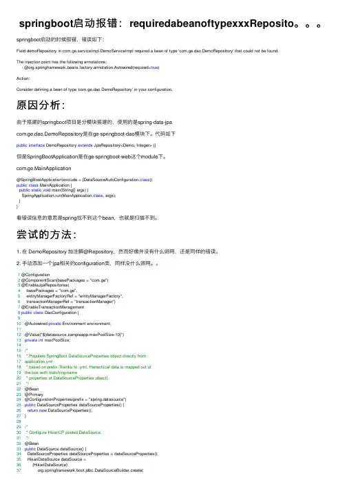
springboot启动报错:requiredabeanoftypexxxReposito。
springboot启动的时候报错,错误如下:Field demoRepository in com.ge.serviceImpl.DemoServiceImpl required a bean of type 'com.ge.dao.DemoRepository' that could not be found.The injection point has the following annotations:- @org.springframework.beans.factory.annotation.Autowired(required=true)Action:Consider defining a bean of type 'com.ge.dao.DemoRepository' in your configuration.原因分析:由于搭建的springboot项⽬是分模块搭建的,使⽤的是spring-data-jpacom.ge.dao.DemoRepository是在ge-springboot-dao模块下。
代码如下public interface DemoRepository extends JpaRepository<Demo, Integer> {}但是SpringBootApplication是在ge-springboot-web这个module下。
com.ge.MainApplication@SpringBootApplication(exclude = {DataSourceAutoConfiguration.class})public class MainApplication {public static void main(String[] args) {SpringApplication.run(MainApplication.class, args);}}看错误信息的意思是spring找不到这个bean,也就是扫描不到。
DataGridview Default Error DialogIntroductionThe DataGridview Default Error Dialog is a feature provided by the DataGridview control in various programming languages and frameworks, such as C#, , and Java. This error dialog is displayed when an error occurs during data validation or when an exception is thrown while processing data in the DataGridview.Understanding the DataGridview Default Error DialogThe DataGridview is a popular control used to display and manipulate tabular data in desktop applications. It allows users to edit, delete, and add rows of data. When the user modifies data in the DataGridview, such as entering an invalid value or leaving a required field empty, the control performs validation to ensure the data’s integrity.1. Triggering the Default Error DialogWhen a user enters invalid data or violates any validation rules, the DataGridview control triggers the Default Error Dialog. This dialog is displayed to notify the user about the error and provide options for handling it. The dialog typically contains an error message describing the problem, along with buttons to choose how to proceed.2. Customizing Error MessagesDevelopers can customize the error messages displayed in the Default Error Dialog. By handling the DataError event of the DataGridview, they can intercept and modify the default error message. This allows them to provide more meaningful and user-friendly messages, tailored to their application’s requirements.Benefits of the DataGridview Default Error DialogThe DataGridview Default Error Dialog offers several benefits to both developers and end-users.1. Improved User ExperienceBy displaying informative error messages, the Default Error Dialog helps users easily identify and understand the cause of an error. It explains what went wrong and guides them on how to rectify the issue. This enhances the overall user experience by reducing confusion and frustration.2. Simplified Error HandlingThe Default Error Dialog provides convenient options for handling errors. It typically includes buttons such as “Retry,” “Cancel,” or “Ignore,” allowing users to choose an appropriate action. This simplifies the error handling process, as users can decide whether to correct the error, cancel the operation, or ignore the error and proceed.3. Consistency in Error ReportingUsing the DataGridview Default Error Dialog ensures consistent error reporting throughout an application. Regardless of the type of error or exception, the dialog provides a standardized interface to present the error to the user. This consistency makes it easier for users to understand and respond to errors consistently across different parts of the application.Best Practices for Handling ErrorsWhen working with the DataGridview Default Error Dialog, developers should follow some best practices to ensure effective error handling and a smooth user experience.1. Validate Input DataTo minimize the occurrence of errors triggering the Default Error Dialog, developers should implement strong data validation mechanisms. This includes performing checks for required fields, data type validation, length validation, and any custom validation rules specific to the application’s domain.2. Provide Meaningful Error MessagesDefault error messages can sometimes be generic and not user-friendly. Developers should provide clear and meaningful error messages that describe the problem in plain language. This helps users understand the error and take appropriate action to rectify it.3. Offer Guidance for Error ResolutionIn addition to a descriptive error message, it is helpful to provide guidance on how to resolve the error. This can be done by suggesting possible solutions, providing hints, or offering links to relevant documentation or help resources.4. Handle Exceptions GracefullyThe DataGridview Default Error Dialog is often triggered by exceptions thrown during data processing. Developers should handle these exceptions gracefully by using try-catch blocks. Instead of relying solely on the Default Error Dialog, developers can catch the exception, log it for debugging purposes, and then display a custom error message to the user.ConclusionThe DataGridview Default Error Dialog is a valuable feature that enhances the usability and robustness of applications using the DataGridview control. It provides a consistent and user-friendly way to handle errors and exceptions encountered during data validation and processing. By following best practices and customizing error messages, developers can create an excellent user experience and simplify error handling in their applications.。
Package‘ncdump’October13,2022Title Extract Metadata from'NetCDF'Files as Data FramesVersion0.0.3Description Tools for handling'NetCDF'metadata in data frames.The metadata is provided as relations in tabular form,to avoid having to scan printed header output or to navigatenested lists of raw metadata.License GPL-3LazyData trueImports dplyr,ncdf4RoxygenNote6.0.1Suggests testthat,knitr,rmarkdown,covrURL https:///r-gris/ncdumpBugReports https:///r-gris/ncdump/issuesNeedsCompilation noAuthor Michael D.Sumner[aut,cre]Maintainer Michael D.Sumner<******************>Repository CRANDate/Publication2017-05-0212:35:30UTCR topics documented:ncdump (2)NetCDF (2)Index41ncdump ncdump for NetCDF metadata.DescriptionProvides a useable data structure of NetCDF metadata NetCDF is Network Common Data Form https:///software/netcdf/.DetailsThere is one main function:NetCDF produces a list of data frames containing metadata from a NetCDFfile NetCDF Information about a NetCDFfile,in convenient form.DescriptionNetCDF scans all the metadata provided by the ncdf4::nc_open function,and organizes it by the entities in thefile.UsageNetCDF(x)Argumentsx path to NetCDFfileDetailsUsers of’NetCDF’files might be familiar with the command line tool’ncdump-h’noting that the"header"argument is crucial for giving a compact summary of the contents of afile.This package aims to provide that information as data,to be used for writing code to otherwise access and manipulate the contents of thefiles.This function doesn’t do anything with the data,and it doesn’t access any of the data.A NetCDFfile contains the following entities,and each gets a data frame in the resulting object:attribute’attributes’are general metadata about thefile and its variables and dimensions dimension’dimensions’are the axes defining the space of the data variablesvariable’variables’are the actual data,the arrays containing data valuesgroup’groups’are an internal abstraction to behave as a collection,analogous to afile.In addition to a data for each of the main entities above’NetCDF’also creates:unlimdims the unlimited dimensions identify those which are not a constant lenghth(i.e.spread overfiles) dimvals a link table between dimensions and its coordinatesfile information about thefile itselfvardim a link table between variables and their dimensionsCurrently’file’is expected to and treated as having only one row,but future versions may treat acollection offiles as a single entity.The’ncdump-h’print summary above is analogous to the print method ncdf4::print.ncdf4of theoutput of ncdf4::nc_open.ValueA list of data frames with an unused S3class’NetCDF’,see details for a description of the dataframes.The’attribute’data frame has class’NetCDF_attributes’,this is used with a custom printmethod to reduce the amount of output printed.See Alsoncdf4::nc_open which is what this function uses to obtain the informationExamplesrnc<-NetCDF(system.file("extdata","S2008001.L3m_DAY_CHL_chlor_a_9km.nc",package="ncdump")) rncIndexncdf4::nc_open,2,3ncdf4::print.ncdf4,3ncdump,2ncdump-package(ncdump),2NetCDF,2,24。
bootstrapvalidator 动态修改规则-概述说明以及解释1.引言1.1 概述引言是文章的开头部分,用来对整篇文章进行一个简要概述,向读者介绍文章的主题和背景。
对于标题为"bootstrapvalidator 动态修改规则"的文章,可以在引言部分进行如下概述:引言部分旨在介绍本文将要讨论的内容——Bootstrap Validator动态修改规则。
在开发网页表单的过程中,常常会遇到需要根据用户的输入动态改变表单验证规则的需求。
在传统的表单验证方式中,一般是在表单初始化时就设置好了规则,但这种静态的验证规则不能满足动态的需求。
本文将首先简要介绍Bootstrap Validator的概念和基本使用方法,然后重点探讨在使用Bootstrap Validator时如何实现动态修改验证规则。
具体来说,将讨论如何根据用户的输入或其他外部条件,实现动态增加、删除、修改表单验证规则的功能。
通过本文的学习,读者将能够掌握如何灵活地使用Bootstrap Validator来满足网页表单动态验证的需求。
此外,现代网页应用中对表单验证的需求越来越复杂,而Bootstrap Validator作为一款强大而灵活的表单验证插件,将在未来的应用中有着广阔的发展前景。
接下来的章节中,我们将从简介和需求两个方面出发,详细介绍Bootstrap Validator和动态修改规则的需求,并提供实际的方法来实现这一功能。
最后,在结论部分将对本文进行总结,并展望Bootstrap Validator在表单验证领域的应用前景。
希望本文能够对读者对于Bootstrap Validator和动态修改规则有一个全面的了解,并能够为读者在网页表单验证的实践中提供一定的指导和帮助。
1.2文章结构文章结构:文章的整体结构分为引言、正文和结论三部分。
引言部分主要介绍了本篇文章的背景和目的。
在概述中,简要介绍了bootstrapvalidator的基本概念和作用。
Bootstrap Moran's Ⅰ Test of Spatial Panel Data
Model
作者: 龙志和[1];李伟杰[1]
作者机构: [1]华南理工大学
出版物刊名: 统计研究
页码: 97-101页
年卷期: 2014年 第9期
主题词: Bootstrap抽样;Moran's;Ⅰ检验;空间面板数据;Monte;Carlo模拟
摘要:误差项不服从经典假设时,空间面板数据模型的Moran's Ⅰ检验存在较大的水平扭曲,导致空间相关性检验失效.本文采用改进的Bootstrap抽样方法,对空间面板数据模型的Moran's Ⅰ检验进行优化.蒙特卡洛模拟结果表明,在误差项正态分布条件下,渐近Moran's Ⅰ检验和Bootstrap Moran's Ⅰ检验均具有较优越的检验水平和检验功效表现;在误差项时间序列相关条件下,渐近Moran's Ⅰ检验存在严重的水平扭曲,而Bootstrap Moran's Ⅰ检验能够有效地矫正水平扭曲,且检验功效优于渐近Moran's Ⅰ检验,是更为有效的检验统计量.。
雾霾污染对服务业绿色发展的影响研究雾霾污染对服务业绿色发展的影响研究----基于省级面板数据的空间计量经济学实证赵军峰叫冉启英Z(1.新疆大学经济与管理学院,新疆乌鲁木齐830046;2.重庆工商大学环境与资源学院,重庆400067;3.新疆大学创新管理研究中心,新疆乌鲁木齐830046)摘要:运用非径向距离函数(NDDF)测算出2006—2016年中国30个(西藏、港澳台除外)省区市的服务业绿色发展水平,构建了地理距离矩阵、经济距离矩阵和技术距离矩阵,对比分析了雾霾污染对省份服务业绿色发展水平的全局性和异质性影响。
研究发现:雾霾污染与省份服务业绿色发展水平之间存在此消彼长的关系,雾霾污染与省份服务业绿色发展水平在全国层面可能存在“N型”关系,而与人力资本存在较弱的“倒N型”关系,雾霾污染与东部省份服务业绿色发展水平可能存在“倒U 型”曲线关系,而与中部省份、西部省区市服务业绿色水平存在“U型”曲线关系。
研究从雾霾治理政策、研发投入强度、基础设施建设力度等方面提出相应对策建议。
关键词:雾霾污染;月艮务业;距离矩阵;绿色协调;创新能力中图分类号:F719文献标识码:A文章编号:1004-292X(2021)04-0089-06Research on the Impact of Haze Pollution on the Green Development of Service Industry: An Empirical Study of Spatial Econometrics based on Provincial Panel DataZHAO Jun-feng1,2,RAN Qi-ying1,3(1.School of Economics and Management,Xinjiang University,Urumqi Xinjiang830046,China;2.College of Environment and Resources,Chongqing Technology and Business University,Chongqing400067,China;3.Center for Innovation Management Research,Xinjiang University,Urumqi Xinjiang830046,China)Abstract:The paper uses the non radial distance function(NDDF)to calculate the level of green development of service industry in30provinces(cities)of China(except Tibet,Hong Kong,Macao and Taiwan)from2006to2016,and comparatively analyzes the global and heterogeneous impact of haze pollution on the green development of service industry in provinces by constructing the geographical distance matrix,economic distance matrix and technical distance matrix.The results show that:Haze pollution and the green development of service industry in provinces have a reciprocal relationship,and they may have a"N-type"relationship at the national level, while there is a weak"inverted N-type"relationship between haze pollution and human capital.Haze pollution and the green development of service industry in eastern provinces may have an"inverted U-type"curve relationship,while they have a"U-shaped"curve relationship in central and western provinces.Therefore,suggestions are put forward from the aspects of haze control policy,R&D investment intensity,infrastructure construction.Key words:Haze pollution;Service industry;Distance matrix;Green and coordinated development;Innovative ability一、引言目的成就,尤其是中国服务业得到了长足发展。