Towards a Tool for Performance Evaluation of Autonomous Vehicle Navigation in Dynamic, On-R

The evolution of the automobile has been a fascinating journey,reflecting not just technological advancements but also the changing needs and desires of society.From the early days of the horseless carriage to the modern selfdriving vehicles,the automobile has undergone significant transformations.Lets delve into the history and development of the automobile in English,exploring its impact on culture,the economy,and the environment.The Dawn of the Automobile EraThe first automobiles were a far cry from the sleek machines we know today.The invention of the automobile is often attributed to Karl Benz,who patented the first gasolinepowered vehicle in1885.However,the concept of a selfpropelled vehicle had been around for centuries,with early versions powered by steam or electricity.The Rise of Mass ProductionThe real turning point in automobile history came with the introduction of the assembly line by Henry Ford in1913.This innovation allowed for the mass production of cars, making them affordable for the average American.Fords Model T was a gamechanger, democratizing automobile ownership and paving the way for the modern automotive industry.The PostWar BoomAfter World War II,the automobile industry experienced a boom.With the economy recovering and a growing middle class,there was a surge in demand for personal vehicles. Car manufacturers began to diversify their offerings,introducing new models and designs that catered to different tastes and needs.The Environmental ImpactAs the number of cars on the road increased,so did the environmental impact.The rise in automobile use led to increased air pollution and contributed to climate change.This prompted a shift in focus towards more sustainable transportation solutions,with the development of electric and hybrid vehicles.The Digital RevolutionThe advent of digital technology has revolutionized the automobile industry.Modern cars are equipped with advanced electronics,offering features like GPS navigation, infotainment systems,and even driver assistance technologies.The integration ofsmartphones with vehicle systems has further enhanced the driving experience.The Future of AutomobilesThe future of the automobile is being shaped by the pursuit of sustainability and the integration of artificial intelligence.Electric vehicles EVs are becoming more prevalent, with companies like Tesla leading the charge.Autonomous vehicles,or selfdriving cars, are another exciting development,promising to change the way we travel and interact with our surroundings.ConclusionThe automobile has come a long way since its inception,and its development is a testament to human ingenuity and the desire for progress.As we look to the future,the automobile industry continues to innovate,responding to the challenges of the environment,safety,and the need for more personalized transportation solutions.The journey of the automobile is far from over,and its next chapter promises to be just as exciting as its past.。

Ultrasonic ranging system designPublication title: Sensor Review. Bradford: 1993.Vol.ABSTRACT: Ultrasonic ranging technology has wide using worth in many fields, such as the industrial locale, vehicle navigation and sonar engineering. Now it has been used in level measurement, self-guided autonomous vehicles, fieldwork robots automotive navigation, air and underwater target detection, identification, location and so on. So there is an important practicing meaning to learn the ranging theory and ways deeply. To improve the precision of the ultrasonic ranging system in hand, satisfy the request of the engineering personnel for the ranging precision, the bound and the usage, a portable ultrasonic ranging system based on the single chip processor was developed.Keywords: Ultrasound, Ranging System, Single Chip Processor1. IntroductiveWith the development of science and technology, the improvement of people’s standard of living, speeding up the development and construction of the city. Urban drainage system have greatly developed their situation is construction improving. However, due to historical reasons many unpredictable factors in the synthesis of her time, the city drainage system. In particular drainage system often lags behind urban construction. Therefore, there are often good building excavation has been building facilities to upgrade the drainage system phenomenon. It brought to the city sewage, and it is clear to the city sewage and drainage culvert in the sewage treatment system.Co mfort is very important to people’s lives. Mobile robots designed to clear the drainage culvert and the automatic control system Free sewage culvert clear guarantee robots, the robot is designed to clear the culvert sewage to the core. Control system is the core component of the development of ultrasonic range finder. Therefore, it is very important to design a good ultrasonic range finder.2. A principle of ultrasonic distance measurementThe application of AT89C51:SCM is a major piece of computer components are integrated into the chip micro-computer. It is a multi-interface and counting on the micro-controller integration, and intelligence products are widely used in industrial automation. and MCS-51 microcontroller is a typical and representative.Microcontrollers are used in a multitude of commercial applications such as modems, motor-control systems, air conditioner control systems, automotive engine and among others. The high processing speed and enhanced peripheral set of these microcontrollers make them suitable for such high-speed event-based applications. However, these critical application domains also require that these microcontrollers are highly reliable. The high reliability and low market risks can be ensured by a robust testing process and a proper tools environment for the validation of these microcontrollers both at the component and at the system level. Intel Plaform Engineering department developed an object-oriented multi-threaded test environment for the validation of its AT89C51 automotive microcontrollers. The goals of this environment was not only to provide a robust testing environment for the AT89C51 automotive microcontrollers, but to develop an environment which can be easily extended and reused for the validation of several other future microcontrollers. The environment was developed in conjunction with Microsoft Foundation Classes(AT89C51).1.1 Features* Compatible with MCS-51 Products* 2Kbytes of Reprogrammable Flash MemoryEndurance: 1,000Write/Erase Cycles* 2.7V to 6V Operating Range* Fully Static operation: 0Hz to 24MHz* Two-level program memory lock* 128x8-bit internal RAM* 15programmable I/O lines* Two 16-bit timer/counters* Six interrupt sources*Programmable serial UART channel* Direct LED drive output* On-chip analog comparator* Low power idle and power down modes1.2 DescriptionThe AT89C2051 is a low-voltage, high-performance CMOS 8-bit microcomputer with 2Kbytes of flash programmable and erasable read only memory (PEROM). The device is manufactured using Atmel’s high density nonvolatile memory technology and is compatible with the industry standard MCS-51 instruction set and pinout. By combining a versatile 8-bit CPU with flash on a monolithic chip, the Atmel AT89C2051 is a powerful microcomputer which provides a highly flexible and cost effective solution to many embedded control applications.The AT89C2051 provides the following standard features: 2Kbytes of flash,128bytes of RAM, 15 I/O lines, two 16-bit timer/counters, a five vector two-level interrupt architecture, a full duplex serial port, a precision analog comparator, on-chip oscillator and clock circuitry. In addition, the AT89C2051 is designed with static logicfor operation down to zero frequency and supports two software selectable power saving modes. The idle mode stops the CPU while allowing the RAM, timer/counters, serial port and interrupt system to continue functioning. The power down mode saves the RAM contents but freezer the oscillator disabling all other chip functions until the next hardware reset.1.3 Pin Configuration1.4 Pin DescriptionVCC Supply voltage.GND Ground.Prot 1Prot 1 is an 8-bit bidirectional I/O port. Port pins P1.2 to P1.7 provide internal pullups. P1.0 and P1.1 require external pullups. P1.0 and P1.1 also serve as the positive input (AIN0) and the negative input (AIN1), respectively, of the on-chip precision analog comparator. The port 1 output buffers can sink 20mA and can drive LED displays directly. When 1s are written to port 1 pins, they can be used as inputs. When pins P1.2 to P1.7 are used as input and are externally pulled low, they will source current (IIL) because of the internal pullups.Port 3Port 3 pins P3.0 to P3.5, P3.7 are seven bidirectional I/O pins with internal pullups. P3.6 is hard-wired as an input to the output of the on-chip comparator and is not accessible as a general purpose I/O pin. The port 3 output buffers can sink 20mA. When 1s are written to port 3 pins they are pulled high by the internal pullups and can be used as inputs. As inputs, port 3 pins that are externally being pulled low will source current (IIL) because of the pullups.Port 3 also serves the functions of various special features of the AT89C2051 as listed below.1.5 Programming the FlashThe AT89C2051 is shipped with the 2 Kbytes of on-chip PEROM code memory array in the erased state (i.e., contents=FFH) and ready to be programmed. The code memory array is programmed one byte at a time. Once the array is programmed, to re-program any non-blank byte, the entire memory array needs to be erased electrically.Internal address counter: the AT89C2051 contains an internal PEROM address counter which is always reset to 000H on the rising edge of RST and is advanced applying a positive going pulse to pin XTAL1.Programming algorithm: to program the AT89C2051, the following sequence is recommended.1. power-up sequence:Apply power between VCC and GND pins Set RST and XTAL1 to GNDWith all other pins floating , wait for greater than 10 milliseconds2. Set pin RST to ‘H’ set pin P3.2 to ‘H’3. Apply the appropriate combination of ‘H’ or ‘L’ logic to pins P3.3, P3.4, P3.5,P3.7 to select one of the programming operations shown in the PEROM programming modes table.To program and Verify the Array:4. Apply data for code byte at location 000H to P1.0 to P1.7.5.Raise RST to 12V to enable programming.5. Pulse P3.2 once to program a byte in the PEROM array or the lock bits. The byte-write cycle is self-timed and typically takes 1.2ms.6. To verify the programmed data, lower RST from 12V to logic ‘H’ level and set pins P3.3 to P3.7 to the appropriate levels. Output data can be read at the port P1 pins.7. To program a byte at the next address location, pulse XTAL1 pin once to advance the internal address counter. Apply new data to the port P1 pins.8. Repeat steps 5 through 8, changing data and advancing the address counter for the entire 2 Kbytes array or until the end of the object file is reached.9. Power-off sequence: set XTAL1 to ‘L’ set RST to ‘L’Float all other I/O pins Turn VCC power off2.1 The principle of piezoelectric ultrasonic generatorPiezoelectric ultrasonic generator is the use of piezoelectric crystal resonators to work. Ultrasonic generator, the internal structure as shown, it has two piezoelectric chip and a resonance plate. When it’s two plus pulse signal, the frequency equal to the intrinsic piezoelectric oscillation frequency chip, the chip will happen piezoelectric resonance, and promote the development of plate vibration resonance, ultrasound is generated. Conversely, it will be for vibration suppression of piezoelectric chip, the mechanical energy is converted to electrical signals, then it becomes the ultrasonic receiver.The traditional way to determine the moment of the echo’s arrival is based on thresholding the received signal with a fixed reference. The threshold is chosen well above the noise level, whereas the moment of arrival of an echo is defined as the first moment the echo signal surpasses that threshold. The intensity of an echo reflecting from an object strongly depends on the object’s nature, size and distance from the sensor. Further, the time interval from the echo’s starting point to the moment when it surpasses the threshold changes with the intensity of the echo. As a consequence, a considerable error may occur even two echoes with different intensities arriving exactly at the same time will surpass the threshold at different moments. The stronger one will surpass the threshold earlier than the weaker, so it will be considered as belonging to a nearer object.2.2 The principle of ultrasonic distance measurementUltrasonic transmitter in a direction to launch ultrasound, in the moment to launch the beginning of time at the same time, the spread of ultrasound in the air, obstacles on his way to return immediately, the ultrasonic reflected wave received by the receiverimmediately stop the clock. Ultrasound in the air as the propagation velocity of 340m/s, according to the timer records the time t, we can calculate the distance between the launch distance barrier(s), that is: s=340t / 23. Ultrasonic Ranging System for the Second Circuit DesignSystem is characterized by single-chip microcomputer to control the use of ultrasonic transmitter and ultrasonic receiver since the launch from time to time, single-chip selection of 875, economic-to-use, and the chip has 4K of ROM, to facilitate programming.3.1 40 kHz ultrasonic pulse generated with the launchRanging system using the ultrasonic sensor of piezoelectric ceramic sensorsUCM40, its operating voltage of the pulse signal is 40kHz, which by the single-chip implementation of the following procedures to generate.puzel: mov 14h, # 12h; ultrasonic firing continued 200msHere: cpl p1.0; output 40kHz square wavenop;nop;nop;djnz 14h, here;retRanging in front of single-chip termination circuit P1.0 input port, single chip implementation of the above procedure, the P1.0 port in a 40kHz pulse output signal, after amplification transistor T, the drive to launch the first ultrasonic UCM40T, issued 40kHz ultrasonic pulse, and the continued launch of 200ms. Ranging the right and the left side of the circuit, respectively, then input port P1.1 and P1.2, the working principle and circuit in front of the same location.3.2 Reception and processing of ultrasonicUsed to receive the first launch of the first pair UCM40R, the ultrasonic pulse modulation signal into an alternating voltage, the op-amp amplification IC1A and after polarization IC1B to IC2. IC2 is locked loop with audio decoder chip LM567, internal voltage-controlled oscillator center frequency of f0=1/1.1R8C3, capacitor C4 determinetheir target bandwidth. R8-conditioning in the launch of the high jump 8 feet into a low-level, as interrupt request signals to the single-chip processing.Ranging in front of single-chip termination circuit output port INT0 interrupt the highest priority, right or left location of the output circuit with output gate IC3A access INT1 port single-chip, while single-chip P1.3 and P1.4 received input IC3A, interrupted by the process to identify the source of inquiry to deal with, interrupt priority level for the first left right after. Part of the source code is as follows:Receivel: push pswpush accclr ex1; related external interrupt 1jnb p1.1, right; P1.1 pin to 0, ranging from right to interrupt service routine circuitjnb p1.2, left; P1.2 pin to 0, to the left ranging circuit interrupt service routinereturn: SETB EX1; open external interrupt 1pop accpop pswretiright: …; right location entrance circuit interrupt service routineAjmp Returnleft: …; left ranging entrance circuit interrupt service routineAjmp Return3.3 The calculation of ultrasonic propagation timeWhen you start firing at the same time start the single-chip circuitry within the timer T0, the use of timer counting function records the time and the launch of ultrasonic reflected wave received time. When you receive the ultrasonic reflected wave, the receiver circuit output a negative jump in the end of INT0 or INT1 interrupt request generates a signal, single-chip microcomputer in response to external interrupt request, the implementation of the external interrupt service subroutine, read the time difference, calculating the distance. Some of its source code is as follows:RECEIVE0: PUSH PSWPUSH ACCCLR EX0; related external interrupt 0MOV R7, TH0; read the time valueMOV R6, TL0CLR CMOV A, R6SUBB A, #0BBH; calculate the time differenceMOV 31H, A; storage resultsMOV A, R7SUBB A, # 3CHMOV 30H, ASETB EX0; open external interrupt 0\POP ACCPOP PSWRETIFor a flat target, a distance measurement consists of two phases: a coarse measurement and a fine measurement:Step 1: Transmission of one pulse train to produce a simple ultrasonic wave.Step 2: Changing the gain of both echo amplifiers according to equation, until the echo is detected.Step 3: Detection of the amplitudes and zero-crossing times of both echoes.Step 4: Setting the gains of both echo amplifiers to normalize the output at, say 3 volts. Setting the period of the next pulses according to the: period of echoes. Setting the time window according to the data of step 2.Step 5: Sending two pulse trains to produce an interfered wave. Testing the zero-crossing times and amplitudes of the echoes. If phase inversion occurs in the echo, determine to otherwise calculate to by interpolation using the amplitudes near the trough. Derive t sub m1 and t sub m2.Step 6: Calculation of the distance y using equation.4、The ultrasonic ranging system software designSoftware is divided into two parts, the main program and interrupt service routine. Completion of the work of the main program is initialized, each sequence of ultrasonic transmitting and receiving control.Interrupt service routines from time to time to complete three of the rotation direction of ultrasonic launch, the main external interrupt service subroutine to read the value of completion time, distance calculation, the results of the output and so on.5、ConclusionsRequired measuring range of 30cm-200cm objects inside the plane to do a number of measurements found that the maximum error is 0.5cm, and good reproducibility. Single-chip design can be seen on the ultrasonic ranging system has a hardware structure is simple, reliable, small features such as measurement error. Therefore, it can be used not only for mobile robot can be used in other detection system.Thoughts: As for why the receiver do not have the transistor amplifier circuit, because the magnification well, integrated amplifier, but also with automatic gain control level, magnification to 76dB, the center frequency is 38k to 40k, is exactly resonant ultrasonic sensors frequency.6、Parking sensor6.1 Parking sensor introductionReversing radar, full name is "reversing the anti-collision radar, also known as" parking assist device, car parking or reversing the safety of assistive devices, ultrasonic sensors(commonly known as probes), controls and displays (or buzzer)and other components. To inform the driver around the obstacle to the sound or a moreintuitive display to lift the driver parking, reversing and start the vehicle around tovisit the distress caused by, and to help the driver to remove the vision deadends and blurred vision defects and improve driving safety.6.2 Reversing radar detection principleReversing radar, according to high-speed flight of the bats in thenight, not collided with any obstacle principles of design anddevelopment. Probe mounted on the rear bumper, according to different price and brand, the probe only ranging from two, three, four, six, eight,respectively, pipe around. The probe radiation, 45-degree angle up and downabout the search target. The greatest advantage is to explore lower than the bumper of the driver from the rear window is difficult to see obstacles, and the police, suchas flower beds, children playing in the squatting on the car.Display parking sensor installed in the rear view mirror, it constantlyremind drivers to car distance behindthe object distance to the dangerous distance, the buzzer starts singing, allow the driver to stop. When the gear lever linked into reverse gear, reversing radar, auto-start the work, the working range of 0.3 to 2.0 meters, so stop when the driver was very practical. Reversing radar is equivalent to an ultrasound probe for ultrasonic probe can be divided into two categories: First, Electrical, ultrasonic, the second is to use mechanical means to produce ultrasound, in view of the more commonly used piezoelectric ultrasonic generator, it has two power chips and a soundingboard, plus apulse signal when the poles, its frequency equal to the intrinsic oscillation frequency of the piezoelectric pressure chip will be resonant and drivenby the vibration of the sounding board, the mechanical energy into electrical signal, which became the ultrasonic probe works. In order to better study Ultrasonic and use up, people have to design and manufacture of ultrasonic sound, the ultrasonic probe tobe used in the use of car parking sensor. With this principle in a non-contactdetection technology for distance measurement is simple, convenient and rapid, easyto do real-time control, distance accuracy of practical industrial requirements. Parking sensor for ranging send out ultrasonic signal at a givenmoment, and shot in the face of the measured object back to the signal wave, reversing radar receiver to use statistics in the ultrasonic signal from the transmitter to receive echo signals calculate the propagation velocity in the medium, which can calculate the distance of the probe and to detect objects.6.3 Reversing radar functionality and performanceParking sensor can be divided into the LCD distance display, audible alarm, and azimuth directions, voice prompts, automatic probe detection function is complete, reversing radar distance, audible alarm, position-indicating function. A good performance reversing radar, its main properties include: (1) sensitivity, whether theresponse fast enough when there is an obstacle. (2) the existence of blind spots. (3) detection distance range.6.4 Each part of the roleReversing radar has the following effects: (1) ultrasonic sensor: used tolaunch and receive ultrasonic signals, ultrasonic sensors canmeasure distance. (2) host: after the launch of the sine wave pulse to the ultrasonic sensors, and process the received signal, to calculate the distance value, the data and monitor communication. (3) display or abuzzer: the receivinghost from the data, and display the distance value and provide differentlevels according to the distance from the alarm sound.6.5 Cautions1, the installation height: general ground: car before the installation of 45 ~55: 50 ~ 65cmcar after installation. 2, regular cleaningof the probe to prevent the fill. 3, do not use the hardstuff the probe surface cover will produce false positives or ranging allowed toprobe surface coverage, such as mud. 4, winter to avoid freezing. 5, 6 / 8 probe reversing radar before and after the probe is not free to swap may cause the ChangMing false positive problem. 6, note that the probe mounting orientation, in accordance with UP installation upward. 7, the probe is not recommended to install sheetmetal, sheet metal vibration will cause the probe resonance, resulting in false positives.超声测距系统设计原文出处：传感器文摘布拉福德：1993年超声测距技术在工业现场、车辆导航、水声工程等领域具有广泛的应用价值，目前已应用于物位测量、机器人自动导航以及空气中与水下的目标探测、识别、定位等场合。

IntroductionTransportation vehicles, the lifeblood of modern societies, play an indispensable role in facilitating the movement of people, goods, and services across vast geographical landscapes. Their quality and adherence to high standards are crucial determinants of their overall efficiency, safety, environmental impact, and user satisfaction. This comprehensive analysis delves into multiple aspects of transportation vehicles, examining their design, technology, sustainability, safety features, and regulatory frameworks, all of which contribute to their overall quality and adherence to stringent standards.1. Design and Engineering ExcellenceThe quality of a transportation vehicle begins with its design and engineering. High-quality vehicles are meticulously crafted to ensure optimal performance, reliability, and longevity. This involves the use of advanced materials, such as lightweight yet durable alloys and composites, which reduce weight without compromising structural integrity, thereby improving fuel efficiency and reducing emissions. Additionally, aerodynamic designs minimize air resistance, further enhancing fuel economy and overall performance.Sophisticated powertrains, including electric, hybrid, and highly efficient internal combustion engines, demonstrate technological prowess and commitment to reducing environmental impact. Moreover, ergonomic interiors, designed with user comfort and accessibility in mind, contribute to the overall passenger experience. Advanced noise, vibration, and harshness (NVH) control technologies ensure a quiet, smooth ride, further enhancing the perceived quality of the vehicle.2. Technological Advancements and IntegrationIn the era of digitalization and connectivity, the integration of cutting-edge technology is a hallmark of high-quality transportation vehicles. Infotainment systems with intuitive interfaces, smartphone integration, and advanced navigation capabilities provide passengers with seamless access to information and entertainment. Furthermore, telematics systems enable real-time monitoring of vehicle performance, predictive maintenance, and remote diagnostics, ensuring optimal operation and reducing downtime.Autonomous driving technologies, including sensors, cameras, radar, and LiDAR, coupled with sophisticated artificial intelligence algorithms, promise enhanced safety, efficiency, and convenience. Advanced driver assistance systems (ADAS), such as adaptive cruise control, lane departure warning, and automatic emergency braking, not only enhance safety but also serve as stepping stones towards fully autonomous vehicles.3. Environmental Sustainability and Energy EfficiencyQuality in contemporary transportation vehicles is increasingly linked to their environmental sustainability and energy efficiency. The shift towards electric vehicles (EVs), plug-in hybrids (PHEVs), and hydrogen fuel cell vehicles (FCVs) reflects a commitment to reducing greenhouse gas emissions and mitigating climate change. These vehicles offer zero or low tailpipe emissions,reduced dependence on fossil fuels, and improved overall energy efficiency compared to traditional internal combustion engine vehicles.Moreover, advancements in battery technology, such as higher energy density, faster charging times, and longer lifespans, are enhancing the practicality and appeal of EVs. The development of robust charging infrastructure and policies promoting the adoption of clean vehicles further contribute to the quality of the overall transportation ecosystem.4. Safety Features and Standards ComplianceSafety is an absolute imperative in assessing the quality of any transportation vehicle. High-quality vehicles incorporate a range of passive and active safety features designed to prevent accidents, protect occupants in the event of a collision, and mitigate potential hazards.Passive safety features include strong crash-resistant structures, crumple zones, airbags, and seat belt systems that work together to minimize injury during an accident. Active safety features, such as electronic stability control, anti-lock braking systems, and ADAS mentioned earlier, help drivers avoid accidents altogether.Stringent adherence to international safety standards, such as those set by the European New Car Assessment Programme (Euro NCAP), the Insurance Institute for Highway Safety (IIHS) in the United States, and the United Nations Economic Commission for Europe (UNECE) regulations, ensures that vehicles meet or exceed globally recognized benchmarks for occupant protection, pedestrian safety, and crashworthiness.5. Regulatory Frameworks and Quality ControlThe quality of transportation vehicles is also influenced by the regulatory frameworks within which they are designed, manufactured, and operated. Governments and international organizations establish and enforce rigorous standards and regulations covering aspects such as emissions, fuel efficiency, safety, noise, and recyclability. Compliance with these standards is closely monitored through testing, certification, and periodic inspections.Manufacturers themselves implement stringent quality control processes throughout the supply chain, from raw material sourcing to final assembly, to ensure consistent product quality. Lean manufacturing principles, Six Sigma methodologies, and continuous improvement initiatives help identify and rectify defects, minimize waste, and enhance overall production efficiency.ConclusionIn summary, the quality of transportation vehicles is a multifaceted concept encompassing design excellence, technological innovation, environmental sustainability, safety features, and adherence to rigorous standards and regulations. As society continues to evolve, so too will the expectations and definitions of quality in transportation vehicles. Future advancements in materials science, powertrain technology, autonomous systems, and renewable energy will undoubtedly shape the next generation of high-quality, standard-compliant transportation solutions, further enhancing mobility,safety, and environmental stewardship on a global scale.。

未来汽车发展趋势英语作文全文共3篇示例，供读者参考篇1Title: Future Trends in Automotive IndustryWith rapid advancements in technology and changing consumer preferences, the automotive industry is undergoing a major transformation. The future of automobiles is likely to be very different from what we see today, with an emphasis on sustainability, connectivity, and autonomous driving. In this essay, we will explore some of the key trends that are shaping the future of the automotive industry.One of the most significant trends in the automotive industry is the shift towards electric vehicles (EVs). With concerns about climate change and air pollution on the rise, governments around the world are introducing stricter emissions regulations, prompting automakers to invest heavily in electric vehicle technology. EVs offer a cleaner and more sustainable alternative to traditional vehicles powered by internal combustion engines, and as battery technology improves and charging infrastructurebecomes more widespread, EVs are becoming increasingly popular among consumers.Along with the rise of electric vehicles, there is also a growing focus on autonomous driving technology. Self-driving cars have the potential to make roads safer, reduce traffic congestion, and provide greater mobility for people who are unable to drive themselves. Automakers and tech companies are investing billions of dollars in developing autonomous vehicle technology, and it is only a matter of time before self-driving cars become a common sight on our roads.Another key trend in the automotive industry is the increasing connectivity of vehicles. With the advent of the Internet of Things (IoT), cars are becoming more connected than ever before, allowing them to communicate with each other, with infrastructure such as traffic lights and road signs, and with other devices such as smartphones and smart home systems. Connected cars offer a range of benefits, including improved safety, enhanced entertainment options, and more efficient navigation.In addition to these technological advances, the future of the automotive industry is also likely to be shaped by changing consumer preferences. Millennial and Generation Z consumers,in particular, are more environmentally conscious and tech-savvy than previous generations, leading to a greater demand for electric vehicles, autonomous driving technology, and connected car features. Automakers will need to adapt to these changing preferences in order to stay competitive in the market.Overall, the future of the automotive industry is likely to be characterized by electric vehicles, autonomous driving technology, and connected cars. As technology continues to advance and consumer preferences evolve, automakers will need to innovate and adapt in order to thrive in the rapidly changing automotive landscape. The future of automobiles promises to be exciting, with new possibilities and opportunities for drivers and manufacturers alike.篇2The Future Trends of Automobile DevelopmentWith the rapid advancement of technology and the increasing focus on environmental sustainability, the automotive industry is undergoing significant changes. The future of automobiles is predicted to be vastly different from what we know today, with a shift towards electric vehicles, autonomousdriving, and connected cars. In this essay, we will explore the key trends shaping the future of automobile development.1. Electric Vehicles (EVs)One of the most significant trends in the automotive industry is the rise of electric vehicles. As concerns about climate change and air pollution grow, more and more consumers are looking for alternatives to traditional gasoline-powered cars. EVs offer a cleaner and more sustainable option, with zero emissions and lower operating costs. Major car manufacturers like Tesla, Nissan, and BMW are investing heavily in electric vehicle technology, leading to the development of more affordable and efficient EVs. The increasing availability of charging infrastructure and government incentives for EV adoption are also driving the growth of the electric vehicle market.2. Autonomous DrivingAnother major trend in automobile development is the advancement of autonomous driving technology. Self-driving cars have the potential to revolutionize the way we travel, offering enhanced safety, convenience, and efficiency. Companies like Google, Tesla, and Uber are investing in autonomous vehicle research and development, with the goal of achieving fully autonomous cars in the near future. While thereare still technical and regulatory challenges to overcome, the potential benefits of autonomous driving are driving significant investment and innovation in the automotive industry.3. Connected CarsIn addition to electric and autonomous vehicles, connected cars are also shaping the future of automobile development. Connected cars are equipped with advanced communication and connectivity features, allowing them to communicate with other vehicles, infrastructure, and devices. This enables a wide range of services and applications, such as real-time traffic information, remote diagnostics, and in-car entertainment. The emergence of 5G technology and the Internet of Things (IoT) are further driving the development of connected cars, with major car manufacturers like Ford, General Motors, and Volkswagen integrating connected car features into their vehicles.4. Sustainability and Environmental ConcernsAs concerns about climate change and environmental sustainability continue to grow, the automotive industry is under increasing pressure to reduce its carbon footprint. The shift towards electric vehicles is one of the key strategies for achieving this goal, as EVs produce zero emissions and have lowerlife-cycle carbon emissions compared to gasoline-powered cars.In addition to electric vehicles, car manufacturers are also exploring other sustainable technologies, such as hydrogen fuel cells, biofuels, and lightweight materials, to reduce the environmental impact of their vehicles. Governments around the world are also implementing stricter emissions regulations and incentives for eco-friendly vehicles, further driving the adoption of sustainable technologies in the automotive industry.5. Mobility as a Service (MaaS)Another important trend in automobile development is the concept of Mobility as a Service (MaaS). MaaS is a new approach to transportation that aims to provide seamless and integrated mobility solutions, combining public transport, shared mobility services, and on-demand transportation. Companies like Uber, Lyft, and Didi Chuxing are leading the way in the development of MaaS platforms, offering users a convenient and cost-effective alternative to car ownership. MaaS has the potential to reduce traffic congestion, improve air quality, and enhance the overall efficiency of transportation systems. As more people embrace shared mobility and on-demand services, the automotive industry is likely to see a shift towards more sustainable and flexible modes of transportation.In conclusion, the future of automobile development is shaping up to be electric, autonomous, connected, sustainable, and integrated. The rise of electric vehicles, autonomous driving technology, connected cars, sustainability initiatives, and Mobility as a Service are driving significant changes in the automotive industry. As car manufacturers, technology companies, and policymakers work together to address the challenges and opportunities of the future, we can expect to see a more efficient, sustainable, and interconnected transportation ecosystem in the years to come.篇3Title: Future Trends in Automotive DevelopmentThe automotive industry has been evolving rapidly over the past few years, with new technologies and innovative concepts changing the way we drive and interact with our vehicles. As we look to the future, there are several key trends that will shape the development of automobiles in the coming years.One of the most significant trends in automotive development is the shift towards electric vehicles (EVs). With growing concerns about climate change and the need to reduce emissions, many car manufacturers are investing heavily in theproduction of EVs. Governments around the world are also implementing policies to encourage the adoption of electric vehicles, such as tax incentives and stricter emissions standards. As a result, the market for EVs is expected to grow exponentially in the coming years.Another important trend in automotive development is the integration of autonomous driving technologies. Self-driving cars use a combination of sensors, cameras, and artificial intelligence to navigate the roads without human intervention. While fully autonomous vehicles are still in the testing phase, many car manufacturers are already incorporatingsemi-autonomous features into their vehicles, such as adaptive cruise control and lane-keeping assist. As these technologies continue to improve, we can expect to see more fully autonomous vehicles on the roads in the near future.In addition to electric and autonomous vehicles, the automotive industry is also seeing advancements in connectivity and digitalization. Many new cars are equipped with advanced infotainment systems that allow drivers to access maps, music, and other features from their smartphones. Some vehicles also have built-in internet connectivity, allowing for real-time updates and remote diagnostics. As the Internet of Things (IoT) continuesto grow, we can expect cars to become even more connected and integrated with other devices and services.Furthermore, sustainability is a key focus in the future development of automobiles. Car manufacturers are increasingly looking for ways to reduce the environmental impact of their vehicles, from using recycled materials in construction to implementing more efficient manufacturing processes. Some companies are also exploring alternative fuel sources, such as hydrogen fuel cells and biofuels, as a way to reduce carbon emissions and reliance on fossil fuels. By prioritizing sustainability, car manufacturers can meet the growing demand for environmentally friendly vehicles while also reducing their own carbon footprint.In conclusion, the future of automotive development is bright, with new technologies and concepts shaping the industry in exciting ways. From electric vehicles and autonomous driving to connectivity and sustainability, car manufacturers are continuously pushing the boundaries of innovation to create vehicles that are safer, more efficient, and more environmentally friendly. As we look ahead, it is clear that the automotive industry will continue to evolve and adapt to meet the changing needs of consumers and society as a whole.。

激光雷达英语专业术语English Answer:LiDAR (Light Detection and Ranging)。

LiDAR is a remote sensing technology that uses light in the form of a pulsed laser to measure ranges (variable distances) to the Earth. These light pulses – emitted from a rapidly firing laser – interact with the surface of the Earth and are scattered in different directions. The timeit takes for the reflected light to return to the sensor is recorded and used to calculate the distance between the sensor and the target. By emitting multiple laser pulses in rapid succession and scanning the pulses over a target area, a dense point cloud of the target can be generated.Key Components of a LiDAR System.Laser Source: Emits pulsed laser light at a specific wavelength.Scanner: Directs the laser pulses towards the target area.Detector: Receives the reflected laser pulses and measures the time-of-flight (TOF).Processing Unit: Computes the distances from the TOF measurements and generates a point cloud.Applications of LiDAR.LiDAR technology has numerous applications in various fields, including:Mapping and Surveying: Generating detailed terrain models, topographic maps, and bathymetric charts.Forestry: Estimating tree height, canopy cover, and biomass.Transportation: Autonomous vehicle navigation, roadmapping, and traffic monitoring.Archaeology: Discovering and mapping buried structures and artifacts.Architecture: Building facade analysis, precision measurements, and 3D modeling.Types of LiDAR Systems.LiDAR systems can be classified into several types based on:Platform: Ground-based, airborne, or spaceborne.Pulse Type: Single-pulse or multi-pulse.Wavelength: Near-infrared, mid-infrared, or ultraviolet.Scan Pattern: Linear, raster, or spherical.Advantages of LiDAR.High point density, enabling detailed representations of objects and surfaces.Accuracy in measuring distances and elevations.Ability to penetrate vegetation and dense materials.Real-time data collection and processing.Limitations of LiDAR.Susceptibility to atmospheric interference, such as fog and dust.Limited range under certain conditions, such as dense vegetation.High cost of acquisition and deployment.中文回答：激光雷达。

2024年报考攻读复旦大学机器学习博士专业学位研究计划书【模板】英文版Research Plan for Pursuing a Ph.D. Degree in Machine Learning at Fudan University in 20241. IntroductionI aspire to pursue a Ph.D. degree in Machine Learning at Fudan University in 2024 to further my knowledge and expertise in this field. This research plan outlines my goals, objectives, and proposed research topics for the program.2. Research GoalsMy primary goal is to conduct cutting-edge research in machine learning, focusing on areas such as deep learning, natural language processing, and computer vision. I aim to contribute new knowledge and advancements to the field through my research projects.3. Proposed Research TopicsSome of the proposed research topics for my Ph.D. program include:- Developing novel deep learning algorithms for image recognition - Investigating the application of machine learning in healthcare for predictive analytics- Exploring the use of reinforcement learning for autonomous robot navigation4. MethodologyI plan to employ a combination of theoretical analysis, algorithm development, and empirical evaluation in my research projects. I will utilize state-of-the-art machine learning techniques and tools to address the research questions and hypotheses.5. Timeline- Year 1: Literature review and research proposal development- Year 2: Data collection and algorithm design- Year 3: Implementation and experimentation- Year 4: Thesis writing and defense6. CollaborationI intend to collaborate with fellow researchers, faculty members, and industry partners to enhance the quality and impact of my research. I believe that collaboration is essential for fostering innovation and driving scientific progress.7. ImpactMy research endeavors aim to make a significant impact on the field of machine learning by addressing real-world problems and advancing the state-of-the-art in AI technologies. I hope to contribute to the academic community and industry through my research outcomes.8. ConclusionIn conclusion, my research plan for pursuing a Ph.D. degree in Machine Learning at Fudan University in 2024 is aimed at pushing the boundaries of knowledge in this field and making meaningful contributions to the scientific community. I am excited about the opportunity to embark on this academic journey and look forward to the challenges and discoveries that lie ahead.。

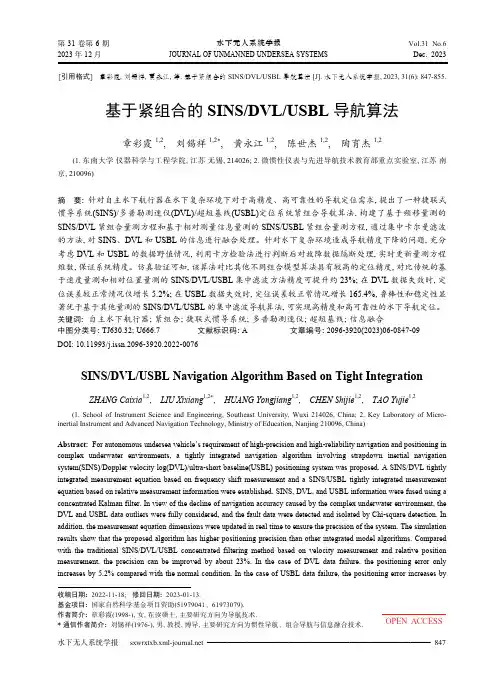
基于紧组合的SINS/DVL/USBL导航算法章彩霞 1,2, 刘锡祥 1,2*, 黄永江 1,2, 陈世杰 1,2, 陶育杰 1,2(1. 东南大学 仪器科学与工程学院, 江苏 无锡, 214026; 2. 微惯性仪表与先进导航技术教育部重点实验室, 江苏 南京, 210096)摘 要: 针对自主水下航行器在水下复杂环境下对于高精度、高可靠性的导航定位需求, 提出了一种捷联式惯导系统(SINS)/多普勒测速仪(DVL)/超短基线(USBL)定位系统紧组合导航算法, 构建了基于频移量测的SINS/DVL紧组合量测方程和基于相对测量信息量测的SINS/USBL紧组合量测方程, 通过集中卡尔曼滤波的方法, 对SINS、DVL和USBL的信息进行融合处理。

针对水下复杂环境造成导航精度下降的问题, 充分考虑DVL和USBL的数据野值情况, 利用卡方检验法进行判断后对故障数据隔断处理, 实时更新量测方程维数, 保证系统精度。

仿真验证可知, 该算法对比其他不同组合模型算法具有较高的定位精度, 对比传统的基于速度量测和相对位置量测的SINS/DVL/USBL集中滤波方法精度可提升约23%; 在DVL数据失效时, 定位误差较正常情况仅增长5.2%; 在USBL数据失效时, 定位误差较正常情况增长165.4%, 鲁棒性和稳定性显著优于基于其他量测的SINS/DVL/USBL的集中滤波导航算法, 可实现高精度和高可靠性的水下导航定位。

关键词: 自主水下航行器; 紧组合; 捷联式惯导系统; 多普勒测速仪; 超短基线; 信息融合中图分类号: TJ630.32; U666.7 文献标识码: A 文章编号: 2096-3920(2023)06-0847-09DOI: 10.11993/j.issn.2096-3920.2022-0076SINS/DVL/USBL Navigation Algorithm Based on Tight IntegrationZHANG Caixia1,2,　LIU Xixiang1,2*,　HUANG Yongjiang1,2,　CHEN Shijie1,2,　TAO Yujie1,2(1. School of Instrument Science and Engineering, Southeast University, Wuxi 214026, China; 2. Key Laboratory of Micro-inertial Instrument and Advanced Navigation Technology, Ministry of Education, Nanjing 210096, China)Abstract: For autonomous undersea vehicle’s requirement of high-precision and high-reliability navigation and positioning in complex underwater environments, a tightly integrated navigation algorithm involving strapdown inertial navigation system(SINS)/Doppler velocity log(DVL)/ultra-short baseline(USBL) positioning system was proposed. A SINS/DVL tightly integrated measurement equation based on frequency shift measurement and a SINS/USBL tightly integrated measurement equation based on relative measurement information were established. SINS, DVL, and USBL information were fused using a concentrated Kalman filter. In view of the decline of navigation accuracy caused by the complex underwater environment, the DVL and USBL data outliers were fully considered, and the fault data were detected and isolated by Chi-square detection. In addition, the measurement equation dimensions were updated in real time to ensure the precision of the system. The simulation results show that the proposed algorithm has higher positioning precision than other integrated model algorithms. Compared with the traditional SINS/DVL/USBL concentrated filtering method based on velocity measurement and relative position measurement, the precision can be improved by about 23%. In the case of DVL data failure, the positioning error only increases by 5.2% compared with the normal condition. In the case of USBL data failure, the positioning error increases by收稿日期: 2022-11-18; 修回日期: 2023-01-13.基金项目: 国家自然科学基金项目资助(51979041、61973079).作者简介: 章彩霞(1998-), 女, 在读硕士, 主要研究方向为导航技术.* 通信作者简介: 刘锡祥(1976-), 男, 教授, 博导, 主要研究方向为惯性导航、组合导航与信息融合技术.第 31 卷第 6 期水下无人系统学报Vol.31 N o.6 2023 年 12 月JOURNAL OF UNMANNED UNDERSEA SYSTEMS Dec. 2023[引用格式] 章彩霞, 刘锡祥, 黄永江, 等. 基于紧组合的SINS/DVL/USBL导航算法[J]. 水下无人系统学报, 2023, 31(6): 847-855.165.4% compared with the normal condition, and the robustness and stability are significantly better than the SINS/DVL/USBL concentrated filtering navigation algorithm based on other measurements. Therefore, it can achieve high-precision and high-reliability underwater navigation and positioning.Keywords: autonomous undersea vehicle; tight integration; strapdown inertial navigation system; Doppler velocity log; ultra-short baseline; information fusion0　引言准确的定位和导航信息是自主水下航行器(autonomous undersea vehicle, AUV)安全、高效作业的关键[1-2]。

飞向天空的小汽车英语作文300字In the realm of technological advancements, where the boundaries of human ingenuity are constantly pushed, a futuristic marvel emerged—the skybound automobile. This extraordinary invention ignited the imaginations of countless individuals, promising to revolutionize transportation and redefine the concept of mobility.Envision a sleek, aerodynamic vehicle, its body glistening with a metallic sheen. Equipped with advanced propulsion systems, this automobile possesses the ability to defy gravity and soar through the skies. Its wings, meticulously engineered to maximize lift and maneuverability, unfurl gracefully as it prepares for takeoff.As the engines hum to life, a surge of excitement courses through the veins of the occupants. With a gentle ascent, the skybound automobile rises from the ground, leaving behind the mundane constraints of terrestrialtravel. The cityscape below transforms into a miniature landscape, as the vehicle ascends towards the vast expanseof the sky.Piloting this aerial marvel is an experience unlike any other. The controls respond with precision, allowing for effortless navigation through the three-dimensional realm. The city's skyline stretches out before your eyes, offering a breathtaking panoramic view. Buildings, once toweringover the streets, now appear as mere specks in the distance.The skybound automobile is not merely a means of transportation; it is a symbol of freedom and boundless possibilities. It liberates individuals from thelimitations of road traffic and enables them to traverse distances in a fraction of the time. Whether it's a quick commute to work or an impromptu adventure, this futuristic vehicle empowers people to reach their destinations swiftly and effortlessly.Furthermore, the skybound automobile boastsunparalleled environmental credentials. Its advancedpropulsion systems eliminate harmful emissions,contributing to a cleaner and more sustainable future. By reducing the reliance on fossil fuels, this innovative invention plays a vital role in mitigating climate change and preserving the planet's well-being.As the skybound automobile continues to evolve, its capabilities will undoubtedly expand. Imagine vehicles equipped with autonomous navigation systems, allowing for hands-free flight. Or perhaps, personal air taxis that provide a convenient and affordable mode of aerial transportation. The possibilities are endless.The advent of the skybound automobile marks a pivotal moment in human history. It is a testament to the ingenuity and determination of engineers and innovators who dared to dream of a world where the skies are no longer a distant aspiration, but an accessible realm of exploration and limitless potential.。

基于iGMAS的BDS空间信号精度性能评估张璞;陈国通;张晓旭;邵士凯;郝菁;王小娜【摘要】全球连续监测评估系统(international GNSS Monitoring&Assessment System,iGMAS)是我国为了向导航用户提供安全可靠的全球卫星导航系统(Global Navigation Satellite System,GNSS)服务而搭建的对导航性能指标进行监测和评估的平台.在卫星导航系统中,空间信号精度的优劣直接决定卫星导航的定位精度,因此对空间信号精度的评估十分必要.此次研究基于iGMAS提供的广播星历和精密星历产品,通过分段法求得用户测距误差,然后使用差分法分别求得用户测速误差和用户加速度误差.实验结果表明,用户测距误差、用户测速误差、用户加速度误差均达到国际精度(95％置信度),iGMAS下的广播星历数据可作为评估空间信号的数据来源;我国的iGMAS已经较为成熟,可作为评估空间信号精度的平台.【期刊名称】《通信技术》【年(卷),期】2018(051)008【总页数】8页(P1820-1827)【关键词】全球连续监测评估系统;用户测距误差;用户测速误差;用户加速度误差;广播星历;精密星历【作者】张璞;陈国通;张晓旭;邵士凯;郝菁;王小娜【作者单位】河北科技大学,河北石家庄 050018;卫星导航与装备技术国家重点实验室,河北石家庄 050000;河北科技大学,河北石家庄 050018;河北科技大学,河北石家庄 050018;卫星导航与装备技术国家重点实验室,河北石家庄 050000;河北科技大学,河北石家庄 050018;卫星导航与装备技术国家重点实验室,河北石家庄050000;中国电子科技集团公司第五十四研究所,河北石家庄 050000;河北科技大学,河北石家庄 050018【正文语种】中文【中图分类】TP288.40 引言国际全球连续监测评估系统（international GNSS Monitoring & Assessment System，iGMAS）的基本功能是数据监测采集、传输、贮存、分析与信息发布，建设目的主要是为用户提供安全可靠的全球卫星导航系统（Global Navigation Satellite System，GNSS）服务[1]。

单目三维重建综述英文回答：Monocular 3D Reconstruction: A Comprehensive Review.Introduction.Monocular 3D reconstruction is the task of estimating the 3D structure of a scene from a single 2D image. This is a challenging problem, as the lack of multiple viewpoints makes it difficult to disambiguate depth and 3D relationships. However, monocular 3D reconstruction has a wide range of applications, including robotics, autonomous driving, and augmented reality.Methods.There are a variety of methods for monocular 3D reconstruction. These methods can be broadly divided into two categories:Geometric methods: These methods use geometric constraints to infer the 3D structure of a scene. For example, vanishing points can be used to estimate the location of the camera and the orientation of planes in the scene.Learning-based methods: These methods use machine learning techniques to learn the mapping from a single 2D image to a 3D representation. For example, convolutional neural networks (CNNs) can be trained to predict the depth map of a scene from a single image.Evaluation.The performance of monocular 3D reconstruction methods is typically evaluated using a variety of metrics, including:Accuracy: The accuracy of a method is measured by the mean absolute error (MAE) between the predicted 3Dstructure and the ground truth.Completeness: The completeness of a method is measured by the percentage of the ground truth 3D structure that is correctly predicted.Robustness: The robustness of a method is measured by its ability to handle challenging conditions, such as noise, occlusions, and motion blur.Applications.Monocular 3D reconstruction has a wide range of applications, including:Robotics: Monocular 3D reconstruction can be used to create maps of the environment for robots. This information can be used for planning, navigation, and object manipulation.Autonomous driving: Monocular 3D reconstruction can be used to create depth maps of the road ahead. Thisinformation can be used to detect obstacles, plan safepaths, and control the vehicle's speed.Augmented reality: Monocular 3D reconstruction can be used to create virtual objects that can be placed in the real world. This technology can be used for gaming, education, and training.Conclusion.Monocular 3D reconstruction is a challenging but important problem with a wide range of applications. In recent years, there has been significant progress in this area, thanks to the development of new methods and the availability of large datasets. As this field continues to develop, we can expect to see even more accurate, complete, and robust monocular 3D reconstruction methods.中文回答：单目三维重建，综述。

Mechatronics and Control Systems As a mechatronics and control systems expert, I am passionate about the intersection of mechanical engineering, electronics, computer science, and control theory. This field allows me to design and create innovative systems that can automate processes, improve efficiency, and enhance overall performance. Theability to blend different disciplines and technologies to solve complex problems excites me and drives my work in this area. One of the key aspects of mechatronics and control systems is the integration of sensors and actuators to gather data, process information, and make decisions in real-time. This enables me to develop intelligent systems that can adapt to changing conditions and optimize performance. Whether it's designing a robotic arm for precise manufacturing tasks or developing an autonomous vehicle for navigation, the ability to control and monitor these systems is crucial for their success. In addition to technical skills, mechatronics and control systems also require a deep understanding of mathematical modeling, system dynamics, and control algorithms. By utilizing mathematical tools such as differential equations, Laplace transforms, and state-space representations, I can analyze system behavior, design controllers, and predict system responses. This analytical approach allows me to fine-tune system parameters, optimize performance, and ensure stability in dynamic systems. Moreover, mechatronics and control systems play a vital role in various industries, including automotive, aerospace, robotics, and manufacturing. By applying my expertise in this field, I can contribute to the development of cutting-edge technologies, improve product quality, and enhance operational efficiency. Whether it's designing a control system for a drone to deliver medical supplies in remote areas or implementing automation solutions in a smart factory, the impact of mechatronics and control systems is far-reaching and transformative. Furthermore, the rapid advancements in technology, such as artificial intelligence, machine learning, and Internet of Things (IoT), are driving innovation in mechatronics and control systems. By leveraging these emerging technologies, I can develop more intelligent and adaptive systems that can learn from data, make informed decisions, and continuously improve performance. This constant evolution and innovation inthe field excite me and motivate me to stay updated with the latest trends anddevelopments. In conclusion, mechatronics and control systems offer a unique blend of creativity, technical expertise, and problem-solving skills that enable me to design and develop innovative solutions for a wide range of applications. By integrating mechanical, electrical, and computer engineering principles, I can create intelligent systems that can automate tasks, enhance productivity, and improve overall performance. The interdisciplinary nature of this field challenges me to think outside the box, push boundaries, and explore new possibilities. My passion for mechatronics and control systems drives me to continue learning, experimenting, and innovating to make a positive impact on society and contribute to the advancement of technology.。

外文原文：RobotG. Gary WangAssistantProfessorDept.ofMechanicalandIndustrialEngineering,UniversityofManitoba,Winni peg,MB, R3T 5V6 CanadaeRobot's classificationSeveral thousand years ago the humanity longed for that makes one kind of elephant person's same machine, in order to extricates the humanity from the arduous work. If the ancient Greece poet Homeros lengthy narrative poem "Yiliyate" god of lame sea time of Si Tesi smelting, uses the gold casting to have a beautiful intelligent maidservant; Greek mythology "Lu Elder brother Discovery ship" bronze giant Tailuosi (Taloas); Judea in fable's soil giant and so on, these beautiful myth times were driving the people must certainly become the beautiful myth the reality, as early as started before two millenniums to present the automatic wooden figurine and some simple mechanical figurines. to the modern times, in after a robot word's appearance and the world the first industry robot comes out, the different function's robot also one after another appears, and enlivened in the different domain, from the space to the underground, developed from the industry broadly to the agriculture, the forest, the herd, the fishing, even entered the common family. Robot's many type, broad application, affects the depth, is we are unexpected. Divides from robot's use, may divide into two broad headings:Military robot:◆ ground military robotThe ground robot is mainly refers to the intelligence or the remote control wheeled and the track-laying vehicle. The ground military robot may divide into the independent vehicles and half independent vehicles. The independent vehicles depend upon the own intelligent autonomous navigation, the avoidance obstacle,the independence complete each kind of combat mission; Half independent vehicles may exercise independently under person's surveillance, when encounters the difficulty the operators may carry on the remote control intervention.◆ unmanned aerial vehicleIs called the airborne robot's unmanned aerial vehicle is in the military robot develops the quickest family, the first autopilot has been published since 1913, unmanned aerial vehicle's fundamental type has achieved 300 many kinds, at present the unmanned aerial vehicle which sells in the world market has 40 many kinds. The US participated in nearly the world all important wars. Is advanced as a result of its science and technology, the national strength is strong, thus 80 for many years, the world unmanned aerial vehicle's development basically has been prompts forward by the line. The US studies one of unmanned aerial vehicle earliest countries, regardless of today looking from technical level or unmanned aerial vehicle's type and quantity, the US occupies the world leader. the comprehensive survey unmanned aerial vehicle develops the history, may say that the modern warfare is the power which the unmanned aerial vehicle develops, the high technology and new technology development is the foundation which it progresses unceasingly.◆ underwater robotThe underwater robot divides into some person of robots and nobody robot two broad headings:Some person of submersibles mobile nimble, is advantageous for the processing complex question, holds the post the life will possibly have the danger, moreover the price will be expensive. The unmanned submersible is the underwater robot which the people said that “Shinao” is one kind. It is suitable for the long time, the wide range inspection duty, in the recent 20 years, the underwater robot had the very big development, they both may military and be possible civil.Further develops along with the human to the sea, in the 21st century they will certainly to have a more widespread application. According to the unmanned submersible and the water surface support equipment (depot ship or platform) contact method's difference, the underwater robot may divide into two broad headings: One kind has the cable underwater robot, in the custom is called as it controls remotely the submersibles, is called ROV; Another kind does not have the cable underwater robot, in the submersibles custom is called as it the autonomous submersibles, is called AUV. Has the cable robot is the remote control type, divides into towed, (seabed) according to its mode of motion the mobile and the float (from navigation) the formula three kinds. Does not have the cable underwater robot only to be able to be autonomous -like, at present also only then the observation float type one mode of motion, but its prospect is bright.◆ spatial robotThe spatial robot is one kind of low end light teleoperator, may in the planet atmospheric environment the guidance and the flight. Therefore, it must overcome many difficulties, for example it must be able, in changes unceasingly in three dimensional environment movement and autonomous navigation; Cannot pause nearly; Must be able real-time to determine it in the spatial position and the condition; Must be able to carry on the control primarily to the American its vertical movement; Must forecast and plan the way for its star border flight.Civil robot:◆ industry robotThe industry robot is refers to the industry the application one kind can carry on the automatic control, to be possible to duplicate programs, multi-purpose, the multi-degrees-of-freedom, the multipurpose operation machine, can transport the material, the work piece or manages the tool, withcompletes each kind of work. And this kind of operation machine may fix in a place, may also on the reciprocal motion car.◆ service robotThe service robot is in a robot family's young member, so far still did not have a strict definition, the different country to serves robot's understanding also to have certain difference. Serves robot's application scope to be very broad, is mainly engaged in work and so on maintenance, maintenance, repair, transportation, clean, security, rescue, guardianship. The German production technology and Institute of Automation manager executed Dr. Lafute for to serve the robot to give this kind of definition: Serves the robot is the shifter which one kind may program freely, it should have three motive axles at least, may partially or the completely automatic completes the services. Here services refer to are not the servicing activities which is engaged in for the industrial production goods, but refers to the services which the manner and the unit complete.◆ entertainment robotThe entertainment robot take watches, the entertainment for the human as a goal, has robot's exterior characteristic, may look like the human, some kind of animal, looks like in the fairy tale or the science fiction character likely and so on. Simultaneously has robot's function, may walk or complete the movement, may have the verbal skill, will sing, has certain sensation ability.◆ kind of person robotMay see from other category's robot, the majority robots do not look like the human, some do not even have a person's appearance, this point to cause many robot amateurs to be greatly disappointed. Perhaps you will ask, for system class person robot? Such robot will be easier to let the human accept. Actually,develops the outward appearance and the function and person's same robot is the desire which the scientists long for even in dreams, is also the goal which they pursue unremittingly. However, develops the performance outstanding kind of person robot, its biggest difficulty is both feet erectness walks. Because the robot and person's study way is dissimilar. A baby wants to study first walks, then studies runs; But the robot must study first runs, then studies walks. That is the robot study runs easier.◆ agricultural robotBecause the mechanization, the automaticity are quite backward, “the surface faces upwards toward the loess back, did not have time throughout the year” has become our country farmer's symbol. But recent years agricultural robot's being published, hopefully changed traditional the work way. In the agricultural robot's aspect, Japan resides in head at present the various countries.Robot historyUSThe US is robot's birthplace, as early as developed in the world in 1962 the first industry robot, compares was known as " the robot kingdom " Japan to start must at least early 56 years. After more than 30 years development, the US already became one in world robot powerful nations, the foundation is abundant, technological advance. The comprehensive survey its history, the path is winding, is not smooth.Because The US government from the 60s to the 70s's in ten several years period, has not included the industry robot the prioritize project, was only has done some research work in several universities and the minority company. Regarding the enterprise, in only saw the momentary interests of the day, the government does not have the financial support in the situation, rather misses the good opportunity, defends stubbornly in the use rigidity automation installment, isalso not willing to run risks, applies or makes the robot. In addition, at that time the American unemployment rate reached as high as 6.65%, the government worried that the development robot can cause more people to be unemployed, therefore does not give the investment, also does not organize to develop the robot, this has no alternative but saying that is The US government's strategic decision is wrong. In the late 70s, although The US government and the business community had take seriously, but still placed in the technical route the key point the research robot software and the military, the universe, the sea, the nuclear engineering and so on the special domain high-quality robot's development, caused Japan's industry robot to catch up, and surpassed the US very quickly in industrial production's application and the robot manufacturing industry, the product has formed the strong competitive power in the international market.After the 80s, the US only then feels the situation to be urgent, the government and the business community only then truly takes seriously to the robot, in the policy also has manifests, on the one hand encourages the industrial world development and the application robot, on the other hand the making plan, the enhancement investment, increase robot's research funds, regards as the American once more industrialization the robot the characteristic, causes US's robot rapidly expand.In the late 80s, applies robot's technical gradually maturing along with each big factory, the first generation of robot's technical performance could be getting more and more dissatisfied the actual need, the US starts to produce has the second generation of robot which the vision, the strength thought that and has seized the American 60% robot market very quickly. the US passes through one in the robot history to take the fundamental research freely, the neglect application development research road diversion, but US's robot technology internationally still has been in the leading position. Its technology is comprehensive, is advanced, the compatibility is also very strong. Concrete manifestation in:(1) the perform reliably, the function is comprehensive, the precision is high;(2) the robot language study development is quick, the linguistic type many, applies broadly, the level comes first in of high world;(3) the intelligence technological development is quick, its vision, sense of touch and so on artificial intelligence technology already in astronautics, automobile industry widespread application;(4) high development and so on intelligent, high difficulty military robot, outer space robot are rapid, mainly uses in the mine clearance, laying mines, the reconnaissance, to stand guard and the outer space survey aspect.EnglandAs early as in 1966, American Unimation Corporation's You Ni the Munder robot and the AMF Corporation's fertile sha especially blue robot already took the lead to enter the British market. in 1967 Britain's two greatly mechanical companies also especially for American these two robot company in British sales promotion robot. Then, British Hall Automation Corporation develops own robot RAMP. In the early 70s, because the British government Scientific research Committee has promulgated the denial artificial intelligence and robot's Lighthall reported that has implemented the limit development stern measures to the industry robot, thus the robot industry is unable to recover, almost resides in the lowliest place in Western Europe.But, internationally the robot vigorous development's situation very quickly causes the British Government to realize: Robot technology's backwardness, causes its commodity in international market competitive power is the drop greatly. Therefore, started from the late 70s, the British government transferred has the support manner, carried out and implements has a series of supported the policies and measures which the robot developed, like the widespread propaganda used robot's importance, in the finance for the purchase robot enterprise subsidy, to promote the robot research unit and the cartelpositively and so on, made the British robot to start the prosperous time which and developed vigorously in the realm of production widespread application.FranceFrance not only resides in the world leader in the robot capacity, moreover is in the world advanced level in the robot application level and the application scope. This mainly gives credit the French government quite takes the robot technology from the very beginning, specially places the key point develops in robot's applied research.The French robot's development is quite smooth, the primary cause is the research project which supports vigorously through the government, establishes a complete science and technology system. Namely by Official organization some robot foundation technology aspect research project, but applies and develops the aspect by the industrial world support development the work, both complement one another, cause the robot at the French business community very quick development and the popularization.GermanThe Germany industry robot's total occupies world third, is only inferior to Japan and the US. Here said Germany, what mainly refers to is original Federal Republic of Germany. It compared to British and Sweden introduction robot approximately late 56 years. Its therefore so, is because of a Germany's robot industry start, met the domestic economy not to be booming. But Germany's social environment is actually is advantageous to the robot industrial development. Because of the war, causes the labor force to be short, as well as the national technical level is high, is realizes uses robot's advantage. To the 70s mid and late part, the government has used the administrative method to pave the way for robot's promotion; Stipulated in " the improvement work condition plan " that has the danger regarding some, virulently, the harmful operating post, mustreplace average person's work by the robot. This plan has developed the widespread market for robot's application, and promoted the industry robot technology development. The Rierman nationality is any scientist does not grind the heavy actual nationality, they always insisted the technical application and the social demand unify principle. Is likely same besides the majority countries, the robot main application in the automobile industry, a prominent spot is Germany in the textile industry with the modernized production technological transformations original enterprise, has discarded the old machine, has purchased the modernized automatic equipment, the electronic accounting machine and the robot, causes the textile industry cost to drop, the quality to enhance, the product color and pattern varieties even more is suitable for sale. Caused to 1984 the profession which explained is " is on one's last legs " to promote finally. Meanwhile, Germany saw the robot and so on advanced automated technology to industrial production's function, proposed after 1985, the goal which must to high-level, the belt feel the intelligence robot which shifts. After near ten year endeavors, its intelligent robot's research and the application aspect are in the recognition in the world the leading position.RussianIn the former Soviet Union (is mainly in Russia), discusses the robot technology from the theory and the practice is from 50 niandai houbanqi starts. Started the robot prototype's research work to the late 50s. in 1968 trial produced a deep water work robot successfully. in 1971 developed the multi-purpose robots which the factory used. As early as (in 1970 11,975 years) started when the former Soviet Union ninth five-year plan, developed the robot to include in the country scientific technological advance guiding principle. To 1975, has developed 30 models 120 robots, passes through 20 year endeavor, former Soviet Union's robot in quantity, the quality water on is at the world leader position. The country has the destination to enhance the science and technology progress to treat as the impetus social product development the method,arranges robot's research manufacture; The related robot's research production, applies, the promotion and the enhancement work, arranges by the government, to have the plan, to carry on according to the step.ChinaSome people believed that is only to save the labor force using the robot, but our country pool of labor power is rich, develops the robot not necessarily to tally with our country national condition. This is one kind of misunderstanding. In our country, socialist system's superiority had decided the robot can display its strong point fully. It not can only bring the high productive forces and the huge economic efficiency for our country's economic development, moreover for our country's universe development, the ocean development, the nuclear power using and so on emerging domain's development will make the remarkable contribution。

我发明了无人飞机350字作文英文回答：The Invention of My Drone.As an innovator with a passion for technology, I present my latest creation: a cutting-edge drone that pushes the boundaries of aerial exploration. This unmanned aerial vehicle (UAV) is the culmination of meticulous design, advanced engineering, and a deep understanding of aerodynamics.Unveiling the Drone's Capabilities.My drone boasts an exceptional payload capacity, enabling it to carry specialized equipment for various applications. Its long-range capabilities and extended flight time allow for comprehensive aerial coverage and extended mission durations. Advanced sensors, including cameras and thermal imaging, provide real-time datacollection and situational awareness.Precision Control and Navigation.The drone's intuitive control system offers seamless flight management. Its advanced autopilot ensures stability and precision, while the obstacle avoidance algorithm empowers safe and efficient navigation. GPS-based positioning and autonomous flight modes enhance mission planning and execution.Versatility and Applications.The drone's versatility extends to a wide spectrum of industries and applications. In agriculture, it can monitor crop health, facilitate precision farming, and improveyield optimization. In construction, it offers aerial inspections, progress monitoring, and safety assessments. In search and rescue operations, it provides real-time situational awareness, enhances search efficiency, and assists in disaster response.Conclusion.My drone stands as a testament to human ingenuity and the boundless possibilities of technological advancement. It empowers users with an unparalleled level of aerial control, data collection, and situational awareness. As the frontiers of aerial exploration continue to expand, my drone will serve as an indispensable tool for innovation, efficiency, and progress.中文回答：无人机发明。

为人类带来便捷英语作文Title: The Impact of Technology on Human Convenience。

Technology has revolutionized the way we live, providing unparalleled convenience and efficiency in various aspects of our lives. From communication to transportation, from healthcare to education, technology has become an indispensable part of the human experience, significantly enhancing convenience for individuals worldwide.One of the most noticeable areas where technology has brought convenience is communication. The advent of smartphones, social media platforms, and instant messaging apps has made it easier than ever to connect with people across the globe. Whether it's keeping in touch with loved ones, collaborating with colleagues, or networking with professionals, communication technology has broken down barriers and facilitated seamless interaction irrespective of geographical distances.Moreover, the rise of e-commerce platforms has transformed the way we shop. With just a few clicks or taps, consumers can browse through a vast array of products, compare prices, read reviews, and make purchases without ever leaving the comfort of their homes. This convenience has not only saved time and effort but has also opened up access to a broader range of goods and services, including those not available locally.In the realm of transportation, technological advancements have revolutionized the way we travel. Ride-hailing services have made getting from one place toanother more convenient than ever, allowing users to summon a vehicle with the touch of a button. Additionally, navigation apps provide real-time traffic updates and alternate routes, helping individuals navigate congested roads more efficiently. Furthermore, the emergence ofelectric and autonomous vehicles holds the promise of safer, cleaner, and more convenient transportation in the future.Healthcare is another area where technology has had aprofound impact on convenience. Telemedicine services enable patients to consult with healthcare professionals remotely, eliminating the need for travel and reducing waiting times. Moreover, wearable health monitoring devices allow individuals to track their vital signs and activity levels continuously, empowering them to take proactive steps towards better health. Additionally, electronic health records ensure that patient information is easily accessible to healthcare providers, streamlining the delivery of care.In the field of education, technology hasrevolutionized learning and made it more accessible than ever before. Online courses and educational platforms offer flexible learning options, allowing individuals to acquire new skills and knowledge at their own pace and convenience. Virtual classrooms and digital learning tools provide interactive and engaging learning experiences, transcending the limitations of traditional brick-and-mortar education.Furthermore, technology has revolutionized the way we manage our daily tasks and responsibilities. From smarthome devices that automate household chores to productivity apps that help us organize our schedules and streamline workflows, technology has become an indispensable tool for enhancing efficiency and convenience in our everyday lives.However, it is essential to acknowledge that the convenience offered by technology comes with its own set of challenges and considerations. Issues such as privacy concerns, digital divide, and technological dependency need to be addressed to ensure that the benefits of technology are accessible to all and do not exacerbate existing inequalities.In conclusion, technology has brought unparalleled convenience to the lives of individuals worldwide, transforming how we communicate, shop, travel, receive healthcare, learn, and manage our daily tasks. By harnessing the power of technology responsibly and addressing its challenges, we can continue to enhance human convenience and improve the quality of life for people everywhere.。

神舟宇宙飞船英语作文Title: The Shenzhou Spacecraft: A Triumph of Chinese Space Exploration。

China's Shenzhou spacecraft represents a pinnacle in the nation's space exploration endeavors. With its groundbreaking missions and technological advancements, the Shenzhou program has propelled China into the ranks of leading spacefaring nations. Let's delve into the intricacies of this remarkable spacecraft and its significance in the realm of space exploration.Origins and Development。

The Shenzhou spacecraft, developed by the China National Space Administration (CNSA), emerged from China's ambitious space exploration initiatives in the late 20th century. Its development was propelled by a combination of indigenous technological innovation and international collaboration. Drawing inspiration from previous Soviet andAmerican spacecraft designs, China embarked on a journey to create its own crewed space vehicle capable of carrying astronauts into orbit and beyond.Key Components and Capabilities。