Dybvig. An infrastructure for profile-driven dynamic recompilation
- 格式:pdf
- 大小:285.76 KB
- 文档页数:18

Shot cut一hypermesh网格划分⑴单元体的划分1.1梁单元该怎么划分?Replace可以进行单元结点合并,对于一些无法抽取中面的几何体,可以采用surface offset 得到近似的中面线条抽中线:Geom中的lines下选择offset,依次点lines点要选线段,依次选中两条线,然后Creat.建立梁单元:1进入hypermesh-1D-HyperBeam,选择standard seaction。
在standard section library 下选HYPER BEAM在standard section type下选择solid circle(或者选择其它你需要的梁截面)。
然后create。
在弹出的界面上,选择你要修改的参数,然后关掉并保存。
然后return.2 新建property,然后create(或者选择要更新的prop),名称为beam,在card image 中选择PBAR,然后选择material,然后create.再return.3 将你需要划分的component设为Make Current,在1D-line mesh,选择要mesh的lines,选择element size,选择为segment is whole line,在element config:中选择bar2,property 选择beam(上步所建的property).然后选择mesh。
现在可以欣赏你的beam单元了,用类似方法可以建立其他梁单元,据说bar单元可以承受轴向,弯曲的力,rod的只能承受拉压的力,beam可以承受各方向的力。
1.2 2D面单元的划分:利用2D- automesh划分网格(快捷键F12),所有2D都可以用这个进行划分网格。
(目前我只会用size and bias panel)1.3 3D四面体的划分:利用3D-tetramesh划分四面体网格,一般做普通的网格划分这个就够用了。

ctk plugin framework 编译-回复ctk plugin framework 编译是一个涉及软件开发和构建的过程。
对于任何软件开发者来说,编译是将源代码转换为可执行文件或库的关键步骤之一。
在本文中,我将一步一步地回答关于ctk plugin framework 编译的问题,以帮助读者更好地理解和使用该框架。
首先,让我们了解一下ctk plugin framework 是什么。
ctk plugin framework 是一个基于OSGi(开放服务网关联盟)规范的插件框架,它提供了一种动态加载和管理插件的机制。
通过使用ctk plugin framework,开发者可以将应用程序拆分为多个模块化的插件,并在运行时进行动态组合和加载。
这样,可以实现更灵活、可扩展和易于维护的应用程序架构。
现在,让我们来了解如何进行ctk plugin framework 的编译。
在编译ctk plugin framework 之前,我们需要准备以下工具和环境:1. 开发环境:确保您的计算机上安装了所需的开发环境,例如C++ 编译器、cmake、make 和pkg-config。
这些工具将帮助您构建ctk plugin framework。
2. 下载ctk plugin framework 源代码:您可以从ctk plugin framework 官方网站或代码仓库下载最新版本的源代码。
解压缩下载的源代码压缩包到您选择的目录中。
3. 创建构建目录:在源代码的根目录中,创建一个名为"build" 的目录。
这将是我们构建ctk plugin framework 的目录。
一旦准备就绪,我们可以开始编译ctk plugin framework。
按照以下步骤进行操作:步骤1:打开终端或命令提示符,并导航到ctk plugin framework 源代码根目录下。
步骤2:在终端中,输入以下命令以创建构建目录并导航到该目录:mkdir buildcd build步骤3:运行cmake 命令以生成构建脚本。
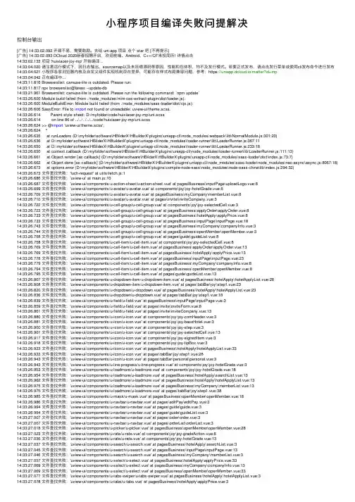
⼩程序项⽬编译失败问提解决控制台输出[⼴告] 14:33:02.092 开源不易,需要⿎励。
去给 uni-app 项⽬点个 star 吧 [不再提⽰][⼴告] 14:33:02.093 DCloud 2020新春招聘开启,欢迎前端、Android、C++/QT来投简历! 详情点击14:33:02.133 项⽬ 'huixiaoer-joy-mp' 开始编译...14:33:04.020 请注意运⾏模式下,因⽇志输出、sourcemap以及未压缩源码等原因,性能和包体积,均不及发⾏模式。
若要正式发布,请点击发⾏菜单或使⽤cli发布命令进⾏发布14:33:04.021 ⼩程序各家浏览器内核及⾃定义组件实现机制存在差异,可能存在样式布局兼容问题,参考:https://uniapp.dcloud.io/matter?id=mp14:33:04.042 正在编译中...14:33:11.816 Browserslist: caniuse-lite is outdated. Please run:14:33:11.817 npx browserslist@latest --update-db14:33:21.961 Browserslist: caniuse-lite is outdated. Please run the following command: `npm update`14:33:26.600 Module build failed (from ./node_modules/mini-css-extract-plugin/dist/loader.js):14:33:26.600 ModuleBuildError: Module build failed (from ./node_modules/sass-loader/dist/cjs.js):14:33:26.606 SassError: File to import not found or unreadable: uview-ui/theme.scss.14:33:26.614 Parent style sheet: D:/myfolder/code/huixiaoer-joy-mp/uni.scss14:33:26.614 on line 86 of ../../../../../code/huixiaoer-joy-mp/uni.scss14:33:26.624 >> @import 'uview-ui/theme.scss';14:33:26.624 ^14:33:26.635 at runLoaders (D:\myfolder\software\HBilderX\HBuilderX\plugins\uniapp-cli\node_modules\webpack\lib\NormalModule.js:301:20)14:33:26.636 at D:\myfolder\software\HBilderX\HBuilderX\plugins\uniapp-cli\node_modules\loader-runner\lib\LoaderRunner.js:367:1114:33:26.650 at D:\myfolder\software\HBilderX\HBuilderX\plugins\uniapp-cli\node_modules\loader-runner\lib\LoaderRunner.js:233:1814:33:26.650 at context.callback (D:\myfolder\software\HBilderX\HBuilderX\plugins\uniapp-cli\node_modules\loader-runner\lib\LoaderRunner.js:111:13)14:33:26.661 at Object.render [as callback] (D:\myfolder\software\HBilderX\HBuilderX\plugins\uniapp-cli\node_modules\sass-loader\dist\index.js:73:7)14:33:26.662 at Object.done [as callback] (D:\myfolder\software\HBilderX\HBuilderX\plugins\uniapp-cli\node_modules\sass-loader\node_modules\neo-async\async.js:8067:18) 14:33:26.673 at options.error (D:\myfolder\software\HBilderX\HBuilderX\plugins\compile-node-sass\node_modules\node-sass-china\lib\index.js:294:32)14:33:26.673 ⽂件查找失败:'luch-request' at utils\fetch.js:114:33:26.686 ⽂件查找失败:'uview-ui' at main.js:1014:33:26.687 ⽂件查找失败:'uview-ui/components/u-action-sheet/u-action-sheet.vue' at pagesBusiness\inputPage\uploadLogo.vue:814:33:26.699 ⽂件查找失败:'uview-ui/components/u-avatar/u-avatar.vue' at components\joy\joy-hotelGrade.vue:814:33:26.709 ⽂件查找失败:'uview-ui/components/u-avatar/u-avatar.vue' at pagesBusiness\myCompany\memberList.vue:814:33:26.710 ⽂件查找失败:'uview-ui/components/u-avatar/u-avatar.vue' at pages\invite\inviteCompany.vue:314:33:26.722 ⽂件查找失败:'uview-ui/components/u-cell-group/u-cell-group.vue' at components\joy\joy-selectedCell.vue:314:33:26.723 ⽂件查找失败:'uview-ui/components/u-cell-group/u-cell-group.vue' at pagesBusiness\applyOrder\applyOrder.vue:814:33:26.733 ⽂件查找失败:'uview-ui/components/u-cell-group/u-cell-group.vue' at pagesBusiness\hotelApply\applyPrice.vue:814:33:26.733 ⽂件查找失败:'uview-ui/components/u-cell-group/u-cell-group.vue' at pagesBusiness\inputPage\inputPage.vue:1814:33:26.743 ⽂件查找失败:'uview-ui/components/u-cell-group/u-cell-group.vue' at pagesBusiness\myCompany\companyInfo.vue:314:33:26.744 ⽂件查找失败:'uview-ui/components/u-cell-group/u-cell-group.vue' at pagesBusiness\openMember\openMember.vue:314:33:26.758 ⽂件查找失败:'uview-ui/components/u-cell-group/u-cell-group.vue' at pages\guide\guideList.vue:814:33:26.758 ⽂件查找失败:'uview-ui/components/u-cell-item/u-cell-item.vue' at components\joy\joy-selectedCell.vue:814:33:26.769 ⽂件查找失败:'uview-ui/components/u-cell-item/u-cell-item.vue' at pagesBusiness\applyOrder\applyOrder.vue:1314:33:26.769 ⽂件查找失败:'uview-ui/components/u-cell-item/u-cell-item.vue' at pagesBusiness\hotelApply\applyPrice.vue:1314:33:26.778 ⽂件查找失败:'uview-ui/components/u-cell-item/u-cell-item.vue' at pagesBusiness\inputPage\inputPage.vue:2314:33:26.779 ⽂件查找失败:'uview-ui/components/u-cell-item/u-cell-item.vue' at pagesBusiness\myCompany\companyInfo.vue:814:33:26.794 ⽂件查找失败:'uview-ui/components/u-cell-item/u-cell-item.vue' at pagesBusiness\openMember\openMember.vue:814:33:26.795 ⽂件查找失败:'uview-ui/components/u-cell-item/u-cell-item.vue' at pages\guide\guideList.vue:1314:33:26.807 ⽂件查找失败:'uview-ui/components/u-dropdown-item/u-dropdown-item.vue' at pagesBusiness\hotelApply\hotelApplyList.vue:2814:33:26.808 ⽂件查找失败:'uview-ui/components/u-dropdown-item/u-dropdown-item.vue' at pages\tabBar\joy\step1.vue:2314:33:26.820 ⽂件查找失败:'uview-ui/components/u-dropdown/u-dropdown.vue' at pagesBusiness\hotelApply\hotelApplyList.vue:2314:33:26.836 ⽂件查找失败:'uview-ui/components/u-dropdown/u-dropdown.vue' at pages\tabBar\joy\step1.vue:1814:33:26.839 ⽂件查找失败:'uview-ui/components/u-field/u-field.vue' at pagesBusiness\inputPage\inputPage.vue:314:33:26.859 ⽂件查找失败:'uview-ui/components/u-field/u-field.vue' at pages\invite\inviteForm.vue:814:33:26.861 ⽂件查找失败:'uview-ui/components/u-field/u-field.vue' at pages\invite\inviteCompany.vue:1314:33:26.880 ⽂件查找失败:'uview-ui/components/u-icon/u-icon.vue' at components\joy\joy-comHeader.vue:314:33:26.881 ⽂件查找失败:'uview-ui/components/u-icon/u-icon.vue' at components\joy\joy-baseHotel.vue:314:33:26.900 ⽂件查找失败:'uview-ui/components/u-icon/u-icon.vue' at components\joy\joy-step.vue:314:33:26.901 ⽂件查找失败:'uview-ui/components/u-icon/u-icon.vue' at components\joy\joy-selectedCell.vue:1314:33:26.917 ⽂件查找失败:'uview-ui/components/u-icon/u-icon.vue' at components\joy\joy-signedItem.vue:314:33:26.918 ⽂件查找失败:'uview-ui/components/u-icon/u-icon.vue' at components\joy\joy-tipBox.vue:314:33:26.933 ⽂件查找失败:'uview-ui/components/u-icon/u-icon.vue' at pagesBusiness\hotelApply\hotelApplyList.vue:3314:33:26.933 ⽂件查找失败:'uview-ui/components/u-icon/u-icon.vue' at pages\tabBar\joy\step1.vue:2814:33:26.943 ⽂件查找失败:'uview-ui/components/u-icon/u-icon.vue' at pages\tabBar\personal\personal.vue:314:33:26.943 ⽂件查找失败:'uview-ui/components/u-line-progress/u-line-progress.vue' at components\joy\joy-hotelGrade.vue:314:33:26.953 ⽂件查找失败:'uview-ui/components/u-loadmore/u-loadmore.vue' at components\joy\joy-hotelGrade.vue:1814:33:26.954 ⽂件查找失败:'uview-ui/components/u-loadmore/u-loadmore.vue' at pagesBusiness\hotelApply\searchList.vue:1314:33:26.962 ⽂件查找失败:'uview-ui/components/u-loadmore/u-loadmore.vue' at pagesBusiness\hotelApply\hotelApplyList.vue:1314:33:26.975 ⽂件查找失败:'uview-ui/components/u-loadmore/u-loadmore.vue' at pagesBusiness\myCompany\memberList.vue:1314:33:26.975 ⽂件查找失败:'uview-ui/components/u-loadmore/u-loadmore.vue' at pages\tabBar\joy\step1.vue:3814:33:26.985 ⽂件查找失败:'uview-ui/components/u-mask/u-mask.vue' at pagesBusiness\openMember\openMember.vue:1814:33:26.986 ⽂件查找失败:'uview-ui/components/u-navbar/u-navbar.vue' at pages\editPay\editPay.vue:314:33:26.994 ⽂件查找失败:'uview-ui/components/u-navbar/u-navbar.vue' at pages\guide\guide.vue:314:33:26.994 ⽂件查找失败:'uview-ui/components/u-navbar/u-navbar.vue' at pages\guide\guideList.vue:314:33:27.007 ⽂件查找失败:'uview-ui/components/u-navbar/u-navbar.vue' at pages\order\order.vue:314:33:27.007 ⽂件查找失败:'uview-ui/components/u-navbar/u-navbar.vue' at pages\orderList\orderList.vue:314:33:27.018 ⽂件查找失败:'uview-ui/components/u-picker/u-picker.vue' at pagesBusiness\openMember\openMember.vue:2814:33:27.023 ⽂件查找失败:'uview-ui/components/u-rate/u-rate.vue' at components\joy\joy-gradeAction.vue:814:33:27.036 ⽂件查找失败:'uview-ui/components/u-rate/u-rate.vue' at components\joy\joy-hotelGrade.vue:1314:33:27.037 ⽂件查找失败:'uview-ui/components/u-search/u-search.vue' at pagesBusiness\hotelApply\searchList.vue:314:33:27.045 ⽂件查找失败:'uview-ui/components/u-search/u-search.vue' at pagesBusiness\inputPage\inputPage.vue:1314:33:27.046 ⽂件查找失败:'uview-ui/components/u-search/u-search.vue' at pagesBusiness\myCompany\memberList.vue:314:33:27.057 ⽂件查找失败:'uview-ui/components/u-select/u-select.vue' at pagesBusiness\hotelApply\applyPrice.vue:3314:33:27.069 ⽂件查找失败:'uview-ui/components/u-select/u-select.vue' at pagesBusiness\myCompany\companyInfo.vue:1314:33:27.069 ⽂件查找失败:'uview-ui/components/u-select/u-select.vue' at pagesBusiness\openMember\openMember.vue:3314:33:27.077 ⽂件查找失败:'uview-ui/components/u-tabs-swiper/u-tabs-swiper.vue' at pagesBusiness\hotelApply\hotelApplyList.vue:314:33:27.078 ⽂件查找失败:'uview-ui/components/u-tabs/u-tabs.vue' at pagesBusiness\hotelApply\applyPrice.vue:314:33:27.091 ⽂件查找失败:'uview-ui/components/u-tabs/u-tabs.vue' at pages\tabBar\joy\step1.vue:8 14:33:27.092 ⽂件查找失败:'uview-ui/libs/function/md5' at utils\sign.js:114:33:27.103 ERROR Build failed with errors.解决⽅法:cmd进⼊项⽬跟⽬录,执⾏npm i 命令PS:npm命令找不到时需要先安装node.jsEND。
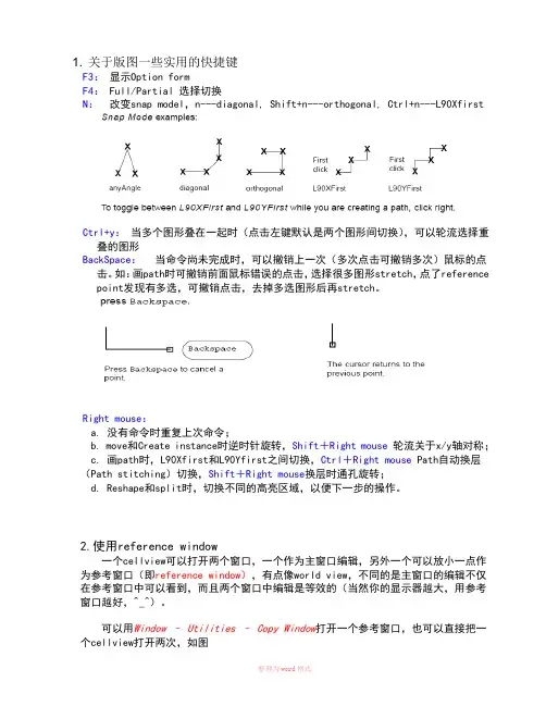
1. 关于版图一些实用的快捷键F3:显示Option formF4: Full/Partial 选择切换N:改变snap model,n---diagonal, Shift+n---orthogonal, Ctrl+n---L90XfirstCtrl+y:当多个图形叠在一起时(点击左键默认是两个图形间切换),可以轮流选择重叠的图形BackSpace:当命令尚未完成时,可以撤销上一次(多次点击可撤销多次)鼠标的点击。
如:画path时可撤销前面鼠标错误的点击,选择很多图形stretch,点了reference point发现有多选,可撤销点击,去掉多选图形后再stretch。
Right mouse:a. 没有命令时重复上次命令;b. move和Create instance时逆时针旋转,Shift+Right mouse轮流关于x/y轴对称;c. 画path时,L90Xfirst和L90Yfirst之间切换,Ctrl+Right mouse Path自动换层(Path stitching)切换,Shift+Right mouse换层时通孔旋转;d. Reshape和split时,切换不同的高亮区域,以便下一步的操作。
2.使用reference window一个cellview可以打开两个窗口,一个作为主窗口编辑,另外一个可以放小一点作为参考窗口(即reference window),有点像world view,不同的是主窗口的编辑不仅在参考窗口中可以看到,而且两个窗口中编辑是等效的(当然你的显示器越大,用参考窗口越好,^_^)。
可以用Window – Utilities – Copy Window打开一个参考窗口,也可以直接把一个cellview打开两次,如图可以同时在两个窗口中编辑3.关于Path stitching①画path时可以从一层切换到另一层,并且自动打上对应的接触孔,这个功能叫path stitching.②在Change To Layer 栏里选择你要换的layer,也可以通过Control+right mouse键来选择需要换的层。

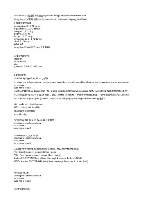
MiniGUI3.0.12及组件下载地址http://www.minigui.org/downloads/index.html libmgplus-1.2.4下载地址http://download.csdn.net/download/yong_f/4062807 1. 需要下载的组件 libminigui-gpl-3_0_12.tar.gz mg-samples-3_0_12.tar.gz freetype-1_3_1.tar.gz jpegsrc_v7.tar.gz libpng-1_2_37.tar.gz minigui-res-be-3_0_12.tar.gz zlib-1_2_2.tar.gz qvfb2-2.0
libmgplus-1.2.4(可以在csdn上下载到)
(qvfb所需要的包) libqt3-mt libqt3-mt-dev alien qt-devel-3.3.8-4.fc7.i386.rpm
2.安装各组件 <1>libminigui-gpl-3_0_12.tar.gz(库) ./configure --prefix=/usr/local –enable-procs --enable-videoqvfb --enable-qvfbial --disable-splash --disable-screensaver sudo make sudo make install
(gui默认安装的是gui-theads模式,加--enable-procs编译为MiniGUI-processes 模式。MiniGUI3.0.12版本默认情况下是不开QVFB图像引擎与QVFB输入引擎的,要加--enable-videoqvfb --enable-qvfbial配置项,不然会出现NEWGAL: Does not
find matched engine: qvfb.与InitGUI (step 4): Can not get graphics engine information!的情况)
![[Fluent] Solver error原因及处理方法综整](https://uimg.taocdn.com/3dda6e0ade80d4d8d15a4f96.webp)

对比React Native和Flutter的渲染性能React Native和Flutter是目前最受欢迎的跨平台移动应用开发框架,它们都具有高效的渲染性能,但在某些方面存在差异。
本文将对比React Native和Flutter的渲染性能,以帮助读者选择适合自己项目的框架。
一、React Native的渲染性能React Native是由Facebook推出的开源框架,基于JavaScript和React构建。
它使用了原生组件和视图系统来实现跨平台开发,具有一定的渲染性能优势。
1. JIT编译加速:React Native使用了Just-In-Time(JIT)编译技术,在运行时将JavaScript代码转换为本地机器代码,以提高性能。
这种编译方式可以显著加快应用的启动速度和页面渲染速度。
2. 增量更新:React Native通过Diffing算法实现了增量更新,只更新需要改变的部分,而不是整个页面进行重新渲染。
这种优化策略能够减少无效的渲染操作,提高渲染效率。
3. 异步渲染:React Native利用异步渲染机制,将UI渲染操作分解成多个小任务,并在渲染线程中异步执行。
这种方式可以避免UI线程的阻塞,提高应用的响应速度和流畅度。
二、Flutter的渲染性能Flutter是由Google开发的跨平台移动应用开发框架,使用Dart语言构建。
它采用了自绘引擎,并使用了Skia图形库进行界面渲染,具有独特的渲染性能优势。
1. 一切皆是Widget:Flutter的UI界面完全由Widget构成,包括布局、样式、交互等,保证了整个渲染过程的高效性和一致性。
Widget具有高性能和轻量级的特点,可以快速构建和渲染复杂的UI界面。
2. 优化的渲染管道:Flutter的渲染管道采用了基于GPU的渲染技术,避免了绘制繁重的中间层,减少了渲染过程中的性能损耗。
这种优化策略可以有效提高Flutter应用的渲染性能和响应速度。
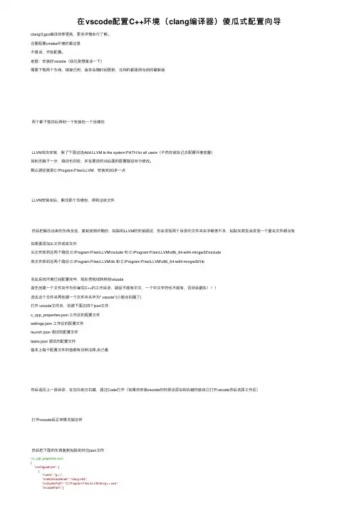
在vscode配置C++环境(clang编译器)傻⽠式配置向导clang⽐gcc编译效率更⾼,更多详情⾃⾏了解。
还要配置cmake环境的看这⾥不废话,开始配置。
前提:安装好vscode(我还是想废话⼀下)需要下载两个东西,链接已附,版本会随时间更新,这⽤的都是⽤当前的最新版两个都下载好后得到⼀个安装包⼀个压缩包LLVM双击安装,除了下图这选Add LLVM to the system PATH for all users(不然你就⾃⼰去配置环境变量)其他⽆脑下⼀步,路径也别改,实在要改的话后⾯的配置路径⾃⾏修改。
默认路径就是C:\Program Files\LLVM,安装完2G多⼀点LLVM安装完后,解压那个压缩包,得到这些⽂件然后把解压出来的东西全选,复制或剪切随你,粘贴到LLVM的安装路径,你会发现两个⽬录的⽂件夹名字都差不多,粘贴完甚⾄会发现⼀个重名⽂件都没有如果要添加头⽂件或库⽂件头⽂件放到这两个路径 C:\Program Files\LLVM\include 和 C:\Program Files\LLVM\x86_64-w64-mingw32\include库⽂件放到这两个路径 C:\Program Files\LLVM\lib 和 C:\Program Files\LLVM\x86_64-w64-mingw32\lib⾄此系统环境已经配置完毕,现在把视线转移到vscode⾸先创建⼀个⽂件夹作为你编写C++的⼯作⽬录,路径不能有中⽂,⼀个中⽂字符也不能有,否则会翻车进去这个⽂件夹再创建⼀个⽂件夹名字为".vscode"(⼩数点别漏了)打开.vscode⽂件夹,创建下⾯这四个json⽂件c_cpp_properties.json ⼯作区的配置⽂件settings.json ⼯作区的配置⽂件launch.json 调试的配置⽂件tasks.json 调试的配置⽂件基本上每个配置⽂件的值都有说明注释,⾃⼰看然后返回上⼀级⽬录,在空⽩地⽅右键,通过Code打开(如果你安装vscode的时候没添加到右键你就⾃⼰打开vscode然后选择⼯作区)打开vscode后正常情况就这样然后把下⾯的东西复制粘贴到对应json⽂件//c_cpp_properties.json{"configurations": [{"name": "g++","intelliSenseMode": "clang-x64","compilerPath": "C:/Program Files/LLVM/bin/g++.exe","${workspaceFolder}"],"defines": [],"browse": {"path": ["${workspaceFolder}"],"limitSymbolsToIncludedHeaders": true,"databaseFilename": ""},"cStandard": "c11","cppStandard": "c++17"}],"version": 4}// launch.json{// 使⽤ IntelliSense 了解相关属性。
C++Builder 资料库1.怎样在C++Builder中创建使用DLL2.用C++Bulider在WIN.INI中保存信息3.如何在C++Builder中检测硬件4.C++Builder如何响应消息及自定义消息5.利用C++ Builder开发动画DLL6.用C++ Builder 3制作屏幕保护程序7.TCP/IP头格式8.UDP9.判断windows的Desktop及其它目录10用C++Builder创建数字签名11用Enter 键控制焦点切换的方法12.拦截Windows 消息13.使用CommaText14.程序开始时先显示信息框15.怎样获取程序的命令行参数?16.如何监视剪贴板17.如何使用OnIdle事件18.用C++Builder编写串行异步通信程序19.C++BUILDER非可视组件的消息处理技巧20.用C++Builder 建立数据库VCL使用经验21.用C++ Builder创建基于Internet的点对点Chat22.用C++Builder获取应用程序图标23.BIG5到GB的转换技术24.C++BUILDER让你的任务栏图标动起来25.TFORM26.用BCB在windows桌面创建快捷方式27.读磁片磁区28.I/O 端口读写的实现29.检测鼠标位置30.令Win32 应用程序跳入系统零层31.如何取得Memo的行和列32.使用Sockets33.Windows95/98下怎样隐藏应用程序不让它出现在CTRL-ALT-DEL对话框中?34.怎样隐藏应用程序的任务条图标35.编写自己的Ping.exe程序36.用C++Builder在WINNT下编制一个Service37.如何在C++ BUILDER中自动关闭WINDOWS屏保38.显示/隐藏任务栏图标39.信箱监视程序40.C++Building制作闹钟41.拨号上网IP地址的检知42.用C++ Builder编写Tray程序43.怎样用代码来最小化或恢复程序44.制作主窗口显示前的版权窗口45.判断是否已经联到internet46.获取登陆用户名47.隐藏桌面图标48.程序启动时运行49.控制面板的调用50.模拟键盘按键51.让标题栏闪烁52.启动屏幕保护53.年月日星期的取法54.键盘事件55.隐藏任务栏56.禁止关机57.怎样以最小化方式启动程序58.在Memo中增加一行后,如何使最后一行能显示59.设置壁纸方法怎样在C++Builder中创建使用DLL自从C++Builder从去年浪漫情人节上市以来,吸引了大量的Delphi、VC、Vb的程序员到它的怀抱,大量的C、C++程序员感叹道:总算有了C的可视化开发工具,对我也是一样,从BC、Delphi到C++Builder。
关于surfer绘制等直线,由于需要结合自己实际需要绘制,sufer只能绘制2D等直线,所以首先确定自己绘制等直线的面,然后flac3d导出的单元信息(坐标及应力,应变),通过简单的fortran程序找出所要求的面上的单元的,并记录其坐标位置,即应力应变值。
输出格式为surfer认可的格式即可以了。
授人以鱼,不如授人以渔。
我编的程序只能针对自己的问题,所以大家不要关心程序,如果,确实需要,按照上述思路实现应该很容易。
建立模型以后直接solve让程序产生应力分布!虽然时间花费上多一点,可是不用那么伤脑筋了。
我得懒人做法是:1)现把模量×10,c,Fi取很大,然后solve for balance;2)ini disp=0,ini state =0,;3)回复原来得E,G,C,Fi等,subzone和zone哪个是“最小几何单位”?二者有和区别呢?我们通常说的“单元element”指的是哪一个?用户接触到的最小几何单位应该是zone通常说的element也是指zonesubzone和FLAC3d的Mixed Discretization算法有关比如说一个brick计算时又自动划分为2套overlay每套overlay中各有5个tetra即subzone据说这样可以更好地模拟材料的塑性变形这是flac3d为了避免求解中单元出现“沙漏”现象而采取的一种单元离散技术Q:gen zone brick size 6 6 6model elasprop bulk 1e8 shear 7e7fix x range x -0.1 0.1table 1 0,0 100,-1e5 /我不知道table在这里什么意思,有什么作用apply sxx 1.0 hist table 1 range x 5.9,6.1 y 0,6 z 0,2hist zone sxx 6,0,0step 100我对这个table不是很清楚gen zone cyl p0 0 0 0 p1 1 0 0 p2 0 2 0 p3 0 0 1 size 4 5 4gen zone reflect norm 1,0,0gen zone reflect norm 0,0,1model ssprop bulk 1.19e10 shear 1.1e10prop coh 2.72e5 fric 44 ten 2e5prop ttab 1table 1 0,2e5 2e-5,0请问这里的table和后面的数字到底是什么意思啊?A:table相当于数已经赋值的数组请问sel cable id=1 begin=(0.0, 0.5, 3.5) end=(8, 0.5, 3.5) nseg=8 中的nseg是什么意思?把cable分为几段,比如nseg=8 ,就是分为八段.gen zone reflect dip 90 dd 270 origin 0,0,0应该是以90 和270度还有原点组成的平面进行对称拷贝吧??ini state=0初始化单元为弹性。
在没有考虑vdw作用之前,算Bi2Se3材料soc中出现的错误汇总V ASP自旋轨道耦合计算错误汇总静态计算时,报错:VERY BAD NEWS! Internal内部error in subroutine子程序IBZKPT:Reciprocal倒数的lattice and k-lattice belong to different class of lattices. Often results are still useful (48)INCAR参数设置:对策:根据所用集群,修改INCAR中NPAR。
将NPAR=4变成NPAR=1,已解决!错误:sub space matrix类错误报错:静态和能带计算中出现警告:W ARNING: Sub-Space-Matrix is not hermitian共轭in DA V结构优化出现错误:WARNING: Sub-Space-Matrix is not hermitian in DA V 4 -4.681828688433112E-002对策:通过将默认AMIX=0.4,修改成AMIX=0.2(或0.3),问题得以解决。
以下是类似的错误:WARNING: Sub-Space-Matrix is not hermitian in rmm -3.00000000000000RMM: 22 -0.167633596124E+02 -0.57393E+00 -0.44312E-01 1326 0.221E+00BRMIX:very serious problems the old and the new charge density differ old charge density: 28.00003 new 28.06093 0.111E+00错误:WARNING: Sub-Space-Matrix is not hermitian in rmm -42.5000000000000ERROR FEXCP: supplied Exchange-correletion table is too small, maximal index : 4794错误:结构优化Bi2Te3时,log文件:WARNING in EDDIAG: sub space matrix is not hermitian 1 -0.199E+01RMM: 200 0.179366581305E+01 -0.10588E-01 -0.14220E+00 718 0.261E-01BRMIX: very serious problems the old and the new charge density differ old charge density: 56.00230 new 124.70394 66 F= 0.17936658E+01 E0= 0.18295246E+01 d E =0.557217E-02curvature: 0.00 expect dE= 0.000E+00 dE for cont linesearch 0.000E+00ZBRENT: fatal error in bracketingplease rerun with smaller EDIFF, or copy CONTCAR to POSCAR and continue但是,将CONTCAR拷贝成POSCAR,接着算静态没有报错,这样算出来的结果有问题吗?对策1:用这个CONTCAR拷贝成POSCAR重新做一次结构优化,看是否达到优化精度!对策2:用这个CONTCAR拷贝成POSCAR,并且修改EDIFF(目前参数EDIFF=1E-6),默认为10-4错误:WARNING: Sub-Space-Matrix is not hermitian in DA V 1 -7.626640664998020E-003网上参考解决方案:对策1:减小POTIM: IBRION=0,标准分子动力学模拟。
An Infrastructure for Profile-Driven Dynamic Recompilation∗Robert G.Burger R.Kent DybvigIndiana University Computer Science DepartmentLindley Hall215Bloomington,Indiana47405{burger,dyb}@September1997AbstractDynamic optimization of computer programs can dramatically improve their performance on avariety of applications.This paper presents an efficient infrastructure for dynamic recompilationthat can support a wide range of dynamic optimizations including profile-driven optimizations.The infrastructure allows any section of code to be optimized and regenerated on-the-fly,evencode for currently active procedures.The infrastructure incorporates a low-overhead edge-count profiling strategy that supportsfirst-class continuations and reinstrumentation of activeprocedures.Profiling instrumentation can be added and removed dynamically,and the datacan be displayed graphically in terms of the original source to provide useful feedback to theprogrammer.Keywords:edge-count profiling,dynamic compilation,run-time code generation,basic blockreordering1IntroductionIn the traditional model of program optimization and compilation,a program is optimized and compiled once,prior to execution.This allows the cost of program optimization and compilation to be amortized,possibly,over may program runs.On the other hand,it prevents the compiler from exploiting properties of the program,its input,and its execution environment that can be determined only at run time.Recent research has shown that dynamic compilation can dramatically improve the performance of a wide range of applications including network packet demultiplexing, sparse matrix computations,pattern matching,and mobile code[9,7,12,15,19,23].Dynamic optimization works when a program is staged in such a way that the cost of dynamic recompilation can be amortized over many runs of the optimized code[21].This paper presents an infrastructure for dynamic recompilation of computer programs that permits optimization of code at run time.The infrastructure allows any section of code to be∗This material is based on work supported in part by the National Science Foundation under grant numbers CDA-9312614and CCR-9711269.Robert G.Burger was supported in part by a National Science Foundation Graduate Research Fellowship.optimized and regenerated on-the-fly,even the code for currently active procedures.In our Scheme-based implementation of the infrastructure,the garbage collector is used tofind and relocate all references to recompiled procedures,including return addresses in the active portion of the control stack.Since many optimizations benefit from profiling information,we have included support for profiling as an integral part of the recompilation infrastructure.Instrumentation for profiling can be inserted or removed dynamically,again by regenerating code on-the-fly.A variant of Ball and Larus’s low-overhead edge-count profiling strategy[2],extended to supportfirst-class continuations and reinstrumentation of active procedures,is used to obtain accurate execution counts for all basic blocks in instrumented code.Although profiling overhead is fairly low,profiling is typically enabled only for a portion of a program run,allowing subsequent execution to benefit from optizations guided by the profiling information without the profiling overhead.A side benefit of the profiling support is that profile data can be made available to the program-mer,even as a program is executing.In our implementation,the programmer can view profile data graphically in terms of the original source(possibly split over manyfiles)to identify the“hot spots”in a program.The source is color-coded according to execution frequency,and the programmer can“zoom in”on portions of the program or portions of the frequency range.As a proof of concept,we have used the recompilation infrastructure and profiling information to support run-time reordering of basic blocks to reduce the number mispredicted branches and in-struction cache misses,using a variant of Pettis and Hansen’s basic block-reordering algorithm[24].The mechanisms described in this paper are directly applicable to garbage collected languages such as Java,ML,Scheme,and Smalltalk in which all references to a procedure may be found and relocated at run time.The mechanisms can be adapted to languages like C and Fortran in which storage management is done manually by maintaining a level of indirection for all procedure entry points and return addresses.Although a level of indirection is common for entry points to support dynamic linking and shared libraries,the level of indirection for return addresses would be a cost incurred entirely to support run-time recompilation.Section2describes the edge-count profiling algorithm incorporated into the dynamic recom-pilation infrastructure.Section3presents the infrastructure in detail and its proof-of-concept application to basic-block reordering based on profile information.Section4gives some perfor-mance data for the profiler and dynamic recompiler.Section5briefly discusses how profile data is associated with source code and presented to the programmer.Section6describes related work. Section7summarizes our results and discusses future work.2Edge-Count ProfilingThis section describes a low-overhead edge-count profiling strategy based on one described by Ball and Larus[2].Like Ball and Larus’s,it minimizes the total number of profile counter increments at run time.Unlike Ball and Larus’s,it supportsfirst-class continuations and reinstrumentation of active procedures.Additionally,our strategy employs a fast log-linear algorithm to determine(define remq(lambda(x ls)(cond[(null?ls)’()][(eq?(car ls)x)(remq x(cdr ls))][else(cons(car ls)(remq x(cdr ls)))]))) bne arg2,nil,L1B1ld ac,empty-list B2jmp retL1:ld ac,car-offset(arg2)B3bne ac,arg1,L2ld arg2,cdr-offset(arg2)B4jmp reloc remqL2:st arg2,4(fp)B5st ret,0(fp)ld arg2,cdr-offset(arg2)ld ret,L3add fp,8,fpjmp reloc remqL3:sub fp,8,fp B6ld arg2,4(fp)ld ret,0(fp)ld arg1,acld ac,car-offset(arg2)sub ap,car-offset,xpadd ap,8,apst ac,car-offset(xp)st arg1,cdr-offset(xp)ld ac,xpjmp ret >(remq’b’(b a b c d)) |(remq b(b a b c d))|(remq b(a b c d))||(remq b(b c d))||(remq b(c d))|||(remq b(d))||||(remq b())||||()|||(d)||(c d)|(a c d)(a c d)B1B2B3B4B5B6Exit113332256Figure1:remq source,sample trace,basic blocks,and control-flow graph with thick,uninstru-mented edges from one of the twelve maximal spanning trees and encircled counts for the remaining, instrumented edgesoptimal counter placement.The recompiler uses the profiling information to guide optimization, and it may also use the data to optimize counter placement,as described in Section3.The programmer can view the data graphically in terms of the original source to identify the“hot spots”in a program,as described in Section5.Section2.1summarizes Ball and Larus’s optimal edge-count placement algorithm.Section2.2 presents modifications to supportfirst-class continuations and reinstrumentation of active proce-dures.Section2.3describes our implementation.2.1BackgroundFigure1illustrates Ball and Larus’s optimal edge-count placement algorithm using a Scheme pro-cedure that removes all occurrences of a given item from a list.A procedure is represented by a control-flow graph composed of basic blocks and weighted(define fact(lambda(n done)(if(<n2)(done1)(∗n(fact(−n1)done)))))bge arg1,fixnum2,L1B1ld cp,arg2B2ld arg1,fixnum1jmp entry-offset(cp)L1:st arg1,4(fp)B3 st ret,0(fp)sub arg1,fixnum1,arg1add fp,8,fpld ret,L2jmp reloc factL2:sub fp,8,fp B4 ld arg1,4(fp)ld ret,0(fp)ld arg2,acjmp reloc∗Figure2:Source and basic blocks for fact,a variant of the factorial function which invokes the done procedure to compute the value of the base caseedges.The assembly language instructions for the procedure are split into basic blocks,which are sequential sections of code for which control enters only at the top and exits only from the bottom.The branches at the bottoms of the basic blocks determine how the blocks are connected, so they become the edges in the graph.The weight of each edge represents the number of times the corresponding branch is taken.The key property needed for optimal profiling is conservation offlow,i.e.,the sum of theflow coming into a basic block is equal to the sum of theflow going out of it.In order for the control-flow graph to satisfy this property,it must represent all possible control paths.Consequently,a virtual “exit”block is added so that all exits are explicitly represented as edges to the exit block.Entry to the procedure is explicitly represented by an edge from the exit block to the entry block,and the weight of this edge represents the number of times the procedure is invoked.Because the augmented control-flow graph satisfies the conservation offlow property,it is not necessary to instrument all the edges.Instead,the weights for many of the edges can be computed from the weights of the other edges using addition and subtraction,provided that the uninstru-mented edges do not form a cycle.The largest cycle-free set of edges is a spanning tree.Since the sum of the weights of the uninstrumented edges represents the savings in counting,a maximal spanning tree determines the inverse of the lowest-cost set of edges to instrument.The edge from the exit block to the entry block does not correspond to an actual instruction in the procedure,so it cannot be instrumented.Consequently,the maximal spanning tree algorithm is seeded with this edge,and the resulting spanning tree is still maximal[2].>(call/cc(lambda(k)(fact5k)))|(fact5#<proc>)||(fact4#<proc>)|||(fact3#<proc>)||||(fact2#<proc>) |||||(fact1#<proc>) 1incorrect counts(in bold)without an exit edge:B1B2B3Exit B4111all counts correctwith an exit edge:B1B2B3Exit B415414Figure3:Trace and control-flow graphs illustrating nonlocal exit from fact with and without an exit edge2.2Control-Flow AberrationsThe conservation offlow property is met only under the assumption that each procedure call returns exactly once.First-class continuations,however,cause some procedure activations to exit prematurely and others to be reinstated one or more times.Even when there are no continuations, reinstrumenting a procedure while it has activations on the stack is problematic because some of its calls have not returned yet.Figure2gives a variant of the factorial function that illustrates the effects of nonlocal exit and re-entry using Scheme’s call-with-current-continuation(call/cc)function[10].Ball and Larus handle the restricted class of exit-only continuations,e.g.,setjmp/longjmp in C,by adding to each call block an edge pointing to the exit block.The weight of an exit edge represents the number of times its associated call exits prematurely.Figure3demonstrates why exit edges are needed for exit-only continuations.Ball and Larus measure the weights of exit edges directly by modifying longjmp to account for aborted activations.We use a similar strategy,but to avoid the linear stack walk overhead,we measure the weights indirectly by ensuring that exit edges are on the spanning tree(see Section2.3).With fully general continuations,the weight of an exit edge represents the net number of premature exits,and a negative weight indicates reinstatement.Figure4demonstrates the utility of exit edges for continuations that reinstate procedure activations.2.3ImplementationTo support profiling,the compiler organizes the generated code for each procedure into basic blocks linked by edges that represent theflow of control within the procedure.It adds the virtual exit block and corresponding edges and seeds the spanning tree with the edge from the exit block to the start block as described in Section2.1.It then computes the maximal spanning tree and assigns counters>(fact4(lambda(n)(call/cc(lambda(k)(set!redo k)(k n)))))|(fact4#<proc>)||(fact3#<proc>)|||(fact2#<proc>) ||||(fact1#<proc>) ||||1|||2||6|2424>(redo2)||||2|||4||12|4848incorrect counts(in bold)without an exit edge:B1B2B3Exit B4116676all counts correctwith an exit edge:B1B2B3Exit B41133−366Figure4:Trace and control-flow graphs illustrating re-entry into fact with and without an exit edgeto all edges not on the maximal spanning tree.Finally,the compiler inserts counter increments into the generated code,placing them into existing blocks whenever possible.For efficiency,our compiler uses the priority-first search algorithm forfinding a maximal span-ning tree[27].Its worst-case behavior is O((E+B)log B),where B is the number of blocks and E is the number of edges.Since each block has no more than two outgoing edges,E is O(B).Conse-quently,the priority-first algorithm performs very well with a worst-case behavior of O(B log B).Another benefit of this algorithm is that it adds uninstrumented edges to the tree in precisely the reverse order for which their weights need to be computed using the conservation offlow property.As a result,count propagation does not require a separate depth-first search as described in[2].Instead,the maximal spanning tree algorithm generates the list used to propagate the counts quickly and easily.This list is especially important to the garbage collector,which must propagate the counts of recompiled procedures(see Sections3.1and3.3).Figure5illustrates how our compiler minimizes the number of additional blocks needed to increment counters by placing as many increments as possible in existing blocks.The increment instructions refer to the edge data structures by actual address.Instrumenting exit edges is more difficult because there are no branches in the procedure asso-ciated with them.We solved this problem for the edge from the exit block to the entry block by seeding the maximal spanning tree algorithm with this edge and proving that the resulting tree is still maximal.Unfortunately,exit edges rarely lie on a maximal spanning tree because their weights are usually zero.Consequently,there are two choices for measuring the weights of exit edges.First,we could modify continuation invocation to update the weights directly.Ball and LarusIf A’s only outgoing edge is e,the increment code is placed in A.Beinc eAIf B’s only incoming edge is e(and B is not the exit block),the increment code is placed in B.Be inc e AOtherwise,the increment code is placed in a newblock C that is spliced into the control-flow graph.AeB inc eCFigure5:Efficient instrumentation of edge e from block A to block Buse this technique for exit-only continuations by incrementing the weights of the exit edges as-sociated with each activation that will exit prematurely[2].This approach would support fully general continuations if it would also decrement the weights of the exit edges associated with each activation that would be reinstated.The pointer to the exit edge would have to be stored either in each activation record or in a static location associated with the return address.Second,we could seed the maximal spanning tree algorithm with all the exit edges.The resulting spanning tree might not be maximal,but it would be maximal among spanning trees that include all the exit edges.Our system’s segmented stack implementation supports constant-time continuation invoca-tion[16,5].Implementing thefirst approach would destroy this property.Moreover,if any pro-cedure is profiled,the system must traverse all activations to be sure itfinds all profiled ones. Although the second approach increases profiling overhead,it affects only profiled procedures,the overhead is still reasonable,and the programmer may turn offaccurate continuation profiling when it is not needed.Consequently,we implemented only the second approach.3Dynamic RecompilationThis section presents the dynamic recompilation infrastructure.Section3.1gives an overview of the recompilation process.Section3.2describes how the representation of procedures is modified to accommodate dynamic recompilation.Section3.3describes how the garbage collector uses the modified representation to replace code objects with recompiled ones.Section3.4presents the recompilation process,which uses a variant of Pettis and Hansen’s basic block reordering algorithm to reduce the number of mispredicted branches and instruction cache misses[24].3.1OverviewDynamic recompilation proceeds in three phases.First,the candidate procedures are identified, either by the user or by a program that selects among all the procedures in the heap.Second,these procedures are recompiled and linked to separate,new procedures.Third,the original procedures are replaced by the new ones during the next garbage collection.Because a procedure’s entry and return points may change during recompilation,the recompiler creates a translation table that associates the entry-and return-point offsets of the original and the new procedure and attaches it to the original procedure.The collector uses this table to relocate call instructions and return addresses.Because the collector translates return addresses,procedures can be recompiled while they are executing.Before the next collection,only the original procedures are used.This invariant allows each orig-inal procedure to share its control-flow graph and associated profile counts,if profiling is enabled, with the new procedure.Because the new procedure’s maximal spanning tree may be different from the original’s,the new procedure may increment different counts.The collector accounts for the difference by propagating the counts of the original procedure so that the new procedure starts with a complete set of accurate counts.3.2RepresentationFigure6illustrates how our representation of procedures,highlighting the minor changes needed to support dynamic recompilation.A more detailed description of our object representation is given elsewhere[13].Procedures are represented as closures and code objects.A closure is a variable-length array whosefirst element contains the address of the procedure’s anonymous entry point and whose remaining elements contain the procedure’s free variables.The anonymous entry point is thefirst instruction of the procedure’s machine code,which is stored in a code object.A code object has a six-word header before the machine code.The infofield stores the code object’s block structure and debugging information.The relocation table is used by the garbage collector to relocate items stored in the instruction stream.Each item has an entry that specifies the item’s offset within the code stream(the code offset),the offset from the item’s address to the address actually stored in the code stream(the item offset),and how the item is encoded in the code stream(the type).The code pointer is used to relocate items stored as relative addresses.Because procedure entry points may change during recompilation,relocation entries for calls use the long format so that the translated offset cannot exceed thefield width.Consequently,the long format provides a convenient location for the“d”bit,which indicates whether an entry corresponds to a call e of the long format does not significantly increase the table size because calls account for a minority of relocation entries.Because short entries cannot describe calls,they need not be checked.Three of the code object’s type bits are used to encode the status of a code object.Thefirstframe size instFigure 6:Representation of closures,code objects,and stacks with the infrastructure for dynamic recompilation highlightedbit,set by the recompiler,indicates whether the code object has been recompiled to a new one and is thus obsolete .Since an obsolete code object will not be copied during collection,its relocation table is no longer needed.Therefore,its reloc field is used to point to the translation table instead.The list of original/new offset pairs are sorted by original offset to enable fast binary searching during relocation.The second bit,denoted by “n”in the figure,indicates whether the code object is new .This bit,set by the recompiler and cleared by the collector,is used to prevent a new code object from being recompiled before the associated obsolete one has been eliminated.The third bit,denoted by “b”in the figure,serves a similar purpose.It indicates whether an old code object is busy in that it is either being or has been recompiled.This bit is used to prevent multiple recompilation of the same code object.The recompiler sets this bit at the beginning of recompilation.Because the recompiler may trigger a garbage collection before it creates a new code object and marks the original one obsolete,this bit must be preserved by the collector.It is possible to recompile a codeobject multiple times;however,each subsequent recompilation must occur after the code object has been recompiled and collected.(It would be possible to relax this restriction.) In order to support multiple return values,first-class continuations,and garbage collection efficiently,four words of data are placed in the instruction stream immediately before the single-value return point from each nontail call[16,1,5].The live mask is a bit vector describing which frame locations contain live data.The code pointer is used tofind the code object associated with a given return address.The frame size is used during garbage collection,continuation invocation, and debugging to walk down a stack one frame at a time.3.3CollectionOnly a few modifications are necessary for the garbage collector to support dynamic recompilation. The primary change involves how a code object is copied.If the obsolete bit is clear,the code object and associated relocation table are copied as usual,but the new bit of the copied code object’s type field is cleared if set.If the obsolete bit is set,the code object is not copied at all.Instead,the pointer to the new code object is relocated and stored as the forwarding address for the obsolete code object so that all other pointers to the obsolete code object will be forwarded to the new one.Moreover,if the obsolete code object is instrumented for profiling,the collector propagates the counts so that they remain accurate when the new code object increments a possibly different subset of the counts.The list of edge/block pairs used for propagation is found in the info structure.Since the propagation occurs during collection,some of the objects in the list may be forwarded,so the collector must check for pointers to forwarded objects as it propagates the counts.The translation table is used to relocate call instructions and return addresses.Call instructions are found only in code objects,so they are handled when code objects are swept.The“d”bit of long-format relocation entries identifies the candidates for translation.Return addresses are found only in stacks,so they are handled when continuations are swept.Since our collector is generational,we must address the problem of potential cross-generational pointers from obsolete to new code objects.Our segmented heap model allows us to allocate new objects in older generations when necessary[13];thus,we always allocate a new code object in the same generation as the corresponding obsolete code object.Otherwise,we would have to add the pointer to our remembered set and promote the new code object to the older generation during collection.3.4Block ReorderingTo demonstrate the dynamic recompilation infrastructure,we have applied it to the problem of basic-block reordering.We use a variant of Pettis and Hansen’s basic block reordering algorithm to reduce the number of mispredicted branches and instruction cache misses[24].We also use the edge-count profile data to decrease profiling overhead by re-running the maximal spanning tree algorithm to improve counter placement.If both edges point to blocks in the same chain, no preferences are added.If x≥y,A should comebefore B with weightx−y.Otherwise,Bshould come before Awith weight y−x.If x≥y,B should comebefore A before C withweight x−y.Otherwise,Cshould come before A beforeB with weight y−x.Figure7:Adding branch prediction preferences for architectures that predict all backward condi-tional branches taken and all forward conditional branches not takenThe block reordering algorithm proceeds in two steps.First,blocks are combined into chains according to the most frequently executed edges to reduce the number of instruction cache misses. Second,the chains are ordered to reduce the number of mispredicted branches.Initially,every block comprises a chain of one block,ing a list of edges sorted by decreasing weight,distinct chains A and B are combined when an edge’s source block is at the tail of A and its sink block is at the head of B.When all the edges have been processed,a set of chains is left.The algorithm places ordering preferences on the chains based on the conditional branches emitted from the blocks within the chains and the target architecture’s branch prediction strategy. Blocks with two outgoing edges always generate a conditional branch for one of the edges,and they generate an unconditional branch when the other edge does not point to the next block in the chain.Figure7illustrates how the various conditional branch possibilities generate preferences for a common prediction strategy.The preferences are implemented using a weighted directed graph with nodes representing chains and edges representing the“should come before”relation.As each block with two outgoing edges is processed,its preferences(if any)are added to the weights of the graph.Suppose there is an edge of weight x from chain A to B and an edge of weight y from chain B to A,and x>y.The second edge is removed,and thefirst edge’s weight becomes x−y,so that there is only one positive-weighted edge between any two nodes.A depth-first search then topologically sorts the chains,omitting edges that cause cycles.The machine code for the chains is placed in a new code object,and the old code object is marked obsolete and has its reloc field changed to point to the translation table.Benchmark Lines Descriptioncompiler35,901Chez Scheme5.0g recompiling itselfsoftscheme10,073Andrew Wright’s soft typer[29]checking matchddd9,578Digital Design Derivation System1.0[4]deriving hardwarefor a Scheme machine[6]similix7,305self-application of the Similix5.0partial evaluator[3]nucleic3,4753-D structure determination of a nucleic acidslatex2,343SLaTeX2.2typesetting its own manualmaze730Hexagonal maze maker by Olin Shiversearley655Earley’s parser by Marc Feeleypeval639Feeley’s simple Scheme partial evaluatorTable1:Description of benchmarksInitial Count Placement Optimal Count Placement Optimal Count PlacementInitial Block Ordering Initial Block Ordering Block Reordering Benchmark Run Time Compile Time Run Time Recompile Time Run Time Recompile Time compiler 1.75 1.290.900.150.920.14 softscheme 1.56 1.26 1.310.09 1.300.10 ddd 1.09 1.31 1.020.18 1.000.21 similix 1.57 1.23 1.330.26 1.310.28 nucleic 1.24 1.03 1.210.05 1.060.05 slatex 1.18 1.20 1.090.15 1.050.16 maze 1.37 1.23 1.150.10 1.100.11 earley 1.07 1.280.960.110.920.11 peval 1.61 1.31 1.300.15 1.170.15 Average 1.38 1.24 1.140.14 1.090.15 Table2:Run-time and(re)compile-time costs of edge-count profiling relative to a base compiler that does not instrument for profiling or reorder basic blocks4PerformanceWe used the set of benchmarks listed in Table1to assess both compile-time and run-time per-formance of the dynamic recompiler and profiler.All measurements were taken on a DEC Alpha 3000/600running Digital UNIX V4.0A.Table2shows the cost of profiling and recompiling each of the benchmark programs.Initial instrumentation has an average run-time overhead of38%and an average compile-time overhead of 24%.Without block reordering,optimal count placement reduces the average run-time overhead to 14%,and the average recompile time is only14%of the base compile time.With block reordering, the average run-time overhead drops to9%,while the average recompile time increases very slightly to15%.The reduction of profiling overhead from38%to14%is quite respectable and shows that the。