Faster-RCNN
- 格式:pdf
- 大小:2.26 MB
- 文档页数:10


图像识别技术的对比:YOLO和Faster R-CNN 图像识别技术是计算机视觉领域的一个重要研究方向,它的发展对于智能自动驾驶、安防监控、商品识别等多个领域具有重要意义。
在图像识别技术中,YOLO和Faster R-CNN是两种常用的目标检测算法,它们在精度、速度、复杂度等方面有着不同的特点。
本文将对这两种算法进行比较分析,从理论基础、算法原理、应用场景等多个角度详细探讨它们的优缺点和适用范围。
一、理论基础YOLO(You Only Look Once)是由Joseph Redmon等人在2016年提出的一种实时目标检测算法。
YOLO算法将目标检测问题视作一个回归问题,通过将图像划分为网格,每个网格负责检测图像中的目标,并预测目标的边界框和类别信息。
由于YOLO算法采用单个神经网络进行端到端的训练和预测,因此能够在保持较高精度的同时达到较快的检测速度。
YOLO算法在物体检测领域取得了较为显著的成果,被广泛应用于自动驾驶、人脸检测、安防监控等领域。
相比之下,Faster R-CNN是由Shaoqing Ren等人于2015年提出的一种目标检测算法。
Faster R-CNN算法主要由两部分组成:Region Proposal Network(RPN)和Fast R-CNN。
RPN负责生成候选区域,而Fast R-CNN则负责对候选区域进行分类和回归。
Faster R-CNN算法之所以称之为“更快”的R-CNN,是因为它采用共享卷积特征提取,使得在目标检测任务中能够达到较快的检测速度。
Faster R-CNN算法在准确度上具有一定的优势,特别是在小目标检测和复杂场景中表现更为突出。
二、算法原理YOLO算法的核心思想是将对象检测问题转化为回归问题,通过生成候选框并进行类别判别来完成对象检测任务。
在具体实现中,YOLO 算法将输入图像划分为S X S个网格,每个网格负责检测图像中的目标,同时预测目标的边界框和类别信息。
图像识别技术的对比:YOLO和Faster R-CNN 近年来,图像识别技术受到越来越广泛的关注和应用,其中的YOLO和Faster R-CNN是两种常用的目标检测算法。
本文将从算法原理、检测速度、精确度等方面对这两种算法进行对比。
一、算法原理YOLO(You Only Look Once)算法是一种基于卷积神经网络的实时目标检测算法。
它将图像分成若干个网格,每个网格预测一个边界框和类别。
YOLO通过一个卷积神经网络将整张图片映射到一个特征向量,然后采用3x3卷积层和全连接层将特征向量转化为边界框和置信度,最后对所有的边界框进行非极大值抑制,输出检测结果。
Faster R-CNN算法则是一种两阶段的目标检测算法。
它首先使用一个卷积神经网络提取出特征图,然后使用一个RPN(RegionProposal Network)网络预测可能存在目标的候选框,并对这些候选框进行回归。
接着对候选框与特征图进行ROI(Region of Interest)池化操作,得到固定大小的特征向量,最后通过全连接层进行分类和回归。
两种算法的原理不同,YOLO采用单阶段的检测模式,Faster R-CNN则是双阶段的检测模式。
这也决定了它们各自的优缺点。
二、检测速度考虑到实时性的要求,YOLO算法在检测速度上具有优势。
在相同的硬件设备上,YOLO的检测速度可以达到每秒45帧,而Faster R-CNN只能达到每秒5帧左右,即使在改进后优化模型,速度也难以大幅提升。
原因在于,Faster R-CNN算法需要先生成候选框,再对候选框进行分类和回归,而YOLO直接预测目标的类别和边界框,无需生成候选框,大大节省时间。
三、精确度在精度方面,Faster R-CNN更优秀。
虽然YOLO算法能够实现实时检测,但它对于小目标和密集目标的检测效果较差。
相比之下,Faster R-CNN算法采用了RPN网络,可以生成大量候选框,增加了目标的搜索空间,可以更好地适应各种目标尺度,因而在精度上表现更好。
《基于改进Faster R-CNN的停车场车牌识别及管理系统的研究与实现》一、引言随着智能化和自动化技术的不断发展,停车场车牌识别及管理系统已经成为现代城市交通管理的重要组成部分。
为了满足高效、准确、便捷的停车需求,本文提出了一种基于改进Faster R-CNN的停车场车牌识别及管理系统。
该系统通过深度学习技术,实现了对车牌的快速、准确识别,并配合管理系统,实现了对停车场车辆的高效管理。
二、相关技术概述1. Faster R-CNN:Faster R-CNN是一种用于目标检测的深度学习算法。
它通过改进传统的RCNN系列算法,实现了更高的检测速度和准确率。
在车牌识别领域,Faster R-CNN具有良好的应用前景。
2. 深度学习:深度学习是机器学习的一个分支,通过模拟人脑神经网络的工作方式,实现对复杂数据的分析和处理。
在车牌识别和管理系统中,深度学习技术可以有效地提高识别准确率和系统性能。
三、系统设计与实现1. 车牌识别模块本系统采用改进的Faster R-CNN算法进行车牌识别。
首先,通过卷积神经网络对车牌图像进行特征提取;其次,利用区域推荐网络(RPN)生成可能的车牌区域;最后,通过分类和回归操作,实现对车牌的快速、准确识别。
为了提高识别准确率,我们还采用了数据增强技术,对车牌图像进行预处理和扩充。
2. 管理系统模块管理系统模块主要包括车辆信息管理、停车记录管理、费用结算等功能。
通过与车牌识别模块的接口连接,实现对车辆信息的自动录入和更新。
同时,管理系统还可以根据停车记录和费用结算情况,生成详细的报表和统计数据,方便管理人员进行查询和分析。
3. 系统实现系统实现主要包括软件设计和硬件设备选择。
软件设计采用Python语言和PyTorch框架进行开发,实现了车牌识别的算法和管理系统的功能。
硬件设备主要包括摄像头、计算机等,用于采集车牌图像和处理数据。
四、实验与分析1. 实验环境与数据集实验环境采用高性能计算机,配置了适当的GPU和内存资源。
Faster RCNN的交通场景下行人检测方法6篇第1篇示例:了解Faster RCNN是什么。
Faster RCNN是由微软研究员Ross Girshick在2015年提出的一种端到端的目标检测算法。
与传统的目标检测算法相比,Faster RCNN采用两阶段检测的方法,即首先生成候选区域,然后对这些候选区域进行分类和回归。
这种两阶段检测的方法使得Faster RCNN更加准确和高效。
在交通场景下的行人检测中,Faster RCNN的应用可以带来以下几个优势。
Faster RCNN可以准确地检测出行人的位置和数量,可以帮助交通管理部门更好地监控行人的行为,提高交通安全性。
Faster RCNN具有较高的检测速度和有效性,可以实时监控交通场景下的行人情况,及时做出反应。
Faster RCNN还可以帮助交通规划者更好地分析交通流量和行人走向,为城市交通规划提供重要参考。
那么,Faster RCNN在交通场景下的行人检测具体是如何实现的呢?Faster RCNN需要通过训练来学习行人的特征和位置信息。
在训练阶段,Faster RCNN会使用大量的交通场景下的行人图像来训练网络模型,从而使得网络能够准确地识别出行人。
在测试阶段,Faster RCNN会利用训练好的模型对交通场景下的图像进行检测,找出其中的行人目标并进行位置定位。
除了基本的行人检测功能外,Faster RCNN在交通场景下还可以实现更多的应用。
通过行人检测数据可以统计行人的数量和分布情况,为城市的交通规划和管理提供数据支持。
Faster RCNN还可以结合轨迹跟踪算法,实现对行人行为的跟踪和分析,为交通管理提供更全面的信息。
第2篇示例:近年来,随着深度学习算法在计算机视觉领域的广泛应用,物体检测技术也取得了长足的进步。
在交通场景下的行人检测是计算机视觉中一项极具挑战性的任务,因为行人可能具有各种不同的姿势、服装和背景,而且往往会受到交通工具的遮挡。
FasterRCNN理解(精简版总结)Faster R-CNN(Faster Region-based Convolutional Neural Networks)是一种用于目标检测的深度学习模型,它能够准确、快速地检测图像中的物体并对其进行分类。
本文将对Faster R-CNN进行精简版总结。
目标分类与边界框回归:在生成的候选区域之后,每个候选区域都需要进行分类和位置回归。
为了解决这个问题,Faster R-CNN引入了一个用于分类和位置回归的全连接层网络,在区域特征图上进行目标分类和边界框回归操作。
此外,从RPN得到的候选区域与这个全连接层网络之间共享卷积特征,以减少计算量。
具体来说,Faster R-CNN采用了RoI (Region of Interest)池化层来从特征图上提取固定大小的特征向量,然后输入到全连接层网络进行分类和回归。
Faster R-CNN的训练过程包括两个阶段:预训练阶段和微调阶段。
在预训练阶段,使用一个大规模数据集(如ImageNet)对整个网络进行训练,以提取通用特征。
在微调阶段,使用目标检测数据集对RPN和全连接层网络进行微调。
为了加快训练速度,Faster R-CNN采用了两阶段的训练策略,即首先训练RPN网络,然后使用RPN生成的候选区域进行目标分类和边界框回归的训练。
Faster R-CNN的优势在于其准确性和速度。
相比于传统的目标检测方法,Faster R-CNN在准确率上有显著的提升,并且其检测速度更快。
这是因为RPN网络可以一次性生成大量候选区域,在这些候选区域上进行分类和回归操作,从而减少了计算量。
总而言之,Faster R-CNN是一种用于目标检测的深度学习模型,通过引入Region Proposal Network生成候选区域,并使用全连接层网络进行目标分类和边界框回归。
它在准确性和速度上都有很好的表现,成为目标检测领域的重要模型之一。

令我“细思极恐”的Faster-R-CNN作者简介CW,⼴东深圳⼈,毕业于中⼭⼤学(SYSU)数据科学与计算机学院,毕业后就业于腾讯计算机系统有限公司技术⼯程与事业群(TEG)从事Devops⼯作,期间在AI LAB实习过,实操过道路交通元素与医疗病例图像分割、视频实时⼈脸检测与表情识别、OCR等项⽬。
⽬前也有在⼀些⾃媒体平台上参与外包项⽬的研发⼯作,项⽬专注于CV领域(传统图像处理与深度学习⽅向均有)。
前⾔CW每次回顾Faster R-CNN的相关知识(包括源码),都会发现之前没有注意到的⼀些细节,从⽽有新的收获,既惊恐⼜惊喜,可谓“细思极恐”!Faster R-CNN可以算是深度学习⽬标检测领域的祖师爷了,⾄今许多算法都是在其基础上进⾏延伸和改进的,它的出现,可谓是开启了⽬标检测的新篇章,其最为突出的贡献之⼀是提出了 'anchor' 这个东东,并且使⽤ CNN 来⽣成region proposal(⽬标候选区域),从⽽真正意义上完全使⽤CNN 来实现⽬标检测任务(以往的架构会使⽤⼀些传统视觉算法如Selective Search来⽣成⽬标候选框,⽽ CNN 仅⽤来提取特征或最后进⾏分类和回归)。
Faster R-CNN 由 R-CNN 和 Fast R-CNN发展⽽来,R-CNN是第⼀次将CNN应⽤于⽬标检测任务的家伙,它使⽤selective search算法获取⽬标候选区域(region proposal),然后将每个候选区域缩放到同样尺⼨,接着将它们都输⼊CNN提取特征后再⽤SVM进⾏分类,最后再对分类结果进⾏回归,整个训练过程⼗分繁琐,需要微调CNN+训练SVM+边框回归,⽆法实现端到端。
Fast R-CNN则受到 SPP-Net 的启发,将全图(⽽⾮各个候选区域)输⼊CNN进⾏特征提取得到feature map,然后⽤RoI Pooling将不同尺⼨的候选区域(依然由selective search算法得到)映射到统⼀尺⼨。
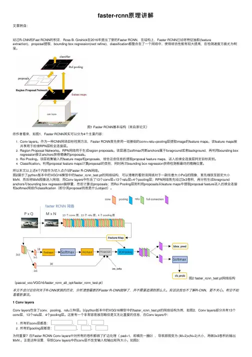
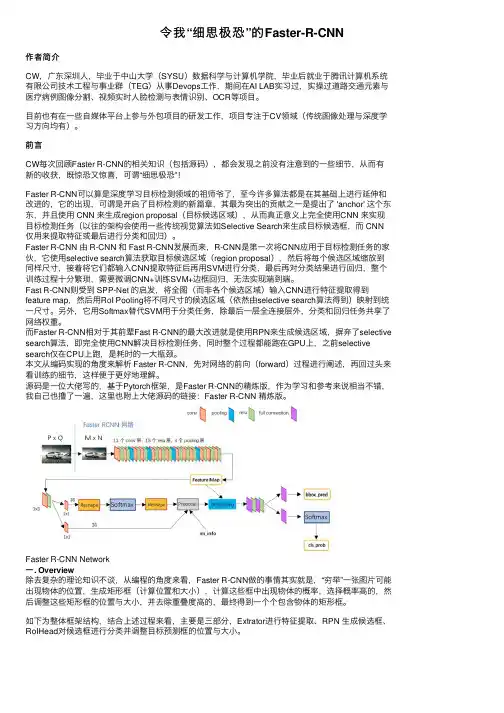
faster-rcnn原理讲解⽂章转⾃:经过R-CNN和Fast RCNN的积淀,Ross B. Girshick在2016年提出了新的Faster RCNN,在结构上,Faster RCNN已经将特征抽取(feature extraction),proposal提取,bounding box regression(rect refine),classification都整合在了⼀个⽹络中,使得综合性能有较⼤提⾼,在检测速度⽅⾯尤为明显。
图1 Faster RCNN基本结构(来⾃原论⽂)依作者看来,如图1,Faster RCNN其实可以分为4个主要内容:1. Conv layers。
作为⼀种CNN⽹络⽬标检测⽅法,Faster RCNN⾸先使⽤⼀组基础的conv+relu+pooling层提取image的feature maps。
该feature maps被共享⽤于后续RPN层和全连接层。
2. Region Proposal Networks。
RPN⽹络⽤于⽣成region proposals。
该层通过softmax判断anchors属于foreground或者background,再利⽤bounding boxregression修正anchors获得精确的proposals。
3. Roi Pooling。
该层收集输⼊的feature maps和proposals,综合这些信息后提取proposal feature maps,送⼊后续全连接层判定⽬标类别。
4. Classification。
利⽤proposal feature maps计算proposal的类别,同时再次bounding box regression获得检测框最终的精确位置。
所以本⽂以上述4个内容作为切⼊点介绍Faster R-CNN⽹络。
图2展⽰了python版本中的VGG16模型中的faster_rcnn_test.pt的⽹络结构,可以清晰的看到该⽹络对于⼀副任意⼤⼩PxQ的图像,⾸先缩放⾄固定⼤⼩MxN,然后将MxN图像送⼊⽹络;⽽Conv layers中包含了13个conv层+13个relu层+4个pooling层;RPN⽹络⾸先经过3x3卷积,再分别⽣成foreground anchors与bounding box regression偏移量,然后计算出proposals;⽽Roi Pooling层则利⽤proposals从feature maps中提取proposal feature送⼊后续全连接和softmax⽹络作classification(即分类proposal到底是什么object)。
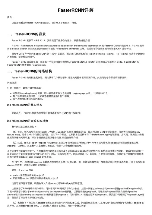
FasterRCNN详解摘⾃: 这篇是我看过讲faster-RCNN最清楚的,很多地⽅茅塞顿开,特转。
⼀、 faster-RCNN的背景 Faster R-CNN 发表于 NIPS 2015,其后出现了很多改进版本,后⾯会进⾏介绍. R-CNN - Rich feature hierarchies for accurate object detection and semantic segmentation 是 Faster R-CNN 的启发版本. R-CNN 是采⽤ Selective Search 算法来提取(propose)可能的 RoIs(regions of interest) 区域,然后对每个提取区域采⽤标准 CNN 进⾏分类. 出现于 2015 年早期的 Fast R-CNN 是 R-CNN 的改进,其采⽤兴趣区域池化(Region of Interest Pooling,RoI Pooling) 来共享计算量较⼤的部分,提⾼模型的效率. Faster R-CNN 随后被提出,其是第⼀个完全可微分的模型. Faster R-CNN 是 R-CNN 论⽂的第三个版本.R-CNN、Fast R-CNN 和Faster R-CNN 作者都有 Ross Girshick.⼆、faster-RCNN的⽹络结构 Faster R-CNN 的结构是复杂的,因为其有⼏个移动部件. 这⾥先对整体框架宏观介绍,然后再对每个部分的细节分析.问题描述:针对⼀张图⽚,需要获得的输出有:边界框(bounding boxes) 列表,即⼀幅图像有多少个候选框(region proposal),⽐如有2000个;每个边界框的类别标签,⽐如候选框⾥⾯是猫?狗?等等;每个边界框和类别标签的概率。
2.1 faster-RCNN的基本结构 除此之外,下⾯的⼏幅图也能够较好的描述发图尔-RCNN的⼀般结构:2.2 faster-RCNN的⼤致实现过程 整个⽹络的⼤致过程如下: (1)⾸先,输⼊图⽚表⽰为 Height × Width × Depth 的张量(多维数组)形式,经过预训练 CNN 模型的处理,得到卷积特征图(conv feature map)。
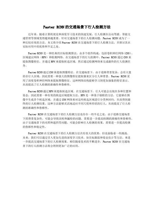
Faster RCNN的交通场景下行人检测方法近年来,随着计算机视觉和深度学习技术的快速发展,行人检测在自动驾驶、智能交通管理等领域变得越来越重要。
针对交通场景下的行人检测问题,Faster RCNN成为了一种比较有效的方法。
本文将介绍Faster RCNN在交通场景下的行人检测方法,并探讨其在实际应用中的优势和不足之处。
Faster RCNN是一种经典的目标检测算法,由多个组件构成,包括卷积神经网络(CNN)、区域建议网络(RPN)和检测网络。
在交通场景下的行人检测中,Faster RCNN通过CNN来提取图像特征,并通过RPN来提取候选区域,然后通过检测网络来完成最终的行人检测任务。
Faster RCNN通过CNN来提取图像特征。
在交通场景下,由于道路背景复杂,会有大量的非行人区域,因此需要一种强大的图像特征提取器来区分行人和背景。
Faster RCNN采用了深度卷积神经网络来提取图像特征,这种网络结构能够学习到更加抽象的特征表示,从而提高了行人检测的准确性和鲁棒性。
Faster RCNN通过RPN来提取候选区域。
在交通场景下,行人可能会出现在各种位置和姿态,因此需要一种有效的候选区域提取方法。
RPN是一种基于锚框的方法,它能够在图像中生成多个候选区域,并通过CNN网络来对这些候选区域进行分类和回归,从而得到最终的行人检测结果。
这种方法能够灵活地适应不同尺度和形状的行人,从而提高了行人检测的准确性和鲁棒性。
Faster RCNN在交通场景下的行人检测方法也存在一些不足之处。
由于道路交通场景下的背景复杂性,可能会导致误检和漏检的问题,需要进一步提高检测的准确性和鲁棒性。
由于交通场景下的光照和遮挡等问题,可能会影响行人检测的效果,需要进一步提高检测的鲁棒性和稳定性。
Faster RCNN在交通场景下的行人检测方法具有很大的优势,但也面临着一些挑战。
未来,我们可以通过引入更加先进的深度学习技术,如目标跟踪和姿态估计等方法,来进一步提高交通场景下的行人检测效果。
计算机视觉技术中常见的目标检测算法在计算机视觉领域中,目标检测是一项重要的任务,旨在从图像或视频中准确地识别和定位出特定的目标。
随着计算机技术的快速发展,目标检测算法也在不断进步和演变。
本文将介绍一些计算机视觉技术中常见的目标检测算法。
1. R-CNN(区域卷积神经网络)R-CNN是目标检测算法中的经典方法之一。
它采用两步策略来解决目标检测问题。
首先,使用选择性搜索算法生成可能包含目标的候选区域。
然后,将这些候选区域输入卷积神经网络(CNN)进行特征提取和分类。
R-CNN通过使用CNN提取图像特征,相比传统方法具有更高的准确性。
2. Fast R-CNN(快速区域卷积神经网络)Fast R-CNN是对R-CNN算法的改进。
它引入了感兴趣区域池化(RoI pooling)层,将不同大小的感兴趣区域统一为固定大小的特征向量。
这种池化操作在计算效率上具有优势,并使得Fast R-CNN比R-CNN更快速、更准确。
3. Faster R-CNN(更快速的区域卷积神经网络)Faster R-CNN是在Fast R-CNN的基础上进一步优化的算法。
它引入了候选区域生成网络(Region Proposal Network,RPN),用于自动化地生成候选区域。
通过共享特征提取和候选区域生成的过程,Faster R-CNN实现了端到端的目标检测。
相较于R-CNN和Fast R-CNN,它在准确性和速度上都有了显著的提升。
4. YOLO(你只需学会一个目标检测算法)YOLO是一种实时目标检测算法,其特点在于速度快、准确性高。
YOLO将目标检测问题转化为一个回归问题,通过在图像网格中预测边界框的坐标和类别,实现对目标的检测和分类。
YOLO算法的优点在于快速、简单,适用于实时应用。
5. SSD(单发多框检测器)SSD是一种基于卷积神经网络的目标检测算法,其主要思想是在不同尺度上检测目标。
SSD通过在不同层的特征图上应用不同大小的卷积核,实现对不同尺度目标的检测。
常用目标检测算法比较目标检测是计算机视觉领域中的一个重要任务,它可以在图片或视频中检测出物体的位置和类别。
目标检测算法可以分为两类:基于区域提取的方法和基于全卷积网络的方法。
下面将介绍常用的目标检测算法及其优缺点。
基于区域提取的方法1. R-CNN系列算法R-CNN是基于区域提取的方法的代表作之一,它通过候选区域提取算法得到候选区域,并使用卷积神经网络提取特征。
R-CNN的缺点是速度慢,需要逐个处理每个候选区域。
2. Fast R-CNNFast R-CNN在R-CNN的基础上做了改进,它将卷积神经网络应用于整张图片,得到一张特征图,然后对候选区域进行池化操作,得到固定大小的特征向量。
Fast R-CNN的速度比R-CNN提高了数十倍,但仍然比较慢。
3. Faster R-CNNFaster R-CNN是在Fast R-CNN的基础上引入了区域生成网络(Region Proposal Network,简称RPN),用于生成候选框。
Faster R-CNN比Fast R-CNN更快,精度也更高。
基于全卷积网络的方法1. YOLO系列算法YOLO(You Only Look Once)是一种基于全卷积网络的目标检测算法,它能够在一次前向传播中检测出图片中的所有物体,并且速度非常快。
但它的缺点是定位精度不高,对小物体的检测效果不好。
2. SSD系列算法SSD(Single Shot MultiBox Detector)也是一种基于全卷积网络的目标检测算法,它通过在网络不同层次上预测不同尺度的物体,并采用了多个不同尺度的先验框来检测不同大小的物体。
SSD比YOLO 的检测精度更高,但速度稍慢。
综上所述,目标检测算法因其不同的特点和应用场景而各有优劣,选择适合自己应用场景的算法是非常重要的。
图像识别技术的对比:YOLO和Faster R-CNN 图像识别技术是计算机视觉领域的一个重要研究方向,旨在通过算法和模型识别以及理解图像中的对象和内容。
在图像识别技术中,YOLO(You Only Look Once)和Faster R-CNN(Region-based Convolutional Neural Networks)是两种常用的目标检测算法,它们在实际应用中具有广泛的应用。
本文将对YOLO和Faster R-CNN进行对比,从算法原理、性能指标、优缺点等方面进行综合分析。
1.算法原理YOLO算法是一种基于卷积神经网络(CNN)的目标检测算法,它将目标检测任务视为一个回归问题,通过单个CNN模型直接在图像上进行检测和定位。
YOLO算法将图像划分为网格,并在每个网格单元中预测目标的类别和边界框,因此其算法速度较快。
而Faster R-CNN算法则采用两阶段检测框架,首先通过区域建议网络(RPN)生成候选区域,然后再对候选区域进行分类和定位。
Faster R-CNN算法通过引入RPN网络,使得检测精度和效率得到了显著提升。
2.性能指标在目标检测任务中,常用的性能指标包括准确率(Precision)、召回率(Recall)和平均精度(Average Precision)。
通过比较不同算法在这些指标上的表现,可以客观评估算法的性能。
研究表明,YOLO算法在检测速度上具有一定优势,但在目标定位和小目标检测上表现较弱;而Faster R-CNN算法在目标定位和小目标检测上有着较好的表现,但相对较慢。
3.算法优缺点YOLO算法的优点在于检测速度快,实时性好,在对大型目标进行检测时具有一定优势。
然而,YOLO算法在小物体检测和目标定位方面表现较差,容易出现目标漏检和定位偏差的情况。
而Faster R-CNN算法的优点在于检测精度高,可以有效识别小物体和进行精确的目标定位;但其缺点是算法速度较慢,对实时性要求较高的应用场景不太适用。
fasterrcnn损失函数Faster R-CNN是一种流行的目标检测算法,其损失函数主要由两部分组成:分类损失和回归损失。
1.分类损失:在Faster R-CNN中,分类任务的损失函数采用交叉熵损失函数。
分类损失的目标是根据物体的特征将其正确地分类为不同的类别。
具体而言,对于每个RoI(Region of Interest,感兴趣区域),将其特征向量输入全连接层进行线性变换,然后通过Softmax函数进行归一化,得到各个类别的概率分布。
分类损失函数如下所示:L_cls = - ∑ (y_i * log(p_i))2.回归损失:另一方面,Faster R-CNN中还设计了一种回归损失函数,用于根据候选框的位置信息来精确定位物体。
回归损失是通过计算预测的候选框和真实候选框之间的差异来定义的。
具体而言,对于每个候选框,首先通过回归层对其位置进行线性变换,得到预测的候选框位置。
然后,计算预测候选框与真实候选框之间的差异。
回归损失函数如下所示:L_reg = ∑ (smooth_L1(t_i - t*_i))其中,t_i表示真实候选框的位置,t*_i表示预测候选框的位置,smooth_L1表示平滑L1损失函数。
该损失函数可以使得预测候选框的位置和真实候选框的位置之间的平均绝对误差最小化。
综合以上两个损失函数,Faster R-CNN的总损失函数可以定义为:L_total = L_cls + λ * L_reg其中,L_cls代表分类损失,L_reg代表回归损失,λ是一个可调参数用于平衡两个损失的权重。
通过最小化总损失函数,可以同时优化分类和定位的性能。
需要注意的是,Faster R-CNN还引入了一个辅助损失函数用于训练候选框的生成网络(Region Proposal Network,RPN)。
RPN的损失函数与回归损失函数类似,有助于更好地生成候选框。
整体而言,Faster R-CNN的损失函数是通过多任务学习来同时优化分类、定位和候选框生成的性能。
Faster RCNN的交通场景下行人检测方法一、图像数据集的获取与预处理为了训练和测试Faster RCNN模型,需要收集大量的交通场景图像数据集,并对图像进行预处理。
交通场景中的图像通常会受到光照、天气、道路状况等因素的影响,因此需要对图像进行增强和标注。
增强可以提高模型的鲁棒性和泛化能力,标注则是为了训练模型提供准确的标签信息。
在图像增强方面,可以使用一些技术如镜像翻转、随机裁剪、旋转、缩放等方法来扩充数据集。
这样可以增加训练集的多样性,提高模型的鲁棒性。
还需要对图像进行标注,即给图像中的行人标注出bounding box的位置。
这一步通常需要人工操作,可以借助一些标注工具来进行辅助标注。
二、特征提取和区域建议网络在Faster RCNN中,首先需要对图像进行特征提取,然后使用区域建议网络来生成候选框。
在交通场景下,行人通常会出现在人行道、十字路口等特定位置,因此需要对图像中的这些位置进行有效的提取。
特征提取通常使用预训练的深度卷积神经网络,如VGG16、ResNet等,来提取图像的特征。
这些网络在大规模图像数据上进行了训练,能够有效地提取出图像的高级语义特征。
然后,使用这些特征来训练区域建议网络,生成候选框。
区域建议网络会对图像进行滑动窗口操作,并计算每个窗口中是否存在目标(行人)的概率以及边界框的位置。
三、目标检测和后处理在得到了候选框之后,接下来就是进行目标检测和后处理。
对于交通场景下的行人检测,需要使用分类器对每个候选框进行分类,并使用回归器来调整框的位置。
需要对检测结果进行后处理,剔除重叠框和低置信度的框。
在Faster RCNN中,通常使用softmax分类器对每个候选框进行分类,并使用回归器对边界框进行调整。
分类器可以判断出每个候选框中是否包含行人,回归器则可以对候选框的位置做出微调。
然后,使用非极大值抑制(Non-Maximum Suppression,简称NMS)来剔除重叠的框和低置信度的框,得到最终的行人检测结果。
Faster-RCNN流程RPN概述1) RPN⽹络综述Base Model最后⼀层经过⼀个3*3*512的卷积后,分两路,⼀路为1*1*18卷积,代表每个点9个anchor,2类(fg和bg),因此是9*2=18维2分类预测值;另⼀路为1*1*36,代表每个点9个anchor,4个坐标值(x,y,w,h),因此是9*436维坐标值预测。
输⼊图像320*240的情况下,卷积到3*3后的feature map⼤⼩H=36,W=61,每个点9个anchor,也就是36*61*9=19764,⼤约2W个anchor。
2) RPN⽹络中AnchorTargetCreator分析:将2W个候选anchor选出256个anchor进⾏⼆分类和所有的anchor进⾏位置回归。
为上⾯的预测值提供相应的真实值。
选择⽅式如下:对于每⼀个ground truth bouding box(gt_bbox), 选择和它IoU最⾼的⼀个anchor作为正样本。
对于剩下的anchor,从中选择和任意⼀个gt_bbox重叠度超过0.7的anchor,作为正样本,正样本的数⽬不超过128个。
随机选择和gt_bbox重叠度⼩于0.3的anchor作为负样本。
负样本和正样本的总数为256.对于每个anchor,gt_label要么为1(fg),要么为0(bg),所以这样实现⼆分类。
在计算回归损失的时候,只计算正样本(fg)的损失,不计算负样本的位置损失。
3) RPN⽹络中ProposalCreator分析:RPN利⽤AnchorTargetCreator⾃⾝训练的同时,还会提供RoIs(region of interests)给Fast RCNN(RoIHead)作为训练样本。
RPN⽣成RoIs的过程(ProposalCreator)如下:对于每张图⽚,利⽤它的feature map, 计算(H/16)*(W/16)*9(⼤概2W)个anchor属于前景的概率,以及对应的位置参数。
Faster R-CNN:Towards Real-Time Object Detectionwith Region Proposal NetworksShaoqing Ren ∗Kaiming HeRoss Girshick Jian SunMicrosoft Research{v-shren,kahe,rbg,jiansun }@AbstractState-of-the-art object detection networks depend on region proposal algorithms to hypothesize object locations.Advances like SPPnet [7]and Fast R-CNN [5]have reduced the running time of these detection networks,exposing region pro-posal computation as a bottleneck.In this work,we introduce a Region Proposal Network (RPN)that shares full-image convolutional features with the detection network,thus enabling nearly cost-free region proposals.An RPN is a fully-convolutional network that simultaneously predicts object bounds and objectness scores at each position.RPNs are trained end-to-end to generate high-quality region proposals,which are used by Fast R-CNN for detection.With a simple alternating optimization,RPN and Fast R-CNN can be trained to share convolu-tional features.For the very deep VGG-16model [18],our detection system has a frame rate of 5fps (including all steps )on a GPU,while achieving state-of-the-art object detection accuracy on PASCAL VOC 2007(73.2%mAP)and 2012(70.4%mAP)using 300proposals per image.The code will be released.1IntroductionRecent advances in object detection are driven by the success of region proposal methods (e.g.,[21])and region-based convolutional neural networks (R-CNNs)[6].Although region-based CNNs were computationally expensive as originally developed in [6],their cost has been drastically reduced thanks to sharing convolutions across proposals [7,5].The latest incarnation,Fast R-CNN [5],achieves near real-time rates using very deep networks [18],when ignoring the time spent on region proposals .Now,proposals are the computational bottleneck in state-of-the-art detection systems.Region proposal methods typically rely on inexpensive features and economical inference schemes.Selective Search (SS)[21],one of the most popular methods,greedily merges superpixels based on engineered low-level features.Yet when compared to efficient detection networks [5],Selective Search is an order of magnitude slower,at 2s per image in a CPU implementation.EdgeBoxes [23]currently provides the best tradeoff between proposal quality and speed,at 0.2s per image.Nevertheless,the region proposal step still consumes as much running time as the detection network.One may note that fast region-based CNNs take advantage of GPUs,while the region proposal meth-ods used in research are implemented on the CPU,making such runtime comparisons inequitable.An obvious way to accelerate proposal computation is to re-implement it for the GPU.This may be an effective engineering solution,but re-implementation ignores the down-stream detection network and therefore misses important opportunities for sharing computation.In this paper,we show that an algorithmic change—computing proposals with a deep net—leads to an elegant and effective solution,where proposal computation is nearly cost-free given the de-tection network’s computation.To this end,we introduce novel Region Proposal Networks (RPNs)∗Shaoqing Ren is with the University of Science and Technology of China.This work was done when he was an intern at Microsoft Research.a r X i v :1506.01497v 1 [c s .C V ] 4 J u n 2015that share convolutional layers with state-of-the-art object detection networks[7,5].By sharing convolutions at test-time,the marginal cost for computing proposals is small(e.g.,10ms per image). Our observation is that the convolutional(conv)feature maps used by region-based detectors,like Fast R-CNN,can also be used for generating region proposals.On top of these conv features, we construct RPNs by adding two additional convolutional layers:one that encodes each conv map position into a short(e.g.,256-d)feature vector and a second that,at each conv map position,outputs an objectness score and regressed bounds for k region proposals relative to various scales and aspect ratios at that location(k=9is a typical value).Our RPNs are thus a kind of fully-convolutional network(FCN)[13]and they can be trained end-to-end specifically for the task for generating detection proposals.To unify RPNs with Fast R-CNN[5] object detection networks,we propose a simple training scheme that alternates betweenfine-tuning for the region proposal task and thenfine-tuning for object detection,while keeping the proposals fixed.This scheme converges quickly and produces a unified network with convolutional features that are shared between both tasks.We evaluate our method on the PASCAL VOC detection benchmarks[4],where RPNs with Fast R-CNNs produce detection accuracy better than the strong baseline of Selective Search with Fast R-CNNs.Meanwhile,our method waives nearly all computational burdens of SS at test-time—the effective running time for proposals is ing the expensive very deep models of[18],our detection method still has a frame rate of5fps(including all steps)on a GPU,and thus is a practical object detection system in terms of both speed and accuracy(73.2%mAP on PASCAL VOC2007and70.4%mAP on2012).The code will be released.2Related WorkSeveral recent papers have proposed ways of using deep networks for locating class-specific or class-agnostic bounding boxes[20,17,3,19].In the OverFeat method[17],a4-d output fc layer (for each or all classes)is trained to predict the box coordinates for the localization task(which assumes a single object).The fc layer is then turned into a conv layer for detecting multiple class-specific objects.The MultiBox methods[3,19]generate region proposals from a network whose last fc layer simultaneously predicts multiple(e.g.,800)boxes,which are used for R-CNN[6]object detection.Their proposal network is applied on a single image or multiple large image crops(e.g., 224×224)[19].We discuss OverFeat and MultiBox in more depth later in context with our method. Shared computation of convolutions[17,7,2,5]has been attracting increasing attention for efficient, yet accurate,visual recognition.The OverFeat paper[17]computes conv features from an image pyramid for classification,localization,and detection.Adaptively-sized pooling[7]on shared conv feature maps is proposed for efficient region-based object detection[7,15]and semantic segmenta-tion[2].Fast R-CNN[5]enables end-to-end training of adaptive pooling on shared conv features and shows compelling accuracy and speed.3Region Proposal NetworksA Region Proposal Network(RPN)takes an image(of any size)as input and outputs a set of rectangular object proposals,each with an objectness score.1We model this process with a fully-convolutional network[13],which we describe in this section.Because our ultimate goal is to share computation with a Fast R-CNN object detection network[5],we assume that both nets share a common set of conv layers.In our experiments,we investigate the Zeiler and Fergus model[22] (ZF),which has5shareable conv layers and the Simonyan and Zisserman model[18](VGG),which has13shareable conv layers.To generate region proposals,we slide a small network over the conv feature map output by the last shared conv layer.This network is fully connected to an n×n spatial window of the input conv feature map.Each sliding window is mapped to a lower-dimensional vector(256-d for ZF and512-d for VGG).This vector is fed into two sibling fully-connected layers—a box-regression layer(reg) 1“Region”is a generic term and in this paper we only consider rectangular regions,as is common for many methods(e.g.,[19,21,23]).“Objectness”measures membership to a set of object classes vs.background.conv feature mapintermediate layer256-d2kscores 4k coordinatessliding windowreg layerclslayerk anchorboxesbus :0.996person :0.736Figure 1:Left :Region Proposal Network (RPN).Right :Example detections using RPN proposals on PASCAL VOC 2007test.Our method detects objects in a wide range of scales and aspect ratios.and a box-classification layer (cls ).We use n =3in this paper,noting that the effective receptive field on the input image is large (171and 228pixels for ZF and VGG,respectively).This mini-network is illustrated at a single position in Fig.1(left).Note that because the mini-network operates in a sliding-window fashion,the fully-connected layers are shared across all spatial locations.This architecture is naturally implemented with an n ×n conv layer followed by two sibling 1×1conv layers (for reg and cls ,respectively).ReLUs [14]are applied to the output of the n ×n conv layer.Translation-Invariant AnchorsAt each sliding-window location,we simultaneously predict k region proposals,so the reg layer has 4k outputs encoding the coordinates of k boxes.The cls layer outputs 2k scores that estimate probability of object /not-object for each proposal.2The k proposals are parameterized relative to k reference boxes,called anchors .Each anchor is centered at the sliding window in question,and is associated with a scale and aspect ratio.We use 3scales and 3aspect ratios,yielding k =9anchors at each sliding position.For a conv feature map of a size W ×H ,there are W Hk anchors in total.An important property of our approach is that it is translation invariant ,both in terms of the anchors and the functions that compute proposals relative to the anchors.As a comparison,the MultiBox method [19]uses k-means to generate 800anchors,which are not translation invariant.If one translates an object in an image,the proposal should translate and the same function should be able to predict the proposal in either location.Moreover,because the MultiBox anchors are not translation invariant,it requires a (4+1)×800-dimensional output layer,whereas our method requires a (4+2)×9-dimensional output layer.Our proposal layers have an order of magnitude fewer parameters (27million for MultiBox using GoogLeNet [19]vs.2.4million for RPN using VGG-16),and thus have less risk of overfitting on small datasets,like PASCAL VOC.A Loss Function for Learning Region ProposalsFor training RPNs,we assign a binary class label (of being an object or not)to each anchor.We assign a positive label to two kinds of anchors:(i)the anchor that has the highest Intersection-over-Union (IoU)overlap with a ground-truth box,or (ii)an anchor that has an IoU overlap higher than 0.7with any ground-truth box.3Note that a single ground-truth box may assign positive labels to multiple anchors.We assign a negative label to a non-positive anchor if its IoU ratio is lower than 0.3for all ground-truth boxes.There are anchors that are neither positive nor negative,and they are ignored and will not contribute to the training objective.With these definitions,we minimize an objective function following the multi-task loss in Fast R-CNN [5].For an anchor box i ,its loss function is defined as:L (p i ,t i )=L cls (p i ,p ∗i )+λp ∗i L reg (t i ,t ∗i ).(1)2For simplicity we implement the cls layer as a two-class softmax layer.Alternatively,one may use logisticregression to produce k scores.3We intend to simplify this to case (ii),only.Current experiments,however,consider an anchor as positive if it satisfies condition (i)or condition (ii).Here p i is the predicted probability of the anchor i being an object.p∗i is1if the anchor is labeled positive,and is0if the anchor is negative.t i={t x,t y,t w,t h}i represents the4parameterizedcoordinates of the predicted bounding box,and t∗i={t∗x,t∗y,t∗w,t∗h }i represents the ground-truthbox associated with a positive anchor.The classification loss L cls is the softmax loss of two classes (object vs.not object).For the regression loss,we use L reg(t i,t∗i)=R(t i−t∗i)where R is the robust loss function(smooth-L1)defined in[5].The term p∗i L reg means the regression loss is activated only for positive anchors(p∗i=1)and is disabled otherwise(p∗i=0).The loss-balancing parameterλis set to10,which means that we bias towards better box locations.The outputs of the cls and reg layers consist of{p i}and{t i}respectively.We adopt the parameterizations of the4coordinates following[6]:t x=(x−x a)/w a,t y=(y−y a)/h a,t w=log(w/w a),t h=log(h/h a) t∗x=(x∗−x a)/w a,t∗y=(y∗−y a)/h a,t∗w=log(w∗/w a),t∗h=log(h∗/h a),where x,x a,and x∗are for the predicted box,anchor box,and ground-truth box respectively.This can be thought of as bounding-box regression from an anchor box to a nearby ground-truth box. Nevertheless,our method achieves bounding-box regression by a different manner from previous feature-map-based methods[7,5].In[7,5],bounding-box regression is performed on features pooled from arbitrarily sized regions,and the regression weights are shared by all region sizes.In our formulation,the features used for regression are of the same spatial size(n×n)on the feature maps.To account for varying sizes,a set of k bounding-box regressors are learned.Each regressor is responsible for one scale and one aspect ratio,and the k regressors do not share weights.As such, it is still possible to predict boxes of various sizes even though the features are of afixed size/scale. OptimizationThe RPN,which is naturally implemented as a fully-convolutional network[13],can be trained end-to-end by back-propagation and stochastic gradient descent(SGD)[12].We follow the“image-centric”sampling strategy from[5]to train this network.Each mini-batch arises from a single image that contains many positive and negative examples.It is possible to optimize for the loss functions of all anchors,but this will bias towards negative samples as they are dominate.Instead,we randomly sample256anchors in an image to compute the loss function of a mini-batch,where the sampled positive and negative anchors have a ratio of1:1.We randomly initialize all new layers by drawing weights from a zero-mean Gaussian distribution with standard deviation0.01.All other layers(i.e.,the shared conv layers)are initialized by pre-training a model for ImageNet classification[16],as is standard practice[6].We tune all layers of the ZF net,and conv31and up for the VGG net to conserve memory[5].We use a learning rate of 0.001for60k mini-batches,and0.0001for the next20k mini-batches on the PASCAL dataset.We also use a momentum of0.9and a weight decay of0.0005[11].We implement in Caffe[10]. Sharing Convolutional Features for Region Proposal and Object DetectionThus far we have described how to train a network for region proposal generation,without con-sidering the region-based object detection CNN that will utilize these proposals.For the detection network,we adopt Fast R-CNN[5]4and now describe an algorithm that learns conv layers that are shared between the Region Proposal Network and Fast R-CNN.Both RPN and Fast R-CNN,trained independently,will modify their conv layers in different ways. We therefore need to develop a technique that allows for sharing conv layers between the two net-works,rather than learning two separate networks.Note that this is not as easy as simply defining a single network that includes both RPN and Fast R-CNN,and then optimizing it jointly with back-propagation.The reason is that Fast R-CNN training depends onfixed object proposals and it is not clear a priori if learning Fast R-CNN while simultaneously changing the proposal mechanism will converge.While this joint optimizing is an interesting question for future work,we develop a pragmatic4-step training algorithm to learn shared features via alternating optimization.In thefirst step,we train the RPN as described above.This network is initialized with an ImageNet-pre-trained model andfine-tuned end-to-end for the region proposal task.In the second step,wetrain a separate detection network by Fast R-CNN using the proposals generated by the step-1RPN. This detection network is also initialized by the ImageNet-pre-trained model.At this point the two networks do not share conv layers.In the third step,we use the detector network to initialize RPN training,but wefix the shared conv layers and onlyfine-tune the layers unique to RPN.Now the two networks share conv layers.Finally,keeping the shared conv layersfixed,wefine-tune the fc layers of the Fast R-CNN.As such,both networks share the same conv layers and form a unified network. Implementation DetailsWe train and test both region proposal and object detection networks on single-scale images[7, 5].We re-scale the images such that their shorter side is s=600pixels[5].Multi-scale feature extraction may improve accuracy but does not exhibit a good speed-accuracy trade-off[5].For anchors,we use3scales with box areas of1282,2562,and5122pixels,and3aspect ratios of 1:1,1:2,and2:1.We note that our algorithm allows use of anchor boxes that are larger than the underlying receptivefield when predicting large proposals.Such predictions are not impossible—one may still roughly infer the extent of an object if only the middle of the object is visible.With this design,our solution does not need multi-scale features or multi-scale sliding windows to predict large regions,saving considerable running time.Fig.1(right)shows the capability of our method for a wide range of scales and aspect ratios.The table below shows the learned average proposal size for each anchor using the ZF net(numbers for s=600).anchor1282,2:11282,1:11282,1:22562,2:12562,1:12562,1:25122,2:15122,1:15122,1:2 proposal188×111113×11470×92416×229261×284174×332768×437499×501355×715The anchor boxes that cross image boundaries need to be handled with care.During training,we ignore all cross-boundary anchors,and they will not contribute to the loss.For a typical1000×600 image,there will be roughly20k(≈60×40×9)anchors in total.With the cross-boundary anchors ignored,there are about6k anchors per image for training.If the outliers are not ignored in training, they introduce large,difficult to correct error terms in the objective function,and training does not converge.During testing,however,we still apply the fully-convolutional RPN to the entire image. This may generate cross-boundary proposal boxes,which we clip to the image boundary.Some RPN proposals highly overlap with each other.To reduce redundancy,we adopt non-maximum suppression(NMS)on the proposal regions based on their cls scores.Wefix the IoU threshold for NMS at0.7,which leaves us about2k proposal regions per image.As we will show, NMS does not harm the ultimate detection accuracy,but substantially reduces the number of pro-posals.After NMS,we use the top-N ranked proposal regions for detection.In the following,we train Fast R-CNN using2k RPN proposals,but evaluate different numbers of proposals at test-time. 4ExperimentsWe comprehensively evaluate our method on the PASCAL VOC2007detection benchmark[4]. This dataset consists of about5k trainval images and5k test images over20object categories.We also provide results in the PASCAL VOC2012benchmark for a few models.For the ImageNet pre-trained network,we use the“fast”version of ZF net[22]that has5conv layers and3fc layers, and the public VGG-16model5[18]that has13conv layers and3fc layers.We primarily evalu-ate detection mean Average Precision(mAP),because this is the actual metric for object detection (rather than focusing on object proposal proxy metrics).Table1(top)shows Fast R-CNN results when trained and tested using various region proposal methods.These results use the ZF net.For Selective Search(SS)[21],we generate about2k SS proposals by the“fast”mode.For EdgeBoxes(EB)[23],we generate the proposals by the default EB setting tuned for0.7IoU.SS has an mAP of58.7%and EB has an mAP of58.6%.RPN with Fast R-CNN achieves competitive results,with an mAP of59.9%while using ing RPN for proposals and limiting Fast R-CNN to the top300regions yields a much faster detector than using either SS or EB.Next,we consider several ablations of RPN and then show that proposal quality improves when using the very deep VGG-16network.Table1:Detection results on PASCAL VOC2007test set(trained on VOC2007trainval).The detectors are Fast R-CNN with ZF,but using various proposal methods for training and testing.train-time region proposals test-time region proposalsmethod#boxes method#proposals mAP(%)SS2k SS2k58.7EB2k EB2k58.6RPN+ZF,shared2k RPN+ZF,shared30059.9ablation experiments follow belowRPN+ZF,unshared2k RPN+ZF,unshared30058.7SS2k RPN+ZF10055.1SS2k RPN+ZF30056.8SS2k RPN+ZF1k56.3SS2k RPN+ZF(no NMS)6k55.2SS2k RPN+ZF(no cls)10044.6SS2k RPN+ZF(no cls)30051.4SS2k RPN+ZF(no cls)1k55.8SS2k RPN+ZF(no reg)30052.1SS2k RPN+ZF(no reg)1k51.3SS2k RPN+VGG30059.2Ablation Experiments.To investigate the behavior of RPNs as a proposal method,we conducted several ablation studies.First,we show the effect of sharing conv layers between the RPN and Fast R-CNN detection network.To do this,we stop after the second step in the4-step training process. Using separate networks reduces the result slightly to58.7%(RPN+ZF,unshared,Table1).We observe that this is because in the third step when the detector-tuned features are used tofine-tune the RPN,the proposal quality is improved.Next,we disentangle the RPN’s influence on training the Fast R-CNN detection network.For this purpose,we train a Fast R-CNN model by using the2k SS proposals and ZF net.Wefix this detector and evaluate the detection mAP by changing the proposal regions used at test-time.In these ablation experiments,the RPN does not share features with the detector.Replacing SS with300RPN proposals at test-time leads to an mAP of56.8%.The loss in mAP is because of the inconsistency between the training/testing proposals.This result serves as the baseline for the following comparisons.Somewhat surprisingly,the RPN still leads to a competitive result(55.1%)when using the top-ranked100proposals at test-time,indicating that the top-ranked RPN proposals are accurate.On the other extreme,using the top-ranked6k RPN proposals(without NMS)has a comparable mAP (55.2%),suggesting NMS does not harm the detection mAP and may reduce false alarms.Next,we separately investigate the roles of RPN’s cls and reg outputs by turning off either of them at test-time.When the cls layer is removed at test-time(thus no NMS/ranking is used),we randomly sample N proposals from the unscored regions.The mAP is nearly unchanged with N=1k (55.8%),but degrades considerably to44.6%when N=100.This shows that the cls scores account for the accuracy of the highest ranked proposals.On the other hand,when the reg layer is removed at test-time(so the proposals become anchor boxes),the mAP drops to52.1%.This suggests that the high-quality proposals are mainly due to regressed positions.The anchor boxes alone are not sufficient for accurate detection.We also evaluate the effects of more powerful networks on the proposal quality of RPN alone. We use VGG-16to train the RPN,and still use the above detector of SS+ZF.The mAP improves from56.8%(using RPN+ZF)to59.2%(using RPN+VGG).This is a promising result,because it suggests that the proposal quality of RPN+VGG is better than that of RPN+ZF.Because proposals of RPN+ZF are competitive with SS(both are58.7%when consistently used for training and testing), we may expect RPN+VGG to be better than SS.The following experiments justify this hypothesis.Table2:Detection results on PASCAL VOC2007test set.The detector is Fast R-CNN and VGG-16.Training data:“07”:VOC2007trainval,“07+12”:union set of VOC2007trainval and VOC 2012trainval.For RPN,the train-time proposals for Fast R-CNN are2k.method#proposals data mAP(%)time(ms)SS2k0766.91830SS2k07+1270.01830RPN+VGG,unshared3000768.5342RPN+VGG,shared3000769.9196RPN+VGG,shared30007+1273.2196Table3:Detection results on PASCAL VOC2012test set.The detector is Fast R-CNN and VGG-16.Training data:“07”:VOC2007trainval,“07++12”:union set of VOC2007trainval+test and VOC2012trainval.For RPN,the train-time proposals for Fast R-CNN are2k.†:http:// :8080/anonymous/HZJTQA.html.‡::8080/ anonymous/YNPLXB.htmlmethod#proposals data mAP(%)SS2k1265.7SS2k07++1268.4RPN+VGG,shared†3001267.0RPN+VGG,shared‡30007++1270.4Table4:Timing(ms)on an Nvidia K40GPU evaluated in Caffe[10],except SS proposal is evalu-ated in a CPU.The region-wise computation includes NMS,pooling,fc,softmax,and others.model system conv proposal region-wise total rateVGG SS+Fast R-CNN146151017418300.5fpsVGG RPN+Fast R-CNN14610401965fpsZF RPN+Fast R-CNN373286815fpsDetection Accuracy and Running Time of VGG-16.Table2shows the results of VGG-16for both proposal and detection.The Fast R-CNN baseline of SS and VGG-16has an mAP of66.9% [5].Using RPN+VGG,the Fast R-CNN result is68.5%for unshared features,1.6%higher than the SS baseline.As shown above,this is because the proposals generated by RPN+VGG are more accurate than SS.Unlike SS that is pre-defined,the RPN is actively trained and benefits from better networks.For the feature-shared variant,the result is69.9%—better than the strong SS baseline, yet with nearly cost-free proposals.We further train the RPN and detection network on the union set of PASCAL VOC2007trainval and2012trainval,following[5].The mAP is73.2%,which is 3.2%higher than the SS counterpart.On the PASCAL VOC2012test set(Table3),our method has an mAP of70.4%trained on the union set of VOC2007trainval+test and VOC2012trainval, following[5].This is2.0%higher than the SS counterpart.In Table4we summarize the running time of the entire object detection system.SS takes1-2 seconds depending on content(on average1.51s),and Fast R-CNN with VGG-16takes320ms on 2k SS proposals(or223ms if using SVD on fc layers[5]).Our system with VGG-16takes in total 196ms for both proposal and detection.With the conv features shared,the RPN alone only takes 10ms computing the additional layers.Our region-wise computation is also low,thanks to fewer proposals(300).Our system has a rate of15fps with the ZF net.Analysis of Recall-to-IoU.Next we compute the recall of proposals at different IoU ratios with ground-truth boxes.It is noteworthy that the Recall-to-IoU metric is just loosely[9,8,1]related to the ultimate detection accuracy.It is more appropriate to use this metric to diagnose the proposal method than to evaluate it.In Fig.2,we show the results of using300,1k,and2k proposals.We compare with SS and EB,and the N proposals are the top-N ranked ones based on the confidence generated by these methods. The plots show that the RPN method behaves gracefully when the number of proposals drops from 2k to300.This explains why the RPN has a good ultimate detection mAP when using as few as300Figure2:Recall vs.IoU overlap ratio on the PASCAL VOC2007test set.Table5:One-Stage Detection vs.Two-Stage Proposal+Detection.Detection results are on the PASCAL VOC2007test set using the ZF model and Fast R-CNN.RPN uses unshared features.regions detector mAP(%) Two-Stage RPN+ZF,unshared300Fast R-CNN+ZF,1scale58.7One-Stage dense,3scales,3asp.ratios20k Fast R-CNN+ZF,1scale53.8One-Stage dense,3scales,3asp.ratios20k Fast R-CNN+ZF,5scales53.9 proposals.As we analyzed before,this property is mainly attributed to the cls term of the RPN.The recall of SS and EB drops more quickly than RPN when the proposals are fewer.We also notice that for high IoU ratios(e.g.,>0.8),the recall of RPN and EB is lower than that of SS,but the ultimate detection mAP is not impacted.This also suggests that the Recall-to-IoU curve is not tightly related to the detection mAP.One-Stage Detection vs.Two-Stage Proposal+Detection.The OverFeat paper[17]proposes a detection method that uses regressors and classifiers on sliding windows over conv feature maps. OverFeat is a one-stage,class-specific detection pipeline,and ours is a two-stage cascade consisting of class-agnostic proposals and class-specific detections.In OverFeat,the region-wise features come from a sliding window of one aspect ratio over a scale pyramid.These features are used to simulta-neously determine the location and category of objects.In RPN,the features are from square(3×3) sliding windows and predict proposals relative to anchors with different scales and aspect ratios. Though both methods use sliding windows,the region proposal task is only thefirst stage of RPN +Fast R-CNN—the detector attends to the proposals to refine them.In the second stage of our cas-cade,the region-wise features are adaptively pooled[7,5]from proposal boxes that more faithfully cover the features of the regions.We believe these features lead to more accurate detections.To compare the one-stage and two-stage systems,we emulate the OverFeat system(and thus also circumvent other differences of implementation details)by one-stage Fast R-CNN.In this system, the“proposals”are dense sliding windows of3scales(128,256,512)and3aspect ratios(1:1,1:2, 2:1).Fast R-CNN is trained to predict class-specific scores and regress box locations from these sliding windows.Because the OverFeat system adopts multi-scale features,we also evaluate using conv features extracted from5scales.We use those5scales as in[7,5].Table5compares the two-stage system and two variants of the one-stage ing the ZF model,the one-stage system has an mAP of53.9%.This is lower than the two-stage system(58.7%) by4.8%.This experiment justifies the effectiveness of cascaded region proposals and object detec-tion.Note that the one-stage system is also slower as it has considerably more proposals to process. 5ConclusionWe have presented Region Proposal Networks(RPNs)for efficient and accurate region proposal generation.By sharing convolutional features with the down-stream detection network,the region proposal step is nearly cost-free.Our method enables a unified,deep-learning-based object detection system to run at5-15fps.The learned RPN also improves region proposal quality and thus the overall object detection accuracy.。