Analysis of train movement dynamics in fixed-block railway network

机械运动的英语Mechanical MotionMechanical motion is a fundamental concept in physics that describes the movement of objects and the forces that govern their behavior. This form of motion is essential in various fields, from engineering and transportation to robotics and everyday life. Understanding the principles of mechanical motion is crucial for designing and analyzing a wide range of systems and devices.At its core, mechanical motion involves the displacement of an object from one point to another, often through the application of external forces. These forces can be a result of various factors, such as gravity, friction, or the action of other objects. The study of mechanical motion encompasses the analysis of the motion of rigid bodies, as well as the deformation and behavior of flexible materials.One of the key aspects of mechanical motion is the concept of kinematics, which deals with the description of motion without considering the forces that cause it. Kinematics examines the position, velocity, acceleration, and other related quantities of an object as it moves through space. This information is crucial forunderstanding the behavior of a system and predicting its future states.Another important aspect of mechanical motion is dynamics, which focuses on the forces and torques that act on an object and how they influence its motion. Dynamics provides a deeper understanding of the underlying principles that govern the movement of objects, including the conservation of energy and momentum, as well as the effects of friction and other dissipative forces.The applications of mechanical motion are vast and diverse. In engineering, the study of mechanical motion is essential for the design and analysis of mechanical systems, such as engines, gears, and robotic manipulators. In transportation, the principles of mechanical motion are used to design vehicles, predict their performance, and optimize their efficiency. In everyday life, mechanical motion is encountered in the operation of household appliances, tools, and even the human body.Advances in computational power and numerical simulations have further expanded the understanding and application of mechanical motion. Computational fluid dynamics, for example, can be used to model the complex flow of fluids and the interaction between solids and fluids, enabling the design of more efficient and optimizedsystems.Moreover, the study of mechanical motion has led to the development of innovative technologies, such as energy harvesting devices, which can convert the motion of objects into electrical energy. These advancements have the potential to contribute to the development of more sustainable and efficient energy solutions.In conclusion, the study of mechanical motion is a fundamental and multifaceted field that underpins a wide range of technological and scientific advancements. By understanding the principles of kinematics, dynamics, and the various forces that govern the movement of objects, engineers, scientists, and researchers can continue to push the boundaries of what is possible and create novel solutions to the challenges facing our world.。

对交通工程专业的理解英文作文Understanding of the Traffic Engineering SpecialtyHaving a solid understanding of the traffic engineering specialty is paramount in addressing a myriad of challenges that arise from modern transportation systems. Traffic engineering serves as the backbone for planning, designing, and implementing solutions that ensure efficient and safe movement of people, goods, and services within urban and rural areas. In essence, it encompasses a wide array of knowledge domains such as traffic flow theory, transportation planning, traffic control systems, and road infrastructure.One crucial aspect is traffic flow theory which entails comprehending the dynamics of vehicle movement. This pertains to fundamental concepts such as traffic density, speed-flow relationships, and capacity analysis. Knowledge in this area enables professionals to accurately predict traffic behavior under different conditions and develop suitable measures to alleviate congestion or improveoverall traffic efficiency.Transportation planning represents another critical facet of traffic engineering. It involves comprehensive assessments of current infrastructural capacities and anticipated future needs. By utilizing mathematical models and simulation tools, engineers can determine optimal road networks, public transit systems, and other transport facilities to maximize efficiency while minimizing environmental impact.Moreover, proficiency in traffic control systems is essential for managing vehicular movements effectively. This area involves understanding signal timings,intelligent transportation systems (ITS), roundabouts, and other means for regulating traffic flow. Additionally, knowledge in developing sustainable road infrastructure plays a crucial role in ensuring long-term functionality by considering factors such as material durability, environmental impact assessments, and cost-efficiency.Furthermore, an interdisciplinary focus on environmentalsustainability has become increasingly important within the field. Professionals in traffic engineering are expected to promote eco-friendly practices through initiatives like carpooling incentives, bike lanes construction or public transport improvement projects. Such efforts play a keyrole in reducing carbon emissions and fostering a balanced approach to urban development.Being conversant with these areas not only equips professionals with technical skills but also nurtures creativity when tackling real-world problems arising from transportation demands. Moreover, it cultivates an awareness towards the societal implications associated with urban mobility challenges – particularly related to safety concerns for pedestrians and cyclists – encouraging thorough consideration of diverse perspectives when devising solutions.In conclusion, the breadth of knowledge encompassed by the study of traffic engineering is indispensable for addressing contemporary mobility challenges faced by societies today. It extends far beyond mere asphalt andconcrete; instead encapsulating an intricate web of theories and practical applications that shape our daily commutes while fundamentally impacting environmental sustainability. Understanding this specialty involves recognizing its intrinsic importance in fostering efficient movement patterns without compromising safety or ecological well-being.。

dynamics单词意思详解## Dynamics.Dynamics is the branch of physics that deals with the forces that produce motion in objects and the effects of those forces on the objects. It is a fundamental science that has applications in many fields of science and engineering, including mechanics, astronomy, and engineering.The laws of dynamics were first developed by Isaac Newton in the late 17th century. Newton's three laws of motion describe the relationship between an object's mass, velocity, and acceleration. These laws can be used to solve a wide variety of problems involving the motion of objects.Newton's First Law of Motion.Newton's first law of motion, also known as the law of inertia, states that an object at rest will remain at rest,and an object in motion will remain in motion at a constant velocity, unless acted upon by an unbalanced force. In other words, objects have a natural tendency to resist changes in their motion.Newton's Second Law of Motion.Newton's second law of motion states that the acceleration of an object is directly proportional to the net force acting on the object, and inversely proportional to the mass of the object. This law can be expressed mathematically as:F = ma.where:F is the net force acting on the object (in newtons)。

分析广场人群数据的英语作文The analysis of crowd data in public squares has become an increasingly important field of study in recent years. As cities continue to grow and urbanization increases, understanding the movement and behavior of people in public spaces has become crucial for urban planners, event organizers, and security personnel. By collecting and analyzing data on the number of people, their flow, and their interactions, valuable insights can be gained to improve the design and management of public squares.One of the primary benefits of analyzing crowd data in public squares is the ability to optimize the use of space. By understanding the patterns of pedestrian traffic, the placement of entrances, exits, and other infrastructure can be adjusted to facilitate efficient movement and reduce congestion. This is particularly important during large events or festivals, where the influx of people can quickly overwhelm a public space if not properly managed.Through the use of various data collection methods, such as video surveillance, mobile device tracking, and manual counting,researchers can gather detailed information on the number of people in a given area, their arrival and departure times, and their movement patterns. This data can then be analyzed to identify peak times, high-traffic areas, and potential bottlenecks. Armed with this information, urban planners can make informed decisions about the layout and design of the square, ensuring that it can accommodate the needs of the people who use it.Another key aspect of crowd data analysis is the ability to understand the behavior and interactions of people within a public space. By studying how individuals and groups move through the square, interact with each other, and utilize the available amenities, researchers can gain valuable insights into the social dynamics of the space. This information can be used to enhance the overall experience for visitors, such as by providing more seating areas, improving lighting and signage, or introducing new activities and attractions.Furthermore, the analysis of crowd data can also play a crucial role in ensuring the safety and security of public spaces. By monitoring the movement and density of people, security personnel can quickly identify potential threats or areas of concern, and respond accordingly. This can be particularly important during events or demonstrations, where the risk of overcrowding or conflict is heightened.In recent years, the use of advanced technologies, such as computer vision and machine learning, has greatly enhanced the ability to collect and analyze crowd data in public squares. These technologies allow for the automated tracking and analysis of large numbers of individuals, providing real-time insights into the dynamics of the space. This information can then be used to inform decision-making and improve the overall management of the public square.Despite the many benefits of crowd data analysis, there are also some challenges and ethical considerations that must be addressed. The collection and use of personal data, such as that obtained through mobile device tracking, raises concerns about privacy and data protection. It is essential that any data collection and analysis efforts are conducted in a transparent and ethical manner, with strict safeguards in place to protect the privacy of individuals.Additionally, the interpretation of crowd data can be complex and nuanced, requiring a deep understanding of the social, cultural, and environmental factors that influence human behavior in public spaces. Researchers and urban planners must be careful to avoid drawing simplistic or biased conclusions from the data, and instead strive to develop a more holistic understanding of the dynamics at play.In conclusion, the analysis of crowd data in public squares is a powerful tool for improving the design, management, and safety of these important public spaces. By collecting and analyzing data on the movement and behavior of people, urban planners and event organizers can make more informed decisions, enhance the overall experience for visitors, and ensure the efficient and secure use of public squares. As cities continue to evolve and the demands on public spaces increase, the importance of crowd data analysis will only grow, making it an essential component of modern urban planning and management.。

英语精读Attain1.to succeed in getting sth,usually after a lot of effort(通常经过努⼒)获得，得到●Most of our students attained five‘A’grades in their exams.2.(formal)to reach a particular age, level or condition●The cheetah(猎豹) can attain speeds of up to 97 kph.Attainable 可达到的，可获得的●attainable goals/targetsAttainment(n) sth that you learned or achieved成就，造诣，获得Bourgeois1.belonging to the middle class 中产阶级的● A traditional bourgeois family2.interested mainly in possessions and social status and supporting traditional values 追求名利且平庸的，世俗的●They’ve become very bourgeois since they got married.3.Supporting the interests of capitalism 资产阶级的，资本家的Bourgeois ideology 资产阶级意识形态Bourgeois (n)pl: bourgeoisBourgeoisie(n)中产阶级CapitalistN. 1. A person who supports capitalism 资本主义者2.A person who owns or controls a lot of wealth and uses it to producemore wealth资本家Adj. Based on the principles of capitalism 资本主义的● A capitalist society/system/economyCapitalism(n[u])资本主义socialism社会主义cobwebN. A fine net of threads made by a spider to catch insects;蜘蛛⽹●Thick cobwebs hung in the dusty corners.Cobwebbed 布满蜘蛛⽹的Blow/clear the cobwebs away: to help sb start sth in a fresh,lively state of mind● A brisk walk should blow the cobwebs away.ConcealTo hide sb/sthConceal sb/sth (from sb/sth)●For a long time his death was concealed from her.●She sat down to conceal the fact that she was trembling. Concealment(n)Conception1.the process of forming an idea or a plan 构思，构想●The plan was brilliant in its conception but failed because of lack ofmoney.2.an understanding or a belief of what sth is or what sth should beConception of sth /conception that●He has no conception of how difficult life is if you’re unemployed. conservativeAdj.1.opposed to great or sudden social change;showing that you prefer traditional styles and values●The conservative views of his parents●Her style of dress was never conservative.2.connected with the British Conservative Party.保守党的●the Conservative Party 保守党3.Lower than what is probably the real amount or number 低于实际数量的，保守的●At a conservative estimate, he will be earning 50,000 dollars.N. 1.A member or supporter of the British Conservative Party2. A conservative person保守者，因循守旧者；Adv. ConservativelyN. conservatismCritic1.a person who expresses opinions about the good and bad qualities of books,music,etc.● A music/literary critic2.a person who expresses disapproval of sb/sth and talks about their bad qualities,especially publicly.●She is one of the ruling party’s most outspoken critics.Critical(adj.)Criticism(n.)Criticize(v.)CrownN.1,(the Crown)The government of a country,thought of as being represented by a king or queen王国政府，王国●Who’s appearing for the Crown in the case?1.(the crown )the position or power of a king or queen●She refused the crown.V.1. To put a crown on the head of a new king or queen as a sign of royal power.为……加冕●The prince was soon to be crowned King of England.2.crown sth (with sth)to make sth complete or perfect,especially by adding an achievement,a success,etc.●Their efforts were finally crowned with success.To crown it all: used to say that sth is the final and worst event on a series of unpleasant or annoying events.最糟糕的是●It was cold and raining,and ,to crown it all,we had to walk home.●Crown Court 刑事法庭Crowning(adj.)Departure1.the act of leaving a place;●His sudden departure threw the office into chaos.●Flights should be confirmed 48 hours before departure.2.a plane,train,etc.leaving a place at a particular time●Arrivals and departures到站和离站班次3.A departure(from sth)An action that is different from what is usual or expected背离，违反；●It was a radical departure from tradition.DeportV. to force sb to leave a country,usually because they have broken the law or because they have no legal right to be there●He was convinced of drug offences and deported.Deportation(n.) a deportation order 驱逐出境令dynamicN. 1.(dynamics) the way in which people or things behave and react to each other in a particular situation(⼈和事物)相互作⽤的⽅式，动态●The dynamics of political change 政治变化动态2.(dynamics)the science of the forces involved in movement动⼒学●Fluid dynamicsAdj. 1.forceful,and having a lot of energy● A dynamic personality2.always changing and making process 动态的emancipation1.The act or process of setting sb free or of freeing sb from restrictions●The emancipation of slavesEmancipated(adj.)Emancipate(v.)envisageV. To imagine what will happen in the future●What level of profit do you envisage?●I don’t envisage working with him again.●It is envisaged that the talks will take place in the spring.Epoch1.A period of time in history,especially one during which important events or changes happen●The death of the emperor marked the end of an epoch in thecountry’s history.2.a long period of time in the world’s history or in the earth’s development.世●Geological epochs地质世EvolveEvolve from sth (into sth)1.to develop gradually●The company has evolved into a major chemical manufacturer.2.to develop gradually over many generations from a simple form to a more complicated one.●The three species evolved from a single ancestor.Field1.an area of land in the country used for growing crops or keeping animals in, usually surrounded by a fence, etc.●People were working in the fields.2.an area of land used for the purpose mentioned● A landing field3.a large area of land covered with the thing mentioned; an area from which the thing mentioned is obtained●Gas fields4. a particular subject or activity that sb works in or is interested in famous in the field of music●This discovery has opened up a whole new field of research.5. the fact of people doing practical work or study, rather than working in a library or laboratory● a field study/investigation实地研究/调查6. an area of land used for playing a sport on● a baseball/rugby/football field7.all the people or products competing in a particular area of business⾏业●They lead the field in home entertainment systems.8. an area within which the force mentioned has an effect●an electro-magnetic field电磁场leave the field clear for sb/leave sb in possession of the field 为…的胜利铺平道路；为…的成功扫清障碍gapn.1.a space between two things or in the middle of sth, especially because there is a part missing●Leave a gap between your car and the next.2.a period of time when sth stops, or between two events● a gap in the conversation●They met again after a gap of twenty years.3.a difference that separates people, or their opinions, situation, etc.●the gap between rich and poor●the gap between theory and practice4.a space where sth is missing●His death left an enormous gap in my life.governv.1.to legally control a country or its people and be responsible for introducing new laws, organizing public services, etc.●The country is governed by elected representatives of the people.2.to control or influence sb/sth or how sth happens, functions, etc.●Prices are governed by market demand.grantv.1.to agree to give sb what they ask for, especially formal or legal permission to do sth●I was granted permission to visit the palace.2.to admit that sth is true, although you may not like or agree with it●She's a smart woman, I grant you, but she's no genius.take it for granted (that…)●I just took it for granted that he'd always be around.take sb/sth for granted●Her husband was always there and she just took him for granted. n.1.~ (to do sth)a sum of money that is given by the government or by another organization to be used for a particular purpose●student grants学⽣助学⾦gropev.1.~ (around)(for sth)to try and find sth that you cannot see, by feeling with your hands●He groped around in the dark for his other sock.2.to try and reach a place by feeling with your hands because you cannot see clearly●He groped his way up the staircase in the dark.Heapn.1. ~ (of sth)an untidy pile of sth●The building was reduced to a heap of rubble.2.a lot of sth●I've got a heap of things to do.at the top/bottom of the heap在（机构或社会的）顶层╱底层●These workers are at the bottom of the economic heap.v.1. ~ sth (up)to put things in an untidy pile●Rocks were heaped up on the side of the road.hithertoAdv. until now; until the particular time you are talking about● a hitherto unknown species of moth（蛾）investigateV. 1.to carefully examine the facts of a situation, an event, a crime, etc. to find out the truth about it or how it happened●The FBI has been called in to investigate.2.~ sb (for sth)to try to find out information about sb's character, activities, etc.●This is not the first time he has been investigated by the police forfraud.3.to find out information and facts about a subject or problem by study or research●Scientists are investigating the effects of diet on fighting cancer.●The research investigates how foreign speakers gain fluency. militant/doc/c9a81463bc64783e0912a21614791711cc797905.html ing, or willing to use, force or strong pressure to achieve your aims, especially to achieve social or political change●militant groups/leadersMissionN. 1.an important official job that a person or group of people is given to do, especially when they are sent to another country● a trade mission to China2.a group of people doing such a job; the place where they work●the head of the British mission in Berlin3. the work of teaching people about Christianity, especially in a foreign country; a group of people doing such work● a Catholic mission in Africa4.particular work that you feel it is your duty to do●Her mission in life was to work with the homeless.mission accomplished任务已完成；⼤功告成mode1.a particular way of doing sth; a particular type of sth● a mode of communication/behavior2.the way in which a piece of equipment is set to perform a particular task●Switch the camera into the automatic mode.3. a set of notes in music which form a scale●major/minor modemournv.1. to feel and show sadness because sb has died; to feel sad because sth no longer exists or is no longer the same●Today we mourn for all those who died in two world wars. Organicadj.1.produced or practised without using artificial chemicals●organic cheese/vegetables/wine, etc.2.produced by or from living things●Improve the soil by adding organic matter .●organic compounds有机化合物3. connected with the organs of the body●organic disease器官疾病4. consisting of different parts that are all connected to each other●the view of society as an organic wholeOverthrowv.1. ~ sb/sthto remove a leader or a government from a position of power by force●The president was overthrown in a military coup.n.the act of taking power by force from a leader or government推翻ProletariatN. The class of ordinary people who earn money by working,especially those who do not own any property.⽆产阶级，⼯⼈阶级RepublicanN.1.a person who supports a form of government with apresident and politicians elected by the people with no king or queen Adj. 1.connected with or like a republic;● A republican government2.connected with the Republican Party共和党的Republicanism(n.)RevereV. To feel great respect or admiration for sb/sth● A trumpeter revered by fellow musiciansrevere sb(as sth)reverence for sb/sthreverence(n.)RivalN.A person,company,or things that competes with another in sport, business,etc.●The two teams have always been rivals.V. To be as good,impressive,etc.as sb/sth else(rival sb/sth for/in sth)●You will find scenery to rival anything you can see in the Alps. Rivalry(n.)SlanderN. A false spoken statement intended to damage the good opinion people have of sb●He’s suing them for slander.V.to make a false spoken statement about sb that is intended to damage the good opinion that people have of them.●He angrily accused the investigators of slandering both him and hisfamily.Slanderous(adj.)SubsistenceN. The state of having just enough money or food to stay alive●Many families are living in below the level of subsistence.●They had no visible means of subsistence.Subsist(v.)SurplusN. 1.an amount that is extra or more than you need●Wheat was in surplus that year.2.The amount by which the amount of money received is greater than the amount of money spent.● A trade surplus of 400 million dollars.Adj. More than in need or used.●Surplus grain is being sold for export.SustainV. 1.to provide enough of what sb/sth needs in order to live or exist.●I only had a little chocolate to sustain me on my walk.2.to make sth continue for some time without becoming less●She managed to sustain everyone’s interest until the end of herspeech.3.to experience sth bad●The company sustained losses of millions of dollars.TenacityN.determination to never stop trying to succeed in sth●They competed with skill and tenacity.Tenacious(adj.) tenaciously(adv.)Theoretical1.connected with the ideas and principles on which a particular subject is based.rather than with practice and experiment.● A theoretical analysis2.that could possibly exist,happen or be true,although this is unlikely●It is a theoretical possibility.Theoretically(adv.) theory(n.) theorist(n.)理论家ultra-democratic: extremely democraticUltra- :extremely;beyond a particular limit;极，超过某限度Ultra-modern 超现代ultra-sound 超声VieV. To compete strongly with sb in order to obtain or achieve sth ●She was surrounded by men all vying for her attention.●Screaming fans vied to get closer to their idol.Vie with sb for sth Vie to do sth。

复试机械专业英语词汇必知金属切削metal cutting 机床machine tool金属工艺学technology of metals刀具cutter电路circuit半导体元件semiconductor element反馈feedback发生器generator直流电源DC electrical source门电路gate circuit逻辑代数logic algebra逻辑电路logic circuit触发器flip-flop脉冲波形pulse shape数模digital analogy液压传动机构fluid drive mechanism 机械零件mechanical parts摩擦friction联结link传动drive/transmission轴shaft弹性elasticity频率特性frequency characteristic误差error响应response定位allocation 机床夹具jig动力学dynamic运动学kinematic静力学static分析力学analyse mechanics拉伸pulling压缩hitting剪切shear扭转twist弯曲应力bending stress强度intensity三相交流电three-phase AC磁路magnetic circles 变压器transformer异步电动机asynchronous motor几何形状geometrical精度precision正弦形的sinusoid交流电路AC circuit机械加工余量machining allowance变形力deforming force变形deformation应力stress硬度rigidity热处理heat treatment退火anneal正火normalizing脱碳decarburization渗碳carburization淬火冷却quench淬火hardening回火tempering调质hardening and tempering磨粒abrasive grain结合剂bonding agent砂轮grinding wheel外圆磨削external grinding内圆磨削internal grinding平面磨削plane grinding变速箱gearbox离合器clutch绞孔fraising绞刀reamer螺纹加工thread processing螺钉screw铣削mill铣刀milling cutter功率power工件workpiece齿轮加工gear mechining齿轮gear主运动main movement主运动方向direction of main movement进给方向direction of feed进给运动feed movement合成进给运动resultant movement of feed合成切削运动resultant movement of cutting合成切削运动方向direction of resultant movement of cutting切削深度cutting depth前刀面rake face刀尖nose of tool前角rake angle后角clearance angle龙门刨削planing主轴spindle主轴箱headstock卡盘chuck加工中心machining center车刀lathe tool车床lathe钻削镗削bore车削turning磨床grinder基准benchmark钳工locksmith锻forge压模stamping焊weld拉床broaching machine拉孔broaching装配assembling铸造found流体动力学fluid dynamics流体力学fluid mechanics加工machining液压hydraulic pressure切线tangent机电一体化mechanotronics mechanical-electrical integration气压air pressure pneumatic pressure稳定性stability 介质medium液压驱动泵fluid clutch液压泵hydraulic pump阀门valve失效invalidation强度intensity载荷load应力stress安全系数safty factor可靠性reliability螺纹thread螺旋helix键spline销pin滚动轴承rolling bearing滑动轴承sliding bearing弹簧spring 制动器arrester brake十字结联轴节crosshead联轴器coupling链chain皮带strap精加工finish machining粗加工rough machining变速箱体gearbox casing腐蚀rust氧化oxidation磨损wear耐用度durability随机信号random signal离散信号discrete signal超声传感器ultrasonic sensor集成电路integrate circuit 挡板orifice plate金属切削metal cutting机床machine tool 金属工艺学technology of metals刀具cutter摩擦friction联结link传动drive/transmission轴shaft弹性elasticity频率特性frequency characteristic误差error响应response定位allocation机床夹具jig动力学dynamic运动学kinematic 静力学static分析力学analyse mechanics 拉伸pulling压缩hitting剪切shear扭转twist弯曲应力bending stress强度intensity三相交流电three-phase AC磁路magnetic circles变压器transformer异步电动机asynchronous motor几何形状geometrical精度precision正弦形的sinusoid交流电路AC circuit 机械加工余量machining allowance 变形力deforming force变形deformation应力stress 硬度rigidity热处理heat treatment退火anneal正火normalizing 脱碳decarburization渗碳carburization 电路circuit半导体元件semiconductor element反馈feedback发生器generator 直流电源DC electrical source门电路gate circuit 逻辑代数logic algebra外圆磨削external grinding内圆磨削internal grinding面磨削plane grinding变速箱gearbox离合器clutch 绞孔fraising绞刀reamer 螺纹加工thread processing螺钉screw 铣削mill铣刀milling cutter 功率power工件workpiece 齿轮加工gear mechining齿轮gear主运动main movement主运动方向direction of main movement 进给方向direction of feed 进给运动feed movement 合成进给运动resultant movement of feed 合成切削运动resultant movement of cutting合成切削运动方向direction of resultant movement of cutting切削深度cutting depth前刀面rake face刀尖nose of tool前角rake angle 后角clearance angle龙门刨削planing 主轴spindle主轴箱headstock 卡盘chuck加工中心machining center 车刀lathe tool车床lathe 钻削镗削bore车削turning 磨床grinder基准benchmark 钳工locksmith锻forge 压模stamping焊weld 拉床broaching machine拉孔broaching 装配assembling铸造found 流体动力学fluid dynamics流体力学fluid mechanics 加工machining液压hydraulic pressure 切线tangent气压air pressure pneumatic pressure机电一体化mechanotronics mechanical-electrical integration稳定性stability介质medium 液压驱动泵fluid clutch液压泵hydraulic pump 阀门valve失效invalidation 强度intensity载荷load 应力stress安全系数safty factor 可靠性reliability螺纹thread 螺旋helix键spline 销pin滚动轴承rolling bearing 滑动轴承sliding bearing弹簧spring 制动器arrester brake十字结联轴节crosshead 联轴器coupling链chain 皮带strap精加工finish machining 粗加工rough machining变速箱体gearbox casing 腐蚀rust氧化oxidation 磨损wear耐用度durability 随机信号random signal离散信号discrete signal 超声传感器ultrasonic sensor集成电路integrate circuit 挡板orifice plate残余应力residual stress 套筒sleeve扭力torsion 冷加工cold machining电动机electromotor 汽缸cylinder过盈配合interference fit 热加工hotwork摄像头CCD camera 倒角rounding chamfer优化设计optimal design 工业造型设计industrial moulding design 有限元finite element 滚齿hobbing插齿gear shaping 伺服电机actuating motor铣床milling machine 钻床drill machine镗床boring machine 步进电机stepper motor丝杠screw rod 导轨lead rail组件subassembly可编程序逻辑控制器Programmable Logic Controller PLC电火花加工electric spark machining电火花线切割加工electrical discharge wire - cutting相图phase diagram 热处理heat treatment固态相变solid state phase changes 有色金属nonferrous metal陶瓷ceramics 合成纤维synthetic fibre电化学腐蚀electrochemical corrosion 车架automotive chassis悬架suspension 转向器redirector变速器speed changer 板料冲压sheet metal parts孔加工spot facing machining 车间workshop工程技术人员engineer 气动夹紧pneuma lock数学模型mathematical model 画法几何descriptive geometry机械制图Mechanical drawing 投影projection视图view 剖视图profile chart标准件standard component 零件图part drawing装配图assembly drawing 尺寸标注size marking技术要求technical requirements 刚度rigidity内力internal force 位移displacement截面section 疲劳极限fatigue limit断裂fracture 塑性变形plastic distortion脆性材料brittleness material 刚度准则rigidity criterion垫圈washer 垫片spacer直齿圆柱齿轮straight toothed spur gear 斜齿圆柱齿轮helical-spur gear 直齿锥齿轮straight bevel gear 运动简图kinematic sketch齿轮齿条pinion and rack 蜗杆蜗轮worm and worm gear虚约束passive constraint 曲柄crank摇杆racker 凸轮cams共轭曲线conjugate curve 范成法generation method定义域definitional domain 值域range导数\\微分differential coefficient 求导derivation定积分definite integral 不定积分indefinite integral曲率curvature 偏微分partial differential毛坯rough 游标卡尺slide caliper千分尺micrometer calipers 攻丝tap二阶行列式second order determinant 逆矩阵inverse matrix线性方程组linear equations 概率probability随机变量random variable 排列组合permutation and combination气体状态方程equation of state of gas 动能kinetic energy势能potential energy 机械能守恒conservation of mechanical energyn 动量momentum 桁架truss轴线axes 余子式cofactor逻辑电路logic circuit 触发器flip-flop脉冲波形pulse shape 数模digital analogy液压传动机构fluid drive mechanism 机械零件mechanical parts淬火冷却quench 淬火hardening回火tempering 调质hardening and tempering磨粒abrasive grain 结合剂bonding agent砂轮grinding wheel阿基米德蜗杆Archimedes worm 安全系数safety factor; factor of safety安全载荷safe load 凹面、凹度concavity扳手wrench 板簧flat leaf spring半圆键woodruff key 变形deformation摆杆oscillating bar 摆动从动件oscillating follower摆动从动件凸轮机构cam with oscillating follower 摆动导杆机构oscillating guide-bar mechanism摆线齿轮cycloidal gear 摆线齿形cycloidal tooth profile摆线运动规律cycloidal motion 摆线针轮cycloidal-pin wheel包角angle of contact 保持架cage背对背安装back-to-back arrangement 背锥back cone ；normal cone背锥角back angle 背锥距back cone distance比例尺scale 比热容specific heat capacity闭式链closed kinematic chain 闭链机构closed chain mechanism臂部arm 变频器frequency converters变频调速frequency control of motor speed 变速speed change变速齿轮change gear ; change wheel 变位齿轮modified gear变位系数modification coefficient 标准齿轮standard gear标准直齿轮standard spur gear 表面质量系数superficial mass factor表面传热系数surface coefficient of heat transfer 表面粗糙度surface roughness并联式组合combination in parallel 并联机构parallel mechanism并联组合机构parallel combined mechanism 并行工程concurrent engineering并行设计concurred design, CD 不平衡相位phase angle of unbalance不平衡imbalance (or unbalance) 不平衡量amount of unbalance不完全齿轮机构intermittent gearing 波发生器wave generator波数number of waves 补偿compensation参数化设计parameterization design, PD 残余应力residual stress操纵及控制装置operation control device 槽轮Geneva wheel槽轮机构Geneva mechanism ；Maltese cross 槽数Geneva numerate槽凸轮groove cam 侧隙backlash差动轮系differential gear train 差动螺旋机构differential screw mechanism差速器differential 常用机构conventional mechanism; mechanism in common use 车床lathe 承载量系数bearing capacity factor承载能力bearing capacity 成对安装paired mounting尺寸系列dimension series 齿槽tooth space齿槽宽spacewidth 齿侧间隙backlash齿顶高addendum 齿顶圆addendum circle齿根高dedendum 齿根圆dedendum circle齿厚tooth thickness 齿距circular pitch齿宽face width 齿廓tooth profile齿廓曲线tooth curve 齿轮gear齿轮变速箱speed-changing gear boxes 齿轮齿条机构pinion and rack齿轮插刀pinion cutter; pinion-shaped shaper cutter 齿轮滚刀hob ,hobbing cutter 齿轮机构gear 齿轮轮坯blank齿轮传动系pinion unit 齿轮联轴器gear coupling齿条传动rack gear 齿数tooth number齿数比gear ratio 齿条rack齿条插刀rack cutter; rack-shaped shaper cutter 齿形链、无声链silent chain齿形系数form factor 齿式棘轮机构tooth ratchet mechanism插齿机gear shaper 重合点coincident points重合度contact ratio 冲床punch传动比transmission ratio, speed ratio 传动装置gearing; transmission gear传动系统driven system 传动角transmission angle传动轴transmission shaft 串联式组合combination in series串联式组合机构series combined mechanism 串级调速cascade speed control创新innovation ; creation 创新设计creation design垂直载荷、法向载荷normal load 唇形橡胶密封lip rubber seal磁流体轴承magnetic fluid bearing 从动带轮driven pulley从动件driven link, follower 从动件平底宽度width of flat-face从动件停歇follower dwell 从动件运动规律follower motion从动轮driven gear 粗线bold line粗牙螺纹coarse thread 大齿轮gear wheel打包机packer 打滑slipping带传动belt driving 带轮belt pulley带式制动器band brake 单列轴承single row bearing单向推力轴承single-direction thrust bearing 单万向联轴节single universal joint单位矢量unit vector 当量齿轮equivalent spur gear; virtual gear当量齿数equivalent teeth number; virtual number of teeth当量摩擦系数equivalent coefficient of friction当量载荷equivalent load 刀具cutter导数derivative 倒角chamfer导热性conduction of heat 导程lead导程角lead angle 等加等减速运动规律parabolic motion; constant acceleration and deceleration motion等速运动规律uniform motion; constant velocity motion 等径凸轮conjugate yoke radial cam等宽凸轮constant-breadth cam 等效构件equivalent link等效力equivalent force 等效力矩equivalent moment of force等效量equivalent 等效质量equivalent mass等效转动惯量equivalent moment of inertia 等效动力学模型dynamically equivalent model底座chassis 低副lower pair点划线chain dotted line （疲劳）点蚀pitting垫圈gasket 垫片密封gasket seal碟形弹簧belleville spring 动力学dynamics顶隙bottom clearance 定轴轮系ordinary gear train; gear train with fixed axes动密封kinematical seal 动能dynamic energy动力粘度dynamic viscosity 动力润滑dynamic lubrication动平衡dynamic balance 动平衡机dynamic balancing machine动态特性dynamic characteristics 动态分析设计dynamic analysis design动压力dynamic reaction 动载荷dynamic load端面transverse plane 端面参数transverse parameters端面齿距transverse circular pitch 端面齿廓transverse tooth profile端面重合度transverse contact ratio 端面模数transverse module端面压力角transverse pressure angle 锻造forge对称循环应力symmetry circulating stress 对心滚子从动件radial (or in-line ) roller follower对心直动从动件radial (or in-line ) translating follower对心移动从动件radial reciprocating follower对心曲柄滑块机构in-line slider-crank (or crank-slider) mechanism多列轴承multi-row bearing多楔带poly V-belt 多项式运动规律polynomial motion多质量转子rotor with several masses 惰轮idle gear额定寿命rating life 额定载荷load ratingII 级杆组dyad 发生线generating line发生面generating plane 法面normal plane法面参数normal parameters 法面齿距normal circular pitch法面模数normal module 法面压力角normal pressure angle法向齿距normal pitch 法向齿廓normal tooth profile法向直廓蜗杆straight sided normal worm 法向力normal force反馈式组合feedback combining 反向运动学inverse ( or backward) kinematics反转法kinematic inversion 反正切Arctan范成法generating cutting 仿形法form cutting方案设计、概念设计concept design, CD 防振装置shockproof device飞轮flywheel 飞轮矩moment of flywheel非标准齿轮nonstandard gear 非接触式密封non-contact seal非周期性速度波动aperiodic speed fluctuation 非圆齿轮non-circular gear粉末合金powder metallurgy 分度线reference line; standard pitch line分度圆reference circle; standard (cutting) pitch circle分度圆柱导程角lead angle at reference cylinder分度圆柱螺旋角helix angle at reference cylinder 分母denominator分子numerator 分度圆锥reference cone; standard pitch cone分析法analytical method 封闭差动轮系planetary differential复合铰链compound hinge 复合式组合compound combining复合轮系compound (or combined) gear train 复合平带compound flat belt复合应力combined stress 复式螺旋机构Compound screw mechanism复杂机构complex mechanism 杆组Assur group干涉interference 刚度系数stiffness coefficient刚轮rigid circular spline 钢丝软轴wire soft shaft刚体导引机构body guidance mechanism 刚性冲击rigid impulse (shock)刚性转子rigid rotor 刚性轴承rigid bearing刚性联轴器rigid coupling 高度系列height series高速带high speed belt 高副higher pair格拉晓夫定理Grashoff`s law 根切undercutting公称直径nominal diameter 高度系列height series功work 工况系数application factor工艺设计technological design 工作循环图working cycle diagram工作机构operation mechanism 工作载荷external loads工作空间working space 工作应力working stress工作阻力effective resistance 工作阻力矩effective resistance moment公法线common normal line 公共约束general constraint公制齿轮metric gears 功率power功能分析设计function analyses design 共轭齿廓conjugate profiles共轭凸轮conjugate cam 构件link鼓风机blower 固定构件fixed link; frame固体润滑剂solid lubricant 关节型操作器jointed manipulator惯性力inertia force 惯性力矩moment of inertia ,shaking moment惯性力平衡balance of shaking force 惯性力完全平衡full balance of shaking force 惯性力部分平衡partial balance of shaking force 惯性主矩resultant moment of inertia惯性主失resultant vector of inertia 冠轮crown gear广义机构generation mechanism 广义坐标generalized coordinate轨迹生成path generation 轨迹发生器path generator滚刀hob 滚道raceway滚动体rolling element 滚动轴承rolling bearing滚动轴承代号rolling bearing identification code 滚针needle roller滚针轴承needle roller bearing 滚子roller滚子轴承roller bearing 滚子半径radius of roller滚子从动件roller follower 滚子链roller chain滚子链联轴器double roller chain coupling 滚珠丝杆ball screw滚柱式单向超越离合器roller clutch 过度切割undercutting函数发生器function generator 函数生成function generation含油轴承oil bearing 耗油量oil consumption耗油量系数oil consumption factor 赫兹公式H. Hertz equation合成弯矩resultant bending moment 合力resultant force合力矩resultant moment of force 黑箱black box横坐标abscissa 互换性齿轮interchangeable gears花键spline 滑键、导键feather key滑动轴承sliding bearing 滑动率sliding ratio滑块slider 环面蜗杆toroid helicoids worm环形弹簧annular spring 缓冲装置shocks; shock-absorber灰铸铁grey cast iron 回程return回转体平衡balance of rotors 混合轮系compound gear train积分integrate 机电一体化系统设计mechanical-electrical integration system design 机构mechanism 机构分析analysis of mechanism机构平衡balance of mechanism 机构学mechanism机构运动设计kinematic design of mechanism 机构运动简图kinematic sketch of mechanism机构综合synthesis of mechanism 机构组成constitution of mechanism机架frame, fixed link 机架变换kinematic inversion机器machine 机器人robot机器人操作器manipulator 机器人学robotics技术过程technique process 技术经济评价technical and economic evaluation技术系统technique system 机械machinery机械创新设计mechanical creation design, MCD 机械系统设计mechanical system design, MSD机械动力分析dynamic analysis of machinery 机械动力设计dynamic design of machinery机械动力学dynamics of machinery 机械的现代设计modern machine design机械系统mechanical system 机械利益mechanical advantage机械平衡balance of machinery 机械手manipulator机械设计machine design; mechanical design 机械特性mechanical behavior机械调速mechanical speed governors 机械效率mechanical efficiency机械原理theory of machines and mechanisms 机械运转不均匀系数coefficient of speed fluctuation机械无级变速mechanical stepless speed changes 基础机构fundamental mechanism基本额定寿命basic rating life 基于实例设计case-based design,CBD基圆base circle 基圆半径radius of base circle基圆齿距base pitch 基圆压力角pressure angle of base circle基圆柱base cylinder 基圆锥base cone急回机构quick-return mechanism 急回特性quick-return characteristics急回系数advance-to return-time ratio 急回运动quick-return motion棘轮ratchet 棘轮机构ratchet mechanism棘爪pawl 极限位置extreme (or limiting) position极位夹角crank angle between extreme (or limiting) positions计算机辅助设计computer aided design, CAD计算机辅助制造computer aided manufacturing, CAM计算机集成制造系统computer integrated manufacturing system, CIMS计算力矩factored moment; calculation moment 计算弯矩calculated bending moment加权系数weighting efficient 加速度acceleration加速度分析acceleration analysis 加速度曲线acceleration diagram尖点pointing; cusp 尖底从动件knife-edge follower间隙backlash 间歇运动机构intermittent motion mechanism减速比reduction ratio 减速齿轮、减速装置reduction gear减速器speed reducer 减摩性anti-friction quality渐开螺旋面involute helicoids 渐开线involute渐开线齿廓involute profile 渐开线齿轮involute gear渐开线发生线generating line of involute 渐开线方程involute equation渐开线函数involute function 渐开线蜗杆involute worm渐开线压力角pressure angle of involute 渐开线花键involute spline简谐运动simple harmonic motion 键key键槽keyway 交变应力repeated stress交变载荷repeated fluctuating load 交叉带传动cross-belt drive交错轴斜齿轮crossed helical gears 胶合scoring角加速度angular acceleration 角速度angular velocity角速比angular velocity ratio 角接触球轴承angular contact ball bearing角接触推力轴承angular contact thrust bearing 角接触向心轴承angular contact radial bearing角接触轴承angular contact bearing 铰链、枢纽hinge校正平面correcting plane 接触应力contact stress接触式密封contact seal 阶梯轴multi-diameter shaft结构structure 结构设计structural design截面section 节点pitch point节距circular pitch; pitch of teeth 节线pitch line节圆pitch circle 节圆齿厚thickness on pitch circle节圆直径pitch diameter 节圆锥pitch cone节圆锥角pitch cone angle 解析设计analytical design紧边tight-side 紧固件fastener径节diametral pitch 径向radial direction径向当量动载荷dynamic equivalent radial load 径向当量静载荷static equivalent radial load径向基本额定动载荷basic dynamic radial load rating径向基本额定静载荷basic static radial load tating径向接触轴承radial contact bearing 径向平面radial plane径向游隙radial internal clearance 径向载荷radial load径向载荷系数radial load factor 径向间隙clearance静力static force 静平衡static balance静载荷static load 静密封static seal局部自由度passive degree of freedom 矩形螺纹square threaded form锯齿形螺纹buttress thread form 矩形牙嵌式离合器square-jaw positive-contact clutch绝对尺寸系数absolute dimensional factor 绝对运动absolute motion绝对速度absolute velocity 均衡装置load balancing mechanism抗压强度compression strength 开口传动open-belt drive开式链open kinematic chain 开链机构open chain mechanism可靠度degree of reliability 可靠性reliability可靠性设计reliability design, RD 空气弹簧air spring空间机构spatial mechanism 空间连杆机构spatial linkage空间凸轮机构spatial cam 空间运动副spatial kinematic pair空间运动链spatial kinematic chain 框图block diagram空转idle 宽度系列width series雷诺方程Reynolds‘s equation 离心力centrifugal force离心应力centrifugal stress 理论廓线pitch curve离合器clutch 离心密封centrifugal seal理论啮合线theoretical line of action 隶属度membership 力force力多边形force polygon 力封闭型凸轮机构force-drive (or force-closed) cam mechanism力矩moment 力平衡equilibrium力偶couple 力偶矩moment of couple连杆connecting rod, coupler 连杆机构linkage连杆曲线coupler-curve 连心线line of centers链chain 链传动装置chain gearing链轮sprocket ; sprocket-wheel ; sprocket gear ; chain wheel 联组V 带tight-up V belt联轴器coupling ; shaft coupling 两维凸轮two-dimensional cam临界转速critical speed 六杆机构six-bar linkage龙门刨床double Haas planer 轮坯blank轮系gear train 螺杆screw螺距thread pitch 螺母screw nut螺旋锥齿轮helical bevel gear 螺钉screws螺栓bolts 螺纹导程lead螺纹效率screw efficiency 螺旋传动power screw螺旋密封spiral seal 螺纹thread (of a screw)螺旋副helical pair 螺旋机构screw mechanism螺旋角helix angle 螺旋线helix ,helical line绿色设计green design ; design for environment 马耳他机构Geneva wheel ; Geneva gear马耳他十字Maltese cross 脉动无级变速pulsating stepless speed changes脉动循环应力fluctuating circulating stress 脉动载荷fluctuating load铆钉rivet 迷宫密封labyrinth seal密封seal 密封带seal belt密封胶seal gum 密封元件potted component密封装置sealing arrangement 面对面安装face-to-face arrangement面向产品生命周期设计design for product`s life cycle, DPLC名义应力、公称应力nominal stress模块化设计modular design, MD 模块式传动系统modular system模幅箱morphology box 模糊集fuzzy set模糊评价fuzzy evaluation 模数module摩擦friction 摩擦角friction angle摩擦力friction force 摩擦学设计tribology design, TD摩擦阻力frictional resistance 摩擦力矩friction moment摩擦系数coefficient of friction 摩擦圆friction circle磨损abrasion ;wear; scratching 末端执行器end-effector目标函数objective function 耐腐蚀性corrosion resistance耐磨性wear resistance 内齿轮internal gear挠性机构mechanism with flexible elements 挠性转子flexible rotor内齿圈ring gear内力internal force 内圈inner ring能量energy 能量指示图viscosity逆时针counterclockwise (or anticlockwise) 啮出engaging-out啮合engagement, mesh, gearing 啮合点contact points啮合角working pressure angle 啮合线line of action啮合线长度length of line of action 啮入engaging-in牛头刨床shaper 凝固点freezing point; solidifying point扭转应力torsion stress 扭矩moment of torque扭簧helical torsion spring 诺模图NomogramO 形密封圈密封O ring seal 盘形凸轮disk cam盘形转子disk-like rotor 抛物线运动parabolic motion疲劳极限fatigue limit 疲劳强度fatigue strength偏置式offset 偏( 心) 距offset distance偏心率eccentricity ratio 偏心质量eccentric mass偏距圆offset circle 偏心盘eccentric偏置滚子从动件offset roller follower 偏置尖底从动件offset knife-edge follower 偏置曲柄滑块机构offset slider-crank mechanism 拼接matching评价与决策evaluation and decision 平底宽度face width频率frequency 平带flat belt平带传动flat belt driving 平底从动件flat-face follower平分线bisector 平均应力average stress平均中径mean screw diameter 平均速度average velocity平衡balance 平衡机balancing machine平衡品质balancing quality 平衡平面correcting plane平衡质量balancing mass 平衡重counterweight平衡转速balancing speed 平面副planar pair, flat pair平面机构planar mechanism 平面运动副planar kinematic pair平面连杆机构planar linkage 平面凸轮planar cam平面凸轮机构planar cam mechanism 平面轴斜齿轮parallel helical gears普通平键parallel key 其他常用机构other mechanism in common use起动阶段starting period 启动力矩starting torque气动机构pneumatic mechanism 奇异位置singular position起始啮合点initial contact , beginning of contact 气体轴承gas bearing千斤顶jack 嵌入键sunk key强迫振动forced vibration 切齿深度depth of cut曲柄crank 曲柄存在条件Grashoff`s law曲柄导杆机构crank shaper (guide-bar) mechanism 曲柄滑块机构slider-crank (or crank-slider) mechanism曲柄摇杆机构crank-rocker mechanism 曲齿锥齿轮spiral bevel gear曲率curvature 曲率半径radius of curvature曲面从动件curved-shoe follower 曲线拼接curve matching曲线运动curvilinear motion 曲轴crank shaft驱动力driving force 驱动力矩driving moment (torque)全齿高whole depth 权重集weight sets球ball 球面滚子convex roller球轴承ball bearing 球面副spheric pair球面渐开线spherical involute 球面运动spherical motion球销副sphere-pin pair 球坐标操作器polar coordinate manipulator燃点spontaneous ignition 热平衡heat balance; thermal equilibrium人字齿轮herringbone gear 冗余自由度redundant degree of freedom柔轮flexspline 柔性冲击flexible impulse; soft shock柔性制造系统flexible manufacturing system; FMS 柔性自动化flexible automation 润滑油膜lubricant film 润滑装置lubrication device润滑lubrication 润滑剂lubricant三角形花键serration spline 三角形螺纹V thread screw三维凸轮three-dimensional cam 三心定理Kennedy`s theorem砂轮越程槽grinding wheel groove 砂漏hour-glass少齿差行星传动planetary drive with small teeth difference设计方法学design methodology设计变量design variable 设计约束design constraints深沟球轴承deep groove ball bearing 生产阻力productive resistance升程rise 升距lift实际廓线cam profile 十字滑块联轴器double slider coupling; Oldham‘s coupling矢量vector 输出功output work输出构件output link 输出机构output mechanism输出力矩output torque 输出轴output shaft输入构件input link 数学模型mathematic model实际啮合线actual line of action 双滑块机构double-slider mechanism, ellipsograph 双曲柄机构double crank mechanism 双曲面齿轮hyperboloid gear双头螺柱studs 双万向联轴节constant-velocity (or double) universal joint双摇杆机构double rocker mechanism 双转块机构Oldham coupling双列轴承double row bearing 双向推力轴承double-direction thrust bearing松边slack-side 顺时针clockwise瞬心instantaneous center 死点dead point四杆机构four-bar linkage 速度velocity速度不均匀( 波动) 系数coefficient of speed fluctuation速度波动speed fluctuation 速度曲线velocity diagram 速度瞬心instantaneous center of velocity塔轮step pulley 踏板pedal台钳、虎钳vice 太阳轮sun gear弹性滑动elasticity sliding motion 弹性联轴器elastic coupling ; flexible coupling弹性套柱销联轴器rubber-cushioned sleeve bearing coupling 套筒sleeve梯形螺纹acme thread form 特殊运动链special kinematic chain特性characteristics 替代机构equivalent mechanism调节modulation, regulation 调心滚子轴承self-aligning roller bearing调心球轴承self-aligning ball bearing 调心轴承self-aligning bearing调速speed governing 调速电动机adjustable speed motors调速系统speed control system 调压调速variable voltage control调速器regulator, governor 铁磁流体密封ferrofluid seal停车阶段stopping phase 停歇dwell同步带synchronous belt 同步带传动synchronous belt drive凸的，凸面体convex 凸轮cam凸轮倒置机构inverse cam mechanism 凸轮机构cam , cam mechanism凸轮廓线cam profile 凸轮廓线绘制layout of cam profile凸轮理论廓线pitch curve 凸缘联轴器flange coupling图册、图谱atlas 图解法graphical method推程rise 推力球轴承thrust ball bearing推力轴承thrust bearing 退刀槽tool withdrawal groove退火anneal 陀螺仪gyroscopeV 带V belt 外力external force外圈outer ring 外形尺寸boundary dimension万向联轴器Hooks coupling ; universal coupling 外齿轮external gear弯曲应力beading stress 弯矩bending moment腕部wrist 往复移动reciprocating motion往复式密封reciprocating seal 网上设计on-net design, OND微动螺旋机构differential screw mechanism 位移displacement位移曲线displacement diagram 位姿pose , position and orientation稳定运转阶段steady motion period 稳健设计robust design蜗杆worm 蜗杆传动机构worm gearing蜗杆头数number of threads 蜗杆直径系数diametral quotient蜗杆蜗轮机构worm and worm gear 蜗杆形凸轮步进机构worm cam interval mechanism蜗杆旋向hands of worm 蜗轮worm gear涡圈形盘簧power spring 无级变速装置stepless speed changes devices无穷大infinite 系杆crank arm, planet carrier现场平衡field balancing 向心轴承radial bearing向心力centrifugal force 相对速度relative velocity相对运动relative motion 相对间隙relative gap象限quadrant 橡皮泥plasticine细牙螺纹fine threads 销pin消耗consumption 小齿轮pinion小径minor diameter 橡胶弹簧balata spring修正梯形加速度运动规律modified trapezoidal acceleration motion修正正弦加速度运动规律modified sine acceleration motion斜齿圆柱齿轮helical gear 斜键、钩头楔键taper key泄漏leakage 谐波齿轮harmonic gear谐波传动harmonic driving 谐波发生器harmonic generator斜齿轮的当量直齿轮equivalent spur gear of the helical gear心轴spindle 行程速度变化系数coefficient of travel speed variation行程速比系数advance-to return-time ratio 行星齿轮装置planetary transmission行星轮planet gear 行星轮变速装置planetary speed changing devices行星轮系planetary gear train 形封闭凸轮机构positive-drive (or form-closed) cam mechanism虚拟现实virtual reality 虚拟现实技术virtual reality technology, VRT虚拟现实设计virtual reality design, VRD 虚约束redundant (or passive) constraint 许用不平衡量allowable amount of unbalance许用压力角allowable pressure angle 许用应力allowable stress; permissible stress 悬臂结构cantilever structure 悬臂梁cantilever beam循环功率流circulating power load 旋转力矩running torque旋转式密封rotating seal 旋转运动rotary motion选型type selection 压力pressure压力中心center of pressure 压缩机compressor压应力compressive stress 压力角pressure angle牙嵌式联轴器jaw (teeth) positive-contact coupling雅可比矩阵Jacobi matrix 摇杆rocker液力传动hydrodynamic drive 液力耦合器hydraulic couplers液体弹簧liquid spring 液压无级变速hydraulic stepless speed changes液压机构hydraulic mechanism 一般化运动链generalized kinematic chain移动从动件reciprocating follower 移动副prismatic pair, sliding pair移动关节prismatic joint 移动凸轮wedge cam盈亏功increment or decrement work 应力幅stress amplitude应力集中stress concentration 应力集中系数factor of stress concentration 应力图stress diagram 应力—应变图stress-strain diagram优化设计optimal design 油杯oil bottle油壶oil can 油沟密封oily ditch seal有害阻力useless resistance 有益阻力useful resistance有效拉力effective tension 有效圆周力effective circle force有害阻力detrimental resistance余弦加速度运动cosine acceleration (or simple harmonic) motion预紧力preload 原动机primer mover圆带round belt 圆带传动round belt drive圆弧齿厚circular thickness 圆弧圆柱蜗杆hollow flank worm圆角半径fillet radius 圆盘摩擦离合器disc friction clutch圆盘制动器disc brake 原动机prime mover原始机构original mechanism 圆形齿轮circular gear圆柱滚子cylindrical roller 圆柱滚子轴承cylindrical roller bearing圆柱副cylindric pair 圆柱式凸轮步进运动机构barrel (cylindric) cam圆柱螺旋拉伸弹簧cylindroid helical-coil extension spring圆柱螺旋扭转弹簧cylindroid helical-coil torsion spring圆柱螺旋压缩弹簧cylindroid helical-coil compression spring圆柱凸轮cylindrical cam 圆柱蜗杆cylindrical worm圆柱坐标操作器cylindrical coordinate manipulator圆锥螺旋扭转弹簧conoid helical-coil compression spring圆锥滚子tapered roller 圆锥滚子轴承tapered roller bearing圆锥齿轮机构bevel gears 圆锥角cone angle。

Dynamics and ControlDynamics and Control is a field of engineering that deals with the analysisand design of systems that change over time. It involves the study of the behavior of physical systems and the development of control systems to manage and regulate their behavior. This field has a wide range of applications, from aerospace and automotive engineering to robotics and manufacturing. In this essay, I willdiscuss the importance of dynamics and control, the challenges faced in this field, and the future prospects of this discipline. One of the key reasons why dynamics and control is important is that it enables engineers to design systems that are more efficient, safer, and reliable. By understanding the behavior of physical systems, engineers can develop control systems that can regulate their behaviorand optimize their performance. For example, in the aerospace industry, dynamics and control is critical for designing aircraft that can fly safely and efficiently. Control systems are used to manage the flight path, altitude, and speed of the aircraft, ensuring that it stays on course and avoids collisions with other aircraft. Another important application of dynamics and control is in the fieldof robotics. Control systems are used to manage the movement and behavior of robots, enabling them to perform tasks that are too dangerous or difficult for humans. For example, robots are used in manufacturing to assemble complex products, such as cars and electronics. Control systems are used to manage the movement of the robot arms and the placement of the components, ensuring that the product is assembled correctly and efficiently. However, there are also significant challenges in the field of dynamics and control. One of the biggest challenges is dealing with the complexity of physical systems. Many systems are highly nonlinear and exhibit complex behavior that is difficult to predict. This makes it challenging to design control systems that can manage their behavior effectively. In addition, many systems are subject to external disturbances, such as wind, temperature changes, and other environmental factors, which can make it difficult to maintain control. Another challenge in the field of dynamics and control is dealing with uncertainty. Many physical systems are subject to variability and uncertainty, which can make it difficult to predict their behavior. For example,in the field of aerospace engineering, the behavior of aircraft is subject tovariability due to changes in weather conditions, air traffic, and other factors. This makes it challenging to design control systems that can manage the behavior of the aircraft under all conditions. Despite these challenges, there are many exciting prospects for the future of dynamics and control. One of the most promising areas of research is the development of intelligent control systems that can adapt to changing conditions. These systems use machine learning algorithms to analyze data from sensors and other sources, and then adjust the behavior of the system accordingly. This approach has many potential applications, from autonomous vehicles to smart homes and cities. Another promising area of research is the development of control systems that can manage the behavior of large networks of interconnected systems. For example, in the field of power systems, control systems are used to manage the behavior of the grid, ensuring that power is distributed efficiently and reliably. As renewable energy sources become more prevalent, it will be increasingly important to develop control systems that can manage the behavior of these systems in a coordinated and efficient manner. In conclusion, dynamics and control is a critical field of engineering that has a wide range of applications. It enables engineers to design systems that are more efficient, safer, and reliable, and is essential for many industries, including aerospace, robotics, and manufacturing. However, there are also significant challenges in this field, including dealing with the complexity and uncertainty of physical systems. Despite these challenges, there are many exciting prospects for the future of dynamics and control, including the development of intelligent control systems and the management of large networks of interconnected systems.。

对于舞蹈专业生物力学的一点看法从上世纪80年代初以来，本人一直从事和体育专业生物力学教学、实验有关的工作，对于体育领域运动生物力学的来源、发展和内容还是比较了解的，也曾经比较专注于运用人体解剖学和运动生物力学的方法解析人体的运动规律和分析人体动作，在讲授舞蹈专业人体解剖学的动作分析章节时，总感觉体育领域的运动生物力学解析方法似乎和舞蹈专业的需求有所区别，一时又说不清楚区别究竟在哪里，后来看到关于拉班的动作解析理论，才多少有些想法。

那么什么是拉班的动作解析理论？还是看一段英文原文说的更详细一些。

Laban Movement AnalysisFrom Wikipedia, the free encyclopediaLaban Movement Analysis (LMA) is a system and language for understanding, observing, describing and notating all forms of movement. Devised by Rudolf Laban, LMA draws on his theories of effort and shape to describe, interpret and document human movement. Used as a tool by dancers, athletes, physical and occupational therapists, it is one of the most widely used systems of human movement analysis.Extended by the work of Irmgard Bartenieff, the system is known also as Laban/Bartenieff Movement Analysis or Laban Movement Studies and comprises:· Laban Movement Analysis· Anatomy and Kinesiology· Bartenieff Fundamentals(sm)· LabanotationQualified practitioners are known as "Certified Movement Analysts" (CMAs) or "Certified Laban Movement Analysts" (CLMAs).On a stylistic note, terms which have specific meaning in the system are typically capitalized. Thus there is a difference between "strong weight effort" and "Strong Weight Effort". The former is an English phrase with a variety of connotations. The latter is LMA specific vocabulary referring to one of the two configurations of Weight Effort, a qualitative category of movement expression.Contents· 1 Laban Movement Analysiso 1.1 Bodyo 1.2 Efforto 1.3 Shapeo 1.4 Space· 2 Anatomy and kinesiology· 3 Labanotation· 4 Bartenieff Fundamentals(sm)· 5 Centers· 6 See also· 7 External linksLaban Movement AnalysisLMA (Laban Movement Analysis) is a development of Laban's theories. It includes studies in 4 inter-related categories: Body/ Effort/Shape/Space. LMA/BF is the integrated study of Laban and Irmgard Bartenieff's embodiment of his theories.LMA has four main categories: Body, Effort, Shape, and Space.BodyThe body category describes structural and physical characteristics of the human body while moving. This category isresponsible for describing which body parts are moving, which parts are connected, which parts are influenced by others, and general statements about body organization. The majority of this category's work was not developed by Laban himself, but developed by his student/collaborator Irmgard Bartenieff, the founder of the Laban/Bartenieff Institute in NYC, through the "Bartenieff Fundamentals"(sm). The Body category, as well as the other categories, continue to be further developed through the work of numerous CMAS, and applied to ever extending fields, such as: fitness, somatic therapies, rehabilitation, dance technique, and more.Several subcategories of Body are:· Initiation of movement start ing from specific body parts;· Connection of different body parts to each other;· Sequencing of movement between parts of the body; and · Patterns of body organization and connectivity, called "Patterns of Total Body Connectivity", "Developmental Movement Patterns", or "Neuromuscular Patterns".EffortEffort, or what Laban sometimes described as dynamics, is a system for understanding the more subtle characteristics about the way a movement is done with respect to inner intention. The difference between punching someone in anger and reaching for a glass is slight in terms of body organization - both rely on extension of the arm. The attention to the strength of the movement, the control of the movement and the timing of the movement are very different. Effort has four subcategories, each of which has two opposite polarities.· Space: Direct / Indirect· Weight: Strong / Light· Time: Sudden / Sustained· Flow: Bound / FreeLaban effort graphLaban named the combination of the first three categories (Space, Weight, and Time) the Effort Actions, or Action Drive. The eight combinations are descriptively named Float, Punch(Thrust), Glide, Slash, Dab, Wring, Flick, and Press. The Action Efforts have been used extensively in some acting schools to train the ability to change quickly between physical manifestations of emotion.Flow, on the other hand, is responsible for the continuousness or ongoingness of motions. Without any Flow Effort, movement must be contained in a single initiation and action, which is why there are specific names for the Flow-less Action configurations of Effort. In general it is very difficult to remove Flow from much movement, and so a full analysis of Effort will typically need to go beyond the Effort Actions.ShapeWhile the Body category primarily develops connections within the body and the body/space intent, the way the body changes shape during movement is further experienced and analyzed through the Shape category. It is important to remember that all categories are related, and Shape is often an integrating factor for combining the categories into meaningful movement.There are several subcategories in Shape:· "Shape Forms" describe static shapes that the body takes, such as Wall-like, Ball-like, and Pin-like.· "Modes of Sh ape Change" describe the way the body is interacting with and the relationship the body has to the environment. There are three Modes of Shape Change: o Shape Flow: Representing a relationship of the body to itself. This could be amoebic movement or could be mundane habitual actions, like shrugging, shivering, rubbing an injured shoulder, etc.o Directional: Representing a relationship where the body is directed toward some part of the environment. It is divided further into Spoke-like (punching, pointing, etc.) and Arc-like (swinging a tennis racket, painting a fence)o Carving: Representing a relationship where the body is actively and three dimensionally interacting with the volume of the environment. Examples include kneading bread dough, wringing out a towel, or miming the shape of an imaginary object. In some cases, and historically, this is referred to as Shaping, though many practitioners feel that all three Modes of Shape Change are "shaping" in some way, and that the term is thus ambiguous and overloaded.· "Shape Qualities" describe the way the body is changing (in an active way) toward some point in space. In the simplest form, this describes whether the body is currently Opening (growing larger with more extension) or Closing (growing smaller with more flexion). There are more specific terms - Rising, Sinking, Spreading, Enclosing, Advancing, and Retreating, which refer to specific dimensions of spatial orientations.· "Shape Flow Support" describes the way the torso (primarily) can change in shape to support movements in the rest of the body. It is often referred to as something which is present or absent, though there are more refined descriptors.The majority of the Shape category was not developed during Laban's life, but added later by his followers. Warren Lamb was instrumental in creating a significant amount of the theoretical structure for understanding this category.SpaceOne of Laban's primary contributions to Laban Movement Analysis (LMA) are his theories of Space. This category involves motion in connection with the environment, and with spatial patterns, pathways, and lines of spatial tension. Laban described a complex system of geometry based on crystalline forms, Platonic solids, and the structure of the human body. He felt that there were ways of organizing and moving in space that were specifically harmonious, in the same sense as music can be harmonious. Some combinations and organizations were more theoretically and aesthetically pleasing. Like with music, Space Harmony sometimes takes the form of set 'scales' of movement within geometric forms. These scales can be practiced in order to refine the range of movement and reveal individual movement preferences. The abstract and theoretical depth of this part of the system is often considered to be much greater than the rest of the system. In practical terms, there is much of the Space category that does not specifically contribute to the ideas of Space Harmony.This category also describes and notates choices which refer specifically to space, paying attention to:· Kinesphere: the area that the body is moving within and how the mover is paying attention to it.· Spatial Intention: the directions or points in space that the mover is identifying or using.· Geometrical observations of w here the movement is being done, in terms of emphasis of directions, places in space, planar movement, etc.The Space category is currently under continuing development, more so since exploration of non-Euclidian geometry and physics has evolved.The applications of LMA/BF, originally directed toward the performing arts, have been spreading to many and new exciting fields, such as peace studies, anthropology, business consulting, leadership development, psychotherapy, health & wellness, and more.Anatomy and kinesiologyThe system involves no departure whatsoever from conventional anatomy and kinesiology.LabanotationLabanotation uses abstract symbols to define the:· Direction of the movement· Part of the body doing the movement· Level of the movement· Length of time it takes to do the movementThe shapes of the symbols indicate nine different directions in space and the shading of the symbol specifies the level of the movement.Labanotation is a record of how you move so that you can do the same thing again and again. The symbols are placed on a vertical staff, the horizontal dimension of the staff represents the symmetry of the body, and the vertical dimension time. The location of the symbol on the staff defines the body part itrepresents. The centre line of the staff represents the centre line of the body, symbols on the right represent the right side of the body, symbols on the left, the left side.The staff is read from bottom to top and the length of a symbol defines the duration of the movement. Drawing on western music notation, Labannotation uses bar lines to mark time measures and double bar lines at the start and end of the movement score. The starting position of the dancer can be given before the double bar lines at the start of the score.Spatial distance, spatial relationships, transference of weight, centre of weight, jumps, turns, body parts, paths, and floor plans can all be notated by specific symbols.Although the abstract symbols represent Laban's work on shape, Laban's theories of effort (see Laban Movement Analysis) can also be represented in Labanotation. The four effort categories are:· Space: Direct / Indirect· Weight: Strong / Light· Time: Sudden / Sustained· Flow: Bound / Freeand they appear in the notation as an effort graph:Laban effort graphThe basic difference between Kinetography Laban and Labanotation is how the system is perceived:· Those practicing Kinetography Laban (International Council of Kinetography Laban) believe that the system is based on spatial analysis.· Those practicing Labanotation (The Dance Notation Bureau) believe that the system was developed to record body movement.It is this difference that explains the differing interpretationsof the notation by the two groups.Labanotation is used in a variety of settings including Laban Movement Analysis, dance notation, documentation and reconstruction, Movement analysis, Robotics, Human movement simulation and Human movement synthesis.Motif Description is a subset of Labanotation that depicts the overall structure or essential elements of a movement sequence.Bartenieff Fundamentals(sm)Bartenieff Fundamentals(sm) are an extension of LMA originally developed by Irmgard Bartenieff , the Founder of the Laban/Bartenieff Institute of Movement Studies - LIMS NYC, who trained with Laban before becoming a physiotherapist in the US.A set of concepts, principles and exercises that apply Laban’s movement theory to the physical / kinesiological functioning of the human body, the BF include:· Dynamic Alignment· Breath Support· Core Support· Rotary Factor· Initiation and Sequencing· Spatial Intent· Centre of Weight/Weight Transference· Effort Intent· Developmental Patterning and its Support for Level ChangeCentersThere are two main institutions dedicated to Laban's work: The LABAN Centre for Movement and Dance in London (UK) and the Laban/Bartenieff Institute of Movement Studies in New York(US).The LABAN Center for Movement and Dance Studies (London), founded in 1948 as the Art of Movement Studio, is a leading accredited Performing Arts University, with Undergraduate (BA Honors), Graduate (MSc and MA) and Post Graduate (PhD) degree programs. Their library offers the largest and most varied open access specialist research collection on dance and related subjects in the UK. In addition, its archives contain the most complete records of Rudolf Laban's research, manuscripts and models entrusted to the institution since 1953.The Laban/Bartenieff Institute of Movement Studies - LIMS NYC was established by Irmgard Bartenieff in 1978 as an organization for Laban & Bartenieff movement studies in all walks of life and offers the title of CMA(Certified Movement Analyst) through graduate level Certification Programs从上文介绍的Laban Movement Analysis 一文可以看出舞蹈领域对于人体运动规律的认知和理解和体育专业不太一样。

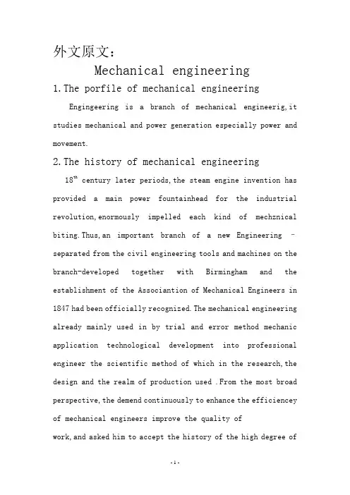
外文原文：Mechanical engineering1.The porfile of mechanical engineeringEngingeering is a branch of mechanical engineerig,it studies mechanical and power generation especially power and movement.2.The history of mechanical engineering18th century later periods,the steam engine invention has provided a main power fountainhead for the industrial revolution,enormously impelled each kind of mechznical biting.Thus,an important branch of a new Engineering –separated from the civil engineering tools and machines on the branch-developed together with Birmingham and the establishment of the Associantion of Mechanical Engineers in 1847 had been officially recognized.The mechanical engineering already mainly used in by trial and error method mechanic application technological development into professional engineer the scientific method of which in the research,the design and the realm of production used .From the most broad perspective,the demend continuously to enhance the efficienceyof mechanical engineers improve the quality of work,and asked him to accept the history of the high degree ofeducation and training.Machine operation to stress not only economic but also infrastructure costs to an absolute minimun.3.The field of mechanical engineeringThe commodity machinery development in the develop country,in the high level material life very great degree is decided each kind of which can realize in the mechanical engineering.Mechanical engineers unceasingly will invent the machine next life to produce the commodity,unceasingly will develop the accuracy and the complexity more and more high machine tools produces the machine.The main clues of the mechanical development is:In order to enhance the excellent in quality and reasonable in price produce to increase the precision as well as to reduce the production cost.This three requirements promoted the complex control system development.The most successful machine manufacture is its machine and the control system close fusion,whether such control system is essentially mechanical or electronic.The modernized car engin production transmission line(conveyer belt)is a series of complex productions craft mechanization very good example.The people are in the process of development in order to enable further automation of the production machinery ,the use of a computer to store and handle largevolumes of data,the data is a multifunctional machine tools necessary for the production of spare parts.One of the objectives is to fully automated production workshop,three rotation,but only one officer per day to operate.The development of production for mechanical machinery must have adequate power supply.Steam engine first provided the heat to generate power using practical methods in the old human,wind and hydropower,an increase of engin .New mechanical engineering industry is one of the challenges faced by the initial increase thermal effciency and power,which is as big steam turbine and the development of joint steam boilers basically achieved.20th century,turbine generators to provide impetus has been sustained and rapid growth,while thermal efficiency is steady growth,and large power plants per kW capital consumption is also declining.Finally,mechanical engineers have nuclear energy.This requires the application of nuclear energy particularly high reliability and security, which requires solving many new rge power plants and the nuclear power plant control systems have become highly complex electroonics,fluid,electricity,water and mechanical parts networks All in all areas related to the mechanical engineers.Small internal combustion engine,both to the type(petrol and diesel machines)or rotary-type(gas turbines and Mong Kerr machine),as well as their broad application in the field of transport should also due to mechanical enginerrs.Throughout the transport,both in the air and space,or in the terrestrial and marine,mechanial engineers created a variety of equipment and power devices to their increasing cooperation with electrical engineers,especially in the development of appropration control systems.Mechanical engineers in the development of military weapons technology and civil war ,needs a similar,though its purpose is to enhance rather than destroy their productivity.However.War needs a lot of resources to make the area of techonlogy,many have a far-reaching development in peacetime efficiency.Jet aircraft and nuclear reactors are well known examples.The Biological engineering,mechanical engineering biotechnology is a relatively new and different areas,it provides for the replacement of the machine or increase the body functions as well as for medical equipment.Artficial limbs have been developed and have such a strong movement and touch response function of the human body.In the development of artificial organ transplant is rapid,complex cardiac machines and similar equipment to enable increasingly complexsurgery,and injuries and ill patients life functions can be sustained.Some enviromental control mechanical engineers through the initial efforts to drainage or irrigation pumping to the land and to mine and ventilation to control the human environment.Modern refrigeration and air-conditioning plant commonaly used reverse heat engine,where the heat from the engine from cold places to more external heat.Many mechanical engineering products,as well as other leading technology development city have side effects on the environment,producing noise,water and air pollution caused,destroyed land and landscape.Improve productivity and diver too fast in the commodity,that the renewable natural forces keep pace.For mechanical engineers and others,environmental control is rapidly developing area,which includes a possible development and production of small quantities of pollutants machine sequnce,and the development of new equipment and teachnology has been to reduce and eliminate pollution.4.The role of mechanical engineeringThere are four generic mechanical engineers in common to the above all domains function.The 1st function is the understanding and the research mechanical sciencefoundation.It includes the power and movement of the relationship dynamics For example,in the vibration and movement of the relationship;Automatic control;Study of the various forms of heart,energy,power relations between the thermodynamic;Fluidflows; Heat transfer; Lubricant;And material properties.The 2nd function will be conducts the research,the desing and the development,this function in turn attempts to carry on the essential change to satisfy current and the future needs.This not only calls for a clear understanding of mechanical science,and have to break down into basic elements of a complex system capacity.But also the need for synthetic and innovative inventions.The 3rd function is produces the product and the power,include plan,operation and maintenance.Its goal lies in the maintenance either enhances the enterprise or the organization longer-tern and survivabilaty prestige at the same time,produces the greatest value by the least investments and the consumption.The 4th function is mechanical engineer’s coordinated function,including the management,the consultation,as well as carries on the market marking in certain situation.In all these function,one kind unceasingly to use thescience for a long time the method,but is not traditional or the intuition method tendency,this is a mechanical engineering skill aspect which unceasingly grows.These new rationalization means typical names include:The operations research,the engineering economics,the logical law problem analysis(is called PABLA) However,creativity is not rationalization.As in other areas,in mechanical engineering,to take unexpected and important way to bring about a new capacity,still has a personal,marked characteristice.5.The design of mechanical engineeringThe design of mechanical is the design has the mechanical property the thing or the system,such as:the instrument and the measuring appliance in very many situations,the machine design must use the knowledge of discipline the and so on mathematics,materials science and mechanics.Mechanical engineering desgin includeing all mechanical desgin,but it was a study,because it also includes all the branches of mechsnical engineering,such as thermodynamics all hydrodynamics in the basic disciplines needed,in the mechanical engineering design of the initial stude or mechanical design.Design stages.The entire desgin process from start to finish,in the process,a demand that is designed forit and decided to do the start.After a lot of repetition,the final meet this demand by the end of the design procees and the plan.Design considerations.Sometimes in a system is to decide which parts needs intensity parts of geometric shapesand size an important factor in this context that we must consider that the intensity is an important factor in the design.When we use expression design considerations,we design parts that may affect the entire system design features.In the circumstances specified in the design,usually for a series of such functions must be taken into account.Howeever,to correct purposes,we should recognize that,in many cases the design of important design considerations are not calculated or test can determine the components or systems.Especially students,wheen in need to make important decisions in the design and conduct of any operation that can not be the case,they are often confused.These are not special,they occur every day,imagine,for example,a medical laboratory in the mechanical design,from marketing perspective,people have high expectations from the strength and relevance of impression.Thick,and heavy parts installed together:to produce a solid impression machines.And sometimes machinery and spare parts from the design style is the point and not theother point of view.Our purpose is to make those you do not be misled to believe that every design decision will need reasonable mathematical methods.Manufacturing refers to the raw meterials into finished products in the enterprise.Create three distinct phases.They are:input,processing exprot.The first phase includes the production of all products in line with market needs essential.First there must be the demand for the product,the necessary materials,while also needs such as energy,time,human knowledge and technology resourcess .Finall,the need for funds to obtain all the other resources. Lose one stage after the second phase of the resources of the processes to be distributed.Processing of raw materials into finished products of these processes.To complete the design,based on the design,and then develop plans.Plan implemented through various production processes.Management of resources and processes to ensure efficiency and productivity.For example,we must carefully manage resources to ensure proper use of funds.Finally,people are talking about the product market was cast.Stage is the final stage of exporting finished or stage.Once finished just purchased,it must be delivered to the users.According to productperformance,installation and may have to conduct further debugging in addition,some products,especially those very complex products User training is necessary.6.The processes of materials and maunfacturingHere said engineering materials into two main categories:metals and non-ferrous,high-performance alloys and power metals.Non-metallic futher divided into plastice,synthetic rubber,composite materials and ceramics.It said the production proccess is divided into several major process,includingshape,forging,casting/ founding,heat treatment,fixed/connections ,measurement/ quality control and materal cutting.These processes can be further divide into each other’s craft.Various stages of the development of the manufacturing industry Over the years,the manufacturing process has four distinct stages of development, despite the overlap.These stages are:The first phase is artisanal,the second Phase is mechanization.The third phase is automation the forth Phase is integrated.When mankind initial processing of raw materials into finished products will be,they use manual processes.Each with their hands and what are the tools manuslly produced.This is totally integrated production take shape.A person needsindentification,collection materials,the design of a product to meet that demand,the production of such products and use it.From beginning to end,everything is focused on doing the work of the human ter in the industrial revolution introduced mechanized production process,people began to use machines to complete the work accomplished previously manual. This led to the specialization.Specialization in turn reduce the manufacture of integrated factors.In this stage of development,manufacturing workers can see their production as a whole represent a specific piece of the part of the production process.One can not say that their work is how to cope with the entire production process,or how they were loaded onto a production of parts finished.Development of manufacting processes is the next phase of the selection process automation.This is a computer-controlled machinery and processes.At this stage,automation island began to emerge in the workshop lane.Each island represents a clear production process or a group of processes.Although these automated isolated island within the island did raise the productivity of indivdual processes,but the overall productivity are often not change.This is because the island is not caught in other automated production process middle,but not synchronous withthem .The ultimate result is the efficient working fast parked through automated processes,but is part of the stagnation in wages down,causing bottlenecks.To better understand this problem,you can imagine the traffic in the peak driving a red light from the red Service Department to the next scene. Occasionally you will find a lot less cars,more than being slow-moving vehicles,but the results can be found by the next red light Brance.In short you real effect was to accelerate the speed of a red Department obstruction offset.If you and other drivers can change your speed and red light simultaneously.Will advance faster.Then,all cars will be consistent,sommth operation,the final everyone forward faster.In the workshop where the demand for stable synchronization of streamlined production,and promoted integration of manufacturing development.This is a still evolving technology.Fully integrated in the circumstances,is a computer-controllrd machinery and processing.integrated is completed through computer.For example in the preceding paragraph simulation problems,the computer will allow all road vehicles compatible with the change in red.So that everyone can steady traffic.Scientific analysis of movement,timing and mechanics of the disciplines is that it is composed of two pater:statics anddynamics.Statics analyzed static system that is in the system,the time is not taken into account,research and analysis over time and dynamics of the system change.Dynameics from the two componets.Euler in 1775 will be the first time two different branches: Rigid body movement studies can conveniently divided into two parts:geometric and mechanics.The first part is without taking into account the reasons for the downward movement study rigid body from a designated location to another point of the movement,and must use the formula to reflect the actual,the formula would determine the rigid body every point position. Therefore,this study only on the geometry and,more specifically,on the entities from excision.Obviously,the first part of the school and was part of a mechanical separation from the principles of dynamics to study movement,which is more than the two parts together into a lot easier.Dynamics of the two parts are subsequently divided into two separate disciplines,kinematic and dynamics,a study of movement and the movement strength.Therefore,the primary issue is the design of mechanical systems understand its kinematic.Kinematic studies movement,rather than a study of its impact.In a more precise kinematic studies position,displacement,rotation,speed,velocity and acceleration of disciplines,for esample,or planets orbiting research campaing is a paradigm.In the above quotation content should be pay attention that the content of the Euler dynamics into kinematic and rigid body dynamics is based on the assumption that they are based on research.In this very important basis to allow for the treatment of two separate disciplines.For soft body,soft body shape and even their own soft objects in the campaign depends on the role of power in their possession.In such cases,should also study the power and movement,and therefore to a large extent the analysis of the increased complexity.Fortunately, despite the real machine parts may be involved are more or less the design of machines,usually with heavy material designed to bend down to the lowest parts.Therefore,when the kinematic analysis of the performance of machines,it is often assumed that bend is negligible,spare parts are hard,but when the load is known,in the end analysis engine,re-engineering parts to confirm this assnmption.中文译文：机械工程1.机械工程简介机械工程是工程学的一个分支，它研究机械和动力的产，尤其是力和动力。