FORSTer An Efficient Heuristic for Obstacle-Avoiding Rectilinear Steiner Tree Construction

矿产资源开发利用方案编写内容要求及审查大纲
矿产资源开发利用方案编写内容要求及《矿产资源开发利用方案》审查大纲一、概述
㈠矿区位置、隶属关系和企业性质。

如为改扩建矿山, 应说明矿山现状、
特点及存在的主要问题。

㈡编制依据
(1简述项目前期工作进展情况及与有关方面对项目的意向性协议情况。

(2 列出开发利用方案编制所依据的主要基础性资料的名称。

如经储量管理部门认定的矿区地质勘探报告、选矿试验报告、加工利用试验报告、工程地质初评资料、矿区水文资料和供水资料等。

对改、扩建矿山应有生产实际资料, 如矿山总平面现状图、矿床开拓系统图、采场现状图和主要采选设备清单等。

二、矿产品需求现状和预测
㈠该矿产在国内需求情况和市场供应情况
1、矿产品现状及加工利用趋向。

2、国内近、远期的需求量及主要销向预测。

㈡产品价格分析
1、国内矿产品价格现状。

2、矿产品价格稳定性及变化趋势。

三、矿产资源概况
㈠矿区总体概况
1、矿区总体规划情况。

2、矿区矿产资源概况。

3、该设计与矿区总体开发的关系。

㈡该设计项目的资源概况
1、矿床地质及构造特征。

2、矿床开采技术条件及水文地质条件。

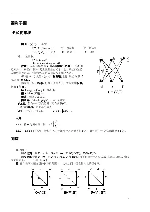
图和子图 图和简单图图 G = (V, E)， 其中 V = {νv v v ,......,,21} V ---顶点集， ν---顶点数E = {e e e 12,,......,ε}E ---边集， ε---边数例。

左图中， V={a, b,......,f}, E={p,q, ae, af,......,ce, cf} 注意， 左图仅仅是图G 的几何实现（代表）， 它们有无穷多个。

真正的 图G 是上面所给出式子，它与顶点的位置、边的形状等无关。

不过今后对两者将经常不加以区别。

称 边 ad 与顶点 a (及d) 相关联。

也称 顶点 b(及 f) 与边 bf 相关联。

称顶点a 与e 相邻。

称有公共端点的一些边彼此相邻，例如p 与af 。

环（loop ，selfloop ）：如边 l 。

棱（link ）：如边ae 。

重边：如边p 及边q 。

简单图：（simple graph ）无环，无重边 平凡图：仅有一个顶点的图（可有多条环）。

一条边的端点：它的两个顶点。

记号：νε()(),()().G V G G E G ==。

习题1.1.1 若G 为简单图，则εν≤⎛⎝ ⎫⎭⎪2 。

1.1.2 n ( ≥ 4 )个人中，若每4人中一定有一人认识其他3人，则一定有一 人认识其他n-1人。

同构在下图中， 图G 恒等于图H , 记为 G = H ⇔ V （G)=V(H), E(G)=E(H)。

图G 同构于图F ⇔ V(G)与V(F), E(G)与E(F)之间各存在一一对应关系，且这二对应关系保持关联关系。

记为 G ≅F 。

注 往往将同构慨念引伸到非标号图中，以表达两个图在结构上是否相同。

de f G = (V, E)y z w cG =(V , E )w cyz H =(V ’, E ’)’a ’c ’y ’e ’z ’F =(V ’’, E ’’)注 判定两个图是否同构是NP-hard 问题。

完全图(complete graph) Kn空图（empty g.） ⇔ E = ∅ 。

目录什么是Icepak? (2)程序结构 (2)软件功能 (3)练习一翅片散热器 (8)练习二辐射的块和板 (43)练习三瞬态分析练习四笔记本电脑练习五改进的笔记本电脑练习六 IGES模型的输入练习七非连续网格练习八 Zoom-in 建模1.1 什么是Icepak?Icepak是强大的 CAE 仿真软件工具，它能够对电子产品的传热，流动进行模拟，从而提高产品的质量，大量缩短产品的上市时间。

Icepak能够计算部件级，板级和系统级的问题。

它能够帮助工程师完成用试验不可能实现的情况，能够监控到无法测量的位置的数据。

Icepak采用的是FLUENT计算流体动力学 (CFD) 求解引擎。

该求解器能够完成灵活的网格划分，能够利用非结构化网格求解复杂几何问题。

多点离散求解算法能够加速求解时间。

Icepak提供了其它商用热分析软件不具备的特点，这些特点包括：•非矩形设备的精确模拟•接触热阻模拟•各向异性导热率•非线性风扇曲线•集中参数散热器•外部热交换器•辐射角系数的自动计算1.2 程序结构Icepak软件包包含如下内容:•Icepak, 建模，网格和后处理工具•FLUENT, 求解器图 1.2.1:软件架构Icepak本身拥有强大的建模功能。

你也可以从其它 CAD 和 CAE 软件包输入模型. Icepak 然后为你的模型做网格, 网格通过后就是进行CFD求解。

计算结果可以在Icepak中显示, 如图 1.2.1所示.1.3 软件功能所有的功能均在Icepak界面下完成。

1.3.1 总述•鼠标控制的用户界面o鼠标就能控制模型的位置，移动及改变大小o误差检查•灵活的量纲定义•几何输入IGES, STEP, IDF, 和 DXF格式•库功能•在线帮助和文档o完全的超文本在线帮助 (包括理论和练习册) •支持平台o UNIX 工作站o Windows NT 4.0/2000/XP 的PC机1.3.2 建模•基于对象的建模o cabinets 机柜o networks 网络模型o heat exchangers 热交换器o wires 线o openings 开孔o grilles 过滤网o sources 热源o printed circuit boards (PCBs) PCB板o enclosures 腔体o plates 板o walls 壁o blocks 块o fans (with hubs) 风扇o blowers 离心风机o resistances 阻尼o heat sinks 散热器o packages 封装•macros 宏o JEDEC test chambers JEDEC试验室o printed circuit board (PCB)o ducts 管道o compact models for heat sinks 简化的散热器•2D object shapes 2D模型o rectangular 矩形o circular 圆形o inclined 斜板o polygon 多边形板•complex 3D object shapes 3D模型o prisms 四面体o cylinders 圆柱o ellipsoids 椭圆柱o elliptical and concentric cylinders 椭圆柱o prisms of polygonal and varying cross-section 多面体o ducts of arbitrary cross-section 任意形状的管道1.3.3 网格•自动非结构化网格生成o六面体，四面体，五面体及混合网格•网格控制o粗网格生成o细网格生成o网格检查o非连续网格1.3.4 材料•综合的材料物性数据库•各向异性材料•属性随温度变化的材料1.3.5 物理模型•层流/湍流模型•稳态/瞬态分析•强迫对流/自然对流/混合对流•传导•流固耦合•辐射•体积阻力•混合长度方程（0-方程）, 双方程(标准- 方程), RNG - , 增强双方程 (标准- 带有增强壁面处理), 或Spalart-Allmaras 湍流模型•接触阻尼•体积阻力模型•非线性风扇曲线•集中参数的fans, resistances, and grilles1.3.6 边界条件•壁和表面边界条件：热流密度, 温度, 传热系数, 辐射,和对称边界条件•开孔和过滤网•风扇•热交换器•时间相关和温度相关的热源•随时间变化的环境温度1.3.7求解引擎对于求解器FLUENT,是采用的有限体积算法。

Optimal and Efficient Path Planning for Partially-Known EnvironmentsAnthony StentzThe Robotics Institute; Carnegie Mellon University; Pittsburgh, PA 15213AbstractThe task of planning trajectories for a mobile robot has received considerable attention in the research literature. Most of the work assumes the robot has a complete and accurate model of its environment before it begins to move; less attention has been paid to the problem of partially known environments. This situation occurs for an exploratory robot or one that must move to a goal location without the benefit of a floorplan or terrain map. Existing approaches plan an initial path based on known information and then modify the plan locally or replan the entire path as the robot discovers obstacles with its sensors, sacrificing optimality or computational efficiency respectively. This paper introduces a new algorithm, D*, capable of planning paths in unknown, partially known, and changing environments in an efficient, optimal, and complete manner.1.0IntroductionThe research literature has addressed extensively the motion planning problem for one or more robots moving through a field of obstacles to a goal. Most of this work assumes that the environment is completely known before the robot begins its traverse (see Latombe [4] for a good survey). The optimal algorithms in this literature search a state space (e.g., visibility graph, grid cells) using the dis-tance transform [2] or heuristics [8] to find the lowest cost path from the robot’s start state to the goal state. Cost can be defined to be distance travelled, energy expended, time exposed to danger, etc.Unfortunately, the robot may have partial or no information about the environment before it begins its traverse but is equipped with a sensor that is capable of measuring the environment as it moves. One approach to path planning in this scenario is to generate a “global”path using the known information and then attempt to “locally” circumvent obstacles on the route detected by the sensors [1]. If the route is completely obstructed, a new global path is planned. Lumelsky [7] initially assumes the environment to be devoid of obstacles and moves the robot directly toward the goal. If an obstacle obstructs the path, the robot moves around the perimeter until the point on the obstacle nearest the goal is found. The robot then proceeds to move directly toward the goal again. Pirzadeh [9] adopts a strategy whereby the robot wanders about the environment until it discovers the goal. The robot repeatedly moves to the adjacent location with lowest cost and increments the cost of a location each time it visits it to penalize later traverses of the same space. Korf [3] uses initial map information to estimate the cost to the goal for each state and efficiently updates it with backtracking costs as the robot moves through the environment.While these approaches are complete, they are also suboptimal in the sense that they do not generate the lowest cost path given the sensor information as it is acquired and assuming all known, a priori information is correct. It is possible to generate optimal behavior by computing an optimal path from the known map information, moving the robot along the path until either it reaches the goal or its sensors detect a discrepancy between the map and the environment, updating the map, and then replanning a new optimal path from the robot’s current location to the goal. Although this brute-force, replanning approach is optimal, it can be grossly inefficient, particularly in expansive environments where the goal is far away and little map information exists. Zelinsky [15] increases efficiency by using a quad-tree [13] to represent free and obstacle space, thus reducing the number of states to search in the planning space. For natural terrain, however, the map can encode robot traversability at each location ranging over a continuum, thus rendering quad-trees inappropriate or suboptimal.This paper presents a new algorithm for generating optimal paths for a robot operating with a sensor and a map of the environment. The map can be complete, empty, or contain partial information about the environment. ForIn Proceedings IEEE International Conference on Robotics and Automation, May 1994.regions of the environment that are unknown, the map may contain approximate information, stochastic models for occupancy, or even a heuristic estimates. The algorithm is functionally equivalent to the brute-force,optimal replanner, but it is far more efficient.The algorithm is formulated in terms of an optimal find-path problem within a directed graph, where the arcs are labelled with cost values that can range over a continuum. The robot’s sensor is able to measure arc costs in the vicinity of the robot, and the known and estimated arc values comprise the map. Thus, the algorithm can be used for any planning representation, including visibility graphs [5] and grid cell structures. The paper describes the algorithm, illustrates its operation, presents informal proofs of its soundness, optimality, and completeness, and then concludes with an empirical comparison of the algorithm to the optimal replanner.2.0The D* AlgorithmThe name of the algorithm, D*, was chosen because it resembles A* [8], except that it is dynamic in the sense that arc cost parameters can change during the problem-solving process. Provided that robot motion is properly coupled to the algorithm, D* generates optimal trajecto-ries. This section begins with the definitions and notation used in the algorithm, presents the D* algorithm, and closes with an illustration of its operation.2.1DefinitionsThe objective of a path planner is to move the robot from some location in the world to a goal location, such that it avoids all obstacles and minimizes a positive cost metric (e.g., length of the traverse). The problem space can be formulated as a set of states denoting robot loca-tions connected by directional arcs , each of which has an associated cost. The robot starts at a particular state and moves across arcs (incurring the cost of traversal) to other states until it reaches the goal state, denoted by . Every state except has a backpointer to a next state denoted by . D* uses backpointers to represent paths to the goal. The cost of traversing an arc from state to state is a positive number given by the arc cost function . If does not have an arc to , then is undefined. Two states and are neighbors in the space if or is defined.Like A*, D* maintains an list of states. The list is used to propagate information about changes to the arc cost function and to calculate path costs to states in the space. Every state has an associated tag ,such that if has never been on the list, if is currently on the list, andG X G Y b X ()Y =Y X c X Y ,()Y X c X Y ,()X Y c X Y ,()c Y X ,()OPEN OPEN X t X ()t X ()NEW =X OPEN t X ()OPEN =XOPEN if is no longer on the list. For each state , D* maintains an estimate of the sum of the arc costs from to given by the path cost function . Given the proper conditions, this estimate is equivalent to the optimal (minimal) cost from state to , given by the implicit function . For each state on the list (i.e.,), the key function,, is defined to be equal to the minimum of before modification and all values assumed by since was placed on the list. The key function classifies a state on the list into one of two types:a state if , and a state if . D* uses states on the listto propagate information about path cost increases (e.g.,due to an increased arc cost) and states to propagate information about path cost reductions (e.g.,due to a reduced arc cost or new path to the goal). The propagation takes place through the repeated removal of states from the list. Each time a state is removed from the list, it is expanded to pass cost changes to its neighbors. These neighbors are in turn placed on the list to continue the process.States on the list are sorted by their key function value. The parameter is defined to be for all such that . The parameter represents an important threshold in D*: path costs less than or equal to are optimal, and those greater than may not be optimal. The parameter is defined to be equal to prior to most recent removal of a state from the list. If no states have been removed,is undefined.An ordering of states denoted by is defined to be a sequence if for all such that and for all such that . Thus, a sequence defines a path of backpointers from to . A sequence is defined to be monotonic if( a n d) o r ( and ) for all such that . D* constructs and maintains a monotonic sequence , representing decreasing current or lower-bounded path costs, for each state that is or was on the list. Given a sequence of states , state is an ancestor of state if and a descendant of if .For all two-state functions involving the goal state, the following shorthand notation is used:.Likewise, for sequences the notation is used.The notation is used to refer to a function independent of its domain.t X ()CLOSED =X OPEN X X G h G X ,()X G o G X ,()X OPEN t X ()OPEN =k G X ,()h G X ,()h G X ,()X OPEN X OPEN RAISE k G X ,()h G X ,()<LOWER k G X ,()h G X ,()=RAISE OPEN LOWER OPEN OPEN OPEN k min min k X ()()X t X ()OPEN =k min k min k min k old k min OPEN k old X 1X N {,}b X i 1+()X i =i 1i ≤N <X i X j ≠i j (,)1i ≤j <N ≤X N X 1X 1X N {,}t X i ()CLOSED =h G X i ,()h G X i 1+,()<t X i ()OPEN =k G X i ,()h G X i 1+,()<i 1i ≤N <G X {,}X OPEN X 1X N {,}X i X j 1i j N ≤<≤X j 1j i N ≤<≤f X ()f G X ,()≡X {}G X {,}≡f °()2.2Algorithm DescriptionThe D* algorithm consists primarily of two functions: and .is used to compute optimal path costs to the goal, and is used to change the arc cost function and enter affected states on the list. Initially, is set to for all states,is set to zero, and is placed on the list. The first function,, is repeatedly called until the robot’s state,, is removed from the list (i.e.,) or a value of -1 is returned, at which point either the sequence has been computed or does not exist respectively. The robot then proceeds to follow the backpointers in the sequence until it eitherreaches the goal or discovers an error in the arc cost func-tion (e.g., due to a detected obstacle). The second function,, is immediately called to cor-rect and place affected states on the list. Let be the robot’s state at which it discovers an error in .By calling until it returns ,the cost changes are propagated to state such that . At this point, a possibly new sequence has been constructed, and the robot continues to follow the backpointers in the sequence toward the goal.T h e a l g o r i t h m s f o r a n d are presented below. The embedded routines are , which returns the state on the list with minimum value ( if the list is empty);, which returns for the list (-1 if the list is empty);, which deletes state from the list and sets ; and , w h i c h c o m p u t e s i f , if , and i f , s e t s and , and places or re-positions state on the list sorted by .In function at lines L1 through L3,the state with the lowest value is removed from the list. If is a state (i.e.,), its path cost is optimal since is equal to the old . At lines L8 through L13, each neighbor of is examined to see if its path cost can be lowered. Additionally,neighbor states that are receive an initial path cost value, and cost changes are propagated to each neighbor that has a backpointer to , regardless of whether the new cost is greater than or less than the old. Since these states are descendants of , any change to the path cost of affects their path costs as well. The backpointer of is redirected (if needed) so that the monotonic sequence is constructed. All neighbors that receive a new pathPROCESS STATE –MODIFY COST –PROCESS STATE –MODIFY COST –c °()OPEN t °()NEW h G ()G OPEN PROCESS STATE –X OPEN t X ()CLOSED =X {}X {}c °()MODIFY COST –c °()OPEN Y c °()PROCESS STATE –k min h Y ()≥Y h Y ()o Y ()=Y {}PROCESS STATE –MODIFY COST –MIN STATE –OPEN k °()NULL GET KMIN –k min OPEN DELETE X ()X OPEN t X ()CLOSED =INSERT X h new ,()k X ()h new =t X ()NEW =k X ()min k X ()h new ,()=t X ()OPEN =k X ()min h X ()h new ,()=t X ()CLOSED =h X ()h new =t X ()OPEN =X OPEN k °()PROCESS STATE –X k °()OPEN X LOWER k X ()h X ()=h X ()k min Y X NEW Y X X X Y Y {}cost are placed on the list, so that they will propagate the cost changes to their neighbors.If is a state, its path cost may not be optimal.Before propagates cost changes to its neighbors, its optimal neighbors are examined at lines L4 through L7 to see if can be reduced. At lines L15 through L18, cost changes are propagated to states and immediate descendants in the same way as for states. If is able to lower the path cost of a state that is not an immediate descendant (lines L20 and L21), is placed back on the list for future expansion. It is shown in the next section that this action is required to avoid creating a closed loop in the backpointers. If the path cost of is able to be reduced by a suboptimal neighbor (lines L23 through L25), the neighbor is placed back on the list. Thus, the update is “postponed” until the neighbor has an optimal path cost.Function: PROCESS-STATE ()L1L2if then return L3;L4if then L5for each neighbor of :L6if and then L7;L8if then L9for each neighbor of :L10if or L11( and ) or L12( and ) then L13;L14else L15for each neighbor of :L16if or L17( and ) then L18;L19else L20if and then L21L22else L23if and and L24 and then L25L26return OPEN X RAISE X h X ()NEW LOWER X X OPEN X OPEN X MIN STATE ()–=X NULL =1–k old GET KMIN –()=DELETE X ()k old h X ()<Y X h Y ()k old ≤h X ()h Y ()c Y X ,()+>b X ()Y =h X ()h Y ()c Y X ,()+=k old h X ()=Y X t Y ()NEW =b Y ()X =h Y ()h X ()c X Y ,()+≠b Y ()X ≠h Y ()h X ()c X Y ,()+>b Y ()X =INSERT Y h X ()c X Y ,()+,()Y X t Y ()NEW =b Y ()X =h Y ()h X ()c X Y ,()+≠b Y ()X =INSERT Y h X ()c X Y ,()+,()b Y ()X ≠h Y ()h X ()c X Y ,()+>INSERT X h X (),()b Y ()X ≠h X ()h Y ()c Y X ,()+>t Y ()CLOSED =h Y ()k old >INSERT Y h Y (),()GET KMIN ()–In function , the arc cost function is updated with the changed value. Since the path cost for state will change, is placed on the list. When is expanded via , it computes a new and places on the list.Additional state expansions propagate the cost to the descendants of .Function: MODIFY-COST (X, Y, cval)L1L2if then L3return 2.3Illustration of OperationThe role of and states is central to the operation of the algorithm. The states (i.e.,) propagate cost increases, and the states (i.e.,) propagate cost reductions. When the cost of traversing an arc is increased, an affected neighbor state is placed on the list, and the cost increase is propagated via states through all state sequences containing the arc. As the states come in contact with neighboring states of lower cost, these states are placed on the list, and they sub-sequently decrease the cost of previously raised states wherever possible. If the cost of traversing an arc isdecreased, the reduction is propagated via states through all state sequences containing the arc, as well as neighboring states whose cost can also be lowered.Figure 1: Backpointers Based on Initial PropagationFigure 1 through Figure 3 illustrate the operation of the algorithm for a “potential well” path planning problem.MODIFY COST –Y X OPEN X PROCESS STATE –h Y ()h X ()c X Y ,()+=Y OPEN Y c X Y ,()cval=t X ()CLOSED =INSERT X h X (),()GET KMIN ()–RAISE LOWER RAISE k X ()h X ()<LOWER k X ()h X ()=OPEN RAISE RAISE LOWER OPEN LOWER GThe planning space consists of a 50 x 50 grid of cells .Each cell represents a state and is connected to its eight neighbors via bidirectional arcs. The arc cost values are small for the cells and prohibitively large for the cells.1 The robot is point-sized and is equipped with a contact sensor. Figure 1 shows the results of an optimal path calculation from the goal to all states in the planning space. The two grey obstacles are stored in the map, but the black obstacle is not. The arrows depict the backpointer function; thus, an optimal path to the goal for any state can be obtained by tracing the arrows from the state to the goal. Note that the arrows deflect around the grey, known obstacles but pass through the black,unknown obstacle.Figure 2: LOWER States Sweep into WellThe robot starts at the center of the left wall and follows the backpointers toward the goal. When it reaches the unknown obstacle, it detects a discrepancy between the map and world, updates the map, colors the cell light grey, and enters the obstacle cell on the list.Backpointers are redirected to pull the robot up along the unknown obstacle and then back down. Figure 2illustrates the information propagation after the robot has discovered the well is sealed. The robot’s path is shown in black and the states on the list in grey.states move out of the well transmitting path cost increases. These states activate states around the1. The arc cost value of OBSTACLE must be chosen to be greater than the longest possible sequence of EMPTY cells so that a simple threshold can be used on the path cost to determine if the optimal path to the goal must pass through an obstacle.EMPTY OBSTACLE GLOWER statesRAISE statesLOWER statesOPEN OPEN RAISE LOWER“lip” of the well which sweep around the upper and lower obstacles and redirect the backpointers out of the well.Figure 3: Final Backpointer ConfigurationThis process is complete when the states reach the robot’s cell, at which point the robot moves around the lower obstacle to the goal (Figure 3). Note that after the traverse, the backpointers are only partially updated.Backpointers within the well point outward, but those in the left half of the planning space still point into the well.All states have a path to the goal, but optimal paths are computed to a limited number of states. This effect illustrates the efficiency of D*. The backpointer updates needed to guarantee an optimal path for the robot are limited to the vicinity of the obstacle.Figure 4 illustrates path planning in fractally generated terrain. The environment is 450 x 450 cells. Grey regions are fives times more difficult to traverse than white regions, and the black regions are untraversible. The black curve shows the robot’s path from the lower left corner to the upper right given a complete, a priori map of the environment. This path is referred to as omniscient optimal . Figure 5 shows path planning in the same terrain with an optimistic map (all white). The robot is equipped with a circular field of view with a 20-cell radius. The map is updated with sensor information as the robot moves and the discrepancies are entered on the list for processing by D*. Due to the lack of a priori map information, the robot drives below the large obstruction in the center and wanders into a deadend before backtracking around the last obstacle to the goal. The resultant path is roughly twice the cost of omniscientGLOWER OPEN optimal. This path is optimal, however, given the information the robot had when it acquired it.Figure 4: Path Planning with a Complete MapFigure 5: Path Planning with an Optimistic MapFigure 6 illustrates the same problem using coarse map information, created by averaging the arc costs in each square region. This map information is accurate enough to steer the robot to the correct side of the central obstruction, and the resultant path is only 6% greater incost than omniscient optimal.Figure 6: Path Planning with a Coarse-Resolution Map3.0Soundness, Optimality, andCompletenessAfter all states have been initialized to and has been entered onto the list, the function is repeatedly invoked to construct state sequences. The function is invoked to make changes to and to seed these changes on the list. D* exhibits the following properties:Property 1: If , then the sequence is constructed and is monotonic.Property 2: When the value returned by e q u a l s o r e x c e e d s , t h e n .Property 3: If a path from to exists, and the search space contains a finite number of states, will be c o n s t r u c t e d a f t e r a fi n i t e n u m b e r o f c a l l s t o . I f a p a t h d o e s n o t e x i s t , will return -1 with .Property 1 is a soundness property: once a state has been visited, a finite sequence of backpointers to the goal has been constructed. Property 2 is an optimality property.It defines the conditions under which the chain of backpointers to the goal is optimal. Property 3 is a completeness property: if a path from to exists, it will be constructed. If no path exists, it will be reported ina finite amount of time. All three properties holdX t X ()NEW =G OPEN PROCESS STATE –MODIFY COST –c °()OPEN t X ()NEW ≠X {}k min PROCESS STATE –h X ()h X ()o X ()=X G X {}PROCESS STATE –PROCESS STATE –t X ()NEW =X G regardless of the pattern of access for functions and .For brevity, the proofs for the above three properties are informal. See Stentz [14] for the detailed, formal p r o o f s. C o n s i d e r P r o p e r t y 1 fi r s t. W h e n e v e r visits a state, it assigns to point to an existing state sequence and sets to preserve monotonicity. Monotonic sequences are subsequently manipulated by modifying the functions ,,, and . When a state is placed on the list (i.e.,), is set to preserve monotonicity for states with backpointers to .Likewise, when a state is removed from the list, the values of its neighbors are increased if needed to preserve monotonicity. The backpointer of a state ,, can only be reassigned to if and if the sequence contains no states. Since contains no states, the value of every state in the sequence must be less than . Thus, cannot be an ancestor of , and a closed loop in the backpointers cannot be created.Therefore, once a state has been visited, the sequence has been constructed. Subsequent modifications ensure that a sequence still exists.Consider Property 2. Each time a state is inserted on or removed from the list, D* modifies values so that for each pair of states such that is and is . Thus, when is chosen for expansion (i.e.,), the neighbors of cannot reduce below , nor can the neighbors, since their values must be greater than . States placed on the list during the expansion of must have values greater than ; thus, increases or remains the same with each invocation of . If states with values less than or equal to are optimal, then states with values between (inclusively) and are optimal, since no states on the list can reduce their path costs. Thus, states with values less than or equal to are optimal. By induction,constructs optimal sequences to all reachable states. If the a r c c o s t i s m o d i fi e d , t h e f u n c t i o n places on the list, after which is less than or equal to . Since no state with can be affected by the modified arc cost, the property still holds.Consider Property 3. Each time a state is expanded via , it places its neighbors on the list. Thus, if the sequence exists, it will be constructed unless a state in the sequence,, is never selected for expansion. But once a state has been placedMODIFY COST –PROCESS STATE –PROCESS STATE –NEW b °()h °()t °()h °()k °()b °()X OPEN t X ()OPEN =k X ()h X ()X X h °()X b X ()Y h Y ()h X ()<Y {}RAISE Y {}RAISE h °()h Y ()X Y X X {}X {}OPEN h °()k X ()h Y ()c Y X ,()+≤X Y ,()X OPEN Y CLOSED X k min k X ()=CLOSED X h X ()k min OPEN h °()k min OPEN X k °()k X ()k min PROCESS STATE –h °()k old h °()k old k min OPEN h °()k min PROCESS STATE –c X Y ,()MODIFY COST –X OPEN k min h X ()Y h Y ()h X ()≤PROCESS STATE –NEW OPEN X {}Yon the list, its value cannot be increased.Thus, due to the monotonicity of , the state will eventually be selected for expansion.4.0Experimental ResultsD* was compared to the optimal replanner to verify its optimality and to determine its performance improve-ment. The optimal replanner initially plans a single path from the goal to the start state. The robot proceeds to fol-low the path until its sensor detects an error in the map.The robot updates the map, plans a new path from the goal to its current location, and repeats until the goal isreached. An optimistic heuristic function is used to focus the search, such that equals the “straight-line”cost of the path from to the robot’s location assuming all cells in the path are . The replanner repeatedly expands states on the list with the minimum value. Since is a lower bound on the actual cost from to the robot for all , the replanner is optimal [8].The two algorithms were compared on planning problems of varying size. Each environment was square,consisting of a start state in the center of the left wall and a goal state in center of the right wall. Each environment consisted of a mix of map obstacles (i.e., available to robot before traverse) and unknown obstacles measurable b y t h e r o b o t ’s s e n s o r. T h e s e n s o r u s e d w a s omnidirectional with a 10-cell radial field of view. Figure 7 shows an environment model with 100,000 states. The map obstacles are shown in grey and the unknown obstacles in black.Table 1 shows the results of the comparison for environments of size 1000 through 1,000,000 cells. The runtimes in CPU time for a Sun Microsystems SPARC-10processor are listed along with the speed-up factor of D*over the optimal replanner. For both algorithms, the reported runtime is the total CPU time for all replanning needed to move the robot from the start state to the goal state, after the initial path has been planned. For each environment size, the two algorithms were compared on five randomly-generated environments, and the runtimes were averaged. The speed-up factors for each environment size were computed by averaging the speed-up factors for the five trials.The runtime for each algorithm is highly dependent on the complexity of the environment, including the number,size, and placement of the obstacles, and the ratio of map to unknown obstacles. The results indicate that as the environment increases in size, the performance of D*over the optimal replanner increases rapidly. The intuitionOPEN k °()k min Y gˆX ()gˆX ()X EMPTY OPEN gˆX ()h X ()+g ˆX ()X X for this result is that D* replans locally when it detects an unknown obstacle, but the optimal replanner generates a new global trajectory. As the environment increases in size, the local trajectories remain constant in complexity,but the global trajectories increase in complexity.Figure 7: Typical Environment for Algorithm ComparisonTable 1: Comparison of D* to Optimal Replanner5.0Conclusions5.1SummaryThis paper presents D*, a provably optimal and effi-cient path planning algorithm for sensor-equipped robots.The algorithm can handle the full spectrum of a priori map information, ranging from complete and accurate map information to the absence of map information. D* is a very general algorithm and can be applied to problems in artificial intelligence other than robot motion planning. In its most general form, D* can handle any path cost opti-mization problem where the cost parameters change dur-ing the search for the solution. D* is most efficient when these changes are detected near the current starting point in the search space, which is the case with a robot equipped with an on-board sensor.Algorithm 1,00010,000100,0001,000,000Replanner 427 msec 14.45 sec 10.86 min 50.82 min D*261 msec 1.69 sec 10.93 sec 16.83 sec Speed-Up1.6710.1456.30229.30See Stentz [14] for an extensive description of related applications for D*, including planning with robot shape,field of view considerations, dead-reckoning error,changing environments, occupancy maps, potential fields,natural terrain, multiple goals, and multiple robots.5.2Future WorkFor unknown or partially-known terrains, recentresearch has addressed the exploration and map building problems [6][9][10][11][15] in addition to the path finding problem. Using a strategy of raising costs for previously visited states, D* can be extended to support exploration tasks.Quad trees have limited use in environments with cost values ranging over a continuum, unless the environment includes large regions with constant traversability costs.Future work will incorporate the quad tree representation for these environments as well as those with binary cost values (e.g., and ) in order to reduce memory requirements [15].Work is underway to integrate D* with an off-road obstacle avoidance system [12] on an outdoor mobile robot. To date, the combined system has demonstrated the ability to find the goal after driving several hundred meters in a cluttered environment with no initial map.AcknowledgmentsThis research was sponsored by ARPA, under contracts “Perception for Outdoor Navigation” (contract number DACA76-89-C-0014, monitored by the US Army TEC)and “Unmanned Ground Vehicle System” (contract num-ber DAAE07-90-C-R059, monitored by TACOM).The author thanks Alonzo Kelly and Paul Keller for graphics software and ideas for generating fractal terrain.References[1] Goto, Y ., Stentz, A., “Mobile Robot Navigation: The CMU System,” IEEE Expert, V ol. 2, No. 4, Winter, 1987.[2] Jarvis, R. A., “Collision-Free Trajectory Planning Using the Distance Transforms,” Mechanical Engineering Trans. of the Institution of Engineers, Australia, V ol. ME10, No. 3, Septem-ber, 1985.[3] Korf, R. E., “Real-Time Heuristic Search: First Results,”Proc. Sixth National Conference on Artificial Intelligence, July,1987.[4] Latombe, J.-C., “Robot Motion Planning”, Kluwer Aca-demic Publishers, 1991.[5] Lozano-Perez, T., “Spatial Planning: A Configuration Space Approach”, IEEE Transactions on Computers, V ol. C-32, No. 2,February, 1983.OBSTACLE EMPTY [6] Lumelsky, V . J., Mukhopadhyay, S., Sun, K., “Dynamic Path Planning in Sensor-Based Terrain Acquisition”, IEEE Transac-tions on Robotics and Automation, V ol. 6, No. 4, August, 1990.[7] Lumelsky, V . J., Stepanov, A. A., “Dynamic Path Planning for a Mobile Automaton with Limited Information on the Envi-ronment”, IEEE Transactions on Automatic Control, V ol. AC-31, No. 11, November, 1986.[8] Nilsson, N. J., “Principles of Artificial Intelligence”, Tioga Publishing Company, 1980.[9] Pirzadeh, A., Snyder, W., “A Unified Solution to Coverage and Search in Explored and Unexplored Terrains Using Indirect Control”, Proc. of the IEEE International Conference on Robot-ics and Automation, May, 1990.[10] Rao, N. S. V ., “An Algorithmic Framework for Navigation in Unknown Terrains”, IEEE Computer, June, 1989.[11] Rao, N.S.V ., Stoltzfus, N., Iyengar, S. S., “A ‘Retraction’Method for Learned Navigation in Unknown Terrains for a Cir-cular Robot,” IEEE Transactions on Robotics and Automation,V ol. 7, No. 5, October, 1991.[12] Rosenblatt, J. K., Langer, D., Hebert, M., “An Integrated System for Autonomous Off-Road Navigation,” Proc. of the IEEE International Conference on Robotics and Automation,May, 1994.[13] Samet, H., “An Overview of Quadtrees, Octrees andRelated Hierarchical Data Structures,” in NATO ASI Series, V ol.F40, Theoretical Foundations of Computer Graphics, Berlin:Springer-Verlag, 1988.[14] Stentz, A., “Optimal and Efficient Path Planning for Unknown and Dynamic Environments,” Carnegie MellonRobotics Institute Technical Report CMU-RI-TR-93-20, August,1993.[15] Zelinsky, A., “A Mobile Robot Exploration Algorithm”,IEEE Transactions on Robotics and Automation, V ol. 8, No. 6,December, 1992.。

FLUENT 软件操作界面中英文对照File 文件Read 读取文件：scheme 方案journal 日志 profile 外形 Write 保存文件 Import :进入另一个运算程序 Interpolate :窜改，插入Hardcopy :复制，Batch opti ons —组选项Save layout 保存设计 Grid 网格| F 屆 Grid Define Solve i-Read► Write►Import ► Export-, Interpolate —Hardcopy...Batch Options.^Save LayoutRun...RSF...ExitDefine Models模型：solver解算器Pressure based 基于压力Den sity based基于密度末解用丁 pressure based,雀改用Censity based 岀观不苻合秦相36的摄不，请甸pres 羊WE base d Al density based 慎仆则迢.41刊卜 IS 况？北外.血OC ・EHU ^ cotipled ＞（/^ ptiaw ccupl ed simple 可这孔 & pimple ijEpiso 逞划.--■轟=Sortg 冲-丸布时制* ^jfe-5-6 1844DOden ba&ed 亘工F 吋.压聲血ptessurt ba$«i 适可于那可乐册斤"dens Ply based 把丸“河悴掏t ：至殳嗟之一.刑牛可爪門d 的创R 监當歎1一，般如人锻暮叫人丄有用 轴怀，火薩墟迭牛才H5）-0 程：yje8D8-丸布门 1叫；20GS-3-7 10-2ODQ歆；I ：谢PrflSsdrfl-Bawd Soker ^Fluflnt 它星英于压力快的束解孤便丹的圮压力修止畀法"求释旳控制片悝足标联式的，擅K 家鮮不町压縮舐Mb 对于町压砂也可旦索麟；Fk«nl 6-3 tl 前的I 板』冷孵臥 B fjS4^r«^at«d &Olvar fli Cfruptod Solvtr,的实也fltje Pr#4iurft-ea5<KJ ScFvAi 约两种虽幵方ib应理拈Fluent 氐J 眇坝犢型小的.它拈垒于曲喪红旳求聲塞，最辑的出H .也桿 艮先■那式的.丰誓■載密式冇Roz AU$hk>谏方法的初和&让Fhwrt 耳有比我甘的求IT 可压胃（说 劫謹力，們耳帕榕式淮冇琴加IF 科限闾辉，倒比还丰A 完荐匚Coupted 的算送t 对子慨站何Hh 地们足便用円匕口讷油皿购 加£未处為 性上世魅端计棒低逢刈趾.擁说的DansJty-Bjiwd Solver F ft St SiMPLEC, P 怡DE 些选以的.闪为進些ffliQl ；力修止鼻袪・不金在这种类崖的我押■中氏现泊I 建址祢匹足整用Fw»ur 护P.sed Solver 堺决昧的利底*implicit 隐式， explicit 显示Space 空间：2D , axisymmetric （转动轴）， axisymmetric swirl （漩涡转动轴）；Time 时间 :steady 定常，unsteady 非定常 Velocity formulatio n 制定速度： absolute 绝对的；relative 相对的Gradient option 梯度选择：以单元作基础；以节点作基础；以单元作梯度的最小正方形。

Electric Power Systems Research 84 (2012) 58–64Contents lists available at SciVerse ScienceDirectElectric Power SystemsResearchj o u r n a l h o m e p a g e :w w w.e l s e v i e r.c o m /l o c a t e /e p srDynamic equivalence by an optimal strategyJuan M.Ramirez a ,∗,Blanca V.Hernández a ,Rosa Elvira Correa b ,1a Centro de Investigación y de Estudios Avanzados del I.P.N.,Av del Bosque 1145.Col El Bajio,Zapopan,Jal.,45019,MexicobUniversidad Nacional de Colombia –Sede Medellín.Facultad de Minas.Carrera 80#65-223Bloque M8,114,Medellín,Colombiaa r t i c l ei n f oArticle history:Received 21May 2011Received in revised form 26September 2011Accepted 29September 2011Keywords:Power system dynamics Equivalent circuitPhasor measurement unit Stability analysisPower system stabilitya b s t r a c tDue to the curse of dimensionality,dynamic equivalence remains a computational tool that helps to analyze large amount of power systems’information.In this paper,a robust dynamic equivalence is proposed to reduce the computational burden and time consuming that the transient stability studies of large power systems represent.The technique is based on a multi-objective optimal formulation solved by a genetic algorithm.A simplification of the Mexican interconnected power system is tested.An index is used to assess the proximity between simulations carried out using the full and the reduced model.Likewise,it is assumed the use of information stemming from power measurements units (PMUs),which gives certainty to such information,and gives rise to better estimates.© 2011 Elsevier B.V. All rights reserved.1.IntroductionOne way to speed up the dynamic studies of currently inter-connected power systems without significant loss of accuracy is to reduce the size of the system model by means of dynamic equiva-lents.The dynamic equivalent is a simplified dynamic model used to replace an uninterested part,known as an external part,of a power system model.This replacement aims to reduce the dimension of the original model while the part of interest remains unchanged [1–6].The phrases “Internal system”(IS)and “external system”(ES)are used in this paper to describe the area in question,and the remaining regions,respectively.Boundary buses and tie lines can be defined in each IS or ES.It is usually intended to perform detailed studies in the IS.However,the ES is important to the extent where it affects IS analyses.The equivalent does not alter the transient behavior of the part of the system that is of concern and greatly reduces the dimen-sion of the network,reducing computational time and effort [4,7,8].The dynamic equivalent also can meet the accuracy in engineering,achieving effective,rapid and precise stability analysis and security controls for large-scale power system [4,8].However,the determi-∗Corresponding author.Tel.:+523337773600.E-mail addresses:jramirez@gdl.cinvestav.mx (J.M.Ramirez),bhernande@gdl.cinvestav.mx (B.V.Hernández),elvira.correa@ (R.E.Correa).1Tel.:+57314255140.nation of dynamic equivalents may also be a time consuming task,even if performed off-line.Moreover,several dynamic equivalents may be required to represent different operating conditions of the same system.Therefore,it is important to have computational tools that automate the procedure to evaluate the dynamic equivalent [7].Ordinarily,dynamic equivalents can be constructed follow-ing two distinct approaches:(i)reduction approach,and (ii)identification approach.The reduction approach is based on an elimination/aggregation of some components of the existing model [4,5,9].The two mostly found in the literature are known as modal reduction [6,10]and coherency based aggregation [2,11,12].The identification approach is based on either parametric or non-parametric identification [13,14].In this approach,the dynamic equivalent is determined from online measurements by adjusting an assumed model until its response matches with measurements.Concerning the capability of the model,the dynamic equivalent obtained from the reduction approach is considerably more reli-able and accurate than those set up by the identification approach,because it is determined from an exact model rather than an approximation based on measurements.However,the reduction-based equivalent requires a complete set of modeling data (e.g.model,parameters,and operating status)which is rarely avail-able in practice,in particular the generators’dynamic parameters [5,13,15,16].On the other hand,due to the lack of complete system data,and/or frequently variations of the parameters with time,the importance of estimation methods is revealed noticeably.Especially,on-line model correction aids for employing adaptive0378-7796/$–see front matter © 2011 Elsevier B.V. All rights reserved.doi:10.1016/j.epsr.2011.09.023J.M.Ramirez et al./Electric Power Systems Research84 (2012) 58–6459Fig.1.190-buses46-generators power system.controllers,power system stabilizers(PSS)or transient stability assessment.The capability of such methods has become serious rival of the old conventional methods(e.g.the coherency[11,12] and the modal[6,10]approaches).The equivalent estimation meth-ods have spread,because it can be estimated founded on data measured only on the boundary nodes between the study system and the external system.This way,without any need of informa-tion from the external system,estimation process tries to estimate a reduced order linear model,which is replaced for the external part.Evidently,estimation methods can be used,in presence of perfect data of the network as well to compute the equivalent by simulation and/or model order reduction[15].Sophisticated techniques have become interesting subject for researchers to solve identification problems since90s.For example, to obtain a dynamic equivalent of an external subsystem,an opti-mization problem has been solved by the Levenberg–Marquardt algorithm[17].Artificial neural networks(ANN)are the most prevalent method between these techniques because of its high inherent ability for modeling nonlinear systems,including power system dynamic equivalents[15,18–25].Power system real time control for security and stability has pro-moted the study of on-line dynamic equivalent technologies,which progresses in two directions.One is to improve the original off-line method.The mainstream approach is to obtain equivalent model based on typical operation modes and adjust equivalent parame-ters according to real time collected information[4].Distributed coordinate calculation based on real time information exchanging makes it possible to realize on-line equivalence of multi-area inter-connected power system in power market environment[4].Ourari et al.[26]developed the slow coherency theory based on the struc-ture preservation technique,and integrated dynamic equivalence into power system simulator Hypersim,verifying the feasibility of on-line computation from both computing time and accuracy[27].Prospects of phasor measurement technique based on global positioning system(GPS)applied in transient stability control of power system are introduced in Ref.[4].Using real data collected by phasor measurement unit(PMU),with the aid of GPS and high-speed communication network,online dynamic equivalent of interconnected power grid may be achieved[4].In this paper,the dynamic equivalence problem is formulated by two objective functions.An evolutionary optimization method based on genetic algorithms is used to solve the problem.2.PropositionThe main objective of this paper is the external system’s model order reduction of an electrical grid,preserving only the frontier nodes.That is,those nodes of the external system directly linked to nodes of the study system.At such frontier nodes,fictitious gen-erators are allocated.The external boundary is defined by the user. Basically,it is composed by a set of buses,which connect the exter-nal areas to the study system.There is not restriction about this set. Different operating conditions are taken into account.work reductionAfirst condition for an equivalence strategy is the steady state preservation on the reduced grid;this means basically a precise60J.M.Ramirez et al./Electric Power Systems Research 84 (2012) 58–64Fig.2.Proposed strategy’s flowchart.voltage calculation.In this paper,all nodes of the external system are eliminated,except the frontier nodes.By a load flow study,the complex power that should inject some fictitious generators at such nodes can be calculated.The nodal balance equation yields,j ∈Jp ij +Pg i +Pl i =0,∀i ∈I(1)where I is the set of frontier nodes;J is the set of nodes linked directly to the i th frontier node;p ij is the active power flowing from the i th to j th node;Pg i is the generation at the i th node;Pl i is the load at the i th node.Thus,the voltages for the reduced model become equal to those of the full one.For studies where unbalanced conditions are important,a similar procedure could be followed for the negative and zero equivalent sequences calculation.2.2.Studied systemThe power system shown in Fig.1depicts a reduced version of the Mexican interconnected power system.It encompasses 7regional systems,with a generation capacity of 54GW in 2004and an annual consumption level of 183.3TWh in 2005.The transmis-sion grid comprises a large 400/230kV system stretching from the southern border with Central America to its northern interconnec-tions with the US.The grids at the north and south of the country are long and sparsely interconnected transmission paths.The major load centers are concentrated on large metropolitan areas,mainly Mexico City in the central system,Guadalajara City in the western system,and Monterrey City in the northeastern system.The subsystem on the right of the dotted line is considered as the system under study.Thus,the subsystem on the left is the exter-nal one.There are five frontier nodes (86,140,142,148and 188)and six frontier lines (86–184,140–141,142–143,148–143(2)and 188–187).Thus,the equivalent electrical grid has five fictitious generators at nodes 86,140,142,148and 188.Transient stabil-ity models are employed for generators,equipped with a static excitation system;its formulation is described as follows,dıdt=ω−ω0(2)dωdt=1T j [Tm −Te −D (ω−ω0)](3)dE q dt=1T d 0 −E g −(x d −x d )i d +E fd(4)dE ddt =1T d 0−E d +(x q −xq )i q (5)dE fd dt=1T A−E fd +K A (V ref +V s −|V t |) (6)where ı(rad)and ω(rad/s)represent the rotor angular positionand angular velocity;E d (pu)and E q(pu)are the internal transient voltages of the synchronous generator;E fd (pu)is the excitationvoltage;i d (pu)and i q (pu)are the d -and q -axis currents;T d 0(s)and T q 0(s)are the d -and q -open-circuit transient time constants;x’d (pu)and x q(pu)are the d -and q -transient reactances;Tm (pu)and Te (pu)are the mechanical and electromagnetic nominal torque;Tj is the moment of inertia;D is the damping factor;K A and T A (s)are the system excitation gain and time constant;V ref is the voltage reference;V t is the terminal voltage;V s is the PSS’s output (if installed).The corresponding parameters are selected as typical [28].2.3.FormulationGiven some steady state operating point (#CASES )the following objective functions are defined,min f =[f 1f 2]f 1=#CASESop =1w 1opNg intk =1ωk ori (t )−ωkequiv (x,t )2(7)f 2=#CASESop =1w 2opNg intk =1Pe kori (t )−Pe k equiv (x,t )2(8)subject to:0=Ngen eqj =1H j −ni =1i ∈LH i(9)where ωk ori is the time behavior of the angular velocity of those generators in the original system,that will be preserved (Ng int),J.M.Ramirez et al./Electric Power Systems Research84 (2012) 58–6461Fig.3.Fitness assignment of NSGA-II in the two-objective space.Fig.4.Case1:from top to bottom(i)angular position37(referred to slack);(ii)angular speed28;(iii)electrical torque41,after a three-phase fault at bus172.62J.M.Ramirez et al./Electric Power Systems Research 84 (2012) 58–64Fig.5.Case 3:from top to bottom (i)angular position 40(referred to slack);(ii)angular speed 34;(iii)electrical torque 39,after a three-phase fault at bus 144.after a disturbance within the internal area;ωk equiv is the time behavior of the angular velocity of those generators in the equiv-alent system,after the same disturbance within the internal area;Pe k ori is the time behavior of the electrical power of those gen-erators of the original system within the internal area;Pe k equiv is the time behavior of the electrical power of those generators in the equivalent system within the internal area;H k is the k th genera-tor’s inertia;L is the set of generators that belong to the external system;Ngen eq is the number of equivalent generators [16,25].The set of voltages S ={V i ,V j ,...,V k |complex voltages stemming from PMUs }has been included in the solution.The main challenge in a multi-objective optimization environ-ment is to minimize the distance of the generated solutions to the Pareto set and to maximize the diversity of the developed Pareto set.A good Pareto set may be obtained by appropriate guiding of the search process through careful design of reproduction oper-ators and fitness assignment strategies.To obtain diversification special care has to be taken in the selection process.Special care is also to be taken to prevent non-dominated solutions from being lost.Elitism addresses the problem of losing good solutions dur-ing the optimization process.In this paper,the NSGA-II algorithm (Non dominated Sorting Genetic Algorithm-II)[29–31]is used to solve the formulation.The algorithm NSGA-II has demonstrated to exhibit a well performance;it is reliable and easy to handle.It uses elitism and a crowded comparison operator that keeps diver-sity without specifying any additional parameters.Pragmatically,it is also an efficient algorithm that has shown better results to solve optimization problems with multi-objective functions in a series of benchmark problems [31,32].There are some other meth-ods that may be used.For instance,it is possible to use at least two population-based non-Pareto evolutionary algorithms (EA)and two Pareto-based EAs:the Vector Evaluated Genetic Algorithm (VEGA)[36],an EA incorporating weighted-sum aggregation [33],the Niched Pareto Genetic Algorithm [34,35],and the Nondom-inated Sorting Genetic Algorithm (NSGA)[29–31];all but VEGA use fitness sharing to maintain a population distributed along the Pareto-optimal front.3.ResultsIn this case,the decision variables,x ,are eight parametersper each equivalent generator:{x d ,x d ,x q ,x q ,T d 0,T q 0,H,D }.In this paper,for five equivalent generators,there are 40parameters to be estimated.Likewise,in this case,a random change in the load of all buses gives rise to the transient behavior.A normal distribution with zero mean is utilized to generate the increment (decrement)in all buses.The variation is limited to a maximum of 50%.The disturbance lasts for 0.12s and then it is eliminated;the studied time is 2.0s.To attain more precise equivalence for severe operating conditions,this improvement could require load variations greater than 50%.However,this bound was used in all cases.Fig.2depicts a flowchart of the followed strategy to calculate an optimal solution.In this paper,three operating points are taken into account:(i)Case 1,the nominal case [37];(ii)Case 2,an increment of 40%in load and generation;(iii)Case 3,a decrement of 30%in load and gen-eration.To account for each operating condition into the objective functions,the same weighted factors have been utilized (w i =1/3),Eqs.(7)–(8).Table 1summarizes the estimated parameters for five equiv-alent generators,according to the two objective functions.TheJ.M.Ramirez et al./Electric Power Systems Research84 (2012) 58–6463 Table1Parameters of the equivalent under a maximum of50%in load variation.G equiv1G equiv2G equiv3G equiv4G equiv5f1f2f1f2f1f2f1f2f1f2x d0.1080.104 2.140 2.100 1.920 1.9100.1590.1790.3240.362x d0.1130.1130.8190.8690.3960.3960.08760.132 1.900 1.950T d010.7010.7039.6039.6018.8018.7011.5011.5011.7011.70x q0.7100.7500.5300.5190.2880.308 2.470 2.4600.7050.803x q0.3950.3850.8740.8050.9010.9260.9220.9530.8820.884T q0 4.950 4.82033.3033.40 4.280 4.10016.9016.9012.8012.90H 4.610 4.61022.2722.2747.2647.2669.2369.2333.9333.93D18.0318.40535.6536.6239.2239.141.9042.00705.1705.2 electromechanical modes associated to generators of the internalsystem are closely preserved.These generators arefictitious andbasically are useful to preserve some of the main interarea modesbetween the internal area and the external one[16].Thus,in order to avoid the identification of the equivalent gener-ators’parameters based on a specific disturbance,in this paper theuse of random changes in all the load buses is used.This will giverise to parameters valid for different fault locations.The allowedchange in the load(in this paper,50%)will result in a slight varia-tion of transient reactances.Further studies are required to assesssensitivities.Fig.3shows a typical Pareto front for this application.The NSGA-II runs on a Matlab platform and the convergence lastsfor3.25h for a population of200individuals and20generations.It is assumed that phasor measurement units(PMUs)areinstalled at specific buses(188,140,142,148,and86in the externalsystem,and141,143,145,and182in the internal system),whichbasically correspond to the frontier nodes.Likewise,it is assumedthat the precise voltages are known in these buses every time.Bythe inclusion of the PMUs,there is a noticeable improvement in thevoltages’information at the buses near them,due to the fact that itis assumed the PMUs’high precision.In this paper,the simulation results obtained by the full andthe reduced system are compared by a closeness measure,themean squared error(MSE).The goal of a signalfidelity measureis to compare two signals by providing a quantitative score thatdescribes the degree of similarity/fidelity or,conversely,the levelof error/distortion between ually,it is assumed that oneof the signals is a pristine original,while the other is distorted orcontaminated by errors[38].Suppose that z={z i|i=1,2,...,N}and y={y i|i=1,2,...,N}aretwofinite-length,discrete signals,where N is the number of signalsamples and z i and y i are the values of the i th samples in z and y,respectively.The MSE is defined by,MSE(z,y)=1NNi=1(z i−y i)2(10)Figs.4–5illustrate the transient behavior of some representa-tive signals after a three-phase fault at buses172(Fig.4)for theCase1;and144(Fig.5)for the Case3.Bus39is selected as theslack bus.Values in Table2show the corresponding MSE valuesfor the twelve generators of the internal system for each operat-ing case.Such values indicate a close relationship between the fulland reduced signals’behavior.In order to improve the equivalenceof a specific operating point,it is possible to weight it differentlythrough the factors w1–3,Eqs.(7)–(8).Table2shows the MSE’s val-ues when Case2has a higher weighting than Case1and Case3(w2=2/3,w1=w3=1/6).These values indicate that a closer agree-ment is attained between signals with the full and the reducedmodel.It is emphasized that the equivalence’s improvement couldrequire load variations greater than50%for off-nominal operatingconditions.4.ConclusionsUndoubtedly,the power system equivalents’calculationremains a useful strategy to handle the large amount of data,cal-culations,information and time,which represent the transientstability studies of modern power grids.The proposed approachis founded on a multi-objective formulation,solved by a geneticalgorithm,where the objective functions weight independentlyeach operating condition taken into account.The use of informationstemming from PMUs helps to improve the estimated equivalentgenerators’parameters.Results indicate that the strategy is ableto closely preserve the oscillating modes associated to the inter-nal system’s generators,under different operating conditions.Thatis due to the preservation of the machines’inertia.The use ofan index to measure the proximity between the signal’s behav-ior after a three-phase fault,indicates that good agreement isattained.In this paper,the same weighting factors have been usedto assess different operating conditions into the objective func-tions.However,depending on requirements,these factors can bemodified.The equivalence based on an optimal formulation assuresTable2MSE for Case2(Three-Phase Fault at Bus168).Angular position Angular speed Electrical powerw k=1/3w2=2/3,w1=w3=1/6w k=1/3w2=2/3,w1=w3=1/6w k=1/3w2=2/3,w1=w3=1/6 Gen39 2.13E−01 1.54E−01 6.36E−05 6.90E−059.40E−02 6.91E−02Gen28 1.79E−019.39E−02 3.43E−05 2.75E−05 4.09E−05 2.50E−05Gen29 1.12E−01 4.96E−02 4.84E−05 2.29E−059.25E−04 5.38E−04Gen30 1.01E−01 4.27E−02 3.31E−05 1.62E−059.75E−04 4.52E−04Gen32 2.80E−01 1.02E−01 4.34E−05 2.69E−05 4.26E−04 5.16E−04Gen33 2.97E−01 1.09E−01 4.81E−05 3.29E−059.85E−04 1.15E−04Gen34 1.70E−01 1.04E−01 4.03E−05 4.09E−059.19E−03 6.17E−03Gen37 1.68E−01 1.08E−01 5.23E−05 5.39E−05 1.12E−028.48E−03Gen38 1.53E−019.54E−02 4.47E−05 4.60E−05 1.29E−02 1.01E−02Gen40 1.91E−01 1.15E−01 5.27E−05 5.14E−05 2.26E−03 1.06E−03Gen41 1.93E−01 1.18E−01 5.52E−05 5.39E−05 2.50E−04 1.16E−04Gen42 1.68E−01 1.07E−01 4.17E−05 4.28E−05 5.23E−05 3.02E−0564J.M.Ramirez et al./Electric Power Systems Research84 (2012) 58–64proximity between the full and the reduced models.Closer prox-imity is reached if more stringent convergence’s parameters are defined,as well as additional objective functions,as line’s power flows,are included.References[1]P.Nagendra,S.H.nee Dey,S.Paul,An innovative technique to evaluate networkequivalent for voltage stability assessment in a widespread sub-grid system, Electr.Power Energy Syst.(33)(2011)737–744.[2]A.M.Miah,Study of a coherency-based simple dynamic equivalent for transientstability assessment,IET Gener.Transm.Distrib.5(4)(2011)405–416.[3]E.J.S.Pires de Souza,Stable equivalent models with minimum phase transferfunctions in the dynamic aggregation of voltage regulators,Electr.Power Syst.Res.81(2011)599–607.[4]Z.Y.Duan Yao,Z.Buhan,L.Junfang,W.Kai,Study of coherency-based dynamicequivalent method for power system with HVDC,in:Proceedings of the2010 International Conference on Electrical and Control Engineering,2010.[5]T.Singhavilai,O.Anaya-Lara,K.L.Lo,Identification of the dynamic equiva-lent of a power system,in:44th International Universities’Power Engineering Conference,2009.[6]J.M.Undrill,A.E.Turner,Construction of power system electromechanicalequivalents by modal analysis,IEEE Trans.PAS90(1971)2049–2059.[7]A.B.Almeida,R.R.Rui,J.G.C.da Silva,A software tool for the determinationof dynamic equivalents of power systems,in:Symposium-Bulk Power System Dynamics and Control–VIII(IREP),2010.[8]A.Akhavein,M.F.Firuzabad,R.Billinton,D.Farokhzad,Review of reductiontechniques in the determination of composite system adequacy equivalents, Electr.Power Syst.Res.80(2010)1385–1393.[9]U.D.Annakkage,N.C.Nair,A.M.Gole,V.Dinavahi,T.Noda,G.Hassan,A.Monti,Dynamic system equivalents:a survey of available techniques,in:IEEE PES General Meeting,2009.[10]B.Marinescu,B.Mallem,L.Rouco,Large-scale power system dynamic equiva-lents based on standard and border synchrony,IEEE Trans.Power Syst.25(4) (2010)1873–1882.[11]R.Podmore,A.Germond,Development of dynamic equivalents for transientstability studies,Final Report on EPRI Project RP763(1977).[12]E.J.S.Pires de Souza,Identification of coherent generators considering the elec-trical proximity for drastic dynamic equivalents,Electr.Power Syst.Res.78 (2008)1169–1174.[13]P.Ju,L.Q.Ni,F.Wu,Dynamic equivalents of power systems with onlinemeasurements.Part1:theory,IEE Proc.Gener.Transm.Distrib.151(2004) 175–178.[14]W.W.Price,D.N.Ewart,E.M.Gulachenski,R.F.Silva,Dynamic equivalents fromon-line measurements,IEEE Trans.PAS94(1975)1349–1357.[15]G.H.Shakouri,R.R.Hamid,Identification of a continuous time nonlinear statespace model for the external power system dynamic equivalent by neural net-works,Electr.Power Energy Syst.31(2009)334–344.[16]J.M.Ramirez,Obtaining dynamic equivalents through the minimizationof a lineflows function,Int.J.Electr.Power Energy Syst.21(1999) 365–373.[17]J.M.Ramirez,R.Garcia-Valle,An optimal power system model order reductiontechnique,Electr.Power Energy Syst.26(2004)493–500.[18]E.de Tuglie,L.Guida,F.Torelli,D.Lucarella,M.Pozzi,G.Vimercati,Identificationof dynamic voltage–current power system equivalents through artificial neural networks,Bulk power system dynamics and control–VI,2004.[19]A.M.Azmy,I.Erlich,Identification of dynamic equivalents for distributionpower networks using recurrent ANNs,in:IEEE Power System Conference and Exposition,2004,pp.348–353.[20]P.Sowa,A.M.Azmy,I.Erlich,Dynamic equivalents for calculation of powersystem restoration,in:APE’04Wisla,2004,pp.7–9.[21]A.H.M.A.Rahim,A.J.Al-Ramadhan,Dynamic equivalent of external power sys-tem and its parameter estimation through artificial neural networks,Electr.Power Energy Syst.24(2002)113–120.[22]A.M.Stankovic, A.T.Saric,osevic,Identification of nonparametricdynamic power system equivalents with artificial neural networks,IEEE Trans.Power Syst.18(4)(2003)1478–1486.[23]A.M.Stankovic,A.T.Saric,Transient power system analysis with measurement-based gray box and hybrid dynamic equivalents,IEEE Trans.Power Syst.19(1) (2004)455–462.[24]O.Yucra Lino,Robust recurrent neural network-based dynamic equivalencingin power system,in:IEEE Power System Conference and Exposition,2004,pp.1067–1068.[25]J.M.Ramirez,V.Benitez,Dynamic equivalents by RHONN,Electr.Power Com-pon.Syst.35(2007)377–391.[26]M.L.Ourari,L.A.Dessaint,V.Q.Do,Dynamic equivalent modeling of large powersystems using structure preservation technique,IEEE Trans.Power Syst.21(3) (2006)1284–1295.[27]M.L.Ourari,L.A.Dessaint,V.Q.Do,Integration of dynamic equivalents in hyper-sim power system simulator,in:IEEE PES General Meeting,2007,pp.1–6. [28]P.M.Anderson,A.A.Fouad,Power System Control and Stability.Appendix D,The Iowa State University Press,1977.[29]K.Deb,Evolutionary algorithms for multicriterion optimization in engineer-ing design,in:Evolutionary Algorithms in Engineering and Computer Science, 1999,pp.135–161(Chapter8).[30]N.Srinivas,K.Deb,Multiple objective optimization using nondominated sort-ing in genetic algorithms,put.2(3)(1994)221–248.[31]K.Deb,A.Pratap,S.Agarwal,T.Meyarivan,A fast and elitist multi-objectivegenetic algorithm:NSGA-II,IEEE put.6(2)(2002)182–197.[32]K.Deb,Multi-Objective Optimization using Evolutionary Algorithms,1st ed.,John Wiley&Sons(ASIA),Pte Ltd.,Singapore,2001.[33]P.Hajela,C.-Y.Lin,Genetic search strategies in multicriterion optimal design,Struct.Optim.4(1992)99–107.[34]Jeffrey Horn,N.Nafpliotis,Multiobjective optimization using the niched paretogenetic algorithm,IlliGAL Report93005,Illinois Genetic Algorithms Laboratory, University of Illinois,Urbana,Champaign,July,1993.[35]J.Horn,N.Nafpliotis,D.E.Goldberg,A niched pareto genetic algorithm formultiobjective optimization,in:Proceedings of the First IEEE Conference on Evolutionary Computation,IEEE World Congress on Computational Computa-tion,vol.1,82–87,Piscataway,NJ,IEEE Service Center,1994.[36]J.D.Schafer,Multiple objective optimization with vector evaluated geneticalgorithms,in:J.J.Grefenstette(Ed.),Proceedings of an International Confer-ence on Genetic Algorithms and their Applications,1985,pp.93–100.[37]A.R.Messina,J.M.Ramirez,J.M.Canedo,An investigation on the use of powersystem stabilizers for damping inter-area oscillations in longitudinal power systems,IEEE Trans.Power Syst.13(2)(1998)552–559.[38]W.Zhou,A.C.Bovik,Mean squared error:love it or leave it?A new look at signalfidelity measures,IEEE Signal Process.Mag.26(1)(2009)98–117.。

Support vector machine:A tool for mapping mineral prospectivityRenguang Zuo a,n,Emmanuel John M.Carranza ba State Key Laboratory of Geological Processes and Mineral Resources,China University of Geosciences,Wuhan430074;Beijing100083,Chinab Department of Earth Systems Analysis,Faculty of Geo-Information Science and Earth Observation(ITC),University of Twente,Enschede,The Netherlandsa r t i c l e i n f oArticle history:Received17May2010Received in revised form3September2010Accepted25September2010Keywords:Supervised learning algorithmsKernel functionsWeights-of-evidenceTurbidite-hosted AuMeguma Terraina b s t r a c tIn this contribution,we describe an application of support vector machine(SVM),a supervised learningalgorithm,to mineral prospectivity mapping.The free R package e1071is used to construct a SVM withsigmoid kernel function to map prospectivity for Au deposits in western Meguma Terrain of Nova Scotia(Canada).The SVM classification accuracies of‘deposit’are100%,and the SVM classification accuracies ofthe‘non-deposit’are greater than85%.The SVM classifications of mineral prospectivity have5–9%lowertotal errors,13–14%higher false-positive errors and25–30%lower false-negative errors compared tothose of the WofE prediction.The prospective target areas predicted by both SVM and WofE reflect,nonetheless,controls of Au deposit occurrence in the study area by NE–SW trending anticlines andcontact zones between Goldenville and Halifax Formations.The results of the study indicate theusefulness of SVM as a tool for predictive mapping of mineral prospectivity.&2010Elsevier Ltd.All rights reserved.1.IntroductionMapping of mineral prospectivity is crucial in mineral resourcesexploration and mining.It involves integration of information fromdiverse geoscience datasets including geological data(e.g.,geologicalmap),geochemical data(e.g.,stream sediment geochemical data),geophysical data(e.g.,magnetic data)and remote sensing data(e.g.,multispectral satellite data).These sorts of data can be visualized,processed and analyzed with the support of computer and GIStechniques.Geocomputational techniques for mapping mineral pro-spectivity include weights of evidence(WofE)(Bonham-Carter et al.,1989),fuzzy WofE(Cheng and Agterberg,1999),logistic regression(Agterberg and Bonham-Carter,1999),fuzzy logic(FL)(Ping et al.,1991),evidential belief functions(EBF)(An et al.,1992;Carranza andHale,2003;Carranza et al.,2005),neural networks(NN)(Singer andKouda,1996;Porwal et al.,2003,2004),a‘wildcat’method(Carranza,2008,2010;Carranza and Hale,2002)and a hybrid method(e.g.,Porwalet al.,2006;Zuo et al.,2009).These techniques have been developed toquantify indices of occurrence of mineral deposit occurrence byintegrating multiple evidence layers.Some geocomputational techni-ques can be performed using popular software packages,such asArcWofE(a free ArcView extension)(Kemp et al.,1999),ArcSDM9.3(afree ArcGIS9.3extension)(Sawatzky et al.,2009),MI-SDM2.50(aMapInfo extension)(Avantra Geosystems,2006),GeoDAS(developedbased on MapObjects,which is an Environmental Research InstituteDevelopment Kit)(Cheng,2000).Other geocomputational techniques(e.g.,FL and NN)can be performed by using R and Matlab.Geocomputational techniques for mineral prospectivity map-ping can be categorized generally into two types–knowledge-driven and data-driven–according to the type of inferencemechanism considered(Bonham-Carter1994;Pan and Harris2000;Carranza2008).Knowledge-driven techniques,such as thosethat apply FL and EBF,are based on expert knowledge andexperience about spatial associations between mineral prospec-tivity criteria and mineral deposits of the type sought.On the otherhand,data-driven techniques,such as WofE and NN,are based onthe quantification of spatial associations between mineral pro-spectivity criteria and known occurrences of mineral deposits ofthe type sought.Additional,the mixing of knowledge-driven anddata-driven methods also is used for mapping of mineral prospec-tivity(e.g.,Porwal et al.,2006;Zuo et al.,2009).Every geocomputa-tional technique has advantages and disadvantages,and one or theother may be more appropriate for a given geologic environmentand exploration scenario(Harris et al.,2001).For example,one ofthe advantages of WofE is its simplicity,and straightforwardinterpretation of the weights(Pan and Harris,2000),but thismodel ignores the effects of possible correlations amongst inputpredictor patterns,which generally leads to biased prospectivitymaps by assuming conditional independence(Porwal et al.,2010).Comparisons between WofE and NN,NN and LR,WofE,NN and LRfor mineral prospectivity mapping can be found in Singer andKouda(1999),Harris and Pan(1999)and Harris et al.(2003),respectively.Mapping of mineral prospectivity is a classification process,because its product(i.e.,index of mineral deposit occurrence)forevery location is classified as either prospective or non-prospectiveaccording to certain combinations of weighted mineral prospec-tivity criteria.There are two types of classification techniques.Contents lists available at ScienceDirectjournal homepage:/locate/cageoComputers&Geosciences0098-3004/$-see front matter&2010Elsevier Ltd.All rights reserved.doi:10.1016/j.cageo.2010.09.014n Corresponding author.E-mail addresses:zrguang@,zrguang1981@(R.Zuo).Computers&Geosciences](]]]])]]]–]]]One type is known as supervised classification,which classifies mineral prospectivity of every location based on a training set of locations of known deposits and non-deposits and a set of evidential data layers.The other type is known as unsupervised classification, which classifies mineral prospectivity of every location based solely on feature statistics of individual evidential data layers.A support vector machine(SVM)is a model of algorithms for supervised classification(Vapnik,1995).Certain types of SVMs have been developed and applied successfully to text categorization, handwriting recognition,gene-function prediction,remote sensing classification and other studies(e.g.,Joachims1998;Huang et al.,2002;Cristianini and Scholkopf,2002;Guo et al.,2005; Kavzoglu and Colkesen,2009).An SVM performs classification by constructing an n-dimensional hyperplane in feature space that optimally separates evidential data of a predictor variable into two categories.In the parlance of SVM literature,a predictor variable is called an attribute whereas a transformed attribute that is used to define the hyperplane is called a feature.The task of choosing the most suitable representation of the target variable(e.g.,mineral prospectivity)is known as feature selection.A set of features that describes one case(i.e.,a row of predictor values)is called a feature vector.The feature vectors near the hyperplane are the support feature vectors.The goal of SVM modeling is tofind the optimal hyperplane that separates clusters of feature vectors in such a way that feature vectors representing one category of the target variable (e.g.,prospective)are on one side of the plane and feature vectors representing the other category of the target variable(e.g.,non-prospective)are on the other size of the plane.A good separation is achieved by the hyperplane that has the largest distance to the neighboring data points of both categories,since in general the larger the margin the better the generalization error of the classifier.In this paper,SVM is demonstrated as an alternative tool for integrating multiple evidential variables to map mineral prospectivity.2.Support vector machine algorithmsSupport vector machines are supervised learning algorithms, which are considered as heuristic algorithms,based on statistical learning theory(Vapnik,1995).The classical task of a SVM is binary (two-class)classification.Suppose we have a training set composed of l feature vectors x i A R n,where i(¼1,2,y,n)is the number of feature vectors in training samples.The class in which each sample is identified to belong is labeled y i,which is equal to1for one class or is equal toÀ1for the other class(i.e.y i A{À1,1})(Huang et al., 2002).If the two classes are linearly separable,then there exists a family of linear separators,also called separating hyperplanes, which satisfy the following set of equations(KavzogluandFig.1.Support vectors and optimum hyperplane for the binary case of linearly separable data sets.Table1Experimental data.yer A Layer B Layer C Layer D Target yer A Layer B Layer C Layer D Target1111112100000 2111112200000 3111112300000 4111112401000 5111112510000 6111112600000 7111112711100 8111112800000 9111012900000 10111013000000 11101113111100 12111013200000 13111013300000 14111013400000 15011013510000 16101013600000 17011013700000 18010113811100 19010112900000 20101014010000R.Zuo,E.J.M.Carranza/Computers&Geosciences](]]]])]]]–]]]2Colkesen,2009)(Fig.1):wx iþb Zþ1for y i¼þ1wx iþb rÀ1for y i¼À1ð1Þwhich is equivalent toy iðwx iþbÞZ1,i¼1,2,...,nð2ÞThe separating hyperplane can then be formalized as a decision functionfðxÞ¼sgnðwxþbÞð3Þwhere,sgn is a sign function,which is defined as follows:sgnðxÞ¼1,if x400,if x¼0À1,if x o08><>:ð4ÞThe two parameters of the separating hyperplane decision func-tion,w and b,can be obtained by solving the following optimization function:Minimize tðwÞ¼12J w J2ð5Þsubject toy Iððwx iÞþbÞZ1,i¼1,...,lð6ÞThe solution to this optimization problem is the saddle point of the Lagrange functionLðw,b,aÞ¼1J w J2ÀX li¼1a iðy iððx i wÞþbÞÀ1Þð7Þ@ @b Lðw,b,aÞ¼0@@wLðw,b,aÞ¼0ð8Þwhere a i is a Lagrange multiplier.The Lagrange function is minimized with respect to w and b and is maximized with respect to a grange multipliers a i are determined by the following optimization function:MaximizeX li¼1a iÀ12X li,j¼1a i a j y i y jðx i x jÞð9Þsubject toa i Z0,i¼1,...,l,andX li¼1a i y i¼0ð10ÞThe separating rule,based on the optimal hyperplane,is the following decision function:fðxÞ¼sgnX li¼1y i a iðxx iÞþb!ð11ÞMore details about SVM algorithms can be found in Vapnik(1995) and Tax and Duin(1999).3.Experiments with kernel functionsFor spatial geocomputational analysis of mineral exploration targets,the decision function in Eq.(3)is a kernel function.The choice of a kernel function(K)and its parameters for an SVM are crucial for obtaining good results.The kernel function can be usedTable2Errors of SVM classification using linear kernel functions.l Number ofsupportvectors Testingerror(non-deposit)(%)Testingerror(deposit)(%)Total error(%)0.2580.00.00.0180.00.00.0 1080.00.00.0 10080.00.00.0 100080.00.00.0Table3Errors of SVM classification using polynomial kernel functions when d¼3and r¼0. l Number ofsupportvectorsTestingerror(non-deposit)(%)Testingerror(deposit)(%)Total error(%)0.25120.00.00.0160.00.00.01060.00.00.010060.00.00.0 100060.00.00.0Table4Errors of SVM classification using polynomial kernel functions when l¼0.25,r¼0.d Number ofsupportvectorsTestingerror(non-deposit)(%)Testingerror(deposit)(%)Total error(%)11110.00.0 5.010290.00.00.0100230.045.022.5 1000200.090.045.0Table5Errors of SVM classification using polynomial kernel functions when l¼0.25and d¼3.r Number ofsupportvectorsTestingerror(non-deposit)(%)Testingerror(deposit)(%)Total error(%)0120.00.00.01100.00.00.01080.00.00.010080.00.00.0 100080.00.00.0Table6Errors of SVM classification using radial kernel functions.l Number ofsupportvectorsTestingerror(non-deposit)(%)Testingerror(deposit)(%)Total error(%)0.25140.00.00.01130.00.00.010130.00.00.0100130.00.00.0 1000130.00.00.0Table7Errors of SVM classification using sigmoid kernel functions when r¼0.l Number ofsupportvectorsTestingerror(non-deposit)(%)Testingerror(deposit)(%)Total error(%)0.25400.00.00.01400.035.017.510400.0 6.0 3.0100400.0 6.0 3.0 1000400.0 6.0 3.0R.Zuo,E.J.M.Carranza/Computers&Geosciences](]]]])]]]–]]]3to construct a non-linear decision boundary and to avoid expensive calculation of dot products in high-dimensional feature space.The four popular kernel functions are as follows:Linear:Kðx i,x jÞ¼l x i x j Polynomial of degree d:Kðx i,x jÞ¼ðl x i x jþrÞd,l40Radial basis functionðRBFÞ:Kðx i,x jÞ¼exp fÀl99x iÀx j992g,l40 Sigmoid:Kðx i,x jÞ¼tanhðl x i x jþrÞ,l40ð12ÞThe parameters l,r and d are referred to as kernel parameters. The parameter l serves as an inner product coefficient in the polynomial function.In the case of the RBF kernel(Eq.(12)),l determines the RBF width.In the sigmoid kernel,l serves as an inner product coefficient in the hyperbolic tangent function.The parameter r is used for kernels of polynomial and sigmoid types. The parameter d is the degree of a polynomial function.We performed some experiments to explore the performance of the parameters used in a kernel function.The dataset used in the experiments(Table1),which are derived from the study area(see below),were compiled according to the requirementfor Fig.2.Simplified geological map in western Meguma Terrain of Nova Scotia,Canada(after,Chatterjee1983;Cheng,2008).Table8Errors of SVM classification using sigmoid kernel functions when l¼0.25.r Number ofSupportVectorsTestingerror(non-deposit)(%)Testingerror(deposit)(%)Total error(%)0400.00.00.01400.00.00.010400.00.00.0100400.00.00.01000400.00.00.0R.Zuo,E.J.M.Carranza/Computers&Geosciences](]]]])]]]–]]]4classification analysis.The e1071(Dimitriadou et al.,2010),a freeware R package,was used to construct a SVM.In e1071,the default values of l,r and d are1/(number of variables),0and3,respectively.From the study area,we used40geological feature vectors of four geoscience variables and a target variable for classification of mineral prospec-tivity(Table1).The target feature vector is either the‘non-deposit’class(or0)or the‘deposit’class(or1)representing whether mineral exploration target is absent or present,respectively.For‘deposit’locations,we used the20known Au deposits.For‘non-deposit’locations,we randomly selected them according to the following four criteria(Carranza et al.,2008):(i)non-deposit locations,in contrast to deposit locations,which tend to cluster and are thus non-random, must be random so that multivariate spatial data signatures are highly non-coherent;(ii)random non-deposit locations should be distal to any deposit location,because non-deposit locations proximal to deposit locations are likely to have similar multivariate spatial data signatures as the deposit locations and thus preclude achievement of desired results;(iii)distal and random non-deposit locations must have values for all the univariate geoscience spatial data;(iv)the number of distal and random non-deposit locations must be equaltoFig.3.Evidence layers used in mapping prospectivity for Au deposits(from Cheng,2008):(a)and(b)represent optimum proximity to anticline axes(2.5km)and contacts between Goldenville and Halifax formations(4km),respectively;(c)and(d)represent,respectively,background and anomaly maps obtained via S-Afiltering of thefirst principal component of As,Cu,Pb and Zn data.R.Zuo,E.J.M.Carranza/Computers&Geosciences](]]]])]]]–]]]5the number of deposit locations.We used point pattern analysis (Diggle,1983;2003;Boots and Getis,1988)to evaluate degrees of spatial randomness of sets of non-deposit locations and tofind distance from any deposit location and corresponding probability that one deposit location is situated next to another deposit location.In the study area,we found that the farthest distance between pairs of Au deposits is71km,indicating that within that distance from any deposit location in there is100%probability of another deposit location. However,few non-deposit locations can be selected beyond71km of the individual Au deposits in the study area.Instead,we selected random non-deposit locations beyond11km from any deposit location because within this distance from any deposit location there is90% probability of another deposit location.When using a linear kernel function and varying l from0.25to 1000,the number of support vectors and the testing errors for both ‘deposit’and‘non-deposit’do not vary(Table2).In this experiment the total error of classification is0.0%,indicating that the accuracy of classification is not sensitive to the choice of l.With a polynomial kernel function,we tested different values of l, d and r as follows.If d¼3,r¼0and l is increased from0.25to1000,the number of support vectors decreases from12to6,but the testing errors for‘deposit’and‘non-deposit’remain nil(Table3).If l¼0.25, r¼0and d is increased from1to1000,the number of support vectors firstly increases from11to29,then decreases from23to20,the testing error for‘non-deposit’decreases from10.0%to0.0%,whereas the testing error for‘deposit’increases from0.0%to90%(Table4). In this experiment,the total error of classification is minimum(0.0%) when d¼10(Table4).If l¼0.25,d¼3and r is increased from 0to1000,the number of support vectors decreases from12to8,but the testing errors for‘deposit’and‘non-deposit’remain nil(Table5).When using a radial kernel function and varying l from0.25to 1000,the number of support vectors decreases from14to13,but the testing errors of‘deposit’and‘non-deposit’remain nil(Table6).With a sigmoid kernel function,we experimented with different values of l and r as follows.If r¼0and l is increased from0.25to1000, the number of support vectors is40,the testing errors for‘non-deposit’do not change,but the testing error of‘deposit’increases from 0.0%to35.0%,then decreases to6.0%(Table7).In this experiment,the total error of classification is minimum at0.0%when l¼0.25 (Table7).If l¼0.25and r is increased from0to1000,the numbers of support vectors and the testing errors of‘deposit’and‘non-deposit’do not change and the total error remains nil(Table8).The results of the experiments demonstrate that,for the datasets in the study area,a linear kernel function,a polynomial kernel function with d¼3and r¼0,or l¼0.25,r¼0and d¼10,or l¼0.25and d¼3,a radial kernel function,and a sigmoid kernel function with r¼0and l¼0.25are optimal kernel functions.That is because the testing errors for‘deposit’and‘non-deposit’are0%in the SVM classifications(Tables2–8).Nevertheless,a sigmoid kernel with l¼0.25and r¼0,compared to all the other kernel functions,is the most optimal kernel function because it uses all the input support vectors for either‘deposit’or‘non-deposit’(Table1)and the training and testing errors for‘deposit’and‘non-deposit’are0% in the SVM classification(Tables7and8).4.Prospectivity mapping in the study areaThe study area is located in western Meguma Terrain of Nova Scotia,Canada.It measures about7780km2.The host rock of Au deposits in this area consists of Cambro-Ordovician low-middle grade metamorphosed sedimentary rocks and a suite of Devonian aluminous granitoid intrusions(Sangster,1990;Ryan and Ramsay, 1997).The metamorphosed sedimentary strata of the Meguma Group are the lower sand-dominatedflysch Goldenville Formation and the upper shalyflysch Halifax Formation occurring in the central part of the study area.The igneous rocks occur mostly in the northern part of the study area(Fig.2).In this area,20turbidite-hosted Au deposits and occurrences (Ryan and Ramsay,1997)are found in the Meguma Group, especially near the contact zones between Goldenville and Halifax Formations(Chatterjee,1983).The major Au mineralization-related geological features are the contact zones between Gold-enville and Halifax Formations,NE–SW trending anticline axes and NE–SW trending shear zones(Sangster,1990;Ryan and Ramsay, 1997).This dataset has been used to test many mineral prospec-tivity mapping algorithms(e.g.,Agterberg,1989;Cheng,2008). More details about the geological settings and datasets in this area can be found in Xu and Cheng(2001).We used four evidence layers(Fig.3)derived and used by Cheng (2008)for mapping prospectivity for Au deposits in the yers A and B represent optimum proximity to anticline axes(2.5km) and optimum proximity to contacts between Goldenville and Halifax Formations(4km),yers C and D represent variations in geochemical background and anomaly,respectively, as modeled by multifractalfilter mapping of thefirst principal component of As,Cu,Pb,and Zn data.Details of how the four evidence layers were obtained can be found in Cheng(2008).4.1.Training datasetThe application of SVM requires two subsets of training loca-tions:one training subset of‘deposit’locations representing presence of mineral deposits,and a training subset of‘non-deposit’locations representing absence of mineral deposits.The value of y i is1for‘deposits’andÀ1for‘non-deposits’.For‘deposit’locations, we used the20known Au deposits(the sixth column of Table1).For ‘non-deposit’locations(last column of Table1),we obtained two ‘non-deposit’datasets(Tables9and10)according to the above-described selection criteria(Carranza et al.,2008).We combined the‘deposits’dataset with each of the two‘non-deposit’datasets to obtain two training datasets.Each training dataset commonly contains20known Au deposits but contains different20randomly selected non-deposits(Fig.4).4.2.Application of SVMBy using the software e1071,separate SVMs both with sigmoid kernel with l¼0.25and r¼0were constructed using the twoTable9The value of each evidence layer occurring in‘non-deposit’dataset1.yer A Layer B Layer C Layer D100002000031110400005000061000700008000090100 100100 110000 120000 130000 140000 150000 160100 170000 180000 190100 200000R.Zuo,E.J.M.Carranza/Computers&Geosciences](]]]])]]]–]]] 6training datasets.With training dataset1,the classification accuracies for‘non-deposits’and‘deposits’are95%and100%, respectively;With training dataset2,the classification accuracies for‘non-deposits’and‘deposits’are85%and100%,respectively.The total classification accuracies using the two training datasets are97.5%and92.5%,respectively.The patterns of the predicted prospective target areas for Au deposits(Fig.5)are defined mainly by proximity to NE–SW trending anticlines and proximity to contact zones between Goldenville and Halifax Formations.This indicates that‘geology’is better than‘geochemistry’as evidence of prospectivity for Au deposits in this area.With training dataset1,the predicted prospective target areas occupy32.6%of the study area and contain100%of the known Au deposits(Fig.5a).With training dataset2,the predicted prospec-tive target areas occupy33.3%of the study area and contain95.0% of the known Au deposits(Fig.5b).In contrast,using the same datasets,the prospective target areas predicted via WofE occupy 19.3%of study area and contain70.0%of the known Au deposits (Cheng,2008).The error matrices for two SVM classifications show that the type1(false-positive)and type2(false-negative)errors based on training dataset1(Table11)and training dataset2(Table12)are 32.6%and0%,and33.3%and5%,respectively.The total errors for two SVM classifications are16.3%and19.15%based on training datasets1and2,respectively.In contrast,the type1and type2 errors for the WofE prediction are19.3%and30%(Table13), respectively,and the total error for the WofE prediction is24.65%.The results show that the total errors of the SVM classifications are5–9%lower than the total error of the WofE prediction.The 13–14%higher false-positive errors of the SVM classifications compared to that of the WofE prediction suggest that theSVMFig.4.The locations of‘deposit’and‘non-deposit’.Table10The value of each evidence layer occurring in‘non-deposit’dataset2.yer A Layer B Layer C Layer D110102000030000411105000060110710108000091000101110111000120010131000140000150000161000171000180010190010200000R.Zuo,E.J.M.Carranza/Computers&Geosciences](]]]])]]]–]]]7classifications result in larger prospective areas that may not contain undiscovered deposits.However,the 25–30%higher false-negative error of the WofE prediction compared to those of the SVM classifications suggest that the WofE analysis results in larger non-prospective areas that may contain undiscovered deposits.Certainly,in mineral exploration the intentions are notto miss undiscovered deposits (i.e.,avoid false-negative error)and to minimize exploration cost in areas that may not really contain undiscovered deposits (i.e.,keep false-positive error as low as possible).Thus,results suggest the superiority of the SVM classi-fications over the WofE prediction.5.ConclusionsNowadays,SVMs have become a popular geocomputational tool for spatial analysis.In this paper,we used an SVM algorithm to integrate multiple variables for mineral prospectivity mapping.The results obtained by two SVM applications demonstrate that prospective target areas for Au deposits are defined mainly by proximity to NE–SW trending anticlines and to contact zones between the Goldenville and Halifax Formations.In the study area,the SVM classifications of mineral prospectivity have 5–9%lower total errors,13–14%higher false-positive errors and 25–30%lower false-negative errors compared to those of the WofE prediction.These results indicate that SVM is a potentially useful tool for integrating multiple evidence layers in mineral prospectivity mapping.Table 11Error matrix for SVM classification using training dataset 1.Known All ‘deposits’All ‘non-deposits’TotalPrediction ‘Deposit’10032.6132.6‘Non-deposit’067.467.4Total100100200Type 1(false-positive)error ¼32.6.Type 2(false-negative)error ¼0.Total error ¼16.3.Note :Values in the matrix are percentages of ‘deposit’and ‘non-deposit’locations.Table 12Error matrix for SVM classification using training dataset 2.Known All ‘deposits’All ‘non-deposits’TotalPrediction ‘Deposits’9533.3128.3‘Non-deposits’566.771.4Total100100200Type 1(false-positive)error ¼33.3.Type 2(false-negative)error ¼5.Total error ¼19.15.Note :Values in the matrix are percentages of ‘deposit’and ‘non-deposit’locations.Table 13Error matrix for WofE prediction.Known All ‘deposits’All ‘non-deposits’TotalPrediction ‘Deposit’7019.389.3‘Non-deposit’3080.7110.7Total100100200Type 1(false-positive)error ¼19.3.Type 2(false-negative)error ¼30.Total error ¼24.65.Note :Values in the matrix are percentages of ‘deposit’and ‘non-deposit’locations.Fig.5.Prospective targets area for Au deposits delineated by SVM.(a)and (b)are obtained using training dataset 1and 2,respectively.R.Zuo,E.J.M.Carranza /Computers &Geosciences ](]]]])]]]–]]]8。

第1~10题为基础题，第11~20题为提高题，第21~33为综合题注：因为在本文档中需要用到一些特殊的数学符号（如：求和号、分数等），所以当您在百度文库中浏览时，一些数学符号可能会显示不出来，不过当您把本文档下载下来在本地浏览时，所有的符号即可全部都显示出来。

^_^基础题：【1 Prime Frequency】【问题描述】给出一个仅包含字母和数字（0-9, A-Z 以及a-z）的字符串，请您计算频率（字符出现的次数），并仅报告哪些字符的频率是素数。

输入：输入的第一行给出一个整数T( 0<T<201)，表示测试用例个数。

后面的T行每行给出一个测试用例：一个字母-数字组成的字符串。

字符串的长度是小于2001的一个正整数。

输出：对输入的每个测试用例输出一行，给出一个输出序列号，然后给出在输入的字符串中频率是素数的字符。

这些字符按字母升序排列。

所谓“字母升序”意谓按ASCII 值升序排列。

如果没有字符的频率是素数，输出“empty”（没有引号）。

注：试题来源：Bangladesh National Computer Programming Contest在线测试：UV A 10789提示先离线计算出[2‥2200]的素数筛u[]。

然后每输入一个测试串，以ASCLL码为下标统计各字符的频率p[]，并按照ASCLL码递增的顺序（0≤i≤299）输出频率为素数的字符（即u [p[i]]=1且ASCLL码值为i的字符）。

若没有频率为素数的字符，则输出失败信息。

【2 Twin Primes】【问题描述】双素数（Twin Primes）是形式为(p, p+2)，术语“双素数”由Paul Stäckel (1892-1919)给出，前几个双素数是(3, 5), (5, 7), (11, 13), (17, 19), (29, 31), (41, 43)。

在本题中请你给出第S对双素数，其中S是输入中给出的整数。