Hierarchical Object-Oriented Petri Net Modeling Method based on Ontology

收稿日期:2009-04-16;修回日期:2009-06-08。

基金项目:四川省教育厅应用基础项目(08Z A029)。

作者简介:陈晓亮(1984-),男,四川成都人,硕士研究生,主要研究方向:Petri 网理论及应用;　宋文(1956-),男,四川洪雅人,教授,CCF 高级会员,主要研究方向:Petri 网理论及应用;　陈东(1983-),男,四川简阳人,硕士研究生,主要研究方向:Petri 网理论及应用。

文章编号:1001-9081(2009)10-2833-05基于Petri 网B /S 体系架构的在线评测系统建模与验证陈晓亮,宋　文,陈　东(西华大学数学与计算机学院,成都610039)(xhu_chenxl@ )摘　要:在线评测系统可以看作网络环境下,实现动态事务处理的一个有代表性的系统。

针对传统的软件设计建模方案很难兼顾系统静态结构的描述和动态行为的分析,采用P /T 网构建了一类B /S 架构的在线评测系统层次模型。

根据系统功能,提出了保证系统功能正确性应具有的重要性质,继而用S_不变量对其进行了分析、验证。

关键词:Petri 网;在线评测;B /S 架构;P /T 系统;S_不变量中图分类号:TP311 文献标志码:AM odeli n g and ver i f i ca ti on of on li n e judge system w ithB /S ba sed on Petr i netsCHE N Xiao 2liang,S ONG W en,CHEN Dong(School of M athe m atics and Co m puter Engineering,X ihua U niversity,Chengdu S ichuan 610039,China )Abstract:Online judge syste m is a rep resentative syste m in dyna m ic transacti on p r ocessing under net w ork envir on ment .The p r operties of static structure and dyna m ic behavi or were not considered by the conventi onal design method of s oft w are .A hierarchical model of online judge with B /S was constructed by P /T nets .According t o the functi on,s ome i m portant qualities were p resented t o guarantee the correctness of syste m.The analysis and verificati on of the model are shown by S_invariants .Key words:Petri net;online judge;B r owser/Server (B /S )architecture;Place /Transiti on net;S_invariant0　引言Petri 网采用可视化图形描述,但却被形式化的数学方法所支持,是一种结构化的离散事件系统(D iscrete Event Dyna m ic Syste m,DE DS )描述工具。

A transformation method of OPM Model to CPNModel for System Concept DevelopmentWenlu Zhou1,a,Feng Yang1,b,Yifan Zhu1,c1College of Information System and ManagementNational University of Defense TechnologyChangsha, Hunan,410072,Chinaa***************,b*****************,c**************.cnAbstract—Modeling languages for concept development in System Engineering usually provide a static model and lack computational capability. We introduce and implement a method combing the Object Process Methodology (OPM), a holistic modeling language well suited to describe the concept model, and Coloured Petri Net (CPN), an executable modeling language supporting elaborate simulation and analysis to make the process of System Engineering more continuous. Not only the basic entities and links, but also the hierarchical properties are converted from OPM to CPN according to the rules we proposed. Application in a simple air defense system demonstrates the process develop a concept model of OPM to a preliminary simulation model of CPN by using this method.Keywords—Object Process Methodology; Coloured Petri Nets; transformation; System EngineeringI.I NTRODUCTIONConcept development is the primary and important phase in System Engineering, since the change of it costs less and affects more. A lot of modeling languages were introduced to help understanding structures and behaviors of a system and developing a conceptual model in this phase, such as Unified Modeling Language (UML)/System Modeling Language (SysML), Object Process Methodology (OPM) and so on. Despite these languages trying to describe the dynamic behaviors of a system, they are still providing a static model and cannot fully describe the quantitative aspects. It may need simulation of the system model to explore the behaviors of the system and validate the conceptual model as well.Viewing system as a whole, OPM is more consistent with the ideal of System Engineering. It provides a holistic and hierarchical model to describe a system while UML/SysML presents different aspects of a system in separated diagrams. Although the dynamic logic of an OPM model can be checked by animation, it still cannot deal with computational behavior, which is needed in many cases.There are a lot of researches aimed at addressing this issue. S. Bolshchikov etc.[1] propose two concepts: Vivid OPM and OPM Matlab Layer, the second of which can creates Matlab code from an OPM model added a numerical computational layer and make it possible to simulate system’s behavior quantitatively. F. Simon etc.[2] suggest the possibility of combining the executable meta-language called Object-Process Network (OPN) with modeling languages including OPM. Rengzhong Wang[3] proposed a holistic modeling method for architecture development by combining the capabilities of OPM, Coloured Petri Net (CPN) and feature model. Additional information defined with CPN semantics is extended in OPM, following by mapping this model to a CPN model according rules proposed. It is a significant exploration; however, there were some shortcomings could be improved. The additional information made it more difficult for architects to build a correct OPM model and it did not mention how to convert a hierarchical OPM model to a CPN model with subnets.In this paper, a method transforming an OPM model to a CPN model by mapping OPM notations to CPN is developed and implemented. Section 2 briefly introduces the theory of OPM and CPN and points out the significance of the transformation from OPM to CPN. We introduce the transformation method in section 3, which mainly concerns the logical relationship between the different elements and procedure links in the OPM and does not need any additional information for the convert. It can also turn a hierarchical OPM model into a CPN model with subnets and keep the capability of describing complex systems of OPM to some degree. Section 4 presents an example to explain the application of the convert. Section 5 contains the conclusions and future work.II.OPM AND CPNA.Object-Process MethodologyObject-Process Methodology (OPM) is a holistic modeling language for understanding and developing systems developed by Dori [4]. It combines the object-oriented and process-oriented concepts and describes structure and behavior aspects of a system in a holistic model.Entities and links are the main building blocks of OPM. Entities include states and things (Objects and Processes). Objects are existing things, and processes are things that transform the objects by generating, consuming, or affecting them. States are situations at which the objects can exist, and belong to the objects. There are two types of links: structural links and procedural links. Structure links express the static,First International Conference on Information Science and Electronic Technology (ISET 2015)persistent relationship among objects or processes, while procedural links express the dynamics behavior of a system.OPM adopts detail decomposition rather than aspect decomposition to manage the systems’ complexity resulting in a holistic hierarchical model. OPM contains two representation modes, the graphic and textual which are semantically equivalent. Object-Process CASE tool (OPCAT) is a software environment supporting system development and lifecycle using OPM [5]B.Coloured Petri NetsColoured Petri Nets (CP-nets or CPN) is a graphical oriented language for design, specification, simulation and verification of discrete event systems [6]. It combines the capabilities of Petri nets with the programming languages and has the ability to establish a hierarchical model.The building blocks of CPN are places, transitions, tokens and arcs. Places describe the state of the system and transitions describe the actions. Arcs indicate how the state changes when the transitions occur and are presented with arc expressions. Each place contains a set of marks called tokens carrying data values which belongs to a given type corresponding to the place. The types of data values are referred as colour sets which make the tokens distinguishable from each other.CPN Tools is a mature tool supporting editing, simulation and analysis of CPN. The inscription language is Standard ML. It has different simulation modes. Monitors can be used to observe, inspect, control or modify the simulation [7]. As for analysis, CPN Tools supports state space analysis and performance analysis.C.Strengths and WeaknessesOPM and CPN have their own strengths and weaknesses. OPM is well suited to describe the concept model in system development since it provides various general semantics to describe different systems and makes them easy to understand. The view taking a system as a whole is the nature of System Engineering. However, it cannot provide enough numeric analysis which is necessary in the following assessment and validation. CPN, on the other hand, is able to support elaborate simulation and analysis especially for concurrency, however it is difficult to build a completed and correct CPN model form the very beginning. Since the two modeling languages have their own strengths in system development and neither of them can demand the needs of system design and validation alone, it is a nature thought to combine them together to complement each other. The capability of establishing a hierarchical model ensures the possibility to describe complicated systems and is crucial for the transformation.III.M ETHODAccording to the introduction above, there is a nature relationship between OPM and CPN. They both have a graphic representation. The essence of CPN is a state machine and OPM also describe the states of a system and their transformations through processes. As OPM does not have a precise mathematically definition like CPN, it is hard to give a logical representation of the covert method. One possible way is mapping the building blocks between OPM and CPN, so that models constructed by them can transform from OPM to CPN. The method is implemented by transforming the xml files.A.The Conversion of Entities and LinksThe entities in OPM are objects, processes and states. Processes are converted to transitions in CPN, since they both describe the behavior of change in a system. States are mapped to places, with the name in the format of “O_S”, where “O” stands for the name of the object the state belongs to and “S” represents the name of the state. Objects that are connected to the process without states are mapped to places. If an object connected to the process has one or more states, it does not need to be converted to a CPN place, because the procedural links will change the end to its states. Objects do not have a procedural link will not be mapped to CPN.As CPN is mainly concerned the behavior aspect of a system, structural links are not mapped to CPN. Those procedural links are divided into four types for the convert to CPN: (1) consumption links, (2) instrument links, (3) result links and (4) process links.Consumption links include consumption link and consumption event link which link from an object or a state to a process. These links are mapped to arcs from places to transitions. If the source of the link is an object with states, then build a set of arcs the sources of which are places converted from every single state of the object and add a XOR relationship among the arcs. Instead of an OR relationship, a XOR relationship fixes the number of tokens consumed in the transition. The conversion of links in following part will use a XOR relationship instead of an OR relationship as well. The XOR relationship is represented by the structure of CPN. The destinations of the set of arcs are different new transitions with the name of “P_Transition”, where “P” is the name of the source place. Then link those transitions to a new place named with the original object and then connect this new place to the transition converted from the original process as shown in the Table 1. If there is only one state of the source object, just change the source of the link to the place converted from the state.Instrument links include agent link, instrument link, effect link, instrument event link and condition link. Agent link and effect link connect an object to a process, and the rest link from an object or a state to a process. Those objects and state can trigger the process without being transformed, so the links are mapped to bidirectional arcs between places and transitions. If the source is object with states, it is similar as the consumption links except that the set of arcs are bidirectional. See Table 1.Result link which connect a process to an object or a state, are mapped to arcs from transitions to places. If the destination of the link is an object with states, then build a set of arcs the destination of which are places converted from very state of the object and the source of which is the transition converted from the process. There is a XOR relationship among the arcs which is represented by the arc expression. To build a XORrelationship, a new colour set will be declared with the name of “Xor_O”, where “O” is the name of the object. The colour set is a type of integer with the range of 0 to m-1, where m stands for the number of the states in the object. Then there will be a variable named “xor_O” which is a type of “Xor_O” and the value of it indicating a particular state. The arc expression is “if xor_O = i then 1`n else empty” where i is the number representing each states. Once the transition fires, the variable “xor_O” will be given a random value and if it equals the number representing the state, it will pass the token to the place transformed from the state, else it will pass nothing. Table 1 shows the case.Process links include invocation link and exception link, which connect two processes. A new place will be added between the two transitions converted from the processes with the name of “T1 Trigger_Event” or “T2_Exception”, where “T1” and “T2” represents the name of destination process and source process respectively. A process link is mapped to a link from the source transition to the addition place and a link from the place to the destination transition. See Table 1.TABLE I.S PECIAL CASES IN CONVERSION OF LINKSOPMCPNconsumption linkA can be s1 or s2.B consumes A .instrument linkC can be s1 or s2.D requires C .result linkF can be s1 or s2. E yields F .invocation linkG invokes H .B. The Conversion of HierarchyIn OPM, the main mechanism to manage systems’ complexity and to build a hierarchical model is in-zooming/out-zooming makes a set of lower-level things enclosed with a thing visible /invisible. There will be a new OPD for each thing that is zoomed in and the set of OPDs will be connected by the zoomed in things. In CPN, the main mechanism is substitution transitions. A substitution transition is a transition that stands for a whole page of net structure. The places related to the substitution transition are socket places. The places in subpages functioning as the interface through which subpages communicate with their parent pages are called port places. Port places are marked with an In-tag, Out-tag or I/O-tag representing an input port, output port or Input/output port respectively. Each port place of the subpageis assigned to a socket place of the substitution transition and they are functionally identical.Since in-zooming/out-zooming is prior for processes, those processes zoomed in will be mapped to substitution transition and objects zoomed in will not be mapped to CPN. The rules for turning a hierarchical OPM model to a CPN model with subnets are as follows. • A process which is zoomed in will be mapped to a substitution transition.•If the main process i.e. zoomed in process is enclosed with one or more sub-processes, the subpage will not contain the transition converted from the main process, and only presented the sub-transitions.•If the main process is not contained in the subpage, those links connected to it will be change to the sub-process. If the main process is the destination of a link which is a type of consumption links, instrument links and process links, then change the destination of the link to the first sub-process. If the main process is the source of a link, which is a type of result links and process links, then change the source of the link to the last sub-process. The order of the sub-processes is defined by their locations as the timeline in an OPD flows from the top to the bottom. The first sub-process is the one at the top and the last sub-process is the one at the bottom within the main process.•If an object appears in both parent OPD and zoomed in OPD and satisfies the condition of transforming to a place, the object in parent OPD will be a socket place and the object in zoomed in OPD will be a port place. The tag of the place is defined according to the relationship between the object and the main process. If there is only a type of consumption links, it will be an In-tag marked with the place and if there is only a type of result links, it will be an Out-tag. If there is a type of instrument links, it will be an I/O-tag. It is the same with the states within an object which appears in both parent OPD and zoomed in OPD.•The newly added places in the transformation of consumption links and process links will also considered in the conversion of hierarchy if the links appears in both parent OPD and zoomed in OPD.There are some additional rules for completing the CPN model.• The default declaration of the colour sets and variables is defined to ensure the integrity of model logic and make it possible to run. The default colour set is “INT” which is a type of integer and a default variable is “n” which is a type of “INT”. All the places are type INT and all the arc expressions are “n” which means each token carrying an integer as its data value. User-defined declarations and arc expressions can also be used to solve the specific problems. • Places without any arc from a transition to itself will have initial tokens. The default initial mark is “1`1”,which means there is one token the data value of which is one. Only one of those places transformed from a set of states in an object will have an initial token indicating the object state at the beginning. •If a process has no input which means it is not the destination of any links, there will be an additional place named “P Start”, where “P” stands for the name of the process and the place will connect to the transition converted from the process.IV. A PPLICATION IN A S IMPLE A IR D EFENSE S YSTEMFig. 1.OPD of Air Defense SystemFig. 2.OPD of the in-zoomed Detecting processFig. 3. OPD of the in-zoomed Guide&Attack processAn air defense system consists of searching radar, tracking radar, missile and command centre. Searching radar is respond for detecting the target and reporting it to the command centre, tracking radar is respond for tracking the target accurately andguiding the missile to attack the target. Missile is the weapon to attack and command centre is respond for communicating and control. We simplify the model and ignore the command centre assuming that the radars and missile can communicate well with each other. The OPM model of the simple air defense system is shown in Figure 1. The detecting process and guide and attack process can be zoomed into a new OPDand details shown in Figure 2 and Figure 3.Fig. 4.CPN of Air Defense SystemFig. 5.Subnet of the Detecting processFig. 6. Subnet of the Guide&Attack processAfter the transformation, we can get corresponding CPN shown in Figure 4, 5 and 6.It can be simulated and validated the correctness of its logic. Additional formulations and possibilities can be added into the arc expressions and the model can calculate the measurement concerned during thesimulation, like the position and speed of the target and the missile, how different possibilities of detecting affect the time of finding the target and so on.V.C ONCLUSION AND F URTHER W ORKIn this paper, we introduce and implement a method transforming an OPM model to a CPN model by mapping OPM notations to CPN. Not only the basic entities and links, but also the hierarchical properties are converted from OPM to CPN according to the rules we proposed. Combing the capabilities of describing concepts of OPM and the capabilities of simulation and analysis of CPN, it can help develop a model from concepts to details in System Engineering. Application in a simple air defense system demonstrates the process develop a concept model of OPM to a preliminary simulation model of CPN by using this method. It can make the process of concept development more continuous to some degree and make it easier to develop, analysis and validate the model.Further work based on this research might include following topics:•Transformation of the concept of time in OPM to builda timed CPN model.•Transformation based on meta-model and formulation definition of OPM and CPN.A CKNOWLEDGMENTThis research was supported by Natural Science Foundation of China (61074107,91324014).R EFERENCES[1]Bolshchikov, S., Renick, A., Somekh, J., & Dori, D. OPM Model-Driven Animated Simulation with Computational Interface to Matlab-Simulink.[2]Simona, F., Pinheiro, G., & Loureiro, G. (2007). Towards AutomaticSystems Architecting. In Complex Systems Concurrent Engineering (pp.117-130). Springer London.[3]Wang, R. (2012). Search-based system architecture development using aholistic modeling approach.[4]Dori, D. (2002). Object-Process Methodology: A Holistic SystemsParadigm; with CD-ROM (Vol. 1).[5]Dori, D., Reinhartz-Berger, I., & Sturm, A. (2003, April). OPCAT-ABimodal Case Tool for Object-Process Based System Development.In ICEIS (3) (pp. 286-291).[6]Jensen, K. (1997). A brief introduction to coloured petri nets. In Toolsand Algorithms for the Construction and Analysis of Systems (pp. 203-208). Springer Berlin Heidelberg.[7]Wells, L. (2006, October). Performance analysis using CPN tools.InProceedings of the 1st international conference on Performance evaluation methodolgies and tools (p. 59). ACM.。

基于TLA的业务流程形式化分析摘要：本文先分析了业务流程形式化分析与验证的主要研究现状，提出基于tla的业务流程形式化分析的优势。

探讨如何对tla 理论体系进行扩展，以bpel为例研究如何对主流的业务流程的描述语言进行转换。

关键词：行为时序逻辑；业务流程；形式化分析；bpel中图分类号：tp301文献标识码：a文章编号：1007-9599 (2013) 07-0000-021引言行为时序逻辑tla[1，2]是由leslielamport于1990年提出的一种基于行为逻辑与线性时态逻辑的新的逻辑方法。

通过leslielamport与一些学者的研究，compaq、microsoft公司检测工具的开发，行为时序逻辑tla，其描述语言tla+[1，2]与检测工具tlc[1，2]逐步得以完善。

本文对如何使用行为时序逻辑对电子商务环境下的业务流程进行形式化分析进行了探讨。

2业务流程形式化分析与验证的研究现状近期的研究开始关注对业务流程的规范和验证，如利用petri网、自动机、进程代数规范和验证业务服务流程的bpel模型[3，4]。

xiaochuanyi[5]利用有色petri网来设计和验证web业务服务流程，一个流程可以转换到一个对等的cp-nets模型，然后用cpn工具分析验证，检验流程的正确性。

yanpingyang[6，7]把bpel转换到层次有色网，再利用cpn工具验证。

chunouyang[8]提供了比较完整地从bpel控制流到petri网的映射。

xiangfu[9]把bpel转换成自动机，进而转换成promela语言，再利用模型验证工具spin进行验证。

wombacher等人[10]用一种扩展逻辑表达式的自动机于对业务进行形式化建模，kochutk等人[11]提出一个基于petri网的设计和验证框架，可用于bpel进程的可视化、创建和验证，文献[12]给出了一套完整的、形式化的petri网语义，将bpel进程自动转换为petri网模型，可用多种验证工具对bpel进程做自动分析。

0 型系统||type 0 system1 型系统||type 1 system2 型系统||type 2 system[返]回比矩阵||return ratio matrix[返]回差矩阵||return difference matrix[加]权函数||weighting function[加]权矩阵||weighting matrix[加]权因子||weighting factor[数字模拟]混合计算机||[digital-analog] hybrid computer[最]优化||optimizations 域||s-domainw 平面||w-planez [变换]传递函数||z-transfer functionz 变换||z-transformz 平面||z-planez 域||z-domain安全空间||safety space靶式流量变送器||target flow transmitter白箱测试法||white box testing approach白噪声||white noise伴随算子||adjoint operator伴随系统||adjoint system半实物仿真||semi-physical simulation, hardware-in-the-loop simulation 半自动化||semi-automation办公信息系统||office information system, OIS办公自动化||office automation, OA办公自动化系统||office automation system, OAS饱和特性||saturation characteristics报警器||alarm悲观值||pessimistic value背景仿真器||background simulator贝叶斯分类器||Bayes classifier贝叶斯学习||Bayesian learning备选方案||alternative被动姿态稳定||passive attitude stabilization被控变量||controlled variable; 又称“受控变量”。

doi：10.3969/j.issn.1671-1122.2020.09.006基于随机Petri网的系统安全性量化分析研究毋泽南1，田立勤1,2，陈楠2（1.青海师范大学计算机学院，西宁 810000；2.华北科技学院计算机学院，北京 101601）摘 要：针对日益频发的网络攻击事件，如何准确有效地对攻击事件进行实验推断，并对网络安全相应指标进行量化分析，已成为近年来的研究热点。

文章结合网络系统安全性评估需求，对网络系统安全性评估的主要指标及求解方法进行了论述。

在此基础上研究了利用随机Petri网对网络系统安全性进行建模分析的方法和步骤，并结合模型的马尔可夫性给出了网络系统安全性指标的计算方法。

最后，通过具体实例对模型的正确性进行验证。

结果表明，利用随机Petri网对网络系统安全性进行建模分析是合理有效的，为网络系统安全性评估相关研究提供了新思路。

关键词：网络系统安全；随机Petri网；马尔可夫性；安全评估中图分类号：TP309 文献标志码： A 文章编号：1671-1122（2020）09-0027-05中文引用格式：毋泽南，田立勤，陈楠.基于随机Petri网的系统安全性量化分析研究[J]. 信息网络安全，2020，20（9）：27-31.英文引用格式：WU Zenan, TIAN Liqin, CHEN Nan. Research on Quantitative Analysis of System Security Based on Stochastic Petri Net[J]. Netinfo Security, 2020, 20(9): 27-31.Research on Quantitative Analysis of System Security Based onStochastic Petri NetWU Zenan1, TIAN Liqin1,2, CHEN Nan2(1. School of Computer, Qinghai Normal University, Xining 810000, China;2.School of Computer, North ChinaInstitute of Science and Technology, Beijing 101601, China)Abstract: In response to the increasing frequency of network attack events, how to accurately and effectively perform experimental inference on the attack events andquantitatively analyze the corresponding indicators of network security has become a researchhotspot in recent years. This paper discusses the main indicators and solving methods ofnetwork system security assessment in conjunction with the needs of network system securityassessment. On this basis, the methods and steps of stochastic Petri nets for modeling andanalyzing network system security are studied, and the calculation method of network systemsecurity indicators is given in conjunction with the Markov property of the model. Finally, thecorrectness of the model is verified by specific examples. The results show that it is reasonableand effective to use stochastic Petri nets to model and analyze the network system security,收稿日期：2020-7-16基金项目：国家重点研发计划[2018YFC0808306]；河北省重点研发计划[19270318D]；河北省物联网监控工程技术研究中心项目[3142018055]；青海省物联网重点实验室项目[2017-ZJ-Y21]作者简介：毋泽南（1991—），男，河南，博士研究生，主要研究方向为网络实体信任评估、用户行为认证；田立勤（1970—），男，陕西，教授，博士，主要研究方向为网络安全、物联网可靠性分析；陈楠（1994—），男，安徽，硕士研究生，主要研究方向为用户行为认证。

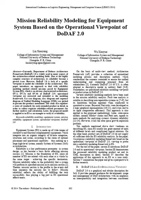
Mission Reliability Modeling for Equipment System Based on the Operational Viewpoint ofDoDAF 2.0Lin Shaoyang,College of Information System and Management National University of Defense TechnologyChangsha, P. R. China***************************Wu XiaoyueCollege of Information System and Management National University of Defense TechnologyChangsha, P. R. ChinaAbstract—Currently, Department of Defense Architecture Framework (DoDAF) 2.0 is widely used in many aspects of the architecture-related modeling fields. Due to the highly complex structure of architecture, its reliability became a pivotal issue. However, DoDAF 2.0 is lack of a specific viewpoint to model the reliability of the architecture. This paper introduces an approach to deal with reliability modeling method related missions posed by Equipment System (ES), which is an obvious characterized architecture. OV-1, OV-5a and OV-6c of DoDAF 2.0's operational viewpoint are extracted and extended as the modeling framework. Use case diagram, class diagram and sequence diagram of Unified Modeling Language (UML) are picked to present the products mentioned. The study also regulates a series of standards for each extended product in detail, in order to collect requisite reliability-related parameters for further analysis and calculation. Later, the proposed model is applied to an ES as an example to verify its availability.Keywords-reliability modeling; equipment system; mission reliability; equipment system; operational viewpoint; DoDAF2.0I.I NTRODUCTIONEquipment System (ES) is made up of wide ranges of correlative and function-complementary equipment, which integrate into an organic integrity of diverse categories, structures and scales, according to the claim of optimal placement and operational capability， thus making up a large high-level system, namely System of Systems (SoS) or architecture.Reliability is a key performance parameter in system design, so has become a basis factor affecting mission success [1]. Mission is the foundation of ES, since all member of ES are related with each other as a whole by the same target—achieving the specific destination. Mission reliability refers to the probability that a system will perform its specified mission in its mission section [2]. Therein, mission section is the profile to the events and time sequence the mission has to follow. Mission reliability reflects the ability of fulfilling the task successfully, thus playing a big part in ES operational effectiveness.On the basis of multi-view method, Architecture Framework (AF) provides a collection of normalized modeling process and description method, which standardizes the contents contained to ensure the unified understanding and comparing principal from all stakeholders [3]. Currently DoDAF 2.0 of U.S. is often adopted as descriptive model in military field [4-6]. Nonetheless, no specialized reliability modeling viewpoint or product arises in DoDAF 2.0.Several reliability modeling methods have been used in the mission reliability analysis. Fault tree analysis is suitable in describing non-repairable systems in [7–9], but its limitations become apparent when conducted to quantitative issues. Bayesian Networks were developed as a logic graphical representation [10–11], and it has shown its agile computation efficiency. This approach is also applied in the proposed methodology. Later, state-space models, namely Markov chains and Petri nets, appear as main methods for analyzing system's dynamic reliability [12-14]. However, it has the state space growth explosion problem.Yet, methods mentioned above show weakness on describing ES, since ES usually has great amount of units of different levels and complicated logical relations. On the other hand, product sets of DoDAF 2.0 do not supply all sufficient data for ES reliability analysis. In the paper, we propose a reliability modeling framework based on the operational viewpoint of DoDAF 2.0, viewing to probe into a reliability modeling framework to ES.For the rest of the paper, section II introduces DoDAF 2.0 and its operational viewpoint. Section III demonstrates the processed reliability modeling product set and its UML description in detail. Section IV describes the application of this approach to an ES as a case study. Section V summarizes the paper and gives a perspective to further research.II.D O DAF2.0A ND I TS O PERATIONAL V IEWPOINTDoDAF 2.0 is a graphical and tabular description for SoS. It provides general guidance for development, usage and management of DoD architectures with an emphasis on interoperability and integration between constituentInternational Conference on Logistics Engineering, Management and Computer Science (LEMCS 2014)systems in SoS [15]. In total, 8 viewpoints and 52 products are built in DoDAF 2.0.Viewpoint replaces "view" of antecedent versions, in order to coordinate with ISO. These viewpoints are further classified for describing the overarching aspects for every viewpoint (All Viewpoint, AV), requirements and deployments (Capability Viewpoint, CV), data relationships and alignment structure (Data and Information Viewpoint, DIV), operation scenarios and activities (Operational Viewpoint, OV), relationships between OV&CV and projects being implemented (Project Viewpoint, PV), performers, activities services and their exchanges (Service Viewpoint, SvcV), applicable principals (Standard Viewpoint, StdV), and the composition, interconnectivity and context (System Viewpoint, SV)，as Fig.1 demonstrating. Each of these views has a well-defined product set in accordance with different perspectives.The DoDAF 2.0 viewpoints reside in a presentation layer, underlying which there is a data layer where defining attributes and relationships of the architecture can be documented [16]. There is a natural and straight correspondence between AF and UML [3]. Additionally, DoDAF 2.0 formalism is increasingly being supported by other commercially available architecting tools, in which documents, sheets, matrices and such structured presentations are employed to narrow development cycle, e.g. DOORs of Telelogic, Requisite Pro of Rational and Caliber RM of Borland. One of the advantages UML possesses is that not only does it allow capturing DoDAF 2.0's data layer but also supports modeling and simulation on purpose of verification.OV describes the missions and activities, operational elements, and resource flow exchanges required to conduct operations [16]. OV is adept at tracing system's dynamic behaviors and transformation, and just such character makes it quiet suitable for modeling ES mission reliability. OV has 9 products in total, involved capturing organization relationships, resource flows, state transition and other architecture's characters. For mission reliability modeling, this paper provides a tailored product set, including OV-1, OV-5a and OV-6c to model ES's mission reliability, and it would be elaborately discussed in nextFigure 1. DoDAF 2.0 eight viewpoints.III.M ISSION R ELIABILITY M ODEL U NDER OVProduct SetThe clipped product set of ES mission reliability model is shown in Fig. 1.OV-1 aims at describing the contents and processes of the mission(s) that ES has to fulfill. Graph of jpg is recommended as the storage format. Its visualized representation enables further reliability modeling, meanwhile offering information particularly concerned by high-level decision makers during their decision process. OV-1's contents depend on the unique objective and application of specific ES. In general, it may involve operation processes, organization hierarchy, geographical distribution and operational expectations including what missions will emerge, which unit(s) will undertake, what sequences should be complied with et al, and also the interaction with external environment and systems. The links between two elements are suggested but not limited as one of the follows:∙Control: Control link from A to B means B's activity is managed by A's instructions.∙TrackInfo: TrackInfo link represents the information flow movements.∙Assistance: Assistance link from A to B indicates that if B gets failed, A would make up.∙Affirm: Affrim link reports the lower equipment's being- state and attack-complete state from lowerlevel to the command center.The relationships of the elements on the diagram sometimes convey their relative position, although this is not specifically captured in the semantics. Since each ES differs, we do not set specific rules for OV-1.OV-5a is a newly created product in DoDAF 2.0, in order to describe mission constituents and their hierarchical structure. Through the decomposition it can be cleared that the duty each mission should accomplish and unnecessary redundancy that can be eliminated. Thus the model could be simplified and efficiency may be improved as well. To clarify the affect that lower-level failure brought about to higher missions, logic connections are introduced into OV-5a. Currently 'AND' gate and 'OR' gate are mainly considered. They can be defined as follows.Def. 1AND gate: Only when all nodes under AND gate succeed does mission above the gate succeed, as Fig. 2(a).Def. 2OR gate: As long as at least one of the nodes under OR gate succeeds will mission above the gate succeed, as Fig. 2(b).OV-6c depicts the sequence and information exchanges between phases. Through constant refining to the mission process, execution order and rules would be gradually precise and accurate. UML sequence diagram is adopted as representation standard. Sequence division is consistent with divided layered graph of OV-5a. On top of the graph is ES' object, accompanied by its relevant lifeline. Specific time points are labeled on left of the lifeline labels. Bars on the lifeline stand for its duration time. Solid arrow line is message transiting between objects.In each phase's sequence diagram, time propels in terms of lifeline. In reality, lifeline is finite and does not fit for long-time phase. Thus object's lifeline should be regulated in more details. As Fig. 3 shows, on left of the object A's lifeline, t11represents A's start time and similarly t12 end time, while t21 is the time message 1 from another object arrives. t22 on the right indicates message 2 leaving time.A N DP 1P 2AO RP 1P 2BFigure 2. (a) AND gate example. (b) OR gate examplemessage 2O bj ect A t 11t12t 22message 1t 21Figure 3. OV-5a UML sequence diagram representationIV. UML D EFINITIONa. OV-5a UML normalizationOV-5a describes the operations that are normally conducted in the different nodes. The extended use-case and class diagram provides a means of breaking down activities to lower level activities as well as indicating the nodes that perform the activities. It includes node, activity, link and logic relation. Their normalized data definition is shown in table 2 (a)-(d).b. OV-5a UML normalizationThe OV-6c is used to define time based behavioral scenarios between operational elements. The interactions can be service operations as well as the interactions defined on OV-5a diagrams. There are three types of elements in OV-6c: node, lifeline and message transit. Therein, node data definition is the same as OV-5a. Lifeline can be potentially described by the messageArrivingTime and messageLeavingTime attributes of message transit. Table 3 illustrates the data definition for message transit.TABLE I.ES M ISSION R ELIABILITY M ODELTABLE II.(A)D ATA D EFINITION F OR N ODETABLE III. (A) D ATA D EFINITION M ESSAGE TRANSITV.C ASE S TUDYAn ES is presented in this part as a detailed illustration to the proposed model. The system basically consists of five parts: Ground Based Interceptor (GBI), X band Ground Based Rader (GBR), Battle Management and Command, Control & Communications (BM/C3) system, Upgraded Early Warning Radar (UEWR), and Defense Support Program/Space-Based Infrared System (DSP/SBIRS) [17].GBI is an up-to-date kinetic energy antipersonnel weapon intercepting ballistic missile warheads in its midcourse outside the atmosphere and destroying it through straightly impact. Traditional GBI consists of Exoatmospheric Kill Vehicle (EKV) and two booster rockets.GBR is X band phased array radar, and it is the main fire control radar of the system, deployed at the same place with GBI. It mainly involves surveillance, capture, trace, identification, fire control assistance and damage evaluation.BM/C3 is the brain of system, connecting all constituent systems organically. It mainly involves in receiving data from each detector to analyze the striking missile's parameters (like speed, trajectory, point of fall et. al), calculating "sweet point", directing UEWR and GBR to trace and capture the target, giving launch orders to GBI, offering revised target information to the flying interceptor, evaluation intercepting effect, and so on. BM/C3 is also deployed with GBI and GBR.UWER is upgraded phased array radar used to detect and track ballistic missile and provide early warnings. It detects and traces ballistic missile initial flight and provides GBR rough azimuth information.DSP supplies early warnings for the system. Via merging data from two or more DSPs, ballistic trajectory can be forecasted. Furthermore, compared with foregone missiles' infrared characteristics, the ballistic version can be confirmed. Currently, DSP is gradually replaced by SBIRS, which consists of two kinds satellites: Lower Earth Orbit (LEO) and High Earth Orbit (HEO). Highly flexible infrared sensor technique of HEO conveys strategy, the launch and flight of theatre ballistic missile, global theatre infrared data and processed intelligence. LEO satellites are equipped with two kind sensors: the capture one is to observe flame during the rocket launch phase; the other trace one could keep in track with the locked target from its midcourse until back into the atmosphere.Fig. 4 is the OV-1 model of the system. Substantially the system functions in such procedures:1: Early warning phase1) DSP/SBIRS detects the booster's plume when the striking ballistic missiles launches, and traces until its booster rocker turning off. Via repeater satellite or earth station, DSP/SBIRS sends trackinfo back to BM/C3for predicting the striking missile's incoming direction as well as impact area. Pertinent data would also be sent to UEWR.2) After gets information of ballistic position, UEWR will search and detect associative airspace to trace the striking missile. When discovering missile warhead, it will track robustly and send trackinfo to BM/C3.2: Interception decision phase1) BM/C3formulates operations management plan, including intercepting pattern, interceptor quantity, calculating effective acting distance, thus preliminarily ascertaining GBI's launch direction and moment. Meanwhile BM/C3should send control information to GBI and receive affirm to get its authorization.2) BM/C3 sends trackinfo got from UEWR to GBR to guide its search. Through detecting and tracing ballistic warhead, GBR would retrieve more precise information for BM/C3decision. Meanwhile, GBR would generate warhead image by sufficient data it has collected.3) BM/C3conducts target identification and threat evaluation to verify the warhead version, the trajectory and the impact point. On this basis, interception decision about GBI's launch moment and estimated interception point is made. When the accuracy of the estimated interception point is within the appointed scope (20km), BM/C3 would give GBI launching orders targeting on the estimated interception point.3：Interception implementation phase1) As soon as receiving orders, GBI launches immediately. After that, GBR precisely tracks GBI and warhead, returns revised objective data back to BM/C3 to update GBI's flight.2) When GBI reaches the estimated airspace, EKV separates with the booster rocket. Then EKV compares the target information detected with former images provided by GBR to verify and target objective, thus destroying it through straight collision.4： Interception effectiveness evaluation1) During the GBI collision, GBR collects interception data sending back to BM/C3.2) BM/C3evaluated the interception effectiveness. If failed, BM/C3 has to decide whether to conduct a second interception.According to the procedure, its operational activities decomposition can be depicted like Fig. 5(a). Furthermore, Fig. 5(b) shows the class diagram for the case "EKV attack". On purpose of saving space, some of the class attribute values and operations have been omitted. For the proposed model of OV-6c, the above mentioned interception decision phase is hired as an example, and it is shown in Fig. 6.VI.C ONCLUSIONDoDAF 2.0 is a rife model framework for ES. The paper proposes a mission reliability modeling method based on the operational viewpoint of DoDAF 2.0 and illustrates the UML normalization. An ES is an example of highly complex and adaptive ES characterized by a loosely coupled federation of constituent systems. The proposed model succeeds in describing ES reliability structure, proving the methods validity. For further research, transition mechanism between OV-5a and OV-5b can be investigated in terms of enriching the product set and heterogeneous representation. Besides, UML entities can be enlarged for more abundant and convenient details. More importantly, system view's product can also be used on mission reliability modeling.A CKNOWLEDGMENTThe paper is partly supported by National Natural Science Foundation of China under grant no. 71071159.Figure 4.OV-1 modelD S P /S B I R Sdet ect pl um et racem i ssi l est ore dat asend i nf o.recei ve com m andU E W Rsearchw arheadG B IG B Rl aunch gi ve orders<extends><extends>revi se fli ghtseparat eboost ersE K V at t ack<extends><extends><extends>recei vei nf o.cal cul at edeci degenerat ei m ageFigure 5. (a) OV-5a modelactivityIDnodeContained activityDescription successrulesE K VA t t acknodeId ofActivity linkIn linkToprerequisitesuccessProbability startTime endTimeE K V S eparat enodeId ofActivity linkIn linkToprerequisitesuccessProbability startTime endTimeA t t ackO rdermessageType messageIdmessageFrom: GBR, UEWR messageArrivingTime Fl i ght P osi t i onE K V posi t i oni ngmessageType messageIdmessageFrom: GBR messageArrivingTimeR evi sed Fl i ght ANDmessageType messageId messageFrom messageTomessageArrivingTime messageLeavingTimeTarget V eri ficat i on ANDFigure 5. (b) OV-5a class diagram for the case "EKV attack"U E W RG B RB M /C 31: controlAuthorizationG B I6: launch decision order(position,time)3: traceMessage5: traceMessagewarhead image4: traceMessage 2: af f i r m at i onFigure 6. OV-6c Sequence diagram for interception decision phaseR EFERENCES[1] Reliability primer for command, control, communications,computer, intelligence, surveillance, and reconnaisssance (C4ISR) facilities. available at: http: // www. usace. ary. mil /publications/ armytm/tm5-698-3/entire.pdf.2005a.[2] Chul Kim, “Analysis for mission reliability of a combat tank ,”IEEE Transactions on Reliability, vol. 38, no. 2, pp 242-245, 1989. [3] Robert K. Garrett, Steve A., Neil T Baron, “Managing theinterstitials, a system of systems framework suited for the ballistic missile defense system ,” Systems Engineering, vol 14,no. 1, pp. 87-108,2011.[4] Yang Kewei and Tan Yuejin, Architecture RequirementsTechnique and Method. Peking: Science Press, 2010.[5] Shu Yu, Research on weapon equipment architecture modelingmethod and application based on the capability requirements, Ph.D. Dissertation, National University of Defense Technology, 2009. [6] Jiang Zhiping, Research on architecture verification method andkey technique for C4ISR system based on CADM, Ph.D. Dissertation, National University of Defense Technology, 2007. [7] Bobbio A., Portinale L, “Improving the analysis of dependablesystems by mapping fault trees into Bayesian networks ,” Reliability Engineering & System Safety, vol. 71, no. 5, pp 249-260, 2001.[8] Hichem Boudali, Joanne,Bechta Dugan, “Dynamic fault treemodels for fault tolerant computer systems ,” IEEE Transaction On Reliability, vol. 41, no. 3, pp 363-377, 1992.[9] Huang Chin-Yu, Chang Yung-Ruei, “An improved decompositionscheme for assessing the reliability of embedded systems by using dynamic fault trees,” Reliability Engineering & System Safety, vol 92, no. 10, pp 1403-1412, 2007.[10] Boudali H., Dugan J. B, “A discrete-time Bayesian networkreliability modeling and analysis framework ,” Reliability Engineering & System Safety, vol 87, no. 6, pp 337-349, 2005. [11] Hichem Boudali, Joanne Bechta Dugan, “A continuous-timeBayesian network reliability modeling and analysis framework ,” IEEE Transaction On Reliability, vol 55, no. 1, pp 34-41, 2006. [12] Jau-Yeu Menq, Pan-Chio Tuan, “Discrete Markov ballistic missiledefense system modeling ,” European Journal of Operational Research, vol 178, no. 1, pp 560-578, 2007.[13] Kim K, Park S, “Phased-mission system reliability under Markovenvironment ,” IEEE Transaction On Reliability, vol 43, no. 5, pp 301-309, 1994.[14] Abidin E.Olmez, “Mission centric reliability analysis of C4ISRarchitectures using petri net ,” In Proceedings of IEEE International Conference on Systems, Man and Cybernetics, pp 587-592, 2003. [15] Department of Defense Architecture Working Group, DoDArchitecture Framework 2.0, Volume 2: Architecture and Models, available at: /Portals/0/Documents/DODAF/DoDAF_v2-02_web.pdf[16] Biswas, A, Hayden, J, Phillips, MS, Bhasin, KB, Putt, C, &Sartwell, T, “Applying DoDAF to NASA orion mission communication and navigation architecture. In Proceedings of IEEE Aerospace Conference, pp 1-9, 2008.[17] Wang Minle and Li Yong, Ballistic Missile PenetrationEffectiveness Analysis. Peking: National Defense Industry Press, 2010.。

Winfrid G. SchneeweissPetri Nets for Reliability Modeling(in the Fields of EngineeringSafety and Dependability)LiLoLe-Verlag GmbH (Publ.Co.Ltd.)Serving Life-Long LearningPrologThis book of LiLoLe-V erlag (=publisher) was prepared with life-long learning in mind. This means easy reading as tol the level of presentation ( tutorial, rather than research type)l the didactics of explanationsl complete solutions of all the exercises(important for self-study)l the quality and number of the figuresl the text layoutl the size of the letters (still legible in case of deteriorated sight)l the size of the book ( useful as a little intellectual refresher that can be mastered during a single week)Here comes a book to be read for earnest study and professional use, or just for fun at any age from, say, 17.Table of contentsPreface1 Introduction1.1The main aim of this book1.2A preliminary description of Petri nets1.3How to work with this book2Basics of Petri nets2.1Definition of Petri nets2.2State graphs of Petri nets (reachability graphs)2.3A chess board pattern for drawing Petri nets2.4Modeling basic switching phenomena2.5Inhibit edges2.6Exercises3Special aspects of Petri nets with reliability modeling 3.1Petri nets of state graphs3.2Petri nets of fault trees and success trees3.3The different meanings of tokens3.4Exercises4Non-repairable systems4.1Systems without redundancy4.2Systems with cold standby4.3Systems with hot standby4.4Exercises5Repairable systems I; basic aspects5.1Repair after a diagnosis process5.2Repair priorities; simple cases5.3Toward a systematic design of modules5.4Integrating fault tree and success tree5.5Exercises6Repairable system II; aspects of refined maintenance 6.1Limited maintenance6.2Preventive maintenance6.3Repair priorities; more complex cases6.4Modeling the waiting for and the production of spares 6.5Materialistic aspects of medical care6.6Exercises7Cost/benefit aspects7.1Basic performance modeling via Petri nets7.2Refinements of the basic reward model7.3Exercises8aspects of timeliness8.1A single working unit8.2A pair of working units8.3Exercises9Phased missions9.1Different operational phases9.2Changes of redundancy structure9.3Repairs in several phases9.4Exercises10The design of large Petri nets10.1Hierarchical decomposition10.2Design in several phases10.3Engineering test of Petri net designs10.4Exercises11Comments on the theory of Petri nets11.1A few general aspects for reading PN literature 11.2State of the art as apparent from textbooks11.3Exercises12Tools for Petri nets applications12.1Tools known from literature12.2Tool derivable from this text12.3Exercises13On limits of the modeling approach presented here 14Solutions of the exercises15Appendix15.1basic vocabulary of graph theory15.2Glossary of terms of dependability modeling ReferencesNotationIndexPrefacePetri nets as introduced in the PhD thesis of Carl Petri in 1962 [Petr62] have proved to be the best graph-based tool for investigating or rather, modeling the dynamics of systems incorporating switching operations of any kind. Roughly speaking, Petri nets show the flow of (abstract) objects, their creation and their vanishing. The delay of flow is modeled explicitly by the parameter of so-called transitions which are one of the two types of nodes of a Petri net. The above objects are called tokens stored in so-called places, which are the other type of ON nodes. Thus a PN is a bipartite graph with a dynamic marking of one kind of its nodes. The placesThe switching operations concerning changes of that marking are mostly triggered by a logical conjunction, i.e., AND operation, based on the marking of certain neighboring places of a transition. The detailed explanations of all this will follow in subsection 2.1. The reader should here only have a rough idea of token usually drawn as bold face dots, wandering by certain local switching operations through a network, namely our Petri net, allowing also for changes in the total number of tokens. PNs are certainly no mass flow graphs with tokens as quanta of mass and they are also no state graphs, since simultaneous activities are possible in more than one part of a given PN. Rather, the state graph of a PN is the so-called reachability graph expressing which markings can be reached form an initial one.All of the above, hopefully, lets it appear plausible or even obvious that PNs are exceptionally well suited to improve reliability(dependability)modeling. (By dependability we mean the broad field of studying the fact that systems and or missions can fail; including keywords as reliability, maintainability, fault tolerance etc. [Lapr92]The study of Petri nets in reliability modeling is not new; see e.g. [Matr95], [Schn90], [SaTrPu96]. However, similar to other fields of engineering practitioners are hardly aware of them and certainly don’t use them as they could and should. Of course, it is helpful to be familiar with enough mathematics to be able to understand and hopefully apply the existing deep theory of Petri nets[AjMa95], [CBCMT93], [BaKr96]. Yet, even without mathematics, PNs (or at least the class to be presented very carefully here) are by far the best graphical tool for reliability modeling.Petri nets are typically a very good means for an interdisciplinary study of safety and/or reliability aspects of complex engineering systems where neither the specific jargon of electronics engineers nor that of mechanical engineers nor that of physicists or chemists can be of immediate use for a mixed team of all the above specialists. In contrast to the unproductive discussions on terminology of such mixed teams, it is this author’s experience that only a few hours of teaching on Petri nets to the extent of the contents of chapter 2 results in a firm, generally accepted basis for a detailed discussion of all discrete dynamic phenomena of a given complex system such as an aero plane or a production plant. Furthermore, PNs are not only a guide to Monte-Carlo simulations of the reliability-related behavior of (complex) systems, but almost a complete documentation of it.The only thing PNs usually don not readily offer is the foundation for a formal (theoretical) treatment of such systems. In that area the best text book is probably[SaTrPu96]. For non-repaired systems are also [Schn99, 1].Many readers will have come across Petri nets prior to reading this text. They should not be bewildered by the fact that a number of small details are different here. This is intended since theauthor feels that certain terms of standard notation and nomenclature, including pictures are not well adapted to reliability modeling, and possibly to further fields of engineering.l There is, e.g., the term “safe” for a PN where only at most one token per place is allowed. We propose the much more obvious term of a Boolean marking. Similarly, so-called “liveness” of any kind [Reis85] is not considered important in the field of reliability modeling. Typically, there will be branches of a PN where nothing ever happens due to an early decision for a triggering token to go elsewhere.l Furthermore, often different symbols are used for different types of transitions, as to there switching delays (not in [Reis85]), while the very existence of switching delays, as an extra marking of the transitions, is not explicitly introduced. We do introduce that important aspect of PNs for modeling real world phenomena and we see no reason for having different symbols for different types of transitions, All is very adequately expressed by small squares for the transitions in which the relevant delay is enscribed; typically 0 for the so-called immediate transitions.l Finally, this author feels that terming a PN “bounded” or “pure” or “ordinary” is superfluous since everybody will understand the only slightly longer terms” with a bound for the maximum number of tokens in any place” or “free from cycles of length 2” or “without edges of non-unity weight” respectively.For a deeper understanding of the last paragraph the reader is advised to study [BaKr96] and there the introduction to Part III: “Time-Augmented Petri Nets”. That introduction begins with the bewildering paragraph “Petri nets involve no notion of time, since it is not defined at what point in time a transition will fire. Analyzing the performance of a system with a Petri net is thus not possible… For performance or quantitative analysis the temporal(time) behavior of the system has to be part of the Petri net description…”. Remarks of this kind and the fact that the term stochastic Petri net that should, in our opinion, encompass any randomness in a PN, but not be confined as, e.g. in [SaTrPu96] for PNs with an exponential firing delay of most or all transitions are the reasons practitioners have hitherto often turned their interest to less confusing methodologies of analysis.As to PN pictures we will show 3 styles of drawing, all of which have their pros and cons. Which one is preferred is largely a matter of taste. Beside any (round) node for a “place” I we willp, but only i; likewise beside any (square) node for a “transition” i we will not not writeit, but simply i. This makes PN pictures clearer.writeiIt is my sincere pleasure to express my gratitude for the help I experienced when preparing this text. Thanks to my secretary, Elke Lenske, for her patient work with LaTeX, to Edmund Palmowski for his expert coral Draw-based figures. To Mary Harrwo for linguistic help with part of the text, and to Uwe K. Rakowsky for his engaged proof reading. Finally, I thank carl Adam Petri for his friendly permission to dedicate this book to him.1 IntroductionLearning about a new scientific subject as complex as Petri nets is a process that needs a preliminary introduction, as given in this chapter. In later chapters more formal aspects will be added to deepen understanding.In subsection 1.1 we will explain in some detail why there has been an ever growing need for a book such as this. Then we will try to explain (in subsection 1.2) what Petri nets are in a non-technical way, some might call “philosophical”. Finally, subsection 1.3 will contain a few hints on how to use this book.1.1 The main aim of this bookThis book will demonstrate the enormous usefulness of (almost) mathfree Petri net theory in the field of dependability, encompassing those well known “ilities” such as reliability, maintainability, availability, performability etc. The author has searched the existing literature for a number of years to find an easy access to understand at least the simpler aspects of PN theory. Others such as the well known computer pioneer Konrad Zuse[Zuse82] obviously had much the same intention. Usually one ends up with volumous conference proceedings, mostly of Springer Verlage [Mars93], full of advanced refinements and almost always full of papers with pages of definitions. Unfortunately this is also true for a well-meant introductory texts such as Reisig’s book[Reis85].Consequently engineers largely feel THA T PNs are objects of study exclusively for mathematicians and theoretical computer scientists. This author feels a strong motivation toward freeing the simpler parts of the Petri nets theory from the myth of being useless for practitioners. Again, PNs which encompass much more than fault trees and state graphs (known from Markov modeling) will be shown to be a graphical aid for understanding safety and reliability in a unified way at any depth needed.1.2 A preliminary description of Petri netsPetri nets are usually introduced by lengthy definitions and lots of mathematical symbolism. However, a sufficient understanding is possible without that much math notation if one is willing to first look at a fairly simple class of PNs. Let us do that in this subsection. The following definitions are used.1) A PN with a time-variable Boolean marking for the “places” is a bipartite digraph where anyplace )(i p i can “contain” at most one token; see, e.g. fig.1.1Fig. 1.1 PN with a Boolean marking. Places (round nodes) and transitions(square nodes) are numbered separately.2) Any transition )(j t j is enabled once all the places with edges pointing at j t are marked.Then it will switch or “fire” after a delay j D (written in it) whereby all input (or predecessor) places of j t loose their token and all output (or successor) places received a token; see fig. 1.2.Fig. 1.2; Switching of a transitions j t ; a) j t not enabled; b) j t enabled; c) j t at a time at least j D after enabling.Hint: In slightly more general PNs switching means subtracting a token from every input place, and adding a token to every output place (of a transition).Example 1.1: Switching in a very simple PNIn fig. 1.1, 1t is obviously enabled. Hence, at most by 1D later 1t will switch and 3p will receive a token while p and 2p loose theirs. Now both 2t and 3t are enabled and we have to consider the alternatives 32D D < and 32D D >. (Let us assume that it does not matter to which alternative 32D D = is added.) If 32D D <, then by 2D later 5p will receive a token ,and 3p and 4p will loose theirs. If 32D D >, then 2p will become marked again and 3p will be emptied. All in all this PN ends up with only 5p or both 2p and 4p marked, respectively.The above example has shown the following important features of PNs all of which are true also for wider classes of PNs.1) The number of token s in a PN need not be constant.2) The switching delays of the transitions can determine strongly the sequencing of thetransitions’ switching in a PN.3) There can exist absorbing states of a PN where no further switching is possible.Notice that the above Boolean marking may an undesirable feature, e.g., for counting operations. In fig. 1.3 the number of cycles of a token is counted by the number of tokens in 2p . D can be a random cycle time. Both PNs of fig.1.3 a, b, are equivalent.Fig. 1.3: PNs of a cyclic process during its 5th cycle1.3 How to work with this bookThis book is best read straight through. One may omit chapters 7-9, the sections on exercises and more lengthy examples. However, the reader should be careful about avoiding the exercises, since they will help substantially in finding points of still insufficient understanding. A little repetition might be helpful and the solutions of the exercises at the end of the book (see section14) informative.It would be useless to read any parts of this book prior to a thorough study of chapter 2 and 3 where the basic concepts of the type of Petri nets used here are introduced informally and formally with utmost care.For readers not familiar with basic concepts of graph theory a short appendix is enclosed; see subsection 15.1. In order to avoid any ambiguity on terms of dependability, subsection 15.2 should serve as an ad-hoc dictionary.This textbook can also serve as the basic text of a one-semester 1-to-2 hours per week course where one chapter (including the exercises) may be covered per lecture.Written by a processor of a distance study university, who has included many pictures and many examples, this book should also be well suited for self-study.。