统计建模与R软件第六章习题
- 格式:doc
- 大小:83.00 KB
- 文档页数:10
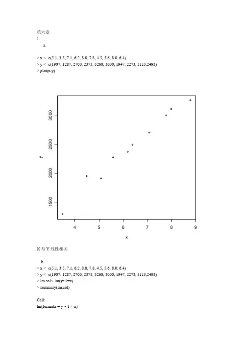
第六章 1. a .> x <- c(5.1, 3.5, 7.1, 6.2, 8.8, 7.8, 4.5, 5.6, 8.0, 6.4)> y <- c(1907, 1287, 2700, 2373, 3260, 3000, 1947, 2273, 3113,2493) > plot(x,y)456789150020002500300xyX 与Y 线性相关b .> x <- c(5.1, 3.5, 7.1, 6.2, 8.8, 7.8, 4.5, 5.6, 8.0, 6.4)> y <- c(1907, 1287, 2700, 2373, 3260, 3000, 1947, 2273, 3113,2493) > lm.sol<-lm(y~1+x) > summary(lm.sol) Call:lm(formula = y ~ 1 + x)Residuals:Min 1Q Median 3Q Max-128.591 -70.978 -3.727 49.263 167.228Coefficients:Estimate Std. Error t value Pr(>|t|)(Intercept) 140.95 125.11 1.127 0.293x 364.18 19.26 18.908 6.33e-08 ***---Signif. codes: 0 ‘***’ 0.001 ‘**’ 0.01 ‘*’ 0.05 ‘.’ 0.1 ‘ ’ 1Residual standard error: 96.42 on 8 degrees of freedomMultiple R-Squared: 0.9781, Adjusted R-squared: 0.9754F-statistic: 357.5 on 1 and 8 DF, p-value: 6.33e-08回归方程为Y=140.95+364.18X,极为显著d.> new <- data.frame(x=7)> lm.pred <- predict(lm.sol,new,interval="prediction",level=0.95)> lm.predfit lwr upr[1,] 2690.227 2454.971 2925.484Y(7)= 2690.227, [2454.971,2925.484]2.> out<-data.frame(+ x1 <- c(0.4,0.4,3.1,0.6,4.7,1.7,9.4,10.1,11.6,12.6,10.9,23.1,23.1,21.6,23.1,1.9,26.8,29.9), + x2 <- c(52,34,19,34,24,65,44,31,29,58,37,46,50,44,56,36,58,51),+ x3 <- c(158,163,37,157,59,123,46,117,173,112,111,114,134,73,168,143,202,124),+ y <- c(64,60,71,61,54,77,81,93,93,51,76,96,77,93,95,54,168,99)+ )> lm.sol<-lm(y~x1+x2+x3,data=out)> summary(lm.sol)Call:lm(formula = y ~ x1 + x2 + x3, data = out)Residuals:Min 1Q Median 3Q Max-27.575 -11.160 -2.799 11.574 48.808Coefficients:Estimate Std. Error t value Pr(>|t|)(Intercept) 44.9290 18.3408 2.450 0.02806 *x1 1.8033 0.5290 3.409 0.00424 **x2 -0.1337 0.4440 -0.301 0.76771x3 0.1668 0.1141 1.462 0.16573---Signif. codes: 0 ‘***’ 0.001 ‘**’ 0.01 ‘*’ 0.05 ‘.’ 0.1 ‘ ’ 1Residual standard error: 19.93 on 14 degrees of freedomMultiple R-Squared: 0.551, Adjusted R-squared: 0.4547F-statistic: 5.726 on 3 and 14 DF, p-value: 0.009004回归方程为y=44.9290+1.8033x1-0.1337x2+0.1668x3由计算结果可以得到,回归系数与回归方程的检验都是显著的3.a.> x<-c(1,1,1,1,2,2,2,3,3,3,4,4,4,5,6,6,6,7,7,7,8,8,8,9,11,12,12,12)> y<-c(0.6,1.6,0.5,1.2,2.0,1.3,2.5,2.2,2.4,1.2,3.5,4.1,5.1,5.7,3.4,9.7,8.6,4.0,5.5,10.5,17.5,13.4,4.5, + 30.4,12.4,13.4,26.2,7.4)> lm.sol <- lm(y ~ 1+x)> summary(lm.sol)Call:lm(formula = y ~ 1 + x)Residuals:Min 1Q Median 3Q Max-9.84130 -2.33691 -0.02137 1.05921 17.83201Coefficients:Estimate Std. Error t value Pr(>|t|)(Intercept) -1.4519 1.8353 -0.791 0.436x 1.5578 0.2807 5.549 7.93e-06 ***---Signif. codes: 0 ‘***’ 0.001 ‘**’ 0.01 ‘*’ 0.05 ‘.’ 0.1 ‘ ’ 1Residual standard error: 5.168 on 26 degrees of freedomMultiple R-Squared: 0.5422, Adjusted R-squared: 0.5246F-statistic: 30.8 on 1 and 26 DF, p-value: 7.931e-06线性回归方程为y=-1.4519+1.5578x,并且未通过t检验和F检验> plot(x,y)> abline(-1.4519,1.5578)>246810120510********xyc .> x<-c(1,1,1,1,2,2,2,3,3,3,4,4,4,5,6,6,6,7,7,7,8,8,8,9,11,12,12,12)> y<-c(0.6,1.6,0.5,1.2,2.0,1.3,2.5,2.2,2.4,1.2,3.5,4.1,5.1,5.7,3.4,9.7,8.6,4.0,5.5,10.5,17.5,13.4,4.5, + 30.4,12.4,13.4,26.2,7.4)> y.res<-resid(lm.sol);y.fit<-predict(lm.sol) > plot(y.res~y.fit)> y.rst<-rstandard(lm.sol) > plot(y.rst~y.fit) >普通残差051015-10-5051015y.fity .r e s标准化残差051015-2-10123y.fity .r s td . (4)> lm.new<-update(lm.data3,sqrt(.)~.);coef(lm.new) (Intercept) x 0.7665018 0.29136202x 0.084890650.4466549x 0.58752220.2913620x0.7665018 ++=+=∧∧y y> plot(x,y)> lines(x,y=0.5875222+0.08489065*x^2+0.4466549*x) > y.res<-resid(lm.new);y.fit<-predict(lm.new) > plot(y.res~y.fit)> y.rst<-rstandard(lm.new)> plot(y.rst~y.fit)4.> lm.sol<-lm(Y~X1+X2,data=toothpaste)> summary(lm.sol)Call:lm(formula = Y ~ X1 + X2, data = toothpaste)Residuals:Min 1Q Median 3Q Max-0.497785 -0.120312 -0.008672 0.110844 0.581059Coefficients:Estimate Std. Error t value Pr(>|t|)(Intercept) 4.4075 0.7223 6.102 1.62e-06 ***X1 1.5883 0.2994 5.304 1.35e-05 ***X2 0.5635 0.1191 4.733 6.25e-05 ***---Signif. codes: 0 ‘***’ 0.001 ‘**’ 0.01 ‘*’ 0.05 ‘.’ 0.1 ‘ ’ 1Residual standard error: 0.2383 on 27 degrees of freedomMultiple R-squared: 0.886, Adjusted R-squared: 0.8776F-statistic: 105 on 2 and 27 DF, p-value: 1.845e-13> source("Reg_Diag.R");Reg_Diag(lm.sol)residual s1 standard s2 student s3 hat_matrix s4 DFFITS1 -0.047231639 -0.21248023 -0.20868284 0.13012303 -0.080711402 -0.098070223 -0.42151698 -0.41500522 0.04704358 -0.092207713 0.074288624 0.33492116 0.32934525 0.13385955 0.129473814 -0.006645926 -0.03003380 -0.02947287 0.13797634 -0.011791395 0.581059204 * 2.55701395 * 2.88236603 * 0.09091719 0.911528866 -0.107785364 -0.46031439 -0.45349258 0.03475104 -0.086046747 0.300758350 1.31532456 1.33418993 0.07955382 0.392237398 0.424810360 2.05723960 * 2.19842345 * 0.24932956 * 1.266991129 -0.027532493 -0.12804079 -0.12568545 0.18600211 -0.0600803310 -0.026629932 -0.11546376 -0.11333335 0.06356511 -0.0295276111 -0.497785364 -2.12587089 * -2.28622467 * 0.03475104 -0.4337935912 0.061913782 0.26540305 0.26078220 0.04194215 0.0545641513 0.112816344 0.48968055 0.48267493 0.06556908 0.1278588114 -0.150249714 -0.65395500 -0.64687388 0.07069034 -0.1784101015 0.104927089 0.45112292 0.44436784 0.04761107 0.0993549316 0.154341375 0.66319490 0.65616401 0.04652075 0.1449372917 0.057639541 0.25360011 0.24915642 0.09056633 0.0786266818 -0.146012230 -0.64156026 -0.63442169 0.08813106 -0.1972315219 -0.124487198 -0.53776150 -0.53055795 0.05659354 -0.1299471720 -0.040713930 -0.18584177 -0.18248454 0.15505538 -0.0781727521 -0.199843357 -0.88485598 -0.88118586 0.10202733 -0.2970258322 -0.359558498 -1.59386063 -1.64328265 0.10408399 -0.5601064823 -0.387785364 -1.65609855 -1.71455446 0.03475104 -0.3253235524 -0.010697936 -0.04979066 -0.04886215 0.18729463 -0.0234568025 -0.283315771 -1.25181018 -1.26568782 0.09823492 -0.4177465226 0.017855655 0.08230563 0.08077720 0.17144488 0.0367443327 0.279286070 1.27482211 1.29043074 0.15505538 0.5527948628 0.022483501 0.09864705 0.09682047 0.08548985 0.0296026229 0.174895100 0.76513625 0.75910825 0.08017207 0.2241103830 0.147269942 0.66281470 0.65578162 0.13089383 0.25449685s5 cooks_distance s6 COVRATIO s71 2.251190e-03 1.28095242 2.923723e-03 1.15211573 5.778631e-03 1.27690564 4.812656e-05 1.29899825 * 2.179654e-01 0.5361673 *6 2.542824e-03 1.13309647 4.984335e-02 0.99745488 * 4.685683e-01 * 0.89452379 1.248734e-03 1.373272210 3.016556e-04 1.194126111 5.423517e-02 0.669681912 1.027897e-03 1.159781213 5.608624e-03 1.166813514 1.084362e-02 1.148706415 3.391268e-03 1.149474316 7.153137e-03 1.118050417 2.134879e-03 1.222624518 1.326021e-02 1.172800619 5.782640e-03 1.149323820 2.112633e-03 1.320308321 2.965359e-02 1.141740222 9.837757e-02 0.929311223 3.291392e-02 0.841337024 1.904437e-04 1.377585325 5.690208e-02 1.037953426 4.672410e-04 1.350588127 9.941147e-02 1.100173228 3.032306e-04 1.223243929 1.700877e-02 1.139997330 2.205512e-02 1.2266609> toothpaste<-data.frame(+ X1=c(-0.05, 0.25,0.60,0,0.20, 0.15,-0.15, 0.15,+ 0.10,0.40,0.45,0.35,0.30, 0.50,0.50, 0.40,-0.05,+ -0.05,-0.10,0.20,0.10,0.50,0.60,-0.05,0, 0.05, 0.55), + X2=c( 5.50,6.75,7.25,5.50,6.50,6.75,5.25,6.00,+ 6.25,7.00,6.90,6.80,6.80,7.10,7.00,6.80,6.50,+ 6.25,6.00,6.50,7.00,6.80,6.80,6.50,5.75,5.80,6.80), + Y =c( 7.38,8.51,9.52,7.50,8.28,8.75,7.10,8.00,+ 8.15,9.10,8.86,8.90,8.87,9.26,9.00,8.75,7.95,+ 7.65,7.27,8.00,8.50,8.75,9.21,8.27,7.67,7.93,9.26) + )>> lm.sol<-lm(Y~X1+X2,data=toothpaste)> summary(lm.sol)Call:lm(formula = Y ~ X1 + X2, data = toothpaste)Residuals:Min 1Q Median 3Q Max-0.37130 -0.10114 0.03066 0.10016 0.30162Coefficients:Estimate Std. Error t value Pr(>|t|) (Intercept) 4.0759 0.6267 6.504 1.00e-06 ***X1 1.5276 0.2354 6.489 1.04e-06 ***X2 0.6138 0.1027 5.974 3.63e-06 ***---Signif. codes: 0 ‘***’ 0.001 ‘**’ 0.01 ‘*’ 0.05 ‘.’ 0.1 ‘ ’ 1Residual standard error: 0.1767 on 24 degrees of freedom Multiple R-squared: 0.9378, Adjusted R-squared: 0.9327F-statistic: 181 on 2 and 24 DF, p-value: 3.33e-155.XX<-cor(cement[1:4])kappa(XX,exact=TRUE)[1] 1376.881> eigen(XX)$values[1] 2.235704035 1.576066070 0.186606149 0.001623746$vectors[,1] [,2] [,3] [,4][1,] -0.4759552 0.5089794 0.6755002 0.2410522[2,] -0.5638702 -0.4139315 -0.3144204 0.6417561[3,] 0.3940665 -0.6049691 0.6376911 0.2684661[4,] 0.5479312 0.4512351 -0.1954210 0.6767340删去了X3,X4> cement<-data.frame(+ X1=c( 7, 1, 11, 11, 7, 11, 3, 1, 2, 21, 1, 11, 10),+ X2=c(26, 29, 56, 31, 52, 55, 71, 31, 54, 47, 40, 66, 68),+ Y =c(78.5, 74.3, 104.3, 87.6, 95.9, 109.2, 102.7, 72.5, + 93.1,115.9, 83.8, 113.3, 109.4)+ )> XX<-cor(cement[1:2])> kappa(XX,exact=TRUE)[1] 1.592620复共线性消失了。
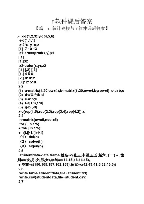
r软件课后答案【篇一:统计建模与r软件课后答案】> x-c(1,2,3);y-c(4,5,6)e-c(1,1,1)z-2*x+y+e;z[1] 7 10 13z1-crossprod(x,y);z1[,1][1,]32z2-outer(x,y);z2[,1] [,2] [,3][1,] 4 5 6[2,] 81012[3,]1215182.2(1) a-matrix(1:20,ow=4);b-matrix(1:20,ow=4,byrow=t) c-a+b;c(2) d-a%*%b;d(3) e-a*b;e(4) f-a[1:3,1:3](5) g-b[,-3]x-c(rep(1,5),rep(2,3),rep(3,4),rep(4,2));x2.4h-matrix(ow=5,ncol=5)for (i in 1:5)+ for(j in 1:5)+ h[i,j]-1/(i+j-1)(1) det(h)(2) solve(h)(3) eigen(h)2.5studentdata-data.frame(姓名=c(张三,李四,王五,赵六,丁一) + ,性别=c(女,男,女,男,女),年龄=c(14,15,16,14,15),+ 身高=c(156,165,157,162,159),体重=c(42,49,41.5,52,45.5))2.6write.table(studentdata,file=student.txt)write.csv(studentdata,file=student.csv)2.7count-function(n){if (n=0)print(要求输入一个正整数)repeat{if (n%%2==0)n-n/2elsen-(3*n+1)if(n==1)break}print(运算成功)}}第三章3.1首先将数据录入为x。
利用data_outline函数。
如下 data_outline(x)3.2hist(x,freq=f)lines(density(x),col=red)y-min(x):max(x)lines(y,dnorm(y,73.668,3.9389),col=blue)plot(ecdf(x),verticals=t,do.p=f)lines(y,pnorm(y,73.668,3.9389))qqnorm(x)qqline(x)3.3stem(x)boxplot(x)fivenum(x)3.4shapiro.test(x)ks.test(x,pnorm,73.668,3.9389)one-sample kolmogorov-smirnov testdata: xd = 0.073, p-value = 0.6611alternative hypothesis: two-sidedwarning message:in ks.test(x, pnorm, 73.668, 3.9389) :ties should not be present for the kolmogorov-smirnov test这里出现警告信息是因为ks检验要求样本数据是连续的,不允许出现重复值3.5x1-c(2,4,3,2,4,7,7,2,2,5,4);x2-c(5,6,8,5,10,7,12,12,6,6);x3-c(7,11,6,6,7,9,5,5,10,6,3,10)boxplot(x1,x2,x3,names=c(x1,x2,x3),vcol=c(2,3,4))windows()plot(factor(c(rep(1,length(x1)),rep(2,length(x2)),rep(3,length(x3) ))),c(x1,x2,x3))3.6rubber-data.frame(x1=c(65,70,70,69,66,67,68,72,66,68),+x2=c(45,45,48,46,50,46,47,43,47,48),x3=c(27.6,30.7,31.8,32.6,31 .0,31.3,37.0,33.6,33.1,34.2))plot(rubber)【篇二:r软件课后习题第五章】> ####写出求正态总体均值检验的r程序(程序名:mean.test1.r) mean.test1-function(x, mu=0, sigma=-1, side=0){source(p_value.r)n-length(x); xb-mean(x)if (sigma0){z-(xb-mu)/(sigma/sqrt(n))p-p_value(pnorm, z, side=side)data.frame(mean=xb, df=n, z=z, p_value=p)}else{t-(xb-mu)/(sd(x)/sqrt(n))p-p_value(pt, t, paramet=n-1, side=side)data.frame(mean=xb, df=n-1, t=t, p_value=p)}}####写出求p值的r程序(程序名:p_value.r)p_value-function(cdf, x, paramet=numeric(0), side=0){n-length(paramet)p-switch(n+1,cdf(x),cdf(x, paramet),cdf(x, paramet[1], paramet[2]),cdf(x, paramet[1], paramet[2], paramet[3]))if (side0) pelse if (side0) 1-pelseif (p1/2) 2*pelse 2*(1-p)}####输入数据,再调用函数mean.test1()x-c(220,188,162,230,145,160,238,188,247,113,126,245,164,231,256 ,183,190,158,224,175) source(mean.test1.r)a-mean.test1(x, mu=225,side=0)a得到:mean dft p_value1 192.15 19 -3.478262 0.002516436可知,p值小于0.05,故与正常值存在差异5.2####输入数据,再调用函数mean.test1()x-c(1067,919,1196,785,1126,936,918,1156,920,948)source(mean.test1.r)mean.test1(x, mu=1000,side=1)得到:mean df tp_value1 997.1 9 -0.06971322 0.5270268所以灯泡寿命为1000小时以上的概率是0.47297325.3####写出两总体均值检验的r程序(程序名:mean.test2.r)mean.test2-function(x, y,sigma=c(-1, -1), var.equal=false, side=0){source(p_value.r)n1-length(x); n2-length(y)xb-mean(x); yb-mean(y)if (all(sigma0)){z-(xb-yb)/sqrt(sigma[1]^2/n1+sigma[2]^2/n2)p-p_value(pnorm, z, side=side)data.frame(mean=xb-yb, df=n1+n2, z=z, p_value=p)}else{if (var.equal == true){sw-sqrt(((n1-1)*var(x)+(n2-1)*var(y))/(n1+n2-2))t-(xb-yb)/(sw*sqrt(1/n1+1/n2))nu-n1+n2-2}else{s1-var(x); s2-var(y)nu-(s1/n1+s2/n2)^2/(s1^2/n1^2/(n1-1)+s2^2/n2^2/(n2-1)) t-(xb-yb)/sqrt(s1/n1+s2/n2)}p-p_value(pt, t, paramet=nu, side=side)data.frame(mean=xb-yb, df=nu, t=t, p_value=p)}}####输入数据,再调用函数mean.test2()x-c(113,120,138,120,100,118,138,123)y-c(138,116,125,136,110,132,130,110)source(mean.test2.r)mean.test2(x, y, var.equal=true, side=0)得到:mean df tp_value1 -3.375 14 -0.5659672 0.5803752p值大于0.05,故接受原假设5.4####写出均值已知和均值未知两种情况方差比检验的r程序(程序名:var.test2.r)var.test2-function(x, y,mu=c(inf,inf),side=0){source(p_value.r)n1-length(x); n2-length(y)if (all(all(muinf)){sx2-sum((x-mu[1])^2)/n1;sy2-sum((y-mu[2])^2)/n2df1=n1;df2=n2}else{sx2-var(x); sy2-var(y);df1=n1-1;df2=n2-1}r-sx2/sy2p-p_value(pf, r, paramet=c(df1,df2), side=side)data.frame(rate=r, df1=df1, df2=df2,f=f, p_value=p)}}####输入数据x-c(-0.70,-5.60,2.00,2.80,0.70,3.50,4.00,5.80,7.10,-0.50,2.50,-1.60,1.70,3.00,0.40,4.50,4.60,2.50,6.00,-1.40)a-shapiro.test(x)ashapiro-wilk normality testdata: xw = 0.9699, p-value = 0.75270.05y-c(3.70,6.50,5.00,5.20,0.80,0.20,0.60,3.40,6.60,-1.10,6.00,3.80,2.00,1.60,2.00,2.20,1.20,3.10,1.70,-2.00)b-shapiro.test(y)bshapiro-wilk normality testdata: yw = 0.971, p-value = 0.77540.05由以上可知,两组数据均为正态分布####输入数据,再调用函数mean.test2()x-c(-0.70,-5.60,2.00,2.80,0.70,3.50,4.00,5.80,7.10,-0.50,2.50,-1.60,1.70,3.00,0.40,4.50,4.60,2.50,6.00,-1.40)y-c(3.70,6.50,5.00,5.20,0.80,0.20,0.60,3.40,6.60,-1.10,6.00,3.80,2.00,1.60,2.00,2.20,1.20,3.10,1.70,-2.00)source(mean.test2.r)a-mean.test2(x, y, var.equal=true, side=0);amean dftp_value1 -0.56 38 -0.641872 0.5248097b-mean.test2(x, y, var.equal=false, side=0);bmean dft p_value1 -0.56 36.08632 -0.641872 0.525013c-t.test(x-y, alternative = two.sided);cone sample t-testdata: x - yt = -0.6464, df = 19, p-value = 0.5257alternative hypothesis: true mean is not equal to 095 percent confidence interval:-2.373146 1.253146sample estimates:mean of x-0.56以上p值均大于0.05,故均值无差异。
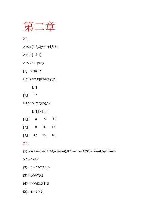
第二章2.1> x<-c(1,2,3);y<-c(4,5,6)> e<-c(1,1,1)> z<-2*x+y+e;z[1] 7 10 13> z1<-crossprod(x,y);z1[,1][1,] 32> z2<-outer(x,y);z2[,1] [,2] [,3][1,] 4 5 6[2,] 8 10 12[3,] 12 15 182.2(1)> A<-matrix(1:20,nrow=4);B<-matrix(1:20,nrow=4,byrow=T) > C<-A+B;C(2)> D<-A%*%B;D(3)> E<-A*B;E(4)> F<-A[1:3,1:3](5)> G<-B[,-3]> x<-c(rep(1,5),rep(2,3),rep(3,4),rep(4,2));x2.4> H<-matrix(nrow=5,ncol=5)> for (i in 1:5)+ for(j in 1:5)+ H[i,j]<-1/(i+j-1)(1)> det(H)(2)> solve(H)(3)> eigen(H)2.5> studentdata<-data.frame(姓名=c('张三','李四','王五','赵六','丁一')+ ,性别=c('女','男','女','男','女'),年龄=c('14','15','16','14','15'),+ 身高=c('156','165','157','162','159'),体重=c('42','49','41.5','52','45.5')) 2.6> write.table(studentdata,file='student.txt')> write.csv(studentdata,file='student.csv')2.7count<-function(n){if (n<=0)print('要求输入一个正整数')repeat{if (n%%2==0)n<-n/2elsen<-(3*n+1)if(n==1)break}print('运算成功')}}第三章3.1首先将数据录入为x。
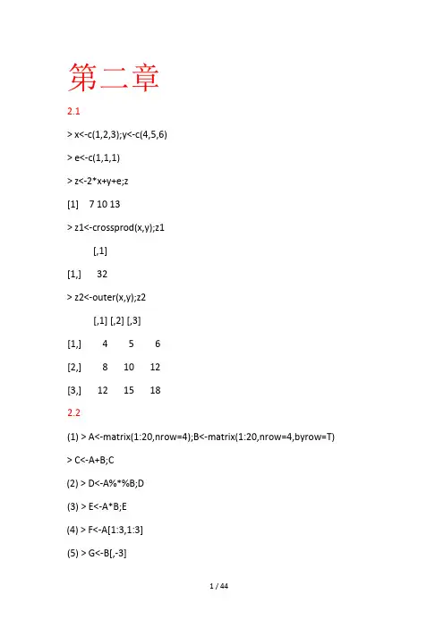
第二章2.1> x<-c(1,2,3);y<-c(4,5,6)> e<-c(1,1,1)> z<-2*x+y+e;z[1] 7 10 13>z1<-crossprod(x,y);z1[,1][1,] 32>z2<-outer(x,y);z2[,1] [,2] [,3][1,] 4 5 6[2,] 8 10 12[3,] 12 15 182.2(1) > A<-matrix(1:20,nrow=4);B<-matrix(1:20,nrow=4,byrow=T) >C<-A+B;C(2) > D<-A%*%B;D(3) > E<-A*B;E(4) > F<-A[1:3,1:3](5) > G<-B[,-3]2.3>x<-c(rep(1,5),rep(2,3),rep(3,4),rep(4,2));x2.4>H<-matrix(nrow=5,ncol=5)>for (i in 1:5)+ for(j in 1:5)+ H[i,j]<-1/(i+j-1)(1)> det(H)(2)> solve(H)(3)> eigen(H)2.5>studentdata<-data.frame(姓名=c('张三','李四','王五','赵六','丁一') + ,性别=c('女','男','女','男','女'),年龄=c('14','15','16','14','15'),+ 身高=c('156','165','157','162','159'),体重=c('42','49','41.5','52','45.5')) 2.6>write.table(studentdata,file='student.txt')>write.csv(studentdata,file='student.csv')2.7count<-function(n){if (n<=0)print('要求输入一个正整数')else{ repeat{if (n%%2==0)n<-n/2elsen<-(3*n+1)if(n==1)break}print('运算成功')}}第三章3.1首先将数据录入为x。
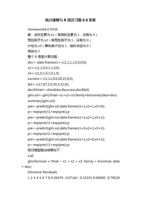
统计建模与R语言习题6.6答案Homework6.6 P333解:设抗生素为x1(有用抗生素为1,没有为0)危险因子为x2(有危险因子为1,没有为0)计划为x3(事先有计划为1,临时决定为0)感染为Y整个R语言计算过程:doc<-data.frame(x1<-c(1,1,1,1,0,0,0,0),x2<-c(1,1,0,0,1,1,0,0),x3<-c(1,0,1,0,1,0,1,0) ,success<-c(1,11,0,0,28,23,8,0),fail<-c(17,87,2,0,30,3,32,9))doc$Ymat<-cbind(doc$success,doc$fail)glm.sol<-glm(Ymat~x1+x2+x3,family=binomial,data=doc) summary(glm.sol)pre<-predict(glm.sol,data.frame(x1=1,x2=1,x3=0))p<-exp(pre)/(1+exp(pre));ppre<-predict(glm.sol,data.frame(x1=1,x2=1,x3=1))p<-exp(pre)/(1+exp(pre));ppre<-predict(glm.sol,data.frame(x1=0,x2=1,x3=1))p<-exp(pre)/(1+exp(pre));ppre<-predict(glm.sol,data.frame(x1=1,x2=0,x3=1))p<-exp(pre)/(1+exp(pre));p回归模型输出结果如下:Call:glm(formula = Ymat ~ x1 + x2 + x3, family = binomial, data = doc)Deviance Residuals:1 2 3 4 5 6 7 8 0.26470 -0.07162 -0.15231 0.00000 -0.785201.49623 1.21563 -2.56229 Coefficients:Estimate Std. Error z value Pr(>|z|)(Intercept) -0.8207 0.4947 -1.659 0.0971 .x1 -3.2544 0.4813 -6.761 1.37e-11 ***x2 2.0299 0.4553 4.459 8.25e-06 ***x3 -1.0720 0.4254 -2.520 0.0117 *---Signif. codes: 0 ‘***’ 0.001 ‘**’ 0.01 ‘*’ 0.05 ‘.’ 0.1 ‘ ’ 1(Dispersion parameter for binomial family taken to be 1)Null deviance: 83.491 on 6 degrees of freedomResidual deviance: 10.997 on 3 degrees of freedomAIC: 36.178Number of Fisher Scoring iterations: 5从上述结果即有常数项以及x项的系数β分别为-0.8207,-3.2544, 2.0299,-1.0720,并且回归方程通过检验得到回归模型:P=exp(-0.8207-3.2544x1+2.0299x2-1.0720x3)/(1+exp(-0.8207-3.2544x1+2.0299x2-1.0720x3))假设医生需要对一产妇进行剖腹手术,令x1=1,x2=1,x3=0即在手术中是用抗生素且有危险因子和临时决定进行手术,那么pre<-predict(glm.sol,data.frame(x1=1,x2=1,x3=0))p<-exp(pre)/(1+exp(pre));p10.1145421即11.4521%,也就是说在临时决定进行手术的感染率为11.4521% 那么当x3=1时pre<-predict(glm.sol,data.frame(x1=1,x2=1,x3=1))> p<-exp(pre)/(1+exp(pre));p10.04240619即4.240619%,也就是说在事先有计划进行手术的感染率为4.240619%。
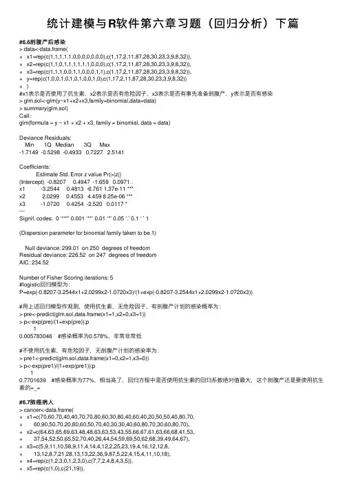
统计建模与R软件第六章习题(回归分析)下篇#6.6剖腹产后感染> data<-data.frame(+ x1=rep(c(1,1,1,1,1,0,0,0,0,0,0,0),c(1,17,2,11,87,28,30,23,3,9,8,32)),+ x2=rep(c(1,1,0,1,1,1,1,1,1,0,0,0),c(1,17,2,11,87,28,30,23,3,9,8,32)),+ x3=rep(c(1,1,1,0,0,1,1,0,0,0,1,1),c(1,17,2,11,87,28,30,23,3,9,8,32)),+ y=rep(c(1,0,0,1,0,1,0,1,0,0,1,0),c(1,17,2,11,87,28,30,23,3,9,8,32))+ )#x1表⽰是否使⽤了抗⽣素,x2表⽰是否有危险因⼦,x3表⽰是否有事先准备剖腹产,y表⽰是否有感染> glm.sol<-glm(y~x1+x2+x3,family=binomial,data=data)> summary(glm.sol)Call:glm(formula = y ~ x1 + x2 + x3, family = binomial, data = data)Deviance Residuals:Min 1Q Median 3Q Max-1.7149 -0.5298 -0.4933 0.7227 2.5141Coefficients:Estimate Std. Error z value Pr(>|z|)(Intercept) -0.8207 0.4947 -1.659 0.0971 .x1 -3.2544 0.4813 -6.761 1.37e-11 ***x2 2.0299 0.4553 4.459 8.25e-06 ***x3 -1.0720 0.4254 -2.520 0.0117 *---Signif. codes: 0 ‘***’ 0.001 ‘**’ 0.01 ‘*’ 0.05 ‘.’ 0.1 ‘ ’ 1(Dispersion parameter for binomial family taken to be 1)Null deviance: 299.01 on 250 degrees of freedomResidual deviance: 226.52 on 247 degrees of freedomAIC: 234.52Number of Fisher Scoring iterations: 5#logistic回归模型为:P=exp(-0.8207-3.2544x1+2.0299x2-1.0720x3)/(1+exp(-0.8207-3.2544x1+2.0299x2-1.0720x3))#⽤上述回归模型作观测,使⽤抗⽣素,⽆危险因⼦,有剖腹产计划的感染概率为:> pre<-predict(glm.sol,data.frame(x1=1,x2=0,x3=1))> p<-exp(pre)/(1+exp(pre));p10.005783046 #感染概率为0.578%,⾮常⾮常低#不使⽤抗⽣素,有危险因⼦,⽆剖腹产计划的感染率为:> pre1<-predict(glm.sol,data.frame(x1=0,x2=1,x3=0))> p<-exp(pre1)/(1+exp(pre1));p10.7701639 #感染概率为77%,相当⾼了,回归⽅程中是否使⽤抗⽣素的回归系数绝对值最⼤,这个剖腹产还是要使⽤抗⽣素的=_=#6.7肺癌病⼈> cancer<-data.frame(+ x1=c(70,60,70,40,40,70,70,80,60,30,80,40,60,40,20,50,50,40,80,70,+ 60,90,50,70,20,80,60,50,70,40,30,30,40,60,80,70,30,60,80,70),+ x2=c(64,63,65,69,63,48,48,63,63,53,43,55,66,67,61,63,66,68,41,53,+ 37,54,52,50,65,52,70,40,26,44,54,59,69,50,62,68,39,49,64,67),+ x3=c(5,9,11,10,58,9,11,4,14,4,12,2,25,23,19,4,16,12,12,8,+ 13,12,8,7,21,28,13,13,22,36,9,87,5,22,4,15,4,11,10,18),+ x4=rep(c(1,2,3,0,1,2,3,0),c(7,7,2,4,8,4,3,5)),+ x5=rep(c(1,0),c(21,19)),+ y=rep(c(1,0,1,0,1,0,1,0,1,0,1),c(1,11,1,5,2,1,3,1,1,12,2))+ )#x1表⽰⽣活⾏动能⼒评分,x2表⽰病⼈年龄,x3表⽰由诊断到直⼊研究时间(⽉),x4表⽰肿瘤类型(0是磷癌,1是⼩型细胞癌,2是腺癌,3是⼤型细胞癌),x5表⽰两种化疗⽅法(1是常规,0是试验新法),y表⽰病⼈的⽣存时间(0是⽣存时间短,⼩于200天;1是⽣存时间长,⼤于等于200天)6.7.1logistic回归模型> glm.c<-glm(y~x1+x2+x3+x4+x5,family=binomial,data=cancer)> summary(glm.c)Call:glm(formula = y ~ x1 + x2 + x3 + x4 + x5, family = binomial,data = cancer)Deviance Residuals:Min 1Q Median 3Q Max-1.73402 -0.64522 -0.22773 0.09734 2.21941Coefficients:Estimate Std. Error z value Pr(>|z|)(Intercept) -7.22297 4.39926 -1.642 0.1006x1 0.10048 0.04322 2.325 0.0201 *x2 0.01716 0.04417 0.389 0.6976x3 0.01828 0.05405 0.338 0.7353x4 -1.07233 0.58653 -1.828 0.0675 .x5 -0.62473 0.96204 -0.649 0.5161---Signif. codes: 0 ‘***’ 0.001 ‘**’ 0.01 ‘*’ 0.05 ‘.’ 0.1 ‘ ’ 1(Dispersion parameter for binomial family taken to be 1)Null deviance: 44.987 on 39 degrees of freedomResidual deviance: 28.329 on 34 degrees of freedomAIC: 40.329Number of Fisher Scoring iterations: 6#模型不显著,肿瘤类型x4与化疗⽅法x5应该是主要的影响因素#计算各病⼈⽣存时间⼤于等于200天的概率估计值> n=c(cancer$y==1)> n[1] TRUE FALSE FALSE FALSE FALSE FALSE FALSE FALSE FALSE FALSE FALSE FALSE TRUE[14] FALSE FALSE FALSE FALSE FALSE TRUE TRUE FALSE TRUE TRUE TRUE FALSE TRUE[27] FALSE FALSE FALSE FALSE FALSE FALSE FALSE FALSE FALSE FALSE FALSE FALSE TRUE[40] TRUE> pre=glm.c$fitted[n];pre1 13 19 20 22 23 240.33257413 0.08518899 0.75283057 0.56015746 0.86922215 0.09686322 0.4315437926 39 400.75903351 0.89058079 0.78407564> p=exp(pre)/(1+exp(pre));p1 13 19 20 22 23 24 260.5823856 0.5212844 0.6797952 0.6364890 0.7045838 0.5241969 0.6062422 0.681143939 400.7090100 0.68655786.7.2逐步回归法选取⾃变量> ew<-step(glm.c)Start: AIC=40.33y ~ x1 + x2 + x3 + x4 + x5Df Deviance AIC- x3 1 28.430 38.430- x2 1 28.484 38.484- x5 1 28.750 38.75028.329 40.329- x4 1 32.483 42.483- x1 1 38.297 48.297Step: AIC=38.43y ~ x1 + x2 + x4 + x5Df Deviance AIC- x2 1 28.564 36.564- x5 1 28.955 36.95528.430 38.430- x4 1 32.563 40.563- x1 1 38.474 46.474Step: AIC=36.56y ~ x1 + x4 + x5Df Deviance AIC- x5 1 29.073 35.07328.564 36.564- x4 1 32.892 38.892- x1 1 38.478 44.478Step: AIC=35.07y ~ x1 + x4Df Deviance AIC29.073 35.073- x4 1 33.535 37.535- x1 1 39.131 43.131#剩下x1与x4⾃变量> summary(ew)Call:glm(formula = y ~ x1 + x4, family = binomial, data = cancer) Deviance Residuals:Min 1Q Median 3Q Max-1.4825 -0.6617 -0.1877 0.1227 2.2844Coefficients:Estimate Std. Error z value Pr(>|z|)(Intercept) -6.13755 2.73844 -2.241 0.0250 *x1 0.09759 0.04079 2.393 0.0167 *x4 -1.12524 0.60239 -1.868 0.0618 .---Signif. codes: 0 ‘***’ 0.001 ‘**’ 0.01 ‘*’ 0.05 ‘.’ 0.1 ‘ ’ 1 (Dispersion parameter for binomial family taken to be 1)Null deviance: 44.987 on 39 degrees of freedomResidual deviance: 29.073 on 37 degrees of freedomAIC: 35.073Number of Fisher Scoring iterations: 6#模型显著性提⾼#计算逐步回归后新模型各病⼈⽣存时间⼤于等于200天的概率估计值> pre1=ew$fitted[n];pre11 13 19 20 22 23 240.39371565 0.07358866 0.84149409 0.66674959 0.82054044 0.08444317 0.3937156526 39 400.63277649 0.84149409 0.66674959> p1=exp(pre1)/(1+exp(pre1));p11 13 19 20 22 23 24 260.5971768 0.5183889 0.6987798 0.6607750 0.6943510 0.5210983 0.5971768 0.653118839 400.6987798 0.6607750#6.8⾃动咖啡售货机与咖啡销售> x<-c(0,0,1,1,2,2,3,3,4,4,5,5,6,6) #咖啡机数量> y<-c(508.1,498.4,568.2,577.3,651.7,657,713.4,697.5,755.3,758.9,787.6,792.1,841.4,831.8) #咖啡销量6.8.1线性回归模型> lm.coffee<-lm(y~x)> summary(lm.coffee)Call:lm(formula = y ~ x)Residuals:Min 1Q Median 3Q Max-25.400 -11.484 -3.779 14.629 24.921Coefficients:Estimate Std. Error t value Pr(>|t|)(Intercept) 523.800 8.474 61.81 < 2e-16 ***x 54.893 2.350 23.36 2.26e-11 ***---Signif. codes: 0 ‘***’ 0.001 ‘**’ 0.01 ‘*’ 0.05 ‘.’ 0.1 ‘ ’ 1Residual standard error: 17.59 on 12 degrees of freedomMultiple R-squared: 0.9785, Adjusted R-squared: 0.9767F-statistic: 545.5 on 1 and 12 DF, p-value: 2.265e-11#线性回归⽅程为y=523.800+54.893x6.8.2多项式回归模型> plot(x,y)#从散点图上看,⽤⼆次曲线拟合更好> lm.coffee1<-lm(y~x+I(x^2))> summary(lm.coffee1)Call:lm(formula = y ~ x + I(x^2))Residuals:Min 1Q Median 3Q Max-10.6643 -5.6622 -0.4655 5.5000 10.6679Coefficients:Estimate Std. Error t value Pr(>|t|)(Intercept) 502.5560 4.8500 103.619 < 2e-16 ***x 80.3857 3.7861 21.232 2.81e-10 ***I(x^2) -4.2488 0.6063 -7.008 2.25e-05 ***---Signif. codes: 0 ‘***’ 0.001 ‘**’ 0.01 ‘*’ 0.05 ‘.’ 0.1 ‘ ’ 1Residual standard error: 7.858 on 11 degrees of freedomMultiple R-squared: 0.9961, Adjusted R-squared: 0.9953F-statistic: 1391 on 2 and 11 DF, p-value: 5.948e-14#多项式回归⽅程为:y=502.5560+80.3857x-4.2488x^2 相⽐线性回归,残差标准误降低,R平⽅达到0.99616.8.3画出散点图与拟合曲线> plot(x,y)> xfit<-seq(0,6,0.01)> yfit<-predict(lm.coffee1,data.frame(x=xfit))> lines(xfit,yfit)#6.9重伤病⼈出院后恢复情况> x<-c(2,5,7,10,14,19,26,31,34,38,45,52,53,60,65) #住院天数> y<-c(54,50,45,37,35,25,20,16,18,13,8,11,8,4,6) #预后指数6.9.1内在线性模型⽅法> plot(x,y)> lm.patient<-lm(log(y)~x)> summary(lm.patient)Call:lm(formula = log(y) ~ x)Residuals:Min 1Q Median 3Q Max-0.37241 -0.07073 0.02777 0.05982 0.33539Coefficients:Estimate Std. Error t value Pr(>|t|)(Intercept) 4.037159 0.084103 48.00 5.08e-16 ***x -0.037974 0.002284 -16.62 3.86e-10 ***---Signif. codes: 0 ‘***’ 0.001 ‘**’ 0.01 ‘*’ 0.05 ‘.’ 0.1 ‘ ’ 1Residual standard error: 0.1794 on 13 degrees of freedomMultiple R-squared: 0.9551, Adjusted R-squared: 0.9516F-statistic: 276.4 on 1 and 13 DF, p-value: 3.858e-10#线性回归⽅程为:lny=4.037159-0.037974x#计算估计值> yev=exp(4.037159)*exp(-0.037974*x);yev[1] 52.520890 46.865838 43.438277 38.761171 33.298855 27.540372 21.111861 17.460916 [9] 15.580856 13.385165 10.260781 7.865696 7.572604 5.804996 4.8011196.9.2⽤⾮线性⽅法计算估计值> nls.patient<-nls(y~a*exp(b*x),start=list(a=10,b=-0.01))> summary(nls.patient)Formula: y ~ a * exp(b * x)Parameters:Estimate Std. Error t value Pr(>|t|)a 58.606568 1.472160 39.81 5.70e-15 ***b -0.039586 0.001711 -23.13 6.01e-12 ***---Signif. codes: 0 ‘***’ 0.001 ‘**’ 0.01 ‘*’ 0.05 ‘.’ 0.1 ‘ ’ 1Residual standard error: 1.951 on 13 degrees of freedomNumber of iterations to convergence: 6Achieved convergence tolerance: 5.107e-07#⾮线性模型为:y=58.606568 * exp(-0.039586 * x)#计算估计值> yev=58.606568 * exp(-0.039586 * x);yev[1] 54.145495 48.082427 44.422441 39.448135 33.671197 27.624768 20.938944 17.178881 [9] 15.255236 13.021200 9.869772 7.481062 7.190702 5.450388 4.471647#使⽤nlm( )函数> fn<-function(p,X,Y)+ {+ f<-Y-p[1]*exp(p[2]*X)+ res<-sum(f^2)+ f1<-exp(p[2]*X)+ f2<-p[1]*exp(p[2]*X)*X+ J<-cbind(f1,f2)+ res+ }> nlm(fn,p=c(50, -0.01),x,y,hessian=TRUE)$minimum[1] 49.4593$estimate[1] 58.60712251 -0.03958742$gradient[1] -1.774625e-05 -9.522651e-03$hessian[,1] [,2][1,] 7.022561 4285.646[2,] 4285.646407 5161077.388$code[1] 2$iterations[1] 33#计算估计值> yev=58.60712251*exp(-0.03958742*x);yev[1] 54.145853 48.082541 44.422420 39.447948 33.670846 27.624284 20.938369 17.178287 [9] 15.254644 13.020620 9.869235 7.480580 7.190229 5.449975 4.471276#来看下估计值与实际值的差> y-yev[1] -0.14585337 1.91745922 0.57758014 -2.44794812 1.32915418 -2.62428435[7] -0.93836901 -1.17828719 2.74535642 -0.02062025 -1.86923491 3.51941952[13] 0.80977134 -1.44997507 1.52872352。

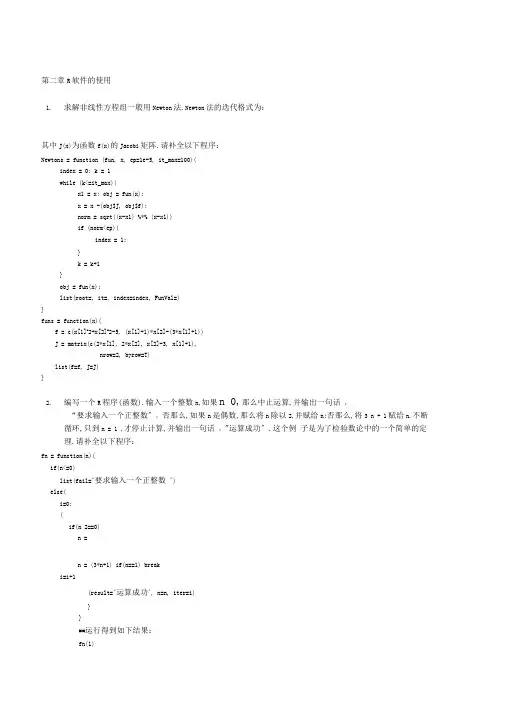
第二章R软件的使用1.求解非线性方程组一般用Newton法.Newton法的迭代格式为:其中J(x)为函数f(x)的Jacobi矩阵.请补全以下程序:Newtons = function (fun, x, ep=1e-5, it_max=100)(index = 0; k = 1while (k<=it_max)(x1 = x; obj = fun(x);x = x -(obj$J, obj$f);norm = sqrt((x-x1) %*% (x-x1))if (norm<ep)(index = 1;}k = k+1}obj = fun(x);list(root=, it=, index=index, FunVal=)}funs = function(x)(f = c(x[1]A2+x[2]A2-5, (x[1]+1)*x[2]-(3*x[1]+1))J = matrix(c(2*x[1], 2*x[2], x[2]-3, x[1]+1),nrow=2, byrow=T)list(f=f, J=J)}n 0,那么中止运算,并输出一句话:2.编写一个R程序(函数).输入一个整数n,如果“要求输入一个正整数〞;否那么,如果n是偶数,那么将n除以2,并赋给n;否那么,将3 n + 1赋给n.不断循环,只到n = 1 ,才停止计算,并输出一句话:"运算成功〞.这个例子是为了检验数论中的一个简单的定理.请补全以下程序:fn = function(n)(if(n<=0)list(fail="要求输入一个正整数")else(i=0;(if(n 2==0)n =n = (3*n+1) if(n==1) breaki=i+1(result="运算成功", n=n, iter=i)}}##运行得到如下结果:fn(1)$result[1]"运算成功"$n[1] 1$iter[1] 2第三章数据描述性分析3.data_outline.R计算样本的各种描述性统计量.请补全该程序. data_outline = function(x){n = length(x)m =(x)v =(x)s = sd(x)me =(x)cv = 100*s/mcss = sum((x-m)A2)uss = sum(xA2)R =R1 = quantile(x,3/4)-quantile(x,1/4)sm =g1 = n/((n-1)*(n-2))*sum((x-m)A3)/sA3g2 = ((n*(n+1))/((n-1)*(n-2)*(n-3))*sum((x-m)A4)/sA4-(3*(n-1)A2)/((n-2)*(n-3)))data.frame(N=n, Mean=m, Var=v, std_dev=s, Median=me, std_mean=sm, CV=cv, CSS=css, USS=uss, R=R, R1=R1, Skewness=g1, Kurtosis=g2, s=1) }第四章参数估计4.请写出正态均值、方差区间估计及假设检验,非正态均值区间估计的函数名(共23个程序)正态均值区间估计及假设检验正态方差区间估计及假设检验非正态均值区间估计:interval_estimate3〔双〕5.单个正态总体均值四的区间估计函数是interval_estimate1.R,请补全此程序.interval_estimate1 = function(x, sigma=-1, alpha=0.05)(n = length(x); xb = mean(x)if ()(tmp = sigma/sqrt(n)*; df = n}else(tmp =*qt(1-alpha/2,n-1); df =}(mean=xb, df=df, a=xb-tmp, b=xb+tmp)6.单个正态总体方差的区间估计函数是interval_var1.R,请补全此程序.interval_var1 = function(x,, alpha=0.05)(n = length(x)if ()(S2 = ; df = nelse(S2 = var(x); df =a = df*S2/qchisq(1-alpha/2,df)b = df*S2/qchisq(alpha/2,df)data.frame(var=, df=df, a=a, b=b) }第五章假设检验7.P_value.R为求P值的R程序,请补全它.P_value = function(cdf, x,, side=0)(n = length(paramet)P =(,cdf(x),cdf(x, paramet),cdf(x, paramet[1], paramet[2]),cdf(x, paramet[1], paramet[2], paramet[3]))if ()Pelse if (side>0)elseif (P<1/2)2*Pelse2*(1-P)}8.mean.test1.R是求单个正态总体均值检验的R程序,请补全它. mean.test1 = function(x, mu=0,, side=0)(source("")n = length(x); xb = mean(x)if ()(z = (xb-mu)/(sigma/sqrt(n))P = P_value(, z, side=side)data.frame(mean=xb, df=n, Z=z, P_value=P)}else(t = (xb-mu)/(sd(x)/sqrt(n))P = P_value(, t, paramet=n-1, side=side)data.frame(mean=xb, df=n-1, T=t, P_value=P)}}9.var.test1.R是求单个正态总体方差检验的R程序,请补全它. var.test1 = function(x, sigma2=1,, side=0)(source("P_value.R")n = length(x)if ()(S2 =; df=nelse(S2 = var(x); df=n-1}chi2 = df*S2/sigma2;P = P_value(, chi2, paramet=, side=side)data.frame(var=S2, df=df, chisq2=chi2, P_value=P)}第六章回归分析12下面是利用R软件中的lm()求解回归参数的计算过程.请补全结果,在横线上填统计量, 而不是具体的数值.>x = c(0.10, 0.11, 0.12, 0.13, 0.14, 0.15, 0.16, 0.17, 0.18, 0.20, 0.21,0.23)>y = c(42.0, 43.5, 45.0, 45.5, 45.0, 47.5, 49.0, 53.0, 50.0, 55.0, 55.0, 60.0)>lm.sol = lm(y ~ 1+x)>summary(lm.sol)Call:lm(formula = y ~ 1 + x)Residuals:Min 1Q Median 3Q Max-2.0431 -0.7056 0.1694 0.6633 2.2653Coefficients:(Intercept) Estimate Std. Error t valuePr(>|t|)5.88e-09 ***x 130.835 9.683 13.51 9.50e-08 *** Signif. codes: 0' *** ' 0.001' ** ' 0.01' *' 0.05'. '0.1' ' 1Residual standard error:on 10 degrees of freedomMultiple R-Squared:, Adjusted R-squared: 0.9429F-statistic: 182.6 on 1 and 10 DF, p-value: 9.505e-08第七章方差分析14请补全单因素方差分析表._方差来源自由度平方和均方F比p值因素Ar-1S A MSA= F= p误差n-rMSE=总和第八章应用多元分析⑴1.请补全以下程序.discriminiant.distance = function(TrnXI, TrnX2,= NULL, var.equal = FALSE){if (is.null(TstX) = = TRUE) TstX = rbind(TrnX1,TrnX2)if (is.vector(TstX) = = TRUE) TstX =else if (is.matrix(TstX) != TRUE)TstX = as.matrix(TstX)if (is.matrix(TrnX1) != TRUE) TrnX1 = as.matrix(TrnX1)if (is.matrix(TrnX2) != TRUE) TrnX2 = as.matrix(TrnX2)nx = nrow(TstX)blong = matrix(rep(0, nx), nrow=1, byrow=TRUE,dimnames=list("blong〞, 1:nx))mu1 = colMeans(TrnX1); mu2 = colMeans(TrnX2)if (){S =(rbind(TrnX1,TrnX2))w = mahalanobis(TstX, mu2, S)-mahalanobis(TstX, mu1, S)}else{S1 = var(TrnX1); S2 = var(TrnX2)w = mahalanobis(TstX, mu2, S2)-mahalanobis(TstX, mu1, S1)}for (i in 1:nx){if (w[i]>0)blong[i] = 1elseblong[i] = 2}}2.请补全以下程序.distinguish.distance = function(TrnX,, TstX = NULL, var.equal = FALSE){ if (== FALSE)( mx = nrow(TrnX); mg = nrow(TrnG) TrnX = rbind(TrnX, TrnG) TrnG = factor(rep(1:2, c(mx, mg)))}if (is.null(TstX) = = TRUE) TstX = TrnXif (is.vector(TstX) = = TRUE) TstX = t(as.matrix(TstX)) else if (is.matrix(TstX) != TRUE) TstX = as.matrix(TstX)if (is.matrix(TrnX) != TRUE) TrnX = as.matrix(TrnX)nx = nrow(TstX)blong = matrix(rep(0, nx), nrow=1, dimnames=list("blong", 1:nx)) g = length(levels(TrnG)) mu = matrix(0, nrow=g, ncol=ncol(TrnX)) for (i in 1:g)mu[i,] = colMeans(TrnX[TrnG= =i,])D = matrix(0, nrow=g, ncol=nx) if ()(for (i in 1:g)D[i,] =}else( for (i in 1:g)D[i,] = mahalanobis(TstX, mu[i,], var(TrnX[TrnG= =i,])) }for (j in 1:nx)(for (i in 1:g)if (D[i,j]<dmin)(dmin = D[i,j]; blong[j] = i}}blong}3.请补全以下程序.discriminiant.bayes = function(TrnX1, TrnX2,, TstX = NULL, var.equal = FALSE)(if (is.null(TstX) = = TRUE) TstX = rbind(TrnX1,TrnX2)if (is.vector(TstX) = = TRUE) TstX = t(as.matrix(TstX))else if (is.matrix(TstX) != TRUE)TstX = as.matrix(TstX)if (is.matrix(TrnX1) != TRUE) TrnX1 = as.matrix(TrnX1)if (is.matrix(TrnX2) != TRUE) TrnX2 = as.matrix(TrnX2) nx = nrow(TstX)blong = matrix(rep(0, nx), nrow=1, byrow=TRUE, dimnames=list("blong〞, 1:nx))mu1 = colMeans(TrnX1); mu2 = colMeans(TrnX2)if (){S = var(rbind(TrnX1,TrnX2)); beta =w =}else{S1 = var(TrnX1); S2 = var(TrnX2)beta = 2*log(rate)+log(det(S1)/det(S2))w = mahalanobis(TstX, mu2, S2)-mahalanobis(TstX, mu1, S1) }for (i in 1:nx){if ()blong[i] = 1elseblong[i] = 2}blong}第九章应用多元分析(II)4.下面是主成分法的R程序,请补全它. factor.analyl = function(S, m){p = nrow(S); diag_S = diag(S); sum_rank = sum(diag_S)rowname = paste("X", 1:p, sep="")colname = paste("Factor", 1:m, sep="")A = matrix(0, nrow=p, ncol=m,dimnames=list(rowname, colname))eig =for (i in 1:m)A[,i] =*eig$vectors[,i]h = diag()rowname = c("SS loadings", "Proportion Var", "Cumulative Var")B = matrix(0, nrow=3, ncol=m,dimnames=list(rowname, colname))for (i in 1:m){B[1,i] =B[2,i] = B[1,i]/sum_rankB[3,i] = sum(B[1,1:i])/sum_rank}method = c("Principal Component Method")list(method=method, loadings=A, var=(common=h, spcific=diag_S-h), B=B) }5.下面是主因子法的R程序,请补全它.factor.analy2 = function(){p = nrow(R); diag_R = diag(R); sum_rank = sum(diag_R)rowname = paste("X〞, 1:p, sep="")colname = paste("Factor", 1:m, sep="")A = matrix(0, nrow=p, ncol=m,dimnames=list(rowname, colname))kmax=20; k = 1; h ={diag(R) = h; h1 = h; eig = eigen(R)for (i in 1:m)A[,i] = sqrt(eig$values[i])*eig$vectors[,i]h = diag(A %*% t(A))if ((<1e-4)|k==kmax) breakk = k+1}rowname = c("SS loadings", "Proportion Var", "Cumulative Var")B = matrix(0, nrow=3, ncol=m,dimnames=list(rowname, colname))for (i in 1:m){B[1,i] = sum(A[,i]A2)B[2,i] = B[1,i]/sum_rankB[3,i] = sum(B[1,1:i])/sum_rank}= c("Principal Factor Method")list(method=method, loadings=A,var=cbind(common=h, spcific=diag_R-h), B=B, iterative=k) }6.下面是将因子分析的三种估计方法结合在一起的R程序,请补全它.factor.analy = function(S, m=0,d=, method=""){if (){p = nrow(S); eig = eigen(S)sum_eig = sum(diag(S))for (i in 1:p)(if (/sum_eig>0.70)( m = i; break}}}source("factor.analy1.R")source("factor.analy2.R")source("factor.analy3.R") (method,princomp=factor.analy1(S, m), factor=factor.analy2(S, m, d), likelihood=factor.analy3(S, m, d) ) }程序填空题题库答案第二章R软件的使用1.求解非线性方程组一般用Newton法.Newton法的迭代格式为:…日=坤_ (坤}「丫印、=■T其中J(x)为函数f(x)的Jacobi矩阵.请补全以下程序:Newtons = function (fun, x, ep=1e-5, it_max=100)(index = 0; k = 1while (k<=it_max)(x1 = x; obj = fun(x);x = x - solve(obj$J, obj$f);norm = sqrt((x-x1) %*% (x-x1))if (norm<ep)(index = 1; break}k = k+1}obj = fun(x);list(root= x, it= k, index=index, FunVal= obj$f)}n 0,那么中止运算,并输出一句话:2.编写一个R程序(函数).输入一个整数n,如果“要求输入一个正整数〞;否那么,如果n是偶数,那么将n除以2,并赋给n;否那么,将3 n + 1赋给n.不断循环,只到n = 1,才停止计算,并输出一句话:“运算成功〞.这个例子是为了检验数论中的一个简单的定理.请补全以下程序:fn = function(n)(if(n<=0)list(fail="要求输入一个正整数")else(i=0;repeat (if(n %%2==0) n = n/2else ## 或者是else if(n%%2>0)n = (3*n+1)if(n==1) break i=i+1 }list (result="运算成功", n=n, iter=i)}}第三章数据描述性分析3. data_outline.R计算样本的各种描述性统计量.请补全该程序. data_outline = function(x)(n = length(x) m = mean (x) v = var (x) s = sd(x) me = median (x) cv = 100*s/m css = sum((x-m)A2) uss = sum(xA2) R = max(x)-min(x) R1 = quantile(x,3/4)-quantile(x,1/4) sm = s/sqrt(n)g1 = n/((n-1)*(n-2))*sum((x-m)A3)/sA3g2 = ((n*(n+1))/((n-1)*(n-2)*(n-3))*sum((x-m)A4)/sA4-(3*(n-1)A2)/((n-2)*(n-3)))data.frame(N=n, Mean=m, Var=v, std_dev=s, Median=me, std_mean=sm, CV=cv, CSS=css, USS=uss, R=R, R1=R1, Skewness=g1, Kurtosis=g2, s=1) }第四章参数估计4.请写出正态均值、方差区间估计及假设检验,非正态均值区间估计的函数名〔共23个程序〕正态均值区间估计及假设检验正态方差区间估计及假设检验非正态均值区间估计:interval_estimate3〔双〕5.单个正态总体均值□的区间估计函数是interval_estimate1.R,请补全此程序.interval_estimate1 = function〔x, sigma=-1, alpha=0.05〕{n = length〔x〕; xb = mean〔x〕if 〔sigma>=0〕{tmp = sigma/sqrt〔n〕* qnorm〔1-alpha/2〕 ; df = nelse(tmp = sd(x)/sqrt(n) *qt(1-alpha/2,n-1); df = n-1}data.frame (mean=xb, df=df, a=xb-tmp, b=xb+tmp)}6.单个正态总体方差〃的区间估计函数是interval_var1.R,请补全此程序. interval_var1 = function(x, mu=Inf , alpha=0.05){n = length(x)if (mu<Inf ){S2 = sum((x-mu)^2)/n ; df = n}else{S2 = var(x); df = n-1}a = df*S2/qchisq(1-alpha/2,df)b = df*S2/qchisq(alpha/2,df)data.frame(var=S2, df=df, a=a, b=b)}第五章假设检验7.P_value.R为求P值的R程序,请补全它.P_value = function(cdf, x, paramet=numeric(0) , side=0){n = length(paramet)P = switch (n+1 ,cdf(x),cdf(x, paramet),cdf(x, paramet[1], paramet[2]),cdf(x, paramet[1], paramet[2], paramet[3]))if (side<0) Pelse if (side>0) 1Pelseif (P<1/2)2*Pelse2*(1-P)}8.mean.test1.R是求单个正态总体均值检验的R程序,请补全它.mean.test1 = function(x, mu=0, sigma=-1 , side=0){source(" P_value R ")n = length(x); xb = mean(x)if (sigma>=0){z = (xb-mu)/(sigma/sqrt(n))P = P value(pnorm , z, side=side)data.frame(mean=xb, df=n, Z=z, P_value=P)}else{t = (xb-mu)/(sd(x)/sqrt(n))P = P_value(pt, t, paramet=n-1, side=side)data.frame(mean=xb, df=n-1, T=t, P_value=P)}}9.var.test1.R是求单个正态总体方差检验的R程序,请补全它.var.test1 = function(x, sigma2=1, mu=Inf , side=0){ source("P_value.R") n = length(x) if (mu<Inf ){ S2 = sum((x-mu)^2)/n ; df=n}else{S2 = var(x); df=n-1}chi2 = df*S2/sigma2;P = P value(pchisq , chi2, paramet=df, side=side)data.frame(var=S2, df=df, chisq2=chi2, P_value=P)}第六章回归分析10.下面是利用R软件中的lm()求解回归参数的计算过程.请补全结果,在横线上填统计量, 而不是具体的数值.>x = c(0.10, 0.11, 0.12, 0.13, 0.14, 0.15, 0.16, 0.17, 0.18, 0.20, 0.21,0.23)>y = c(42.0, 43.5, 45.0, 45.5, 45.0, 47.5, 49.0, 53.0, 50.0, 55.0, 55.0, 60.0)>lm.sol = lm(y ~ 1+x)>summary(lm.sol)Call:lm(formula = y ~ 1 + x)Residuals:Min 1Q Median 3Q Max-2.0431 -0.7056 0.1694 0.6633 2.2653Coefficients:Estimate Std. Error t valuePr(>|t|)__5.88e-09 ***(Intercept)国就偶)x130.8359.68313.519.50e-08 ***—Signif. codes: 0' *** ' 0.001' ** ' 0.01' *' 0.05Residual standard error: 三on 10 degrees of freedomMultiple R-Squared: 芋,Adjusted R-squared: 0.9429 F-statistic: 182.6 on 1 and 10 DF, p-value: 9.505e-08第七章方差分析11.请补全单因素方差分析表.方妾来源自由度平方和均方因素A r-1 MSA=)—L误差n-r S E MSE=—H — r总和n-1 &第八章应用多元分析⑴12.请补全以下程序.discriminiant.distance = function(TrnX1, TrnX2, TstX = NULL, var.equal = FALSE){if (is.null(TstX) = = TRUE) TstX = rbind(TrnX1,TrnX2)if (is.vector(TstX) = = TRUE) TstX = t(as.matrix(TstX))else if (is.matrix(TstX) != TRUE)TstX = as.matrix(TstX)if (is.matrix(TrnX1) != TRUE) TrnX1 = as.matrix(TrnX1)if (is.matrix(TrnX2) != TRUE) TrnX2 = as.matrix(TrnX2)nx = nrow(TstX)blong = matrix(rep(0, nx), nrow=1, byrow=TRUE, dimnames=list("blong", 1:nx))mu1 = colMeans(TrnX1); mu2 = colMeans(TrnX2)if (var.equal = = TRUE ){S = va£(rbind(TrnX1,TrnX2))w = mahalanobis(TstX, mu2, S)-mahalanobis(TstX, mu1, S)}else{S1 = var(TrnX1); S2 = var(TrnX2)w = mahalanobis(TstX, mu2, S2)-mahalanobis(TstX, mu1, S1) for (i in 1:nx)(if (w[i]>0)blong[i] = 1elseblong[i] = 2}blong}13.请补全以下程序.distinguish.distance = function(TrnX, TrnG , TstX = NULL, var.equal = FALSE){if ( is.factor(TrnG) == FALSE){mx = nrow(TrnX); mg = nrow(TrnG)TrnX = rbind(TrnX, TrnG)TrnG = factor(rep(1:2, c(mx, mg)))}if (is.null(TstX) = = TRUE) TstX = TrnXif (is.vector(TstX) = = TRUE) TstX = t(as.matrix(TstX))else if (is.matrix(TstX) != TRUE)TstX = as.matrix(TstX)if (is.matrix(TrnX) != TRUE) TrnX = as.matrix(TrnX)nx = nrow(TstX)blong = matrix(rep(0, nx), nrow=1, dimnames=list("blong", 1:nx)) g = length(levels(TrnG)) mu = matrix(0, nrow=g, ncol=ncol(TrnX))for (i in 1:g)mu[i,] = colMeans(TrnX[TrnG= =i,])D = matrix(0, nrow=g, ncol=nx)if (var.equal = = TRUE ){for (i in 1:g)D[i,] = mahalanobis(TstX, mu[i,], var(TrnX))}else{for (i in 1:g)D[i,] = mahalanobis(TstX, mu[i,], var(TrnX[TrnG= =i,])) }for (j in 1:nx){dmini = Inffor (i in 1:g)if (D[i,j]<dmin){dmin = D[i,j]; blong[j] = i} blong}14.请补全以下程序.discriminiant.bayes = function(TrnXI, TrnX2, rate=1 , TstX = NULL, var.equal = FALSE){if (is.null(TstX) = = TRUE) TstX = rbind(TrnX1,TrnX2)if (is.vector(TstX) = = TRUE) TstX = t(as.matrix(TstX))else if (is.matrix(TstX) != TRUE)TstX = as.matrix(TstX)if (is.matrix(TrnX1) != TRUE) TrnX1 = as.matrix(TrnX1)if (is.matrix(TrnX2) != TRUE) TrnX2 = as.matrix(TrnX2)nx = nrow(TstX)blong = matrix(rep(0, nx), nrow=1, byrow=TRUE, dimnames=list("blong", 1:nx))mu1 = colMeans(TrnX1); mu2 = colMeans(TrnX2)if (var.equal = = TRUE ){S = var(rbind(TrnX1,TrnX2)); beta = 2*log(rate)w = mahalanobis(TstX, mu2, S)-mahalanobis(TstX, mu1, S) } else{S1 = var(TrnX1); S2 = var(TrnX2)beta = 2*log(rate)+log(det(S1)/det(S2))w = mahalanobis(TstX, mu2, S2)-mahalanobis(TstX, mu1, S1) }for (i in 1:nx){if (w[i]>beta )blong[i] = 1elseblong[i] = 2}blong}第九章应用多元分析(II)15.下面是主成分法的R程序,请补全它.factor.analy1 = function(S, m){p = nrow(S); diag_S = diag(S); sum_rank = sum(diag_S) rowname = paste("X", 1:p, sep="") colname = paste("Factor〞, 1:m, sep="")A = matrix(0, nrow=p, ncol=m, dimnames=list(rowname, colname)) eig = eigen(S) for (i in 1:m)A[,i] = sqrt(eig$values[i]) *eig$vectors[,i] h = diag(A%*%t(A))rowname = c("SS loadings", "Proportion Var", "Cumulative Var") B = matrix(0, nrow=3, ncol=m, dimnames=list(rowname, colname))for (i in 1:m)(B[1,i] = sum(A[,i]『2)B[2,i] = B[1,i]/sum_rankB[3,i] = sum(B[1,1:i])/sum_rank}method = c("Principal Component Method") list(method=method, loadings=A,var=cbind (common=h, spcific=diag_S-h), B=B)}16.下面是主因子法的R程序,请补全它.factor.analy2 = function( R, m, d) (p = nrow(R); diag_R = diag(R); sum_rank = sum(diag_R) rowname = paste("X", 1:p, sep="") colname = paste("Factor", 1:m, sep="")A = matrix(0, nrow=p, ncol=m, dimnames=list(rowname, colname))kmax=20; k = 1; h = diag R-d repeat {diag(R) = h; hl = h; eig = eigen(R) for (i in 1:m)A[,i] = sqrt(eig$values[i])*eig$vectors[,i] h = diag(A %*% t(A))if ((sqrt(sum((h-h1)A2)) <1e-4)|k==kmax) break k = k+1}rowname = c("SS loadings", "Proportion Var", "Cumulative Var") B = matrix(0, nrow=3, ncol=m,dimnames=list(rowname, colname))for (i in 1:m)(B[1,i] = sum(A[,i]A2)B[2,i] = B[1,i]/sum_rankB[3,i] = sum(B[1,1:i])/sum_rank}method = c("Principal Factor Method")list(method=method, loadings=A,var=cbind(common=h, spcific=diag_R-h), B=B, iterative=k)}17.下面是将因子分析的三种估计方法结合在一起的R程序,请补全它.factor.analy = function(S, m=0,d=1/diag(solve(S)) , method=" likelihood "){if (m==0){p = nrow(S); eig = eigen(S)sum_eig = sum(diag(S))for (i in 1:p){if (sum(eig$values[1:i]) /sum eig>0.70){m = i; break}}}source("factor.analy1.R")source("factor.analy2.R")source("factor.analy3.R")switch (method,princomp=factor.analy1(S, m),factor=factor.analy2(S, m, d),likelihood=factor.analy3(S, m, d)。
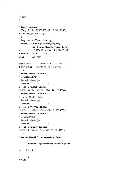
第七章1.a.> lamp<-data.frame(+ X=c(115,116,98,83,103,107,118,116,73,89,85,97),+ A=factor(rep(1:3,c(4,4,4)))+ )> lamp.aov<-aov(X ~ A, data=lamp)> source("anova.tab.R");anova.tab(lamp.aov)Df Sum Sq Mean Sq F value Pr(>F)A 2 1304.00 652.00 4.9228 0.03595 * Residuals 9 1192.00 132.44Total 11 2496.00---Signif. codes: 0 ‘***’ 0.001 ‘**’ 0.01 ‘*’ 0.05 ‘.’ 0.1 ‘.’ 1 P值大于0.01,接受原假设。
没有显著差异b.> source("interval_estimatel.R")> x<-c(115,116,98,83)> interval_estimatel(x)mean df a b1 103 3 78.04264 127.9574均值为103,区间估计为(78.04264,127.9574)> source("interval_estimatel.R")> x<-c(103,107,118,116)> interval_estimatel(x)mean df a b1 111 3 99.59932 122.4007均值为111,区间估计为(99.59932,122.4007)> source("interval_estimatel.R")> x<-c(73,89,85,97)> interval_estimatel(x)mean df a b186 3 70.08777 101.9122均值为86,区间估计为(70.08777,101.9122)c.> pairwise.t.test(X, A, p.adjust.method = "none")Pairwise comparisons using t tests with pooled SD data: X and A1 22 0.351 -3 0.066 0.013> X=c(115,116,98,83,103,107,118,116,73,89,85,97)> A=factor(rep(1:3,c(4,4,4)))> pairwise.t.test(X, A, p.adjust.method = "holm")Pairwise comparisons using t tests with pooled SDdata: X and A1 22 0.35 -3 0.13 0.04P value adjustment method: holm> X=c(115,116,98,83,103,107,118,116,73,89,85,97)> A=factor(rep(1:3,c(4,4,4)))> pairwise.t.test(X, A, p.adjust.method = "bonferroni")Pairwise comparisons using t tests with pooled SDdata: X and A1 22 1.00 -3 0.20 0.04P value adjustment method: bonferroni2.> lamp<-data.frame(+ X=c(20,18,18,17,15,16,13,18,22,17,26,19,26,28,23,25,24,25,18,22,27,24,12,14), + A=factor(rep(1:4,c(10,6,6,2)))+ )> lamp.aov<-aov(X ~ A, data=lamp)> source("anova.tab.R");anova.tab(lamp.aov)Df Sum Sq Mean Sq F value Pr(>F)A 3 351.72 117.24 15.105 2.277e-05 ***Residuals 20 155.23 7.76Total 23 506.96---Signif. codes: 0 ‘***’ 0.001 ‘**’ 0.01 ‘*’ 0.05 ‘.’ 0.1 ‘ ’ 1p值远远小于0.01,拒绝原假设。

统计建模与r软件课后习题答案统计建模与R软件课后习题答案在统计建模与R软件课程中,学生们经常需要完成一系列的习题来巩固所学知识。
这些习题涉及到统计建模的理论和实践,以及如何使用R软件来进行数据分析和建模。
在本文中,我们将给出一些常见的统计建模与R软件课后习题的答案,希望能够帮助学生更好地理解课程内容。
1. 线性回归模型习题:使用R软件对给定数据集进行线性回归分析,并给出回归方程和相关系数。
答案:在R软件中,可以使用lm()函数来进行线性回归分析。
例如,对于数据集data,可以使用以下代码进行线性回归分析:```model <- lm(y ~ x, data=data)summary(model)```其中,y和x分别表示因变量和自变量。
通过summary()函数可以得到回归方程和相关系数等信息。
2. 逻辑回归模型习题:使用R软件对给定数据集进行逻辑回归分析,并给出回归方程和模型拟合度。
答案:逻辑回归分析可以使用glm()函数来进行。
例如,对于数据集data,可以使用以下代码进行逻辑回归分析:```model <- glm(y ~ x, data=data, family=binomial)summary(model)```其中,y和x分别表示因变量和自变量,family=binomial表示使用二项分布进行逻辑回归分析。
通过summary()函数可以得到回归方程和模型拟合度等信息。
3. 方差分析习题:使用R软件对给定数据集进行方差分析,并给出各组之间的差异是否显著。
答案:在R软件中,可以使用aov()函数来进行方差分析。
例如,对于数据集data,可以使用以下代码进行方差分析:```model <- aov(y ~ group, data=data)summary(model)```其中,y和group分别表示因变量和自变量。
通过summary()函数可以得到各组之间的差异是否显著等信息。

软件建模与UML智慧树知到课后章节答案2023年下山东理工大学山东理工大学第一章测试1.结构化设计阶段的主要设计思路是()。
答案:自顶向下,逐步求精2.结构化分析建模的3种核心模型为()。
答案:DD;ERD;DFD3.数据流图的外部实体可能是与系统交互的()。
答案:硬件设备;人;软件系统;部门;组织4.环境图也称顶层数据流图,它仅包括一个数据处理过程,即目标系统。
答案:对5.ER图是数据库设计的基础,因此又称为()。
答案:数据库概念模型6.数据字典是以词条方式定义在数据模型、功能模型和行为模型中出现的数据对象及控制信息的特性,其定义对象包括()。
答案:数据源点/汇点;加工(过程)条目;数据流条目;数据文件7.DD中最常用的数据结构描述方式有()。
答案:定义式 ;Warier图8.结构图可以清楚的表达出模块间的层次调用关系和信息传递,但不能表达有条件的模块调用。
答案:错9.结构图优化时,需要应用高耦合、低内聚原则。
答案:错10.关于结构化程序设计的描述,正确的是()。
答案:选用的控制结构只准有一个入口和一个出口。
; 使用顺序、选择、循环这三种基本控制结构表达程序逻辑。
; 严格控制GOTO语句。
11.请根据描述,对学校图书管理系统建立DFD。
图书管理系统主要目的是方便学校图书馆的借还书工作。
图书管理员负责进行图书的管理,主要包括图书的入库、图书信息的修改和图书的出库。
其他工作人员负责完成借书和还书的操作。
读者可以通过系统查询图书信息及流通状态,可以自助借书、还书。
另外还可以通过系统进行图书的预约和续借。
读者分为教师和学生。
教师最多允许借10本书,借阅时长2个月。
学生最多允许借5本书,借阅时长为1个月。
两类读者的续借时长都为1个月。
对已借出图书到期时长小于一周时,允许预约,预约期为10天,多位读者预约时,按预约时间排序;超期未借,预约自动失效。
存在预约的图书只能由预约读者借阅。
还书时,如果发生超期,需要缴纳罚款。
文档来源为:从网络收集整理.word版本可编辑.欢迎下载支持.第六章、单项选择题1.下面的函数关系是()A现代化水平与劳动生产率圆周的长度决定于它的半径C家庭的收入和消费的关系亩产量与施肥量2.相关系数r的取值范围B -1C -1< r < +13.年劳动生产率x(干元)和工人工资y=10+70x,这意味着年劳动生产率每提高1千元时,工人工资平均()A增加70元 B 减少70元C增加80元D减少80元4.若要证明两变量之间线性相关程度高, 则计算出的相关系数应接近于A +1B -1C 0.5 D5.回归系数和相关系数的符号是一致的, 其符号均可用来判断现象A线性相关还是非线性相关 B 正相关还是负相关C完全相关还是不完全相关 D 单相关还是复相关6.某校经济管理类的学生学习统计学的时间(X)与考试成绩(y)之间建立线性回归方程? =a+bx。
经计算,方程为? =200— 0.8X,该方程参数的计算()Aa值是明显不对的值是明显不对的C a值和b值都是不对的D a 值和b值都是正确的7.在线性相关的条件下, 自变量的均方差为2,因变量均方差为5,而相关系数为0.8 时,则其回归系数为:()A 8B 0.32C 2D 12&进行相关分析,要求相关的两个变量A都是随机的C一个是随机的,一个不是随机的随机或不随机都可以都不是随机的9.下列关系中,属于正相关关系的有A合理限度内,施肥量和平均单产量之间的关系B产品产量与单位产品成本之间的关系C商品的流通费用与销售利润之间的关系D流通费用率与商品销售量之间的关系10.相关分析是研究 ( )A变量之间的数量关系变量之间的变动关系C变量之间的相互关系的密切程度 D 变量之间的因果关系11.在回归直线 y c=a+bx ,b<0,则x与y之间的相关系数()A r=0B r=lC 0< r<1D -1< r <012.当相关系数 r=0 时,表明 (A现象之间完全无关 B 相关程度较小C现象之间完全相关 D 无直线相关关系13.下列现象的相关密切程度最高的是 ( )A某商店的职工人数与商品销售额之间的相关系数0.87B流通费用水平与利润率之间的相关系数为-0.94C商品销售额与利润率之间的相关系数为0.51D商品销售额与流通费用水平的相关系数为-0.8114.估计标准误差是反映 ( )A平均数代表性的指标相关关系的指标C回归直线方程的代表性指标D序时平均数代表性指标二、多项选择题1.下列哪些现象之间的关系为相关关系( )A 家庭收入与消费支出关系B 圆的面积与它的半径关系C广告支出与商品销售额关系D商品价格一定,商品销售与额商品销售量关系2.相关系数表明两个变量之间的( )A因果关系 C变异程度 D 相关方向 E 相关的密切程度3.对于一元线性回归分析来说( )A两变量之间必须明确哪个是自变量,哪个是因变量B回归方程是据以利用自变量的给定值来估计和预测因变量的平均可能值C 可能存在着 y 依 x 和 x 依 y 的两个回归方程D回归系数只有正号4.可用来判断现象线性相关方向的指标有( )A相关系数 B 回归系数 C 回归方程参数a D 估计标准误5.单位成本 ( 元)依产量 (千件 )变化的回归方程为 y c=78- 2x ,这表示 ( ) A产量为1000件时,单位成本 76元B产量为1000件时,单位成本 78元C产量每增加1000件时,单位成本下降 2元D产量每增加1000件时,单位成本下降 78元6.估计标准误的作用是表明 ( )A样本的变异程度回归方程的代表性C估计值与实际值的平均误差D样本指标的代表性7.销售额与流通费用率,在一定条件下,存在相关关系,这种相关关系属于A完全相关 B 单相关 C 负相关 D 复相关8.在直线相关和回归分析中 ( )A据同一资料, 相关系数只能计算一个B据同一资料, 相关系数可以计算两个C据同一资料, 回归方程只能配合一个D据同一资料, 回归方程随自变量与因变量的确定不同,可能配合两个9.相关系数 r 的数值 ( )A可为正值 B 可为负值 C 可大于1 D 可等于-110.从变量之间相互关系的表现形式看,相关关系可分为A正相关 B 负相关 C直线相关 D 曲线相关11.确定直线回归方程必须满足的条件是 ( )A现象间确实存在数量上的相互依存关系B 相关系数 r 必须等于 1C y与x必须同方向变化D现象间存在着较密切的直线相关关系12.当两个现象完全相关时,下列统计指标值可能为A r=1B r=0C r=-1D S y=013.在直线回归分析中,确定直线回归方程的两个变量必须是A一个自变量,一个因变量均为随机变量C对等关系一个是随机变量,一个是可控制变量14.配合直线回归方程是为了A确定两个变量之间的变动关系用因变量推算自变量C用自变量推算因变量两个变量都是随机的15.在直线回归方程中 ( )A在两个变量中须确定自变量和因变量 B 一个回归方程只能作一种推算C要求自变量是给定的,而因变量是随机的。
第二章2.1> x<-c(1,2,3);y<-c(4,5,6)> e<-c(1,1,1)> z<-2*x+y+e;z[1] 7 10 13>z1<-crossprod(x,y);z1[,1][1,] 32>z2<-outer(x,y);z2[,1] [,2] [,3][1,] 4 5 6[2,] 8 10 12[3,] 12 15 182.2(1) > A<-matrix(1:20,nrow=4);B<-matrix(1:20,nrow=4,byrow=T) >C<-A+B;C(2) > D<-A%*%B;D(3) > E<-A*B;E(4) > F<-A[1:3,1:3](5) > G<-B[,-3]2.3>x<-c(rep(1,5),rep(2,3),rep(3,4),rep(4,2));x2.4>H<-matrix(nrow=5,ncol=5)>for (i in 1:5)+ for(j in 1:5)+ H[i,j]<-1/(i+j-1)(1)> det(H)(2)> solve(H)(3)> eigen(H)2.5>studentdata<-data.frame(姓名=c('张三','李四','王五','赵六','丁一') + ,性别=c('女','男','女','男','女'),年龄=c('14','15','16','14','15'),+ 身高=c('156','165','157','162','159'),体重=c('42','49','41.5','52','45.5')) 2.6>write.table(studentdata,file='student.txt')>write.csv(studentdata,file='student.csv')2.7count<-function(n){if (n<=0)print('要求输入一个正整数')else{ repeat{if (n%%2==0)n<-n/2elsen<-(3*n+1)if(n==1)break}print('运算成功')}}第三章3.1首先将数据录入为x。
第二章答案:Ex2.1x<-c(1,2,3)y<-c(4,5,6)e<-c(1,1,1)z=2*x+y+ez1=crossprod(x,y)#z1为x1与x2的内积或者x%*%yz2=tcrossprod(x,y)#z1为x1与x2的外积或者x%o%yz;z1;z2要点:基本的列表赋值方法,内积和外积概念。
内积为标量,外积为矩阵。
Ex2.2A<-matrix(1:20,c(4,5));AB<-matrix(1:20,nrow=4,byrow=TRUE);BC=A+B;C#不存在AB这种写法E=A*B;EF<-A[1:3,1:3];FH<-matrix(c(1,2,4,5),nrow=1);H#H起过渡作用,不规则的数组下标G<-B[,H];G要点:矩阵赋值方法。
默认是byrow=FALSE,数据按列放置。
取出部分数据的方法。
可以用数组作为数组的下标取出数组元素。
Ex2.3x<-c(rep(1,times=5),rep(2,times=3),rep(3,times=4),rep(4,times=2));x #或者省略times=,如下面的形式x<-c(rep(1,5),rep(2,3),rep(3,4),rep(4,2));x要点:rep()的使用方法。
rep(a,b)即将a重复b次Ex2.4n <- 5; H<-array(0,dim=c(n,n))for (i in 1:n){for (j in 1:n){H[i,j]<-1/(i+j-1)}};HG <- solve(H);G #求H的逆矩阵ev <- eigen(H);ev #求H的特征值和特征向量要点:数组初始化;for循环的使用待解决:如何将很长的命令(如for循环)用几行打出来再执行?每次想换行的时候一按回车就执行了还没打完的命令...Ex2.5StudentData<-data.frame(name=c("zhangsan","lisi","wangwu","zhaoliu","dingyi"),sex=c("F","M", "F","M","F"),age=c("14","15","16","14","15"),height=c("156","165","157","162","159"),weight=c( "42","49","41.5","52","45.5"));StudentData要点:数据框的使用待解决:SSH登陆linux服务器中文显示乱码。
统计建模与R软件课后答案文档编制序号:[KKIDT-LLE0828-LLETD298-POI08]第二章> x<-c(1,2,3);y<-c(4,5,6)> e<-c(1,1,1)> z<-2*x+y+e;z[1] 7 10 13> z1<-crossprod(x,y);z1[,1][1,] 32> z2<-outer(x,y);z2[,1] [,2] [,3][1,] 4 5 6[2,] 8 10 12[3,] 12 15 18(1) > A<-matrix(1:20,nrow=4);B<-matrix(1:20,nrow=4,byrow=T) > C<-A+B;C(2)> D<-A%*%B;D(3)> E<-A*B;E(4)> F<-A[1:3,1:3](5)> G<-B[,-3]> x<-c(rep(1,5),rep(2,3),rep(3,4),rep(4,2));x> H<-matrix(nrow=5,ncol=5)> for (i in 1:5)+ for(j in 1:5)+ H[i,j]<-1/(i+j-1)(1)> det(H)(2)> solve(H)(3)> eigen(H)> studentdata<(姓名=c('张三','李四','王五','赵六','丁一')+ ,性别=c('女','男','女','男','女'),年龄=c('14','15','16','14','15'), + 身高=c('156','165','157','162','159'),体重=c('42','49','','52',''))> (studentdata,file='')> (studentdata,file='')count<-function(n){if (n<=0)print('要求输入一个正整数')else{repeat{if (n%%2==0)n<-n/2elsen<-(3*n+1)if(n==1)break}print('运算成功')}}第三章首先将数据录入为x。
Homework6.4 P332解:这个过程中回归R语言计算过程如下:toothpaste<-data.frame(X1<-c(-0.05,0.25,0.60,0,0.25,0.2,0.15,0.05,-0.15,0.15,0.2,0.1,0.4,0.45,0.35,0.3,0.5,0.5,0.4,-0.05,-0 .05,-0.1,0.2,0.1,0.5,0.6,-0.05,0,0.05,0.55),X2<-c(5.5,6.75,7.25,5.5,7,6.5,6.75,5.25,5.25,6,6.5,6.25,7,6.9,6.8,6.8,7.1,7,6.8,6.5,6.25,6,6.5,7,6.8, 6.8,6.5,5.75,5.8,6.8),Y<-c(7.38,8.51,9.52,7.5,9.33,8.28,8.75,7.87,7.1,8,7.89,8.15,9.1,8.86,8.9,8.87,9.26,9,8.75,7.95,7.6 5,7.27,8,8.5,8.75,9.21,8.27,7.67,7.93,9.26))lm.sol<-lm(Y~X1+X2,data=toothpaste);summary(lm.sol)influence.measures(lm.sol)回归结果输出如下:Call:lm(formula = Y ~ X1 + X2, data = toothpaste)Residuals:Min 1Q Median 3Q Max-0.49779 -0.12031 -0.00867 0.11084 0.58106Coefficients:Estimate Std. Error t value Pr(>|t|)(Intercept) 4.4075 0.7223 6.102 1.62e-06 ***X1 1.5883 0.2994 5.304 1.35e-05 ***X2 0.5635 0.1191 4.733 6.25e-05 ***---Signif. codes: 0 '***' 0.001 '**' 0.01 '*' 0.05 '.' 0.1 ' ' 1Residual standard error: 0.2383 on 27 degrees of freedomMultiple R-squared: 0.886, Adjusted R-squared: 0.8776F-statistic: 105 on 2 and 27 DF, p-value: 1.845e-13从上述输出的结果知道,模型通过t检验和F检验,因此可以得到回归模型:.4XXY++=407556352.015883.1回归诊断结果如下:Influence measures oflm(formula = Y ~ X1 + X2, data = toothpaste) :dfb.1_ dfb.X1 dfb.X2 dffit cov.r cook.d hat inf1 -0.05536 -6.96e-03 0.050306 -0.0807 1.281 2.25e-03 0.13012 0.04401 2.83e-02 -0.048123 -0.0922 1.152 2.92e-03 0.04703 -0.01269 6.49e-02 0.010195 0.1295 1.277 5.78e-03 0.13394 -0.00929 -2.98e-03 0.008653 -0.0118 1.299 4.81e-05 0.13805 -0.68922 -4.88e-01 0.719765 0.9115 0.536 2.18e-01 0.0909 *6 0.01121 1.59e-02 -0.016637 -0.0860 1.133 2.54e-03 0.03487 -0.26976 -2.67e-01 0.290196 0.3922 0.997 4.98e-02 0.07968 1.17309 6.39e-01 -1.129656 1.2670 0.895 4.69e-01 0.2493 *9 -0.03920 -5.27e-05 0.035418 -0.0601 1.373 1.25e-03 0.1860 *10 -0.02101 -1.08e-02 0.019442 -0.0295 1.194 3.02e-04 0.063611 0.05653 8.02e-02 -0.083875 -0.4338 0.670 5.42e-02 0.034812 0.00259 -1.74e-02 0.001766 0.0546 1.160 1.03e-03 0.041913 -0.04609 1.35e-02 0.047372 0.1279 1.167 5.61e-03 0.065614 -0.00181 -8.57e-02 0.001894 -0.1784 1.149 1.08e-02 0.070715 -0.01729 1.83e-02 0.019442 0.0994 1.149 3.39e-03 0.047616 -0.05590 -1.53e-02 0.060772 0.1449 1.118 7.15e-03 0.046517 -0.01349 3.00e-02 0.012894 0.0786 1.223 2.13e-03 0.090618 0.00123 -1.01e-01 0.000402 -0.1972 1.173 1.33e-02 0.088119 -0.00397 -5.62e-02 0.002754 -0.1299 1.149 5.78e-03 0.056620 0.04972 6.92e-02 -0.054542 -0.0782 1.320 2.11e-03 0.155121 0.11714 2.36e-01 -0.139343 -0.2970 1.142 2.97e-02 0.102022 0.08114 3.85e-01 -0.126203 -0.5601 0.929 9.84e-02 0.104123 0.04240 6.02e-02 -0.062902 -0.3253 0.841 3.29e-02 0.034824 0.01971 1.90e-02 -0.020667 -0.0235 1.378 1.90e-04 0.1873 *25 -0.13024 -3.05e-01 0.133977 -0.4177 1.038 5.69e-02 0.098226 0.01670 3.14e-02 -0.017393 0.0367 1.351 4.67e-04 0.1714 *27 -0.35156 -4.89e-01 0.385694 0.5528 1.100 9.94e-02 0.155128 0.01703 -1.01e-04 -0.014952 0.0296 1.223 3.03e-04 0.085529 0.14921 3.39e-02 -0.134903 0.2241 1.140 1.70e-02 0.080230 0.10055 2.05e-01 -0.104290 0.2545 1.227 2.21e-02 0.1309从上面诊断输出结果可以得到对回归模型存在影响的有样本点5、8、9、24、26,从dfb.1_角度看,点8对响应变量影响最大,从dffit cov.r 角度看,点24、26对自变量影响最大,那么考虑去掉样本点8、24、26除去影响点后整个R语言的计算过程如下:toothpaste<-data.frame( X1=c(-0.05,0.25,0.60,0,0.20,0.15,-0.15,0.15,0.10,0.40,0.45,0.35,0.30,0.5 0,0.50,0.40,-0.05,-0.05,-0.10,0.20,0.10,0.50,0.60,-0.05,0,0.05,0.55),X2=c(5.50,6.75,7.25,5.50,6.50,6.75,5.25,6.00,6.25,7.00,6.90,6.80,6.80,7.10,7.00,6.80,6.50,6.25,6. 00,6.50,7.00,6.80,6.80,6.50,5.75,5.80,6.80),Y=c(7.38,8.51,9.52,7.50,8.28,8.75,7.10,8.00,8.15,9.10,8.86,8.90,8.87,9.26,9.00,8.75,7.95,7.65,7.27,8.00,8.50,8.75,9.21,8.27,7.67,7.93,9.26))lm.sol<-lm(Y~X1+X2,data=toothpaste);summary(lm.sol)回归输出结果如下:Call:lm(formula = Y ~ X1 + X2, data = toothpaste)Residuals:Min 1Q Median 3Q Max-0.37130 -0.10114 0.03066 0.10016 0.30162Coefficients:Estimate Std. Error t value Pr(>|t|)(Intercept) 4.0759 0.6267 6.504 1.00e-06 ***X1 1.5276 0.2354 6.489 1.04e-06 ***X2 0.6138 0.1027 5.974 3.63e-06 ***---Signif. codes: 0 '***' 0.001 '**' 0.01 '*' 0.05 '.' 0.1 ' ' 1Residual standard error: 0.1767 on 24 degrees of freedomMultiple R-squared: 0.9378, Adjusted R-squared: 0.9327F-statistic: 181 on 2 and 24 DF, p-value: 3.33e-15模型通过t 检验和F 检验,因此回归模型为:26138.015276.10759.4X X Y ++=∧。
第六章 1. a .> x <- c(5.1, 3.5, 7.1, 6.2, 8.8, 7.8, 4.5, 5.6, 8.0, 6.4)> y <- c(1907, 1287, 2700, 2373, 3260, 3000, 1947, 2273, 3113,2493) > plot(x,y)456789150020002500300xyX 与Y 线性相关b .> x <- c(5.1, 3.5, 7.1, 6.2, 8.8, 7.8, 4.5, 5.6, 8.0, 6.4)> y <- c(1907, 1287, 2700, 2373, 3260, 3000, 1947, 2273, 3113,2493) > lm.sol<-lm(y~1+x) > summary(lm.sol) Call:lm(formula = y ~ 1 + x)Residuals:Min 1Q Median 3Q Max-128.591 -70.978 -3.727 49.263 167.228Coefficients:Estimate Std. Error t value Pr(>|t|)(Intercept) 140.95 125.11 1.127 0.293x 364.18 19.26 18.908 6.33e-08 ***---Signif. codes: 0 ‘***’ 0.001 ‘**’ 0.01 ‘*’ 0.05 ‘.’ 0.1 ‘ ’ 1Residual standard error: 96.42 on 8 degrees of freedomMultiple R-Squared: 0.9781, Adjusted R-squared: 0.9754F-statistic: 357.5 on 1 and 8 DF, p-value: 6.33e-08回归方程为Y=140.95+364.18X,极为显著d.> new <- data.frame(x=7)> lm.pred <- predict(lm.sol,new,interval="prediction",level=0.95)> lm.predfit lwr upr[1,] 2690.227 2454.971 2925.484Y(7)= 2690.227, [2454.971,2925.484]2.> out<-data.frame(+ x1 <- c(0.4,0.4,3.1,0.6,4.7,1.7,9.4,10.1,11.6,12.6,10.9,23.1,23.1,21.6,23.1,1.9,26.8,29.9), + x2 <- c(52,34,19,34,24,65,44,31,29,58,37,46,50,44,56,36,58,51),+ x3 <- c(158,163,37,157,59,123,46,117,173,112,111,114,134,73,168,143,202,124),+ y <- c(64,60,71,61,54,77,81,93,93,51,76,96,77,93,95,54,168,99)+ )> lm.sol<-lm(y~x1+x2+x3,data=out)> summary(lm.sol)Call:lm(formula = y ~ x1 + x2 + x3, data = out)Residuals:Min 1Q Median 3Q Max-27.575 -11.160 -2.799 11.574 48.808Coefficients:Estimate Std. Error t value Pr(>|t|)(Intercept) 44.9290 18.3408 2.450 0.02806 *x1 1.8033 0.5290 3.409 0.00424 **x2 -0.1337 0.4440 -0.301 0.76771x3 0.1668 0.1141 1.462 0.16573---Signif. codes: 0 ‘***’ 0.001 ‘**’ 0.01 ‘*’ 0.05 ‘.’ 0.1 ‘ ’ 1Residual standard error: 19.93 on 14 degrees of freedomMultiple R-Squared: 0.551, Adjusted R-squared: 0.4547F-statistic: 5.726 on 3 and 14 DF, p-value: 0.009004回归方程为y=44.9290+1.8033x1-0.1337x2+0.1668x3由计算结果可以得到,回归系数与回归方程的检验都是显著的3.a.> x<-c(1,1,1,1,2,2,2,3,3,3,4,4,4,5,6,6,6,7,7,7,8,8,8,9,11,12,12,12)> y<-c(0.6,1.6,0.5,1.2,2.0,1.3,2.5,2.2,2.4,1.2,3.5,4.1,5.1,5.7,3.4,9.7,8.6,4.0,5.5,10.5,17.5,13.4,4.5, + 30.4,12.4,13.4,26.2,7.4)> lm.sol <- lm(y ~ 1+x)> summary(lm.sol)Call:lm(formula = y ~ 1 + x)Residuals:Min 1Q Median 3Q Max-9.84130 -2.33691 -0.02137 1.05921 17.83201Coefficients:Estimate Std. Error t value Pr(>|t|)(Intercept) -1.4519 1.8353 -0.791 0.436x 1.5578 0.2807 5.549 7.93e-06 ***---Signif. codes: 0 ‘***’ 0.001 ‘**’ 0.01 ‘*’ 0.05 ‘.’ 0.1 ‘ ’ 1Residual standard error: 5.168 on 26 degrees of freedomMultiple R-Squared: 0.5422, Adjusted R-squared: 0.5246F-statistic: 30.8 on 1 and 26 DF, p-value: 7.931e-06线性回归方程为y=-1.4519+1.5578x,并且未通过t检验和F检验> plot(x,y)> abline(-1.4519,1.5578)>246810120510********xyc .> x<-c(1,1,1,1,2,2,2,3,3,3,4,4,4,5,6,6,6,7,7,7,8,8,8,9,11,12,12,12)> y<-c(0.6,1.6,0.5,1.2,2.0,1.3,2.5,2.2,2.4,1.2,3.5,4.1,5.1,5.7,3.4,9.7,8.6,4.0,5.5,10.5,17.5,13.4,4.5, + 30.4,12.4,13.4,26.2,7.4)> y.res<-resid(lm.sol);y.fit<-predict(lm.sol) > plot(y.res~y.fit)> y.rst<-rstandard(lm.sol) > plot(y.rst~y.fit) >普通残差051015-10-5051015y.fity .r e s标准化残差051015-2-10123y.fity .r s td . (4)> lm.new<-update(lm.data3,sqrt(.)~.);coef(lm.new) (Intercept) x 0.7665018 0.29136202x 0.084890650.4466549x 0.58752220.2913620x0.7665018 ++=+=∧∧y y> plot(x,y)> lines(x,y=0.5875222+0.08489065*x^2+0.4466549*x) > y.res<-resid(lm.new);y.fit<-predict(lm.new) > plot(y.res~y.fit)> y.rst<-rstandard(lm.new)> plot(y.rst~y.fit)4.> lm.sol<-lm(Y~X1+X2,data=toothpaste)> summary(lm.sol)Call:lm(formula = Y ~ X1 + X2, data = toothpaste)Residuals:Min 1Q Median 3Q Max-0.497785 -0.120312 -0.008672 0.110844 0.581059Coefficients:Estimate Std. Error t value Pr(>|t|)(Intercept) 4.4075 0.7223 6.102 1.62e-06 ***X1 1.5883 0.2994 5.304 1.35e-05 ***X2 0.5635 0.1191 4.733 6.25e-05 ***---Signif. codes: 0 ‘***’ 0.001 ‘**’ 0.01 ‘*’ 0.05 ‘.’ 0.1 ‘ ’ 1Residual standard error: 0.2383 on 27 degrees of freedomMultiple R-squared: 0.886, Adjusted R-squared: 0.8776F-statistic: 105 on 2 and 27 DF, p-value: 1.845e-13> source("Reg_Diag.R");Reg_Diag(lm.sol)residual s1 standard s2 student s3 hat_matrix s4 DFFITS1 -0.047231639 -0.21248023 -0.20868284 0.13012303 -0.080711402 -0.098070223 -0.42151698 -0.41500522 0.04704358 -0.092207713 0.074288624 0.33492116 0.32934525 0.13385955 0.129473814 -0.006645926 -0.03003380 -0.02947287 0.13797634 -0.011791395 0.581059204 * 2.55701395 * 2.88236603 * 0.09091719 0.911528866 -0.107785364 -0.46031439 -0.45349258 0.03475104 -0.086046747 0.300758350 1.31532456 1.33418993 0.07955382 0.392237398 0.424810360 2.05723960 * 2.19842345 * 0.24932956 * 1.266991129 -0.027532493 -0.12804079 -0.12568545 0.18600211 -0.0600803310 -0.026629932 -0.11546376 -0.11333335 0.06356511 -0.0295276111 -0.497785364 -2.12587089 * -2.28622467 * 0.03475104 -0.4337935912 0.061913782 0.26540305 0.26078220 0.04194215 0.0545641513 0.112816344 0.48968055 0.48267493 0.06556908 0.1278588114 -0.150249714 -0.65395500 -0.64687388 0.07069034 -0.1784101015 0.104927089 0.45112292 0.44436784 0.04761107 0.0993549316 0.154341375 0.66319490 0.65616401 0.04652075 0.1449372917 0.057639541 0.25360011 0.24915642 0.09056633 0.0786266818 -0.146012230 -0.64156026 -0.63442169 0.08813106 -0.1972315219 -0.124487198 -0.53776150 -0.53055795 0.05659354 -0.1299471720 -0.040713930 -0.18584177 -0.18248454 0.15505538 -0.0781727521 -0.199843357 -0.88485598 -0.88118586 0.10202733 -0.2970258322 -0.359558498 -1.59386063 -1.64328265 0.10408399 -0.5601064823 -0.387785364 -1.65609855 -1.71455446 0.03475104 -0.3253235524 -0.010697936 -0.04979066 -0.04886215 0.18729463 -0.0234568025 -0.283315771 -1.25181018 -1.26568782 0.09823492 -0.4177465226 0.017855655 0.08230563 0.08077720 0.17144488 0.0367443327 0.279286070 1.27482211 1.29043074 0.15505538 0.5527948628 0.022483501 0.09864705 0.09682047 0.08548985 0.0296026229 0.174895100 0.76513625 0.75910825 0.08017207 0.2241103830 0.147269942 0.66281470 0.65578162 0.13089383 0.25449685s5 cooks_distance s6 COVRATIO s71 2.251190e-03 1.28095242 2.923723e-03 1.15211573 5.778631e-03 1.27690564 4.812656e-05 1.29899825 * 2.179654e-01 0.5361673 *6 2.542824e-03 1.13309647 4.984335e-02 0.99745488 * 4.685683e-01 * 0.89452379 1.248734e-03 1.373272210 3.016556e-04 1.194126111 5.423517e-02 0.669681912 1.027897e-03 1.159781213 5.608624e-03 1.166813514 1.084362e-02 1.148706415 3.391268e-03 1.149474316 7.153137e-03 1.118050417 2.134879e-03 1.222624518 1.326021e-02 1.172800619 5.782640e-03 1.149323820 2.112633e-03 1.320308321 2.965359e-02 1.141740222 9.837757e-02 0.929311223 3.291392e-02 0.841337024 1.904437e-04 1.377585325 5.690208e-02 1.037953426 4.672410e-04 1.350588127 9.941147e-02 1.100173228 3.032306e-04 1.223243929 1.700877e-02 1.139997330 2.205512e-02 1.2266609> toothpaste<-data.frame(+ X1=c(-0.05, 0.25,0.60,0,0.20, 0.15,-0.15, 0.15,+ 0.10,0.40,0.45,0.35,0.30, 0.50,0.50, 0.40,-0.05,+ -0.05,-0.10,0.20,0.10,0.50,0.60,-0.05,0, 0.05, 0.55), + X2=c( 5.50,6.75,7.25,5.50,6.50,6.75,5.25,6.00,+ 6.25,7.00,6.90,6.80,6.80,7.10,7.00,6.80,6.50,+ 6.25,6.00,6.50,7.00,6.80,6.80,6.50,5.75,5.80,6.80), + Y =c( 7.38,8.51,9.52,7.50,8.28,8.75,7.10,8.00,+ 8.15,9.10,8.86,8.90,8.87,9.26,9.00,8.75,7.95,+ 7.65,7.27,8.00,8.50,8.75,9.21,8.27,7.67,7.93,9.26) + )>> lm.sol<-lm(Y~X1+X2,data=toothpaste)> summary(lm.sol)Call:lm(formula = Y ~ X1 + X2, data = toothpaste)Residuals:Min 1Q Median 3Q Max-0.37130 -0.10114 0.03066 0.10016 0.30162Coefficients:Estimate Std. Error t value Pr(>|t|) (Intercept) 4.0759 0.6267 6.504 1.00e-06 ***X1 1.5276 0.2354 6.489 1.04e-06 ***X2 0.6138 0.1027 5.974 3.63e-06 ***---Signif. codes: 0 ‘***’ 0.001 ‘**’ 0.01 ‘*’ 0.05 ‘.’ 0.1 ‘ ’ 1Residual standard error: 0.1767 on 24 degrees of freedom Multiple R-squared: 0.9378, Adjusted R-squared: 0.9327F-statistic: 181 on 2 and 24 DF, p-value: 3.33e-155.XX<-cor(cement[1:4])kappa(XX,exact=TRUE)[1] 1376.881> eigen(XX)$values[1] 2.235704035 1.576066070 0.186606149 0.001623746$vectors[,1] [,2] [,3] [,4][1,] -0.4759552 0.5089794 0.6755002 0.2410522[2,] -0.5638702 -0.4139315 -0.3144204 0.6417561[3,] 0.3940665 -0.6049691 0.6376911 0.2684661[4,] 0.5479312 0.4512351 -0.1954210 0.6767340删去了X3,X4> cement<-data.frame(+ X1=c( 7, 1, 11, 11, 7, 11, 3, 1, 2, 21, 1, 11, 10),+ X2=c(26, 29, 56, 31, 52, 55, 71, 31, 54, 47, 40, 66, 68),+ Y =c(78.5, 74.3, 104.3, 87.6, 95.9, 109.2, 102.7, 72.5, + 93.1,115.9, 83.8, 113.3, 109.4)+ )> XX<-cor(cement[1:2])> kappa(XX,exact=TRUE)[1] 1.592620复共线性消失了。