Oracle Performance Management on major Operating Systems WULZ- A walk in the park or a wulz

Oracle® Enterprise Manager Ops CenterMonitor and Manage Incidents Workflow12c Release 1 (12.1.2.0.0)E37388-01November 2012This workflow provides an end-to-end example for how to use Oracle EnterpriseManager Ops Center.IntroductionWorkflows are divided into two categories: Deploy and Operate. Each workflow is acompilation of several examples.This workflow is an example of how to use Oracle Enterprise Manager Ops Center tomonitor and manage the deployed hardware and operating systems.Oracle Enterprise Manager Ops Center can detect when a managed asset does notoperate within the specified parameters. You can define the polices for monitoring theasset. An asset can be a hardware, operating system, group of servers or operatingsystems, network, or a storage resource managed by Oracle Enterprise Manager OpsCenter.You can define the monitoring rules and policies for an asset. The monitoring rulesstate the values and boundaries for an asset’s activity. The set of rules is a monitoringpolicy. When you apply a monitoring policy to all the assets, it enforces consistency.When the set thresholds are exceeded, that is the asset is not performing within thedefined parameters in the monitoring rules and policies, Oracle Enterprise ManagerOps Center generates an alert and an incident.When an incident appears, you can assign it to a user for resolution and useannotations to add comments and suggested actions. You can build an IncidentKnowledge Base that contains your annotations from specific incidents, or addsuggested fixes or automated fixes for a specific type of incident.Required Permissions and RolesThe following permissions and roles the required to complete the tasks in theworkflow:■Asset AdminDiscover hardware and operating systems■Fault AdminManage the incidents to assign and take action■Plan/Profile AdminCreate and manage the profiles and plans■Ops Center AdminManage the service requests.WorkflowTo perform the operations in this workflow, Oracle Enterprise Manager Ops Center must manage the assets. The incident management is automatically enabled for an asset that is discovered and managed in Oracle Enterprise Manager Ops Center.This workflow describes how to set your monitoring policies, manage incidents, and use Service Requests in Oracle Enterprise Manager Ops Center.Figure 1Monitor and Manage Incidents WorkflowWhat’s Next?You can either follow to update the operating system managed in the Oracle Enterprise Manager Ops Center. For more information about Oracle Enterprise Manager Ops Center, refer to Oracle Enterprise Manager Ops Center Feature Reference Guide.Related Resources and ArticlesThe Oracle Enterprise Manager Ops Center 12c documentation is located at/pls/topic/lookup?ctx=oc121.See the following guides for more information:■Oracle Enterprise Manager Ops Center Feature Reference Guide for information about logical domains and server pools.■Oracle Enterprise Manager Ops Center Administration Guide for information about user roles and permissions.Other examples are available at /cd/E27363_01/nav/howto.htm.Documentation AccessibilityFor information about Oracle's commitment to accessibility, visit the Oracle Accessibility Program website at/pls/topic/lookup?ctx=acc&id=docacc.Access to Oracle SupportOracle customers have access to electronic support through My Oracle Support. For information, visit /pls/topic/lookup?ctx=acc&id=info or visit /pls/topic/lookup?ctx=acc&id=trs if you are hearing impaired.Oracle Enterprise Manager Ops Center Monitor and Manage Incidents Workflow, 12c Release 1 (12.1.2.0.0)E37388-01Copyright © 2007, 2012, Oracle and/or its affiliates. All rights reserved.This software and related documentation are provided under a license agreement containing restrictions on use and disclosure and are protected by intellectual property laws. Except as expressly permitted in your license agreement or allowed by law, you may not use, copy, reproduce, translate, broadcast, modify, license, transmit, distribute, exhibit, perform, publish, or display any part, in any form, or by any means. Reverse engineering, disassembly, or decompilation of this software, unless required by law for interoperability, is prohibited.The information contained herein is subject to change without notice and is not warranted to be error-free. If you find any errors, please report them to us in writing.If this is software or related documentation that is delivered to the U.S. Government or anyone licensing it on behalf of the U.S. Government, the following notice is applicable:U.S. GOVERNMENT END USERS: Oracle programs, including any operating system, integrated software, any programs installed on the hardware, and/or documentation, delivered to U.S. Government end users are "commercial computer software" pursuant to the applicable Federal Acquisition Regulation and agency-specific supplemental regulations. As such, use, duplication, disclosure, modification, and adaptation of the programs, including any operating system, integrated software, any programs installed on the hardware, and/or documentation, shall be subject to license terms and license restrictions applicable to the programs. No other rights are granted to the U.S. Government.This software or hardware is developed for general use in a variety of information management applications. It is not developed or intended for use in any inherently dangerous applications, including applications that may create a risk of personal injury. If you use this software or hardware in dangerous applications, then you shall be responsible to take all appropriate fail-safe, backup, redundancy, and other measures to ensure its safe use. Oracle Corporation and its affiliates disclaim any liability for any damages caused by use of this software or hardware in dangerous applications. Oracle and Java are registered trademarks of Oracle and/or its affiliates. Other names may be trademarks of their respective owners.Intel and Intel Xeon are trademarks or registered trademarks of Intel Corporation. All SPARC trademarks are used under license and are trademarks or registered trademarks of SPARC International, Inc. AMD, Opteron, the AMD logo, and the AMD Opteron logo are trademarks or registered trademarks of Advanced Micro Devices. UNIX is a registered trademark of The Open Group.This software or hardware and documentation may provide access to or information on content, products, and services from third parties. Oracle Corporation and its affiliates are not responsible for and expressly disclaim all warranties of any kind with respect to third-party content, products, and services. Oracle Corporation and its affiliates will not be responsible for any loss, costs, or damages incurred due to your access to or use of third-party content, products, or services.。

Oracle自带性能分析工具－AWR介绍和分析华三通信技术1 Oracle 10g的AWR性能优化工具简介AWR (Automatic Workload Repository)既自动工作负载信息库是Oracle10g新提供的收集数据库统计信息的置工具。

它比之前的statspack有显著的改进，收集的信息也更多、更全面，使用方法也更简单。

它主要采集与性能相关的统计数据，并从那些统计数据中导出性能量度，以跟踪潜在的问题，如包括AWR存区，历史数据存储文件和ASH等部件。

AWR报告的容繁多，官方文档也没有对所有参数给出说明。

AWR产生的报表包括以下几部分。

报表具体容参见如下插入的对象。

1、Report SummeryCache sizesLoad profileInstance Efficiency Percentages (Target 100%)Shared Pool StatisticsTop 5 Timed Events2、RAC StatisticsGlobal Cache Load ProfileGlobal Cache Efficiency Percentages (Target local+remote 100%)Global Cache and Enqueue Services - Workload CharacteristicsGlobal Cache and Enqueue Services - Messaging Statistics3、Wait Events StatisticsTime Model StatisticsWait ClassWait EventsBackground Wait EventsOperating System StatisticsService StatisticsService Wait Class Stats4、SQL StatisticsSQL ordered by Elapsed TimeSQL ordered by CPU TimeSQL ordered by GetsSQL ordered by ReadsSQL ordered by ExecutionsSQL ordered by Parse CallsSQL ordered by Sharable Memory SQL ordered by Version CountSQL ordered by Cluster Wait Time Complete List of SQL Text5、Instance Activity StatisticsInstance Activity StatsInstance Activity Stats - Absolute Values Instance Activity Stats - Thread Activity 6、IO StatsTablespace IO StatsFile IO Stats7、Buffer Pool Statistics8、Advisory StatisticsInstance Recovery StatsBuffer Pool AdvisoryPGA Aggr SummaryPGA Aggr Target StatsPGA Aggr Target HistogramPGA Memory AdvisoryShared Pool AdvisorySGA Target AdvisoryStreams Pool AdvisoryJava Pool Advisory9、Wait StatisticsBuffer Wait StatisticsEnqueue Activity10、Undo StatisticsUndo Segment SummaryUndo Segment Stats11、Latch StatisticsLatch ActivityLatch Sleep BreakdownLatch Miss SourcesParent Latch StatisticsChild Latch Statistics12、Segment StatisticsSegments by Logical ReadsSegments by Physical ReadsSegments by Row Lock WaitsSegments by ITL WaitsSegments by Buffer Busy WaitsSegments by Global Cache Buffer Busy Segments by CR Blocks ReceivedSegments by Current Blocks Received 13、Dictionary Cache StatisticsDictionary Cache StatsDictionary Cache Stats (RAC)14、Library Cache StatisticsLibrary Cache ActivityLibrary Cache Activity (RAC) 15、Memory StatisticsProcess Memory SummarySGA Memory SummarySGA breakdown difference 16、Streams StatisticsStreams CPU/IO UsageStreams CaptureStreams ApplyBuffered QueuesBuffered SubscribersRule Set17、Resource Limit Stats18、init.ora Parameters19、Global Enqueue Statistics20、Global CR Served Stats21、Global CURRENT Served Stats22、Global Cache Transfer Stats2 AWR配置2.1 AWR统计数据的缺省配置AWR 实质上是一个 Oracle 的置工具，它采集与性能相关的统计数据，并从那些统计数据中导出性能量度，以跟踪潜在的问题。

Insight GuidePayroll makesthe world go roundIt’s so obvious, we often take it for granted. That’s why Oracle Payroll’s ability to make it ‘go round’ digitally and in a timely, accurate and compliant way, is key to the successof any modern public sector organisation.StartIntroduction 3When Payroll is on a roll – everyone is happy 4What we expect from payroll – every month 5Payroll enables HR to be even more of a ‘human resource’ 6Payroll only hits the headlines when things go wrong 8Payroll designed to be human 9‘We know how to make payroll work for the UK public sector’ 12Contact 14ContentsOur contributorsSarah Wadsworth Head of HR, Fujitsu UKTracey CollinsCustomer Services Director,Government Shared Services, Fujitsu UK Eddie DavidsonHead of Oracle Payroll Delivery, Fujitsu UKorganisations you can think of– must ensure that their payroll is both highly visible and invisible at the same time.”It’s a statement that soundslike a riddle but is in fact an expression of a fundamental truth. Payroll matters because it’s how the vast majorityof us get paid each month.We take it for granted until there’s a problem. The process is invisible to all but the people who run and manage it. The money appearsin our accounts or pay packets (they do still exist) on time and ‘on the money.’ We move on.But when it doesn’t work, thenfer. “Payroll is actually a highly emotive issue,” stresses Eddie, “if your pay is wrong, or you don’t get the extra overtimeyou were expecting this monthand have to wait another, thenthat can turn your plans upsidedown.” Sarah agrees and adds;“Till then, in truth, mostemployees don’t talk to theirHR departments, and if theydo it’s a usually for functionalreasons. Payroll errors or issuesend up taking up valuable timefor both the employee andthe HR professional and canundermine the credibility ofHR itself.”And that’s what this Insight Guideis about. We’ve brought togetherthree Fujitsu experts to sharetheir experiences and opinionsabout how Oracle Payroll is thenext logical step.“It’s strange how, whenyou think about it, payrollintersects with our mostpersonal moments andlife-changing milestones.”The need to record precisely what is owed and when it should be paid was the stimulus for when a 15th century friar called Luca Pacioli decided to invent double-entry book-keeping. His carefully inked ledgers are the direct ancestors of generations of accounting and payroll methods, including21st century digital ones like Oracle Payroll. The objective has always been the same: achieve accuracy, timeliness, and compliance.Bill Monks, a public financial management expert, puts it very simply; “Payroll costs are a very government expenditures, settingaccurate and comprehensivebudgets for payroll, and ensuringefficient budget executionare critical to effective publicsector Financial Management.”1He stresses that the scrutiny onpublic finances is necessarilyintense. The money, after all,comes from our taxes (deductedby payroll!) and therefore it’svital that there is clarity andtransparency about how moneyMonks also stresses that publicsector pay is, in many countries,an engine of the wider economy.It can account for between 10%and 40% of total governmentexpenditure. That sounds a lot,but the money flows directly intoall other private businesses aswell as other public services suchas transport. A key element inKeynesian economics is, of course,to flow from government to theeconomy and back again. It’s alsoa major part of the latest iterationTheory2, which puts public sectorpay at the heart of the fightagainst inequality. Simply, whenthe public sector payroll worksbenefits. And when that happens,everyone is happy.1What we expect from payroll – every monthYes, we takepayroll for granted. That’s because it works, most of the time. But it’s complex.A definite date in the month where we can report overtime, additions, changes etc. – the later the better so they appear in the closest payslip Payroll to be to be constantlycompliant so there’s no comeback to us individually if there’s an errorAccurate payslips which reflect our contracted pay plus any overtime or additions, as well as reimbursement for expenses Transparency – a clear and simpleexplanation of all elements of our pay and deductionsNo errors – or as few errors as possiblebecause they cut the money we get, which canruin our plans and any errors that are in our ‘favour’ are just as problematic and frustratingAll deductions to be accurate – taxes, nationalinsurance, pension payments(MyCSP for the Civil Service in the UK)We expect…Payroll enables HR to be even more of a ‘human resource’Sarah Wadsworth sees payroll as the key to enabling HR teams to be more effective. “HR works when there’s trust; between the HR team and the organisation’s employees,” says Sarah, “trust gives us a mandate to engage with people on a personal level and enable them to thrive. But that mandate depends on processes that work. Payroll that pays. On time, every time.”As Sarah stressed in the introduction, payroll is the one function that intersects with our most fundamental needs and milestones: from getting that job we want to achieving the promotion we’ve worked hard for. And the other way around. “The world of work is a series of progressions and sometimes regressions which affect our pay and our sense of wellbeing,” says Sarah, “if there are errors, then that undermines the employee’s view of the entire organisation, but especially the HR department. Errors inhibit trust. And without trust HR professionals can’t use their skills.”Sarah’s focus on HR is both ‘spiritual’ and ‘functional.’ As she puts it, “You can’t get spiritual if your pay is wrong and you’re worrying about money.” That’s why a focus on the efficiency and accuracyof payroll is not something you can avoid as an HR professional. “It’s the foundation of good practice,” Sarah says.She adds, “When you can trust payroll, you can trust the people who run it, even if the person you’re talking to doesn’t run it themselves.” Digital transformation has helped HR in more agile and efficient ways. It’s delivered seamless access toan array of data which can inform both policy and practice focused on boosting employee wellbeing, engagement, and diversity of opportunity and inclusion. “HR is all about harnessing data to achieve human insights which can then inform personal engagement with employees,” says Sarah, “it’s how you can actually make the claim that you’re a ‘people business’and are using data to benefit realpeople in real work situations.”3Payroll only hits the headlines when things go wrongSearch for ‘payroll’ on the internet and it’s mostly bad news. Payroll doesn’t make headlines any other way. That’s no surprise, but the theme that recurs in all the stories is, you guessed it, error.A supermarket worker on the minimum wage in the UK thought she’d been given a pay rise when her payslips showeda higher hourly rate. She happily spent the money for a few months until she was told it was an error and she owed her employer money. She couldn’t pay. The Daily Mirror took up her caseand the employer suffered from the bad publicity.3In 2019 the National Bank of Australia announced a payroll review which finally reported in May 2021 resulting in global bad publicity. That’s because it was revealed that over 3,000 current and former employees had been paid the wrong amount and AU$55m had tobe repaid. The Finance Sector Union got involved. HR teams worked overtime to resolve the issue which was related to complex contracts and hourly rates. The fault turned out to be overly complex processes.4Payroll designed to be humanEddie Davidson sees payroll in the cloud as thebest way to make the function truly human-centric. How does Oracle Payroll enable HR to be more‘humanistic’? “When processes and tools are moved to the cloud and there’s more automation, and processes are simpler,” says Eddie, “you free up ‘human’ time and brain space. That means you deliver the payrollto keep the work turning AND you free up HR professionals to engage with and support employees.” You can also use the data that payroll provides to understand who works for you and who doesn’t,to identify gender or ethnicity pay gaps. That helps reframe employment policy and practices to attract new talent from more diverse populations. It also helps boost retention. All of which have knock-on effects both fiscally and socially. In Eddie’s view, it’s a win-win.“The public sector across the world has been moving to the cloud for the last decade,” he says, “in the UK our government’s ‘Cloud First’ policy was launched in 2013 and, despite some initial hesitancy,a lot of progress has been made. And Fujitsu has been helpinga range of departments and organisations migrate successfully.” Oracle Cloud has been centralto the projects Fujitsu has run for several government Departments totalling more than 400,000civil servants. Fujitsu therefore understands how to match the right services with the needs ofeach Department and its people.“The one thing we’re always askedall along is ‘how can we manageour payroll better?’”, says Eddie,“until now we’ve been unable tooffer them a solution that’s integralto the Oracle Cloud. But we alwaysreassured UK customers that it wascoming. And it has. It’s here.”So that’s good news? Eddiedemurs, “That depends on yourpoint of view. For me, it’s greatnews because you can now fullyintegrate what is, as we’ve stressed,a vital but complex function intothe entire cloud landscape.Oracle have designed theirsolution to assure users of thosethree imperatives: accuracy,timeliness, and compliance.”But many public sectororganisations use third-partysolutions and partners to runtheir payroll and ensure thoseimperatives – why not just keepusing them? Eddie ponders thequestion; “That’s one option, butit means you keep the layers ofcomplexity in place which couldlead to error. I know that doesn’thappen often, of course becausethose third parties know whatthey’re doing. But the point is,complexity always introduces a risk.As is the fact that different setsof data are moving back and forthbetween people and organisations,and it takes time. Which meansthe system needs to send the dataearlier in the month. So, employeeshave to put in their overtime, hoursworked or other changes muchearlier each month. The knockon effect is that they might notget the benefit of that data inreal money in their next payment,which can be problematic formost people.”The Oracle Payroll solution is built to deliver accuracy with less complexity and more in-built protections. “Errors in payroll have human consequences, so, everyone tries really hard to avoid them,” says Eddie, “Oracle has designed the entire system to make it more transparent and enables you to catch errors before they impact people. There is always a lengthy process before you hit that button that sends out the payslips, and if there’s a single error in there, that can affect hundreds, or thousands of people at once. Oracle Payroll reduces complexity which also cuts the chances of those errors getting through.”But isn’t migrating to Oracle Payroll a complex thing in itself, especially if it means reorganising the way it’s done and who does it? “Fujitsu will do it for you,” says Eddie. He adds, “There’s no need for a third party. It’s the interaction with the cloud that really makes the difference. For the payroll people it means you can access the processes on your PC, a tablet, even your phone, and the interface adapts itself to optimise your ability to use it simply, easily, and quickly. Which also helps shift the date data can be entered to later in the month which should help people’s cashflow.” What does it do for the employee? “It matches their growing expectation to be able to self-serve their needs online anytime they want to, anywhere they happen to be. They get immediate access to their payslip and pay details 24/7 on any device they want to use. And they can be certain that if, for instance, there’s been a retrospective change to their pay,it’s been applied to the right period, so, they get the money seamlessly. It’s all in the Oracle Payroll engine which means it’s done by the software and that cuts down on human error. The same goes for overtime for both full-time and part-time employees.And it also copes with casual workers.”“Errors in payroll have human consequences, so everyone tries really hard to avoid them. Oracle has designed the entire system to make it more transparent so you can catch errors before they impact people”Eddie Davidson‘We know how to make payroll work for the UK public sector’Tracey Collins believes that having deep experience at the heart of the UK public sector is key to making the most of Oracle Payroll.“Working as one team is the key to success in any migration,” says Tracey, “it’s how we always work, in collaboration withour public sector customers and focused not just on a quality implementationbut continuous improvement too.” Tracey’s experience encompasses a wide range of projects, but the work Fujitsu did with the government’s pathfinder for Oracle Cloud stands out in recent history. “Any public sector payroll is challenging. There is a great diversity of employees and their terms of employment, from full to part-time workers, contract workers, casual labour, through to a wide rangeof different allowances and pension arrangements,” she says.She adds, “It’s no surprise that there’s a certain amount of trepidation when it comes to revamping any payroll procedures. What I always point out is that we achieved 99.8% accuracy when we took the client live. So, you’re not the first, we knowwhat we’re doing, and we have the experts to guide you on the journey.”Talking of challenges; the UK’s public sector pension arrangements have long been regarded as a potential challenge too far for any cloud-based system. Tracey relishes talking about it, “We knew it was a challenge, as did Oracle, but we worked closely to integrate and accommodate the necessarily stringent demands of MyCSP, the organisation that administrates the Civil Service Pension for 1.5 million employees. With our help, over 200,000 of those workers can be sure their pension contributions are efficiently delivered to MyCSP.”Tracy continues, “Oracle also providesa solution for a number of common sickness schemes, but some clients have extra requirements, such as adual year rolling scheme for sickness. Using standard tools available in Oracle Cloud, Fujitsu can cover all the bases needed for successful calculations and, most importantly, accuracy.” And it is a journey. Oracle’s quarterly releases will ensure that organisations not only keep up with change but stay ahead of it too; “Naturally, changes to the payroll system will need to be done, and we support customers to leverage the latest and greatest functionality with minimal impact to their service,” says Tracey, “and as they get up to speed with it all, they’ll be able to get into the groove of change, adaptation, and improvement especially, and new ways to automate certain tasks. So, by adopting Oracle Payroll they’re future-proofing their organisation, ensuring that it has the agility to adopt new methods and opportunities at speed.” Tracy concludes, “Our experience with payroll in the UK public sector, especiallyin linking it successfully to MyCSP, is unrivalled. It’s entirely accurate to say that our reputation proceeds us. We’re working hard to build on that and ensure that public sector payroll keeps on rolling.”Talk to us about how we can help you run your payroll efficiently, accurately and compliantly - to enable a more responsive HR.© Fujitsu 2021. All rights reserved. Fujitsu and Fujitsu logo are trademarks of Fujitsu Limited registered in many jurisdictions worldwide. Other product, service and company names mentioned herein may be trademarks of Fujitsu or other companies. This document is current as of the initial date of publication and subject to be changed by Fujitsu without 22 Baker Street, London W1U 3BW,United KingdomT el: +44 (0) 1235 797 711Email:*********************.com。

ORACLE系统概述ORACLE公司自86年推出版本5开始,系统具有分布数据库处理功能.88年推出版本6,ORACLE RDBMS(V6.0)可带事务处理选项(TPO),提高了事务处理的速度.1992年推出了版本7,在ORACLE RDBMS中可带过程数据库选项(procedural database option)和并行服务器选项（parallel server option）,称为ORACLE7数据库管理系统，它释放了开放的关系型系统的真正潜力。

ORACLE7的协同开发环境提供了新一代集成的软件生命周期开发环境，可用以实现高生产率、大型事务处理及客户/服务器结构的应用系统。

协同开发环境具有可移植性，支持多种数据来源、多种图形用户界面及多媒体、多民族语言、CASE等协同应用系统。

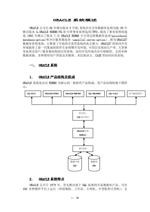
一、 ORACLE系统1．ORACLE产品结构及组成ORACLE系统是由以RDBMS为核心的一批软件产品构成，其产品结构轮廓下图所示：2．ORACLE系统特点ORACLE公司于1979年，首先推出基于SQL标准的关系数据库产品，可在100多种硬件平台上运行（所括微机、工作站、小型机、中型机和大型机），支持很多种操作系统。

用户的ORACLE应用可方便地从一种计算机配置移至另一种计算机配置上。

ORACLE的分布式结构可将数据和应用驻留在多台计算机上，而相互间的通信是透明的。

1992年6月ORACLE公司推出的ORACLE7协同服务器数据库，使关系数据库技术迈上了新台阶。

根据IDG（国际数据集团）1992年全球UNIX数据库市场报告，ORACLE占市场销售量50%。

它之所以倍受用户喜爱是因为它有以下突出的特点：●支持大数据库、多用户的高性能的事务处理。

ORACLE支持最大数据库，其大小可到几百千兆，可充分利用硬件设备。

支持大量用户同时在同一数据上执行各种数据应用，并使数据争用最小，保证数据一致性。

系统维护具有高的性能，ORACLE每天可连续24小时工作，正常的系统操作（后备或个别计算机系统故障）不会中断数据库的使用。

关于Oracle E-Business Suite并发处理机制（Current Processing）2015-01-21 14:05 2352人阅读评论(0) 收藏举报分类：Oracle EBS（48）Oracle EBS Concurrent Program（15）版权声明：转载请以链接形式注明出处2012年写过一篇关于Oracle E-Business Suite并发管理器的文章，回头看之前总结的内容还是比较单薄，很多点没说到，最近在看这块的内容，索性再写一篇稍微完整的文章来。

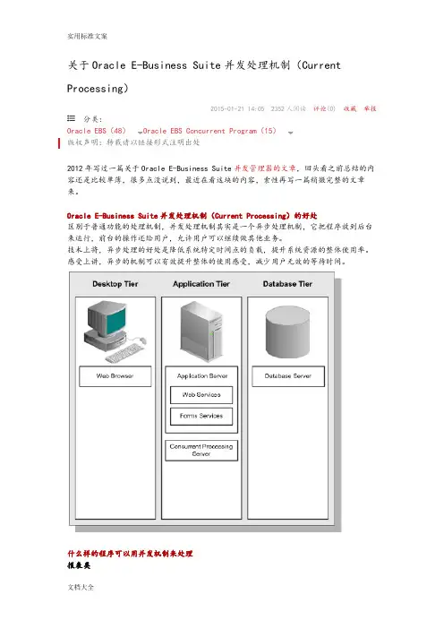
Oracle E-Business Suite并发处理机制（Current Processing）的好处区别于普通功能的处理机制，并发处理机制其实是一个异步处理机制，它把程序放到后台来运行，前台的操作还给用户，允许用户可以继续做其他业务。

技术上将，异步处理的好处是降低系统特定时间点的负载，提升系统资源的整体使用率。

感受上讲，异步的机制可以有效提升整体的使用感受，减少用户无效的等待时间。

什么样的程序可以用并发机制来处理报表类报表是一种非常个性化的东西，一般也是每家公司客户化最多的部分，如果为报表需求都开发不同的列表界面来查询、展示，那么工作量将是巨大的。

所以Oracle把报表嵌入到并发处理中，通过一些灵活的配置或少量的开发（Reports/BI Publisher Reports）既可以实现用户各类报表的需求.流程类多用于批量事务处理，或是长时间运行的业务，如库存管理器批量处理接口表中的临时事务。

并发处理机制（Current Processing）的两类组件并发处理机制（Current Processing）包括两类组件：•并发管理器（Concurrent Managers）•并发请求（Concurrent Requests）像公司中“经理”一样，Manager给Worker安排任务，Worker负责具体的执行。

Oracle EBS中的Concurrent Managers就是负责安排工作，Concurrent Requests负责具体的执行。

Oracle 优化和性能调整将要涉及的问题为了保证Oracle数据库运行在最佳的性能状态下，在信息系统开发之前就应该考虑数据库的优化策略。

优化策略一般包括服务器操作系统参数调整、数据库参数调整、网络性能调整、应用程序SQL语句分析及设计等几个方面，其中应用程序的分析与设计是在信息系统开发之前完成的。

分析评价Oracle数据库性能主要有数据库吞吐量、数据库用户响应时间两项指标。

数据库用户响应时间又可以分为系统服务时间和用户等待时间两项，即：数据库用户响应时间=系统服务时间＋用户等待时间因此，获得满意的用户响应时间有两个途径：一是减少系统服务时间，即提高数据库的吞吐量；二是减少用户等待时间，即减少用户访问同一数据库资源的冲突率。

数据库性能优化包括如下几个部分：∙调整数据结构的设计这一部分在开发信息系统之前完成，程序员需要考虑是否使用Oracle数据库的分区功能，对于经常访问的数据库表是否需要建立索引等。

∙调整应用程序结构设计这一部分也是在开发信息系统之前完成的。

程序员在这一步需要考虑应用程序使用什么样的体系结构，是使用传统的Client/Server两层体系结构，还是使用Browser/Web/Database的三层体系结构。

不同的应用程序体系结构要求的数据库资源是不同的。

∙调整数据库SQL语句应用程序的执行最终将归结为数据库中的SQL语句执行，因此SQL语句的执行效率最终决定了Oracle数据库的性能。

Oracle公司推荐使用Oracle语句优化器（Oracle Optimizer）和行锁管理器（Row-Level Manager）来调整优化SQL语句。

∙调整服务器内存分配内存分配是在信息系统运行过程中优化配置的。

数据库管理员根据数据库的运行状况不仅可以调整数据库系统全局区（SGA区）的数据缓冲区、日志缓冲区和共享池的大小，而且还可以调整程序全局区（PGA区）的大小。

∙调整硬盘I/O 这一步是在信息系统开发之前完成的。

DBA面试大全一：SQL tuning 类1:列举几种表连接方法答:merge join,hash join,nested loop2:不借助第三方对象，如何查看sql的履行筹划答:sqlplusset autotrace ...utlxplan.sql创建plan_table表3:若何应用CBO,CBO与RULE的差别答:在初始化参数里面设置optimizer_mode=choose/all_rows/first_row等能够应用cbo.<br />rbo会选择不合适的索引,cbo须要统计信息。

4:若何定位重要(消费资本多)的SQL答:依照v$sqlarea 中的逻辑读/disk_read。

以及查找CPU应用过量的session,查出当前session 的当前SQL语句，或者：监控WIN平台Oracle的运行5:若何跟踪某个session的SQL答:先找出对应的'sid,serial',然后调用system_system.set_sql_trace_in_session(sid,serial,true);参考：跟踪某个会话6:SQL调剂最存眷的是什么答:逻辑读。

IO量7:说说你对索引的熟悉（索引的构造、对dml阻碍、对查询阻碍、什么缘故进步查询机能答:默认的索引是b-tree.对insert的阻碍.(决裂，要包管tree的均衡)对delete的阻碍.(删除行的时刻要标记改节点为删除).对update的阻碍，假如更新表中的索引字段，则要响应的更新索引中的键值。

查询中包含索引字段的键值和行的物理地址。

8:应用索引查询必定能进步查询的机能吗？什么缘故答:不克不及。

假如返回的行数量较大年夜，应用全表扫描的机能较好。

9:绑定变量是什么？绑定变量有什么优缺点答:通俗的说，绑定变量确实是变量的一个占位符，应用绑定变量能够削减只有变量值不合的语句的解析。

10:若何稳固(固定)履行筹划答:应用stored outline.11:和排序相干的内存在8i和9i分别如何调剂，临时表空间的感化是什么答i：应用sort_area_size，hash_area_size,每个session分派雷同的值，不管有无应用。

Oracle 常见的33个等待事件等待事件的源起等待事件的概念大概是从ORACLE 7.0.12中引入的，大致有100个等待事件。

在ORACLE 8.0中这个数目增大到了大约150个，在ORACLE 8I中大约有220个事件，在ORACLE 9IR2中大约有400个等待事件，而在最近ORACLE 10GR2中，大约有874个等待事件。

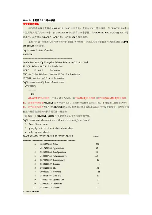
虽然不同版本和组件安装可能会有不同数目的等待事件，但是这些等待事件都可以通过查询V$EVE NT_NAME视图获得：SQL> select * from v$version;BANNER----------------------------------------------------------------Oracle Database 10g Enterprise Edition Release 10.2.0.1.0 - ProdPL/SQL Release 10.2.0.1.0 - ProductionCORE 10.2.0.1.0 ProductionTNS for 32-bit Windows: Version 10.2.0.1.0 - ProductionNLSRTL Version 10.2.0.1.0 –ProductionSQL> select count(*) from v$event_name;COUNT(*)----------872ORACLE的等待事件，主要可以分为两类，即空闲(IDLE)等待事件和非空闲(NON-IDLE)等待事件。

1). 空闲等待事件指ORACLE正等待某种工作，在诊断和优化数据库的时候，不用过多注意这部分事件。

2). 非空闲等待事件专门针对ORACLE的活动，指数据库任务或应用运行过程中发生的等待，这些等待事件是在调整数据库的时候需要关注与研究的。

下面来看一下ORACLE 10GR2中主要分类及各类等待事件的个数：SQL> select wait_class#,wait_class_id,wait_class,count(*) as "count"2 from v$event_name3 group by wait_class#,wait_class_id,wait_class4 order by wait_class#;WAIT_CLASS# WAIT_CLASS_ID WAIT_CLASS count----------- ------------- ------------------------------ ----------0 1893977003 Other 5881 4217450380 Application 122 3290255840 Configuration 233 4166625743 Administrative 464 3875070507 Concurrency 245 3386400367 Commit 16 2723168908 Idle 627 2000153315 Network 268 1740759767 User I/O 179 4108307767 System I/O 2410 2396326234 Scheduler 211 3871361733 Cluster 4712 rows selected.常见的空闲事件有:• dispatcher timer• lock element cleanup• Null event• parallel query dequeue wait• parallel query idle wait - Slaves• pipe get• PL/SQL lock timer• pmon timer- pmon• rdbms ipc messa ge• slave wait• smon timer• SQL*Net break/reset to client• SQL*Net message from client• SQL*Net message to client• SQL*Net more data to client• virtual circuit status• client message一些常见的非空闲等待事件有:• db file scattered read• db file sequential read• buffer busy waits• free buffer waits• enqueue• latch free• log file parallel write• log file sync几个视图的总结：V$SESSION 代表数据库活动的开始，视为源起。