MathRep2
- 格式:doc
- 大小:583.50 KB
- 文档页数:24
mathematica 二次曲面标准型二次曲面是三维空间中的曲面,它的数学表达式可以写成一个二次方程。
二次曲面的标准型就是这个二次方程化简之后的形式,可以用来描述和研究二次曲面的性质和特点。
本文将主要介绍二次曲面的标准型,并对其中的一些常见类型进行详细说明。
二次曲面的标准型一般可以写成以下形式的方程:Ax^2 + By^2 + Cz^2 + Dxy + Exz + Fyz + Gx + Hy + Iz + J = 0其中A、B、C、D、E、F、G、H、I、J都是实数,且A、B、C均不为零。
这个方程描述了一个二次曲面在三维空间中的形状。
下面将对其中的每一项进行解释和说明。
首先,前三项Ax^2 + By^2 + Cz^2是描述二次曲面的平方项,它们决定了二次曲面是一个椭圆、双曲线还是一个抛物面。
当A、B、C都为正数时,二次曲面是一个椭球面,它在三个坐标轴方向上分别有一个焦点,可以看作是一个立体的椭圆。
当A、B、C中有一个为零,而另外两个都不为零时,二次曲面是一个抛物面。
若A或B为零,那么二次曲面将在竖直方向上呈现开口向上或向下的抛物线形状;若A、B都不为零,而C为零,则二次曲面在斜线方向上呈现开口向上或向下的抛物线形状。
当A、B、C中有一个为正,而另外两个为负时,二次曲面是一个单叶双曲面。
这种曲面在两个焦点之间呈现开口向上或向下的双曲线形状。
当A、B、C中有两个都为负时,二次曲面是一个双叶双曲面。
这种曲面在两个焦点之间呈现开口向外的双曲线形状。
第四至第六项Dxy + Exz + Fyz描述了二次曲面平面交线的倾斜程度。
它们决定了二次曲面在平面交线上的形状,包括圆锥曲线、椭圆锥面、双曲锥面和抛物锥面等。
根据这些项的系数可以确定二次曲面的倾斜程度和角度。
最后,第七至第十项Gx + Hy + Iz + J是描述平面和坐标轴的直线方程。
这些项决定了二次曲面平面的位置和方向。
通过计算这些项的系数,可以得到二次曲面相对于坐标轴的位置、倾斜角度和交点等信息。

math.random()方法是用来表示一、概述Math.random()是JavaScript中的一个方法,它被用于生成一个伪随机数。
这个方法可以返回一个介于0(包含)至指定精度的最大整数(不包含)之间的随机数。
精度的默认值是1/2^32,这意味着它可以产生大约1亿个唯一的数字。
这个方法对于生成随机的数值或决定游戏中的事件非常有用。
二、用法Math.random()方法返回一个介于0(包括)和1(不包括)之间的伪随机数。
如果需要更大的范围,可以调用Math.random()两次,例如Math.random()*100。
这将返回一个介于0至99之间的随机整数。
三、特点Math.random()方法的特点在于它的随机性。
生成的数字是基于一个复杂的算法产生的,该算法使用熵源(通常包括当前的时间、系统负载和处理器时钟速度)来产生随机数。
这种随机性使得Math.random()生成的数字在很多情况下具有实际的应用价值。
四、应用场景Math.random()方法在许多场景中都有应用,以下是几个常见的应用:1. 游戏随机事件:在游戏中,常常需要随机事件来增加游戏的趣味性和挑战性。
例如,一个角色可能会遇到一个随机的敌人,或者一个宝箱可能会被打开并获得一个随机的奖励。
使用Math.random()方法可以很容易地实现这些效果。
2. 数值生成:在需要随机数值的场景中,Math.random()方法也很有用。
例如,在模拟系统中,需要生成一系列随机的数据来代表各种情况。
使用Math.random()方法可以方便地生成这些数据。
3. 密码生成:在一些需要生成密码的场景中,Math.random()方法也可以派上用场。
通过将随机数与用户名或其他信息结合,可以生成一个独特的密码,增加了密码的安全性。
五、注意事项虽然Math.random()方法生成的数字看起来是随机的,但实际上它们是有规律的。
这是因为它们是基于算法生成的,而不是真正的随机数。
math.evaluate用法全文共四篇示例,供读者参考第一篇示例:math.evaluate是一个用于执行数学表达式的JavaScript函数。
它可以帮助用户计算和解析包含数学表达式的字符串,并返回结果。
在处理动态生成的数学表达式时,math.evaluate可以提供很大的便利性。
在日常开发中,我们经常需要对一些数学表达式进行计算,比如计算一个动态生成的数学公式的结果。
这时,使用math.evaluate就可以方便地完成这一任务。
下面我们来看一下如何使用math.evaluate来进行计算。
我们需要引入math.js库。
math.js是一个强大的数学库,它提供了丰富的数学函数和工具,可以方便地进行数学运算和计算。
可以通过在项目中引入math.js库,来使用其中的math.evaluate函数。
在开始使用math.evaluate之前,我们需要确保已经引入了math.js库。
接下来,我们可以使用如下的代码示例来计算一个简单的数学表达式:```javascriptconst math = require('math.js');// 定义一个包含数学表达式的字符串const expression = "2 + 3 * 4";// 输出计算结果console.log(result); // 输出14```在上面的示例中,我们首先引入了math.js库,然后定义了一个包含数学表达式的字符串"2 + 3 * 4"。
接着使用math.evaluate函数对该表达式进行计算,最后输出计算结果14。
除了简单的加减乘除运算外,math.evaluate还支持更复杂的数学运算,比如三角函数、指数函数、对数函数等。
我们可以通过传入包含这些函数的数学表达式来计算它们的结果。
下面是一个包含三角函数的数学表达式的示例:// 定义变量的值const x = 3;// 使用math.evaluate计算数学表达式的结果const result = math.evaluate(expression, { x });第二篇示例:math.evaluate()是JavaScript中一个非常有用的函数,它可以将一个字符串作为数学表达式来计算。
mathpow函数用法math.pow()是Javascript中数学方法的一种,它的功能是用来计算某个数的幂。
1. 什么是math.pow()?math.pow()是JavaScript中一种数学方法,可以用来计算某个数的幂。
它的格式是Math.pow(底数, 指数),返回的是一个 Number 类型的值。
2. math.pow()函数的参数math.pow()函数有两个参数:底数和指数。
底数是被提升的数字,指数是提升次数,幂的结果就是将底数依据指数提升的结果。
3. math.pow()函数的作用math.pow()的作用就是计算一个数的幂,让我们更容易地把一个数字提升成某个指定的次数。
比如,一个数字3,提升3次方,就是用math.pow(3, 3),就可以高效地得到结果 27,而不需要用乘法去一步步地把 3 乘以 3 再乘以 3。
4. math.pow()函数的用法math.pow函数的用法很简单,只需要两个参数,即底数和指数,就可以轻松计算出某个数的幂。
格式是Math.pow(底数, 指数),计算结束之后会返回一个 Number 类型的值。
比如让我们计算9的4次方,就可以用Math.pow(9,4),就可以得到结果6561,而不用写出9x9x9x9的乘法。
5. 一些示例(1)Math.pow(2,3) 结果为8,即2的3次方。
(2)Math.pow(3,2) 结果为9,即3的2次方。
(3)Math.pow(4,4) 结果为256,即4的4次方。
6. 总结math.pow()是JavaScript中一种很有用的数学方法,它可以让我们高效、精确地计算某个数的幂,省去人肉一步一步用乘法计算繁琐的过程,两个参数让我们可以快速得到想要的结果。
math.random 函数用法math.random函数是Lua中用于生成随机数的函数。
它可以接受一个或两个参数。
如果只传递一个参数n,则函数会返回一个[1, n]之间的整数随机数。
例如,math.random(10)会返回一个1~10之间的整数。
如果传递两个参数min和max,则函数会返回一个[min, max]之间的整数随机数。
例如,math.random(1, 10)会返回一个1~10之间的整数。
需要注意的是,math.random函数在每次调用时会返回一个完全随机的值,即使传递的参数相同也会返回不同的随机数。
如果需要生成伪随机数序列,应该使用math.randomseed函数来初始化随机数种子。
下面举例详细说明。
当我们使用math.random函数时,它会生成一个随机数。
为了方便演示,我们假设我们正在开发一个随机点名的程序,需要在已有姓名列表中随机选择一个人进行点名。
首先,我们需要定义一个含有所有姓名的列表:```names = {"Tom", "Jack", "Sarah", "Amy", "John", "Kate"}```然后,我们可以使用math.random函数来选择一个随机的姓名。
我们可以使用列表的长度作为上限,最终得到一个[1, length]之间的整数,这个整数对应着一个姓名:```--生成一个随机的姓名randomIndex = math.random(#names)selectedName = names[randomIndex]--输出随机的姓名print("The selected name is: " .. selectedName)```这段代码会输出一个随机的姓名,例如:"The selected name is: Kate"。
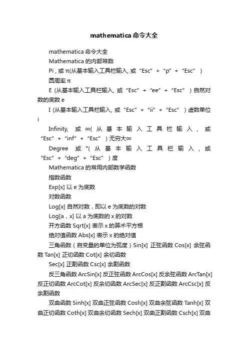
mathematica命令大全mathematica命令大全Mathematica的内部常数Pi , 或π(从基本输入工具栏输入, 或“Esc”+“p”+“Esc”)圆周率πE (从基本输入工具栏输入, 或“Esc”+“ee”+“Esc”)自然对数的底数eI (从基本输入工具栏输入, 或“Esc”+“ii”+“Esc”)虚数单位iInfinity, 或∞(从基本输入工具栏输入, 或“Esc”+“inf”+“Esc”)无穷大∞Degree 或°(从基本输入工具栏输入,或“Esc”+“deg”+“Esc”)度Mathematica的常用内部数学函数指数函数Exp[x] 以e为底数对数函数Log[x] 自然对数,即以e为底数的对数Log[a,x] 以a为底数的x的对数开方函数Sqrt[x] 表示x的算术平方根绝对值函数Abs[x] 表示x的绝对值三角函数(自变量的单位为弧度)Sin[x] 正弦函数Cos[x] 余弦函数Tan[x] 正切函数Cot[x] 余切函数Sec[x] 正割函数Csc[x] 余割函数反三角函数ArcSin[x] 反正弦函数ArcCos[x] 反余弦函数ArcT an[x] 反正切函数ArcCot[x] 反余切函数ArcSec[x] 反正割函数ArcCsc[x] 反余割函数双曲函数Sinh[x] 双曲正弦函数Cosh[x] 双曲余弦函数Tanh[x] 双曲正切函数Coth[x] 双曲余切函数Sech[x] 双曲正割函数Csch[x] 双曲余割函数反双曲函数ArcSinh[x] 反双曲正弦函数ArcCosh[x] 反双曲余弦函数ArcTanh[x] 反双曲正切函数ArcCoth[x] 反双曲余切函数ArcSech[x] 反双曲正割函数ArcCsch[x] 反双曲余割函数求角度函数ArcTan[x,y]以坐标原点为顶点,x轴正半轴为始边,从原点到点(x,y)的射线为终边的角,其单位为弧度数论函数GCD[a,b,c,...] 最大公约数函数LCM[a,b,c,...] 最小公倍数函数Mod[m,n] 求余函数(表示m 除以n的余数)Quotient[m,n] 求商函数(表示m除以n的商)Divisors[n] 求所有可以整除n的整数FactorInteger[n] 因数分解,即把整数分解成质数的乘积Prime[n] 求第n个质数PrimeQ[n]判断整数n是否为质数,若是,则结果为True,否则结果为FalseRandom[Integer,{m,n}] 随机产生m到n之间的整数排列组合函数Factorial[n]或n!阶乘函数,表示n的阶乘复数函数Re[z] 实部函数Im[z] 虚部函数Arg(z) 辐角函数Abs[z] 求复数的模Conjugate[z] 求复数的共轭复数Exp[z] 复数指数函数求整函数与截尾函数Ceiling[x] 表示大于或等于实数x的最小整数Floor[x] 表示小于或等于实数x的最大整数Round[x] 表示最接近x的整数IntegerPart[x] 表示实数x的整数部分FractionalPart[x] 表示实数x的小数部分分数与浮点数运算函数N[num]或num//N 把精确数num化成浮点数(默认16位有效数字)N[num,n] 把精确数num化成具有n个有效数字的浮点数NumberForm[num,n] 以n个有效数字表示num Rationalize[float] 将浮点数float转换成与其相等的分数Rationalize[float,dx] 将浮点数float转换成与其近似相等的分数,误差小于dx最大、最小函数Max[a,b,c,...] 求最大数Min[a,b,c,...] 求最小数符号函数Sign[x]Mathematica中的数学运算符a+b加法a-b 减法a*b (可用空格键代替*) 乘法a/b (输入方法为:“ Ctrl ” + “ / ” )除法a^b (输入方法为:“ Ctrl ” + “ ^” )乘方-a 负号Mathematica的关系运算符==等于< 小于> 大于<= 小于或等于>= 大于或等于!= 不等于注:上面的关系运算符也可从基本输入工具栏输入。
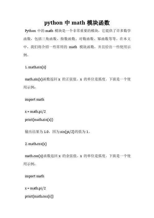
python中math模块函数Python中的math模块是一个非常重要的模块,它提供了许多数学函数,包括三角函数、指数函数、对数函数、幂函数等等。
在本文中,我们将介绍一些常用的math模块函数,并且给出一些使用示例。
1. math.sin(x)math.sin(x)函数返回x的正弦值。
x的单位是弧度。
下面是一个使用示例:import mathx = math.pi/2print(math.sin(x))输出结果为1.0,因为sin(pi/2)的值为1。
2. math.cos(x)math.cos(x)函数返回x的余弦值。
x的单位是弧度。
下面是一个使用示例:import mathx = math.pi/2print(math.cos(x))输出结果为6.123233995736766e-17,因为cos(pi/2)的值为0。
3. math.tan(x)math.tan(x)函数返回x的正切值。
x的单位是弧度。
下面是一个使用示例:import mathx = math.pi/4print(math.tan(x))输出结果为1.0,因为tan(pi/4)的值为1。
4. math.exp(x)math.exp(x)函数返回e的x次幂。
下面是一个使用示例:import mathx = 2print(math.exp(x))输出结果为7.3890560989306495,因为e的2次幂的值为7.3890560989306495。
5. math.log(x)math.log(x)函数返回x的自然对数。
下面是一个使用示例:import mathx = 10print(math.log(x))输出结果为2.302585092994046,因为e的2.302585092994046次幂的值为10。
6. math.pow(x, y)math.pow(x, y)函数返回x的y次幂。
下面是一个使用示例:import mathx = 2y = 3print(math.pow(x, y))输出结果为8.0,因为2的3次幂的值为8。
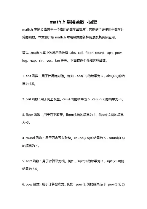
math.h常用函数-回复math.h库是C语言中一个常用的数学函数库,它提供了许多用于数学计算的函数。
本文将介绍math.h常用函数的各种用法及其实际应用。
首先,math.h库中的常用函数有:abs、ceil、floor、round、sqrt、pow、log、exp、sin、cos、tan等等。
下面将逐个介绍这些函数。
1. abs函数:用于计算绝对值。
例如,abs(-5)的结果为5,abs(4.5)的结果为4.5。
2. ceil函数:用于向上取整。
ceil(4.2)的结果为5,ceil(-3.7)的结果为-3。
3. floor函数:用于向下取整。
floor(4.9)的结果为4,floor(-2.3)的结果为-3。
4. round函数:用于四舍五入取整。
round(4.5)的结果为5,round(4.4)的结果为4。
5. sqrt函数:用于计算平方根。
例如,sqrt(9)的结果为3,sqrt(25.0)的结果为5.0。
6. pow函数:用于计算幂次方。
例如,pow(2, 3)的结果为8,pow(3.5, 2)的结果为12.25。
7. log函数:用于计算自然对数。
例如,log(1.0)的结果为0,log(10.0)的结果为2.3026。
8. exp函数:用于计算指数函数。
例如,exp(1.0)的结果为2.7183,exp(2.5)的结果为12.1825。
9. sin函数:用于计算正弦值。
例如,sin(0)的结果为0,sin(3.14/2)的结果为1。
10. cos函数:用于计算余弦值。
例如,cos(0)的结果为1,cos(3.14)的结果为-1。
11. tan函数:用于计算正切值。
例如,tan(0)的结果为0,tan(3.14/4)的结果为1。
下面将就每个函数的实际应用进行更详细的介绍。
1. abs函数广泛应用于计算绝对值,常用于计算两个数的差值时取绝对值以保证结果的准确性。
2. ceil和floor函数可以用于数学运算的精确性控制。
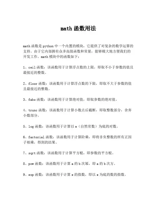
math函数用法math函数是python中一个内置的模块,它提供了对复杂的数学运算的支持。
由于它内部拥有众多高级函数和常量,能够极大地方便我们的开发工作。
math模块中的函数如下:1、ceil函数:该函数用于计算浮点数的上限,即取不小于参数的值且最接近的整数。
2、floor函数:该函数用于计算浮点数的下限,即取不大于参数的值且最接近的整数。
3、fabs函数:该函数用于计算绝对值,即取参数的绝对值。
4、trunc函数:该函数用于计算小数点后截断,即取整数部分,舍弃小数部分。
5、log函数:该函数用于计算以e(自然常数)为底的对数。
6、factorial函数:该函数用于计算阶乘,即将非负整数的所有正因子相乘,得到的结果。
7、sqrt函数:该函数用于计算平方根,即参数的平方根。
8、pow函数:该函数用于计算a的b次幂,即a的b次方。
9、exp函数:该函数用于计算e的指数,即以e为底的数的指数。
10、cos函数:该函数用于计算余弦,即求出x的余弦值。
11、sin函数:该函数用于计算正弦,即求出x的正弦值。
12、tan函数:该函数用于计算正切,即求出x的正切值。
13、atan函数:该函数用于计算反正切,即求出tanx-1的值。
使用math模块时,需要先import math,然后在使用的时候通过math.函数名来调用,例如计算fabs(3.4),可以写成:import mathfabs_res = math.fabs(3.4)print(fabs_res)运行结果为:3.4从上述内容可以看出,math模块提供了众多实用的函数,能够帮助开发者更加有效地完成相应的数学运算。
在具体开发中,我们始终要注意使用必要的函数,并保持函数的调用参数合理,这样才能有效地保证代码的可操作性。

分区中文分类刊名简称1 地学ACTA ASTRONOM1 地学ADV GEOPHYS1 地学AM J SCI1 地学 B AM METEOROL SOC1 地学CLIM DYNAM1 地学J CLIMATE1 地学J PETROL1 地学LIMNOL OCEANOGR1 地学QUATERNARY SCI REV1 地学REV GEOPHYS1 地学TELLUS B2 地学AM MINERAL2 地学CHEM GEOL2 地学EARTH PLANET SC LETT2 地学GEOCHIM COSMOCHIM AC2 地学GEOLOGY2 地学GEOPHYS RES LETT2 地学J GEOPHYS RES2 地学J ATMOS SCI2 地学MON WEATHER REV1 地学天文ANNU REV ASTRON ASTR 1 地学天文ASTROPHYS J1 工程技术ACTA MATER1 工程技术ADV MATER1 工程技术AICHE J1 工程技术ANNU REV BIOMED ENG1 工程技术APPL SPECTROSC1 工程技术ARTIF INTELL1 工程技术ARTIF LIFE1 工程技术BIOMATERIALS1 工程技术CHEM VAPOR DEPOS1 工程技术CHEM MATER1 工程技术COGNITIVE BRAIN RES 1 工程技术COMMUN ACM1 工程技术CRIT REV FOOD SCI1 工程技术DIAM RELAT MATER1 工程技术ESA BULL-EUR SPACE1 工程技术EUR PHYS J E1 工程技术HUM-COMPUT INTERACT 1 工程技术IBM J RES DEV1 工程技术IEEE COMMUN MAG1 工程技术IEEE CONTR SYST MAG 1 工程技术IEEE ELECTR DEVICE L 1 工程技术IEEE J QUANTUM ELECT 1 工程技术IEEE J SEL TOP QUANT 1 工程技术IEEE J SEL AREA COMM 1 工程技术IEEE NETWORK1 工程技术IEEE PERS COMMUN1 工程技术IEEE PHOTONIC TECH L 1 工程技术IEEE SIGNAL PROC MAG 1 工程技术IEEE T ELECTRON DEV 1 工程技术IEEE T IMAGE PROCESS1 工程技术IEEE T VIS COMPUT GR 1 工程技术IEEE ACM T NETWORK1 工程技术INFORM SYST1 工程技术INT J COMPUT VISION 1 工程技术INT J FOOD MICROBIOL 1 工程技术J FOOD PROTECT1 工程技术J LIGHTWAVE TECHNOL 1 工程技术J MACH LEARN RES1 工程技术J MATER CHEM1 工程技术J MEMBRANE SCI1 工程技术J MICROELECTROMECH S 1 工程技术J NANOSCI NANOTECHNO 1 工程技术J SUPERCRIT FLUID1 工程技术J AM CERAM SOC1 工程技术J AM SOC INF SCI TEC 1 工程技术MAT SCI ENG R1 工程技术MED IMAGE ANAL1 工程技术MIS QUART1 工程技术MRS BULL1 工程技术MRS INTERNET J N S R 1 工程技术NANO LETT1 工程技术NEURAL COMPUT1 工程技术P IEEE1 工程技术PROG ENERG COMBUST1 工程技术PROG MATER SCI1 工程技术PROG QUANT ELECTRON1 工程技术ULTRAMICROSCOPY2 工程技术APPL SURF SCI2 工程技术AUTOMATICA2 工程技术CEREAL CHEM2 工程技术CHEM ENG SCI2 工程技术CORROS SCI2 工程技术ELECTRON LETT2 工程技术FOOD CHEM2 工程技术IEEE J SOLID-ST CIRC 2 工程技术IEEE T ANTENN PROPAG 2 工程技术IEEE T APPL SUPERCON 2 工程技术IEEE T AUTOMAT CONTR 2 工程技术IEEE T BIO-MED ENG2 工程技术IEEE T COMMUN2 工程技术IEEE T COMPUT2 工程技术IEEE T INFORM THEORY 2 工程技术IEEE T MICROW THEORY 2 工程技术IEEE T NUCL SCI2 工程技术IEEE T SIGNAL PROCES 2 工程技术IND ENG CHEM RES2 工程技术INT J NUMER METH ENG 2 工程技术J AGR FOOD CHEM2 工程技术J ELECTRON MATER2 工程技术J FOOD SCI2 工程技术J MATER RES2 工程技术J NON-CRYST SOLIDS2 工程技术J NUCL MATER2 工程技术J POWER SOURCES2 工程技术J AM OIL CHEM SOC2 工程技术J EUR CERAM SOC2 工程技术J VAC SCI TECHNOL A 2 工程技术MAT SCI ENG A-STRUCT 2 工程技术METALL MATER TRANS A 2 工程技术REV SCI INSTRUM2 工程技术SCRIPTA MATER2 工程技术SENSOR ACTUAT A-PHYS 2 工程技术SENSOR ACTUAT B-CHEM 2 工程技术SURF COAT TECH2 工程技术SYNTHETIC MET2 工程技术THIN SOLID FILMS1 管理科学ADV STUD BEHAV1 管理科学J MATH PSYCHOL1 管理科学J OPER MANAG1 管理科学J EXP ANAL BEHAV2 管理科学MANAGE SCI2 管理科学OPER RES2 管理科学TECHNOMETRICS1 化学ACCOUNTS CHEM RES1 化学ADV CATAL1 化学ADV INORG CHEM1 化学ADV ORGANOMET CHEM1 化学ADV PHYS ORG CHEM1 化学ADV POLYM SCI1 化学ALDRICHIM ACTA1 化学ANGEW CHEM INT EDIT1 化学ANNU REV PHYS CHEM1 化学CATAL REV1 化学CHEM REV1 化学CHEM SOC REV1 化学J PHYS CHEM REF DATA 1 化学J AM CHEM SOC1 化学PROG INORG CHEM1 化学SURF SCI REP1 化学TOP CURR CHEM2 化学ANAL CHEM2 化学CHEM COMMUN2 化学ELECTROPHORESIS2 化学INORG CHEM2 化学J CHROMATOGR A2 化学J ORG CHEM2 化学J PHYS CHEM B2 化学LANGMUIR2 化学MACROMOLECULES2 化学ORG LETT2 化学ORGANOMETALLICS1 环境科学ADV ECOL RES1 环境科学AM NAT1 环境科学ANNU REV ECOL SYST 1 环境科学CONSERV ECOL1 环境科学ECOL APPL1 环境科学ECOL MONOGR1 环境科学ECOLOGY1 环境科学GLOBAL BIOGEOCHEM CY1 环境科学GLOBAL CHANGE BIOL2 环境科学ATMOS ENVIRON2 环境科学ENVIRON HEALTH PERSP 2 环境科学ENVIRON SCI TECHNOL 2 环境科学ENVIRON TOXICOL CHEM 2 环境科学MAR ECOL-PROG SER2 环境科学MOL ECOL2 环境科学OECOLOGIA2 环境科学OIKOS1 农林科学ADV AGRON1 农林科学AGR FOREST METEOROL 1 农林科学CAN J FISH AQUAT SCI 1 农林科学DIS AQUAT ORGAN1 农林科学DOMEST ANIM ENDOCRIN 1 农林科学J ANIM SCI1 农林科学J DAIRY SCI1 农林科学REV FISH BIOL FISHER 1 农林科学SOIL BIOL BIOCHEM1 农林科学TREE PHYSIOL2 农林科学AQUACULTURE2 农林科学CAN J FOREST RES2 农林科学FOREST ECOL MANAG2 农林科学J SCI FOOD AGR2 农林科学PLANT SOIL2 农林科学POULTRY SCI2 农林科学SOIL SCI SOC AM J1 社会科学ECONOMETRICA2 社会科学MED EDUC1 生物AM J HUM GENET1 生物ANNU REV BIOCHEM1 生物ANNU REV BIOPH BIOM1 生物ANNU REV CELL DEV BI 1 生物ANNU REV GENET1 生物ANNU REV MICROBIOL1 生物ANNU REV PHYSIOL1 生物ANNU REV PLANT PHYS1 生物BBA-REV BIOMEMBRANES 1 生物BIOESSAYS1 生物CELL1 生物CURR BIOL1 生物CURR OPIN CELL BIOL1 生物CURR OPIN GENET DEV1 生物CURR OPIN PLANT BIOL 1 生物CURR OPIN STRUC BIOL 1 生物CYTOKINE GROWTH F R1 生物DEVELOPMENT1 生物DEV CELL1 生物EMBO J1 生物FASEB J1 生物FEMS MICROBIOL REV1 生物GENE DEV1 生物HUM MOL GENET1 生物J CELL BIOL1 生物MICROBIOL MOL BIOL R 1 生物MOL CELL BIOL1 生物MOL BIOL CELL1 生物MOL CELL1 生物NAT BIOTECHNOL1 生物NAT CELL BIOL1 生物NAT GENET1 生物NAT REV GENET1 生物NAT REV MOL CELL BIO 1 生物NAT STRUCT BIOL1 生物PLANT CELL1 生物PROG NUCLEIC ACID RE 1 生物TRENDS BIOCHEM SCI 1 生物TRENDS CELL BIOL1 生物TRENDS ECOL EVOL1 生物TRENDS GENET1 生物TRENDS PLANT SCI2 生物AM J PHYSIOL-CELL PH 2 生物APPL ENVIRON MICROB 2 生物BIOCHEM J2 生物BIOCHEMISTRY-US2 生物BIOL REPROD2 生物BIOPHYS J2 生物DEV BIOL2 生物FEBS LETT2 生物GENETICS2 生物J BACTERIOL2 生物J BIOL CHEM2 生物J CELL SCI2 生物J CLIN MICROBIOL2 生物J MOL BIOL2 生物MOL MICROBIOL2 生物NUCLEIC ACIDS RES2 生物PLANT J2 生物PLANT PHYSIOL1 数学ACTA MATH-DJURSHOLM 1 数学ANN MATH1 数学APPL COMPUT HARMON A 1 数学 B AM MATH SOC1 数学COMMUN PUR APPL MATH 1 数学INVENT MATH1 数学J AM MATH SOC1 数学J AM STAT ASSOC1 数学J ROY STAT SOC A STA 1 数学J ROY STAT SOC B1 数学MEM AM MATH SOC1 数学SIAM J NUMER ANAL1 数学SIAM J OPTIMIZ1 数学SIAM REV1 数学STAT SCI2 数学ANN STAT2 数学INT J BIFURCAT CHAOS 2 数学J DIFFER EQUATIONS 2 数学MATH COMPUT2 数学SIAM J CONTROL OPTIM 2 数学SIAM J SCI COMPUT1 物理ADV NUCL PHYS1 物理ADV PHYS1 物理ANNU REV FLUID MECH 1 物理ANNU REV NUCL PART S 1 物理EUR PHYS J C1 物理J HIGH ENERGY PHYS 1 物理MASS SPECTROM REV1 物理NUCL PHYS B1 物理PHYS REV LETT1 物理PHYS REP1 物理PHYS TODAY1 物理PROG NUCL MAG RES SP 1 物理PROG OPTICS1 物理REP PROG PHYS1 物理REV MOD PHYS1 物理SOLID STATE PHYS2 物理APPL PHYS LETT2 物理CHEM PHYS LETT2 物理J APPL PHYS2 物理J CHEM PHYS2 物理OPT LETT2 物理PHYS REV A2 物理PHYS REV B2 物理PHYS REV C2 物理PHYS REV D2 物理PHYS REV E2 物理PHYS LETT B1 医学ADV CANCER RES1 医学ADV IMMUNOL1 医学AIDS1 医学AM J MED1 医学AM J PATHOL1 医学AM J PSYCHIAT1 医学AM J RESP CRIT CARE 1 医学ANN INTERN MED1 医学ANN NEUROL1 医学ANN SURG1 医学ANNU REV GENOM HUM G 1 医学ANNU REV IMMUNOL1 医学ANNU REV MED1 医学ANNU REV NEUROSCI1 医学ANNU REV NUTR1 医学ANNU REV PHARMACOL 1 医学ANNU REV PSYCHOL1 医学ANTIVIR THER1 医学ARCH GEN PSYCHIAT1 医学ARCH INTERN MED1 医学ARTERIOSCL THROM VAS1 医学ARTHRITIS RHEUM1 医学ATHEROSCLEROSIS SUPP1 医学BEHAV BRAIN SCI1 医学BBA-REV CANCER1 医学BLOOD1 医学BRAIN1 医学BRAIN PATHOL1 医学BRAIN RES REV1 医学BRIT MED J1 医学CA-CANCER J CLIN1 医学CANCER RES1 综合性期刊NATURE1 综合性期刊P NATL ACAD SCI USA 1 综合性期刊SCIENCE。
math.evaluate用法全文共四篇示例,供读者参考第一篇示例:math.evaluate是一个用于解析和计算数学表达式的JavaScript 库。
它可以将字符串表示的数学表达式转换为可执行的JavaScript代码,并返回结果。
这个库的主要优点是它可以通过传递字符串参数来动态计算表达式,而不需要预先编写和存储计算逻辑。
下面将介绍一些关于math.evaluate用法的重要内容。
1. 如何安装math.evaluate要使用math.evaluate,首先需要安装math.js库。
可以通过npm或者直接在浏览器中引入math.js文件来安装。
安装完成后,就可以通过以下方式引入math.evaluate函数:```javascriptconst math = require('math.js');```expression是要计算的数学表达式的字符串表示,scope是一个可选的对象,用于定义要在表达式中使用的变量。
我们要计算2+3的结果:3. 支持的数学运算符和函数math.evaluate支持大多数基本的数学运算符和函数,包括加减乘除、乘方、开方、三角函数等。
可以计算sin(π/2)的结果:4. 使用变量如果需要在表达式中使用变量,可以在scope对象中定义变量,并将其作为第二个参数传递给math.evaluate函数。
计算一个变量的平方根:5. 复杂表达式的计算math.evaluate还支持复杂的数学表达式,例如嵌套的运算和函数调用。
可以使用括号来定义运算的优先级。
计算一个多项式的值:```javascriptmath.evaluate('(3*x^2 + 5*x + 2)', { x: 2 });// 输出:18```6. 错误处理如果表达式不符合数学规则,或者无法计算,math.evaluate将返回一个Error对象。
可以通过try-catch语句来捕获并处理错误。
math.random()方法用来表示数学领域中,Math.random()方法是一个非常常用的函数,它用于生成一个介于0(包括)和指定范围内的一个随机数。
这个方法可以用于各种应用场景,包括游戏、抽奖、模拟、数据分析等。
下面我们将详细讨论Math.random()方法的应用场景和实际使用方法。
一、生成随机数Math.random()方法最直接的应用场景就是生成随机数。
在数学上,0.0表示没有数,而1.0表示所有的数。
所以,我们可以通过这个方法生成一个在[0, 1)之间的随机浮点数。
如果需要更大的随机数范围,只需要在调用Math.random()时传入一个参数即可。
例如,Math.random(10)将返回一个介于[0, 9)之间的随机整数。
二、模拟抽奖在游戏中,我们经常需要模拟抽奖过程。
例如,一个游戏需要从多个玩家中随机选择一个作为幸运儿。
这种情况下,我们可以使用Math.random()方法来生成一个随机数,然后根据这个随机数来确定幸运儿。
这种方法简单易行,而且公平公正。
三、随机排列在数据分析和机器学习中,我们经常需要对数据进行随机排列以观察不同组合的效果。
例如,在实验设计中,我们可能需要观察不同的实验组合对结果的影响。
这种情况下,我们可以使用Math.random()方法来随机排列数据,从而得到不同的实验组合。
四、数据驱动决策在一些决策模型中,我们可以通过观察数据并使用Math.random()方法来生成随机建议或决策。
例如,在一个推荐系统中,我们可以通过分析用户的历史行为和偏好,使用Math.random()方法来生成一个随机建议,从而增加系统的多样性。
五、游戏开发中的随机元素在游戏开发中,Math.random()方法被广泛用于创造各种随机事件和元素。
例如,在一个冒险游戏中,玩家可能会遇到一个随机的怪物或宝藏;在一个策略游戏中,玩家可能会在地图上随机生成资源点或敌人基地。
这些随机元素可以为游戏增加趣味性和挑战性。
math库中的数学函数Math库是Python中内置的数学函数库,提供了一系列用于执行数学运算的函数和常量。
以下是Math库中的一些常用的数学函数:1.数值函数:- ceil(x): 返回大于或等于x的最小整数。
- floor(x): 返回小于或等于x的最大整数。
- round(x, n): 返回x的四舍五入值,n是可选的小数位数,如果省略则默认为0。
- trunc(x): 返回x的整数部分。
- fabs(x): 返回x的绝对值。
- sqrt(x): 返回x的平方根。
- pow(x, y): 返回x的y次方。
- exp(x): 返回e的x次方。
- log(x): 返回x的自然对数。
- log10(x): 返回x的以10为底的对数。
2.三角函数:- sin(x): 返回x的正弦值,x的单位是弧度。
- cos(x): 返回x的余弦值,x的单位是弧度。
- tan(x): 返回x的正切值,x的单位是弧度。
- asin(x): 返回x的反正弦值,返回值在 -pi/2 到 pi/2 之间。
- acos(x): 返回x的反余弦值,返回值在 0 到 pi 之间。
- atan(x): 返回x的反正切值,返回值在 -pi/2 到 pi/2 之间。
- atan2(y, x): 返回y / x的反正切值,返回值在 -pi 到 pi 之间。
3.超越函数:- sinh(x): 返回x的双曲正弦值。
- cosh(x): 返回x的双曲余弦值。
- tanh(x): 返回x的双曲正切值。
- asinh(x): 返回x的反双曲正弦值。
- acosh(x): 返回x的反双曲余弦值。
- atanh(x): 返回x的反双曲正切值。
4.统计函数:- sum(iterable): 返回可迭代对象中的所有元素之和。
- max(iterable): 返回可迭代对象中的最大值。
- min(iterable): 返回可迭代对象中的最小值。
- mean(iterable): 返回可迭代对象中所有元素的算术平均值。
math.random()方法生成的随机整数概述说明以及解释1. 引言1.1 概述在计算机编程中,随机数的生成对于许多应用程序来说是至关重要的。
而在JavaScript语言中,我们可以使用Math对象的random()方法来生成随机数。
本文将对这个方法进行全面的概述和解释。
1.2 目的本篇文章旨在介绍Math对象的random()方法以及通过该方法生成的随机整数。
我们将详细探讨该方法的使用注意事项、原理分析、优缺点分析,并与其他随机数生成方法进行比较。
通过深入了解这个方法,读者能够更好地理解它的特点和适用场景,并且能够在实际应用中做出明智的决策。
1.3 结构本文将按照以下结构展开对Math.random()方法生成随机整数的说明:第2部分:math.random()方法简介2.1 方法概述2.2 随机整数生成范围2.3 使用注意事项第3部分:随机整数生成原理分析3.1 伪随机性说明3.2 算法基础介绍3.3 实际应用举例第4部分:math.random()方法优缺点分析4.1 优势总结4.2 不足之处展示4.3 与其他随机数方法对比第5部分:结论与展望5.1 总结论述5.2 展望未来发展方向5.3 实际应用建议通过以上划分的章节,读者将能够全面了解math.random()方法生成的随机整数,并且可以根据自己的需求和实际情况做出合理的选择与应用。
2. math.random()方法简介2.1 方法概述math.random()是JavaScript中的一个用于生成随机数的函数。
它返回一个0到1之间的随机浮点数,包含0但不包含1。
2.2 随机整数生成范围尽管math.random()生成的是浮点数,我们可以利用一些技巧将其转换为整数。
例如,要生成0到9之间(包含0和9)的随机整数,我们可以使用以下代码:```Math.floor(Math.random() * 10)```其中Math.floor()函数会将参数向下取整,即去除小数部分,保留整数部分。
math.pow底层原理-回复Math.pow是一个在许多编程语言中常见的函数,用于计算一个数的指定次幂。
在这篇文章中,我们将深入探讨Math.pow函数的底层原理,并逐步回答你所提出的问题。
首先,我们需要了解Math.pow函数的基本语法和用法。
在大多数编程语言中,Math.pow函数接受两个参数,第一个参数是底数,第二个参数是指数。
函数的返回值是底数的指定次幂。
下面是一个示例,展示如何使用Math.pow函数计算2的3次幂:javadouble result = Math.pow(2, 3);System.out.println(result); 输出8.0现在让我们进一步探索Math.pow函数的底层原理。
Math.pow函数的实现通常基于底层的数学库,这些库通常使用一种被称为“指数函数”的算法。
这个算法可以高效地计算一个数的指定次幂。
该算法的关键思想是利用指数的二进制表示,并将幂运算转化为连续的乘法和平方运算。
这样,通过一系列的乘法和平方运算,我们可以得到底数的指定次幂。
让我们以具体的例子来说明这个算法。
假设我们要计算2的10次幂,即Math.pow(2, 10)。
我们可以将指数10表示为二进制数1010,其中每个位代表相应的次幂是否需要参与乘法运算。
我们可以通过以下步骤进行计算:1. 初始化结果变量为1,即result = 1。
2. 从最低位开始,从右到左扫描指数的每一位。
初始位为0,表示底数不参与乘法运算。
3. 如果当前位为1,则将结果变量与底数进行乘法运算,即result = result * base。
4. 将底数进行平方运算,即base = base * base。
5. 继续扫描下一位,直到所有位都处理完毕。
对于我们的示例,计算的具体步骤如下:- 初始值:result = 1, base = 2- 从最低位开始扫描:0- 下一位:1,执行result = result * base,结果为2- base = base * base = 2 * 2 = 4- 下一位:0,不进行乘法运算- 下一位:1,执行result = result * base,结果为8- base = base * base = 4 * 4 = 16- 下一位:0,不进行乘法运算最终结果为8,与我们调用Math.pow(2, 3)得到的结果一致。
math.evaluate用法全文共四篇示例,供读者参考第一篇示例:在现代科技高度发达的时代,数学计算已经成为人们日常生活和工作中不可或缺的一部分。
而对于开发者来说,处理数学计算也是一项非常关键的任务。
在JavaScript编程中,有一个名为math.evaluate的函数,它能够帮助开发者更便捷地进行数学表达式的计算,极大地提高了编程的效率和质量。
math.evaluate是Math.js库提供的一个功能,旨在简化数学表达式的计算过程。
Math.js是一个专门用于处理数学计算的JavaScript库,提供了许多强大的数学函数和计算方法,能够满足开发者处理各种数学问题的需求。
而math.evaluate函数则是其中的一个重要成员,它可以接收一个字符串形式的数学表达式作为参数,并返回计算结果。
在实际编程中,开发者可能会遇到需要动态计算数学表达式的情况,例如根据用户输入的数据计算结果、处理复杂的数学公式等。
这时使用math.evaluate就显得非常方便和实用了。
开发者只需将需要计算的数学表达式以字符串形式传入math.evaluate函数中,就能得到计算结果。
当开发者需要计算一个简单的加法表达式时:```javascriptconst result = math.evaluate('2 + 3');console.log(result); // 输出5```上面的代码中,我们调用了math.evaluate函数,并将字符串'2 + 3'作为参数传入,函数会自动计算该加法表达式并返回结果。
通过这种方式,开发者可以方便地处理各种数学计算问题,无需手动编写繁琐的计算逻辑。
通过math.evaluate函数,开发者可以轻松地处理各种复杂的数学计算问题,无需自己去实现复杂的计算逻辑。
这不仅提高了编程效率,还能够减少出错的可能性,确保计算结果的准确性和可靠性。
除了基本的数学运算,math.evaluate还支持处理各种数学函数和常量,如三角函数、对数函数、指数函数等。
Python 的`math`模块提供了一些数学函数和常量,以便在 Python 中进行数学计算。
下面是一些常见的`math`模块的用法:
1. 数学函数:
- `math.sin(x)`:返回正弦值。
- `math.cos(x)`:返回余弦值。
- `math.tan(x)`:返回正切值。
- `math.exp(x)`:返回指数函数的值。
- `math.log(x)`:返回自然对数的值。
- `math.sqrt(x)`:返回平方根。
2. 数学常量:
- `math.pi`:表示圆周率(π)。
- `math.e`:表示自然常数(e)。
3. 随机数生成:
- `math.random()`:返回 0 到 1 之间的随机浮点数。
4. 三角函数:
- `math.atan2(y, x)`:返回反正切值,返回的是角度值。
- `math.radians(x)`:将角度转换为弧度。
这只是`math`模块的一小部分用法,你可以查看官方文档以获取更多详细信息和其他函数的用法。
希望对你有所帮助!如果你有任何其他问题,请随时提问。
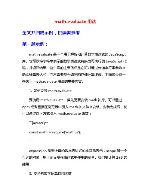
Seek simplicity, and distrust it.-Alfred North WhiteheadIn James R. Newman, The World of Mathematics, Vol. II,p. 1055, Tempus, WA: Redmond (1988).2 MATHEMATICALREPRESENTATIONS FOR COMPLEXDYNAMICS 2.1 Mathematical Representations and Theoretical ThinkingMeasurement cannot be separated from theory. Theoretical thinking is better through a mathematical representation. The choice of mathematical representations depends on the essential features in empirical observation and theoretical perspective. A mathematical representation should be powerful enough to display stylized features to be explained and simple enough to manage its mathematical solution to be solved. In the history of science, theoretical breakthrough often introduces radical changes in mathematical representation. For example, physicists once considered the Euclid geometry as an intrinsic nature of space. Einstein's work on gravitation theory offered a better alternative of a specific non-Euclid geometry in theoretical physics.Mathematical representation is an integrated part of theoretical thinking. New mathematical representations are introduced under new perspectives. Newtonian mechanics was developed by means of deterministic representation. Probability representation made its way through kinetic theory of gas, statistical mechanics, and quantum mechanics. The study of deterministic chaos in Hamiltonian and dissipative systems reveals a complementary relation between these two representations.There are different motives in choosing mathematical representation. For some scientists, the choice of mathematical representation is a choice of belief. Einstein refused the probability explanation of quantum mechanics because of his belief that God did not throw dice. Equilibrium economists reject economic chaos because of a fear that the existence of a deterministic pattern implies a failure of the perfect market. For some scientists, the issue of mathematical representation is a matter of taste and convenience. Hamiltonian formulation in theoretical economics has tremendous appeal because of its theoretical beauty and logical elegance. The discrete-time framework is dominated in econometrics because of its computational convenience in regression practice. For us, empirical relevance and theoretical generality are main drives in seeking new mathematical representations.30 Persistent Business CyclesThe equilibrium feature of economic movements is characterized by the Gaussian distribution with a finite mean and variance. The disequilibrium features can be described by a unimodal distribution deviated from the Gaussian distribution. During a bifurcation or transition process, a U-shaped or multimodal distribution may occur under nonequilibrium conditions. We will study the deterministic and probabilistic representations for equilibrium, disequilibrium, and nonequilibrium conditions.2.2 Trajectory and Probability Representation of Dynamical SystemsBoth trajectory and probability representation are mathematical abstractions of the real world. In physics, a trajectory of a planet is an abstraction and approximation when we ignore the size of the planet and its perturbation during movement. In biologic and social science, the trajectory representation can be perceived as an average behavior over repeated observations. The same procedure of averaging can be applied to the probability representation. The probability representation holds for large ensembles with identical properties.People may think that deterministic and stochastic approaches are conflicting representations. One strong argument in favor of stochastic modeling in economics is a human being's free will against determinism. However, this belief ignores a simple fact that these two representations coexist in theoretical literature. For example, the wave equation in quantum mechanics is a deterministic equation. However, its wave function has a probability interpretation. Traffic flow could be described by deterministic and stochastic models that were verified by extensive experiments (Prigogine and Herman 1971).For a given deterministic equation, we can have both trajectory representation and probability representation.The choice of mathematical representation depends on the question asked in your research. If your goal is forecasting a time path, you need the trajectory representation. If your interest is their average properties such as mean and variance, you need the probability representation.2.2.1 Time Averaging, Ensemble Averaging, and ErgocityTrajectory representation can be easily visualized by a time path of an observable such as a moving particle. Probability representation is more difficult because it contains more information.There are two approaches to introduce the concept of probability distribution. From a repeated experiment such as the case of coin tossing, a static approach can define a probability distribution as the average outcome. Probability represents the expectation from an event or experiment. A dynamic approach can construct a histogram from a time series. A dynamic probability distribution can be revealed from a histogram if the underlying dynamic is not changing over time. The question is does the time average represent the true possibility in future events.Mathematical Representations31 In statistical physics, the probability distribution is described in an ensemble that consists of a large number of identical systems. The probability distribution is considered as an average behavior of these identical systems. In mathematical literature, if the time averaging is equal to the ensemble averaging, this property is called ergocity. In mathematical economics, ergodic behavior is often assumed for stochastic models in time series analysis (Granger and Ter svirta 1993, Hamilton 1994). In statistical physics, it is hard to establish the ergotic behavior for physical systems. For example, non-ergotic behavior was found from the anharmonic oscillators in Hamiltonian systems (Reichl 1998). Contrary to previous belief, ergocity and the approach to equilibrium do not hold for most Hamiltonian systems. Chaos in Hamiltonian systems plays an important role in approaching equilibrium and ergocity. Almost all dynamic systems exhibit chaotic orbits. Nonlinearity and chaos appear to be the rule rather than exception in dynamical systems.Before discussing a probability distribution, we introduce the concept of a mean or average value μ which is a numerical measurement of the mathematical expectation E[x]. If there are N measurements of a variable X n , andN n ,...,2,1=, we haveμ =X X X NN12+++...(2.2.1a)For a probability distribution P x () where P x ()≥0 and P x dx ()=⎰1,we may have: E[x ] = μ = <>=⎰x xP x dx ()(2.2.1b)We also introduce the variance VAR[x ] and the standard deviation σ: VAR[x] = 22)(σμ>=-<x (2.2.2)In general, we can define a central moment about the mean:μμμn n n x x P x dx =<->=-⎰()()()(2.2.3)The most important distribution in probability theory is the Gaussian or normal distribution. A Gaussian distribution is completely determined by its first two moments: the mean μ and the standard deviation σ.32 Persistent Business CyclesFigure 2.1 Deterministic and probabilistic representation ofGaussian white noise.Mathematical Representations33 P x x ()(exp(())=--122222πσμσ (2.2.4)We may simply denote the Gaussian distribution as N (,)μσ.As a numerical example, the time path and histogram of the Gaussian random noise is shown in Figure 2.1.In principle, a stochastic system can be uniquely determined if its infinite moments are known. In empirical science, the critical issue is to determine the minimum moments for some characteristic behavior. In equilibrium statistical physics, the first two moments are good enough for many applications. In nonequilibrium statistical physics, higher moments may be needed. For example, the theory of non-Gaussian behavior in strong turbulence predicts up to the seventh moments observed in experiments. In economics, the first two to four moments are studied in empirical analysis.2.2.2 The Law of Large Numbers, The Central Limit Theorem, and Their BreakdownFor a large number of events, the Gaussian distribution provides a good description of its distribution. We have a set of N independent stochastic variables X 1, X 2, . . . X N with a common distribution. If their mean μ exist, the law of large numbers states that (Feller 1968):P X X X NN{|...|}120+++->→με(2.2.5)We denote its sum S N = X 1+X 2+ . . .+X N . Therefore, S N 抯 average (S N /N) approaches μ, and S N approaches N μ.If the first two moments exist for the above stochastic variables, the central limit theorem states that the probability distribution of S N approaches a Gaussian distribution with a mean of N μ and a standard deviation of N σ (van Kampen1992):P S N ()→ N (,)N N μσ(2.2.6)The Gaussian distribution is widely applied in statistics and econometrics because of the power of the law of large numbers and the central limit theorem. Therefore, the limitation of the Gaussian distribution can be seen when the law of large numbers and the central limit theorem break down.34 Persistent Business CyclesOne notable case is the non-existence of variance. For example, the Levy-Pareto distribution has infinite variance. The Levy distribution L(x) has an inverse power tail for large | x | (Montroll and Shlesinger 1984):L x x ()||()sin()()→-+12αααπΓ(2.2.7)where 0 < α < 2.When α = 1, the Levy distribution has a special case of the Cauchy distribution which has finite mean b but infinite variance (Feller 1968).)])[()(22a b x ax f +-=π (2.2.8)Empirical evidence of the Levy distribution is found in a broad distribution of commodity prices long-range correlations in turbulent flow (Mandelbrot 1963, Cootner 1964, Bouchaud and Georges 1990, Klafter, Shlesinger, and Zumofen 1996, Reichl 1998).Figure 2.2. Gaussian and Cauchy Distribution. The (0, 1) is the tallest in solid line. The Cauchy(1, 0) distribution is in the middle in dashed line, and Cauchy(π, 0) is the lowest and fattest distribution in dotted line.Mathematical Representations35 A comparison of the Cauchy distribution and the Gaussian distribution is shown in Figure 2.2. Both are unimodal distributions with zero mean. The variance of the standard Gaussian distribution is 1, and the variance of Cauchy distribution is infinite caused by its long tails.2.2.3 U-Shaped DistributionAnother interesting case is the U-shaped distribution such as the polarization in ferromagnetism and public opinion (Haken 1977, Chen 1991). For a U-shaped distribution, the concept of the expectation is meaningless, because the mean is the most unlikely event.In probability theory, there is a case of the arc sine law for a last visits that indicates a startling result in chance fluctuation (Feller 1968). Consider an ideal coin-tossing in 2n trials. The chances of tossing a head or a tail are equal. If the accumulated numbers of heads and tails are 2k. The probability is related to the following U-shaped distribution function:f x x x ()()=-11π(2.2.9)where x kn= and 0 < x < 1.Coin Tossing.36 Persistent Business CyclesIts probability distribution is shown in Figure 2.3. Its mean is 0.5. Its variance is 0.125. Its skewness is zero. Its kurtosis is 93. We must know that even the distribution of the sample mean approaches the Gaussian distribution, but the mean of the arc sine distribution represents the least likely event! This is a case that the central limit theorem is valid for a U-shaped distribution but the mean value may be quite misleading!People may think the most likely event should be anyone leading half the trial numbers. It is not! The most probable values for k are the extremes 0 and n. It is quite likely that in a long coin-tossing game, one of the players remains the whole time on the winning side, the other on the losing side. For example, in 20 tossings, the probability of leading 16 times or more is about 0.685; but the probability of leading 10 times is only 0.06! Therefore, the intuition of time averaging may lead to an erroneous picture of the probable effects of chance fluctuations. In other words, the expected value is misleading under a U-shaped distribution.2.2.4 Delta Function and Deterministic RepresentationDeterministic representation can be considered as a special case of probability representation when the probability distribution is a delta function. The delta function is very useful in quantum mechanics (Merzbacher 1970).0)'(=-x x δ when x x ≠' (2.2.10a)∞=)0(δ(2.2.10b)⎰∞∞-=1)(dx x δ(2.2.10c)⎰∞∞--=dx x x x f x f )'()()'(δ(2.2.10d)There are some useful properties for the delta function:)()(x x δδ=- (2.2.11a))()()()(a x a f a x x f -=-δδ(2.2.11b))(||1)(x a ax δδ=(2.2.11c) )]()([||1)()(b x a x b a b x a x -+--=--δδδδ(2.2.11d)Mathematical Representations37The delta function may have the following representations in terms of a limiting process (Merzbacher 1970, Stremler 1982):(a) A harmonic wave:⎰∞∞--=-ωωπδd x x i x x )}'(exp{21)'((2.2.11a)where i =-1.(b) A Gaussian pulse:}exp{lim )(22σπδσx x -=→(2.2.11b)(c) A two-sided exponential:}|2|exp{lim )(0σδσx x -=→(2.2.11c)(d) A Cauchy distribution pulse:)(lim1)(220σσπδσ+=→x x (2.2.11d)(e) A Sinc function:xx x )sin(lim1)(0σπδσ→=(2.2.11e)(f) A rectangular pulse function:)]2()2([1lim)(0εεεδε--+=→x u x u x (2.2.11f)where the unit step function is:u x x (')-=1 when x x ≥'u x x (')-=0 when x x <'(2.2.11g)38 Persistent Business Cycles(a)(b)Figure 2.4 The Relationship between Deterministic and ProbabilisticRepresentation. (a) A bifurcation tree of a deterministic system. (b) Thetrajectory and probability distribution representationIn economic dynamics, both a deterministic equation and a stochastic equation can be considered as an average description of a large number of systems. If the probability has a unimodal distribution, the time-path of its average position can be described by a trajectory.For a nonlinear deterministic system, bifurcation may occur like a bifurcation tree in Figure 2.4a. During a bifurcation point of a deterministic equation, theMathematical Representations39 corresponding probability distribution must have a polarized distribution as shown in Figure 2.4b.2.3 Linear Representations in the Time and Frequency DomainIn theoretical and empirical analysis, the time domain representation is applied in correlation analysis and the frequency domain representation is used in spectral analysis. They are useful tools for time series analysis for deterministic and stochastic systems.Theoretically, we can consider the spectral analysis as a representation in a functional space whose base function is harmonic waves, and the base function of correlation analysis is delta functions. Therefore, linear representations of a time series have only two building blocks: harmonic cycle and white noise. These two extreme models have a remarkable similarity: both of them can be described by delta functions. The image of a sine wave is a delta function in spectral space and the image of white noise is a delta function in correlation space.2.3.1 Time Domain Representation in Correlation AnalysisIt is very useful to introduce the concept of the covariance and the correlation for two functions of X(t) and Y(t):Cov X Y E X Y X Y [,][()()]=--μμ (2.3.1)Cor X Y Cov X Y X Y[,][,]=σσ (2.3.2)If X(t) and Y(t) are independent, their covariance and correlation are zero. We can also define the autocorrelation R(τ) of a function X(t):),()(ττ+=t t X X Cor R (2.3.3)We should note that correlation analysis is useful for stationary time series. For non-stationary time series, the time trend will introduce spurious correlations.For a Gaussian white noise ξi , its autocorrelation is a delta functionCor j k j k (,),ξξδ= (2.3.4)40 Persistent Business CyclesHere,δj k ,=0 when j k ≠ and δj j ,=1 when j k =.For a harmonic function )sin()(φω+=t A t X , its autocorrelation is a cosine function (Otnes and Enochson 1972)⎰-∞→++=2/2/)(*)(1lim),(T T T t t dt t X t X TX X Cor ττ= ⎰-∞→+++2/2/))(sin()sin(1lim T T T dt t t Tφτωφω= ⎰-∞→++-2/2/2)]22cos()[cos()2(1lim T T T dt t A T φωτωτω =⎰-∞→++-2/2/2)22cos(lim )cos(2T T T dt t A φτωωτω)2(cos 2)(cos 222τπτωPA A =⇒ (2.3.5)is white noise. The broken line is a sine wave with period P = 1.Here, the angular frequency Pf ππω22==, f is the frequency, and P the period. The phase informationφ is lost in the correlation function. The numericalexamples of a Gaussian white noise N (0,1) and a sine wave with period one isshown in Figure 2.5. Note: the autocorrelation of the sine wave decays slowlyMathematical Representations41 because of the finite time window T. We will discuss the role of the time window later.If we measure the time lag with the first zero-autocorrelation T o , it is near zero for white noise and 4Pfor a sine wave with period P.2.3.2 The Frequency Domain Representation in Spectral AnalysisIn a linear (vector) space, a vector x can be represented by a combination of n elementary vectors if the n elementary vectors consist of a complete set of orthogonal basis. Similarly, a function f t ()can be expanded in a functional space by a set of orthogonal and complete functions B t n () when t t t 12≤≤.x a b n n Nn ==∑1(2.3.6a)f t aB t nn n ()()==-∞∞∑(2.3.6b) ⎰=21)()(*)(1t t n nn dt t f t B t w a λ(2.3.6c)Here, w(t) is the weight function.There are many orthogonal polynomial functions in mathematical literature, such as the Hermite polynomials with a weight functione t -2, the Laguerre polynomialswith a weight function e t-, and the Lengendre polynomials with a unit weight function.Among all the orthogonal functions, the Fourier harmonic functions})({t n i n e t S ωω=or {)cos(),sin(t n t n ωω}plays an important role and havea wide range of applications. There are several reasons for its popularity in science literature. In physics, the harmonic oscillator, the plane waves in electromagnetic theory and quantum mechanics serve as the building blocks in classical and modern physics. In mathematics, harmonic functions are the basis for complex numbers and the theory of generalized functions. In information theory, harmonic signals can be transmitted in the most efficient way. The Fourier transform is defined by:42 Persistent Business Cycles⎰-==dt t i t f S t f F }exp{)(21)()]([ωπω(2.3.7a)and⎰==-ωωωπωd t i S t f S F }exp{)(21)()]([1(2.3.7b)The Levy distribution L(x) can be better described by its Fourier transform (Montroll and Shlesinger 1984):ωωωπαd a x i x L }||exp{21)(⎰∞∞---=(2.3.8)Here, 0 < α < 2. For the Gaussian distribution, α =2. For the Cauchy distribution, α = 1.2.3.3 The Power Spectrum and The Wiener-Khinchin Theorem The average power for f(t) is:⎰⎰∞∞-∞→-∞→==ωωπd S T dt t f Y T T T T 22/2/2|)(|211lim|)(|lim(2.3.9)Therefore, we have spectral densityG f ()ω:ωωπd G Y f )(21⎰∞∞-=(2.3.10)2|)(|1lim)(ωωS TG T f ∞→=(2.3.11)For a stationary time series with finite mean and variance, the time average is equal to its ensemble average, so that)()(*)()(*)(1limτττR t f t f dt t f t f T T >=-=<-⎰∞→(2.3.12)Then we have the Wiener-Khinchin Theorem (Reichl 1998):])([)exp{)()(τττωτωR F d i R G f =-=⎰(2.3.13)Mathematical Representations43For the Gaussian white noise, its correlation is a delta function, so its power spectrum is a constant:πδ21)]([=t F (2.3.14)For a harmonic oscillation, its correlation function is )cos(τω (see Equation (2.3.5)), its power spectrum is:)]'()'([22)]cos(2[22ωωδωωδπωτ-++=A A F(2.3.15)Therefore, we have two frequencies ±ω for a cosine correlation.For a correlation with a Gaussian wave packet, its power spectrum is still a Gaussian form. However, a fat bell curve will turn into a sharp one and vice versa.αωαα42221][--=e e F t(2.3.16)From the Wiener-Khinchin Theorem, we can see the correlation analysis and spectral analysis is closely related to each other, although they originated in the stochastic and deterministic approaches separately.2.4 Measures of the Deviations from the Gaussian DistributionAn equilibrium process is characterized by an unimodal distribution with finite variance. Long tails and long correlations indicate a deviation from equilibrium. For situations under far from equilibrium conditions, U-shaped and multimodal distributions are observed in natural and social phenomena (Chen 1987b, Wen, Chen, and Zhang 1996). Multimodal distribution may appear near a bifurcation point or in a transition regime. For example, option prices during the stock market crash have a bimodal distribution (Chen and Goodhart 1998).2.4.1 Locations of A Unimodal Distribution: the Mode, Mean, and Median44 Persistent Business CyclesIn addition to the arithmetic average, we have other useful measures of the central tendency of a distribution. The median X m is the value of the variate that divides the total frequency into two equal halves:⎰⎰∞-∞==mmX X dx x f dx x f 21)()( (2.4.1)The position of a local maximum in a probability distribution is called a mode X o . Similarly, we can define an antimode X a for a local minimum in distribution (Kendall 1987).For a Gaussian distribution, we have μ = X m =X o because of its symmetry. For a skew unimodal distribution, the mean, median, and mode are different.2.4.2 Deviations from Gaussian Distribution: Skewness and KurtosisCurrent statistics have several indicators of the deviation from Gaussian distribution. The deviation of a unimodal distribution from the Gaussian distribution is measured by their ratio of moments.For a Gaussian distribution, its symmetry is characterized by the fact that its odd moments are zero. For the even moments of a Gaussian distribution, we have:μ2n = !)!2(2)(22n n x nnnσμ>=-< (2.4.2)For N (0, 1 ), we have μ2 = 1, μ4 = 3.Therefore, the Gaussian distribution can serve as a benchmark in measuring the skewness 1β (the degree of distribution asymmetry) and the kurtosis 2β (the thickness of distribution tails). These can be done by comparing their third and forth moment in statistics (Kendall 1987, Greene 1993).1β=μσ33 (2.4.3)2β=344-σμ (2.4.4)For a positive1β, μ > X m > X o , and the upper tail of the unimodal distributionis heavier. For a negative1β, μ < X m < X o , and the lower tail is heavier.Mathematical Representations45 A distribution is called mesokurtic for 2β= 0, leptokurtic (thin) for2β> 0,and platykurtic (flat) for 2β< 0. For a Gaussian distribution, its 2βis zero.2.4.3 Information Entropy- A Measure of HomogeneityThe information entropy is a measure of homogeneity. It starts from a consideration of two-state distribution. Given the n discrete states (n = 1, 2, . . . , N) and their probability p n , the information entropy H is defined as the following (Shannon and Weaver 1949):H p p n n Nn =-=∑1log()(2.4.5) H H N ⇒=max log when p Nn =1(2.4.6)For N=2, we can set p p 1=and p q p 21==-. Therefore, we have:H p p p q q p p p p ()log log log ()log()=--=----110)1(log )(=-=ppp p H ∂∂when H p H ()max =.Therefore,H H p max ()log ===122(2.4.7)46 Persistent Business CyclesThe information entropy for two discrete states is shown in Figure 2.6.From the principle of maximum information entropy, we can find the corresponding distribution under a given condition (Goldman 1953). For a discrete distribution with a given mean m, the Poisson distribution has the maximum entropy.Let us consider the continuous distribution,⎰-=dxxpxpH)]([log)((2.4.8a)⎰=1)(dxxp(2.4.8b)Under the condition of a constant variance σ, the information entropy reaches the maximum when the distribution is a Gaussian.p x()=N2221),0(σπσσxe-=(2.4.9a)]2[log maxσπeH=(2.4.9b) and222)(σ=>=<⎰dxxpxx(2.4.9c)Mathematical Representations47 We can apply the Lagrange multipliers in the calculus of variations,dx p x dx p p H F ⎰⎰++=2)(βα01log 221=++--=x p pFλλ∂∂ when H H ⇒max (2.4.10)2211x e e p λλ-=(2.4.11)Substituting this value into Eq. (2.4.8b) and (2.4.9c) to determine λ1 and λ2, we get Eq.(2.4.9a).Similarly, we can find other distributions under different conditions. For example, under the condition of a constant mean μ, the distribution with maximum entropy is:μμxex p -=1)( (2.4.12a))(log max μe H =(2.4.12b)when 0)(>=>=<⎰μdx x p x x(2.4.12c)Under the condition of limited peak range, say the range of ||x S 2≤p x S()=12(2.4.13a)H S max log()=124 (2.4.13b)⎰-=SSdx x p 1)((2.4.13c)You can prove that: under constant information entropy H, the Gaussian distribution has the smallest variance among any one-dimensional probability distribution.48 Persistent Business CyclesThe meaning of information entropy is sometimes confusing, since information has different implications under different situations. For example, the concept of average measures the central tendency of a distribution, the variance measures the range of the central tendency, and the information entropy measures the homogeneity of a distribution. The principle of maximum entropy indicates the tendency towards a homogeneous state without any structure.There is a close relation between thermodynamic entropy in equilibrium statistical mechanics and information entropy in information theory. However, there is difficulty in defining entropy in nonequilibrium statistical mechanics (Penrose 1979). Correlation and non-Markovian property make the description of an open system much more complex than a closed or isolated system.From the perspective of nonequilibrium physics, economies are open systems with expanding energy sources. The Gaussian distribution may appear in an isolated system with the conservation of energy or in a closed system with a stable environment. Under continuing flows of energy and negative entropy, probability distributions in open economies will significantly deviate from the Gaussian distribution. Observed deviations from a Gaussian distribution can serve as a measure of out-of-equilibrium in real economies.The following factors may create nonequilibrium conditions: a finite number of economic players (such as the dominance of large firms), a finite range of variables (such as the credit ceiling and resource limitations), long-range correlations (such as credit history and social relations), and nonlinear interactions (such as overshooting and positive feedback in economic control), etc. The statistics of skewness and kurtosis provide some quantitative measure of the degree of out-of equilibrium. The most serious case is the Levy distribution with infinite variance. So far the discussion in this section is based on the stable distributions that are unimodal. As far as we know, there is no theoretical foundation to restrict economic study to unimodal distributions. Empirical observations of economic instabilities need a broader scope in mathematical modeling.2.4.4 Polarization and Unpredictable Uncertainty- Multimodal and U-Shaped DistributionA Partial deviation from the central tendency can be measured by deviations from a Gaussian distribution. A radical deviation from the central tendency cannot be well described by any unimodal distribution. Multimodal distribution is observed in the far-from-equilibrium situations such as the cases of rapid chemical reactions and the transition period in a multi-staged growth (Chen 1987b). The bimodal and U-shaped distribution is discussed in critical phenomena such as ferromagnetism and fashion model of public opinion (Haken 1977, Chen 1991). The bimodal distribution is also observed in stock price changes and in option prices (Osborne 1959, Jackwerth and Rubinstein 1996).The interest in bimodal and multimodal distribution mainly comes from studies of time evolution problems. The origin of the probability theory is static theory of。