Optimal and suboptimal singleton arc consistency algorithms

基于遗传算法的两通道完全重构滤波器组的设计
徐华楠;刘哲
【期刊名称】《微电子学与计算机》
【年(卷),期】2008(25)3
【摘要】介绍了两通道滤波器组的完全重构条件,利用Euclidean分解算法,将两通道滤波器组的设计问题简化为寻找给定特性的低通滤波器的最佳Euclidean互补滤波器的单变量非线性优化问题,并探讨了采用遗传算法设计此类高度非线性优化问题.最后通过设计例子说明将遗传算法应用到滤波器组的设计中是可行的.
【总页数】5页(P144-148)
【关键词】两通道滤波器组;遗传算法;完全重构;因式分解
【作者】徐华楠;刘哲
【作者单位】西北工业大学理学院
【正文语种】中文
【中图分类】TP31
【相关文献】
1.两通道完全重构滤波器组的设计方法:因式分解法 [J], 石光明;焦李成
2.无完全重构约束的两通道自适应FIR滤波器组设计 [J], 王兰美;水鹏朗;廖桂生;王桂宝
3.基于多项式分解理论的低时延完全重构两通道滤波器组的设计 [J], 石光明;焦李成
4.基于进化计算设计无乘法的完全重构两通道滤波器组 [J], 石光明;张子敬;焦李成
5.两通道完全重构全相位FIR滤波器组的设计 [J], 黄翔东;王兆华
因版权原因，仅展示原文概要，查看原文内容请购买。

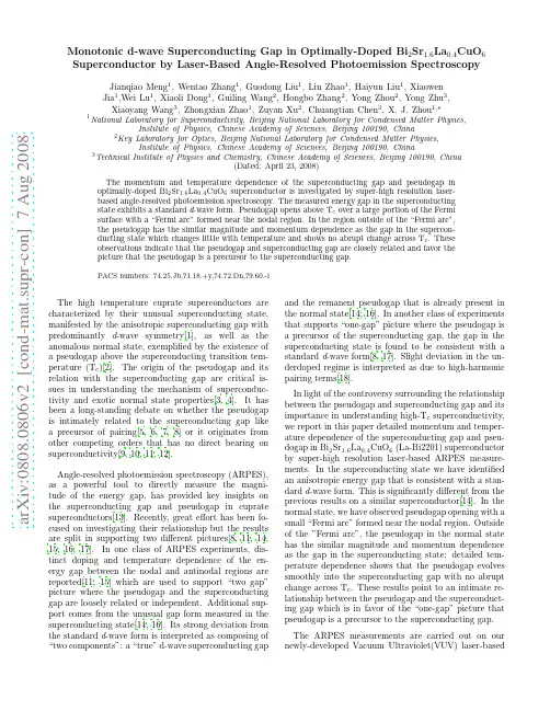
a r X i v :0808.0806v 2 [c o n d -m a t .s u p r -c o n ] 7 A u g 2008Monotonic d-wave Superconducting Gap in Optimally-Doped Bi 2Sr 1.6La 0.4CuO 6Superconductor by Laser-Based Angle-Resolved Photoemission SpectroscopyJianqiao Meng 1,Wentao Zhang 1,Guodong Liu 1,Lin Zhao 1,Haiyun Liu 1,Xiaowen Jia 1,Wei Lu 1,Xiaoli Dong 1,Guiling Wang 2,Hongbo Zhang 2,Yong Zhou 2,Yong Zhu 3,Xiaoyang Wang 3,Zhongxian Zhao 1,Zuyan Xu 2,Chuangtian Chen 3,X.J.Zhou 1,∗1National Laboratory for Superconductivity,Beijing National Laboratory for Condensed Matter Physics,Institute of Physics,Chinese Academy of Sciences,Beijing 100190,China2Key Laboratory for Optics,Beijing National Laboratory for Condensed Matter Physics,Institute of Physics,Chinese Academy of Sciences,Beijing 100190,China3Technical Institute of Physics and Chemistry,Chinese Academy of Sciences,Beijing 100190,China(Dated:April 23,2008)The momentum and temperature dependence of the superconducting gap and pseudogap in optimally-doped Bi 2Sr 1.6La 0.4CuO 6superconductor is investigated by super-high resolution laser-based angle-resolved photoemission spectroscopy.The measured energy gap in the superconducting state exhibits a standard d -wave form.Pseudogap opens above T c over a large portion of the Fermi surface with a “Fermi arc”formed near the nodal region.In the region outside of the “Fermi arc”,the pseudogap has the similar magnitude and momentum dependence as the gap in the supercon-ducting state which changes little with temperature and shows no abrupt change across T c .These observations indicate that the pseudogap and superconducting gap are closely related and favor the picture that the pseudogap is a precursor to the superconducting gap.PACS numbers:74.25.Jb,71.18.+y,74.72.Dn,79.60.-iThe high temperature cuprate superconductors are characterized by their unusual superconducting state,manifested by the anisotropic superconducting gap with predominantly d -wave symmetry[1],as well as the anomalous normal state,exemplified by the existence of a pseudogap above the superconducting transition tem-perature (T c )[2].The origin of the pseudogap and its relation with the superconducting gap are critical is-sues in understanding the mechanism of superconduc-tivity and exotic normal state properties[3,4].It has been a long-standing debate on whether the pseudogap is intimately related to the superconducting gap like a precursor of pairing[5,6,7,8]or it originates from other competing orders that has no direct bearing on superconductivity[9,10,11,12].Angle-resolved photoemission spectroscopy (ARPES),as a powerful tool to directly measure the magni-tude of the energy gap,has provided key insights on the superconducting gap and pseudogap in cuprate superconductors[13].Recently,great effort has been fo-cused on investigating their relationship but the results are split in supporting two different pictures[8,11,14,15,16,17].In one class of ARPES experiments,dis-tinct doping and temperature dependence of the en-ergy gap between the nodal and antinodal regions are reported[11,15]which are used to support “two gap”picture where the pseudogap and the superconducting gap are loosely related or independent.Additional sup-port comes from the unusual gap form measured in the superconducting state[14,16].Its strong deviation from the standard d -wave form is interpreted as composing of “two components”:a “true”d-wave superconducting gapand the remanent pseudogap that is already present in the normal state[14,16].In another class of experiments that supports “one-gap”picture where the pseudogap is a precursor of the superconducting gap,the gap in the superconducting state is found to be consistent with a standard d -wave form[8,17].Slight deviation in the un-derdoped regime is interpreted as due to high-harmonic pairing terms[18].In light of the controversy surrounding the relationship between the pseudogap and superconducting gap and its importance in understanding high-T c superconductivity,we report in this paper detailed momentum and temper-ature dependence of the superconducting gap and pseu-dogap in Bi 2Sr 1.6La 0.4CuO 6(La-Bi2201)superconductor by super-high resolution laser-based ARPES measure-ments.In the superconducting state we have identified an anisotropic energy gap that is consistent with a stan-dard d -wave form.This is significantly different from the previous results on a similar superconductor[14].In the normal state,we have observed pseudogap opening with a small “Fermi arc”formed near the nodal region.Outside of the ”Fermi arc”,the pseudogap in the normal state has the similar magnitude and momentum dependence as the gap in the superconducting state:detailed tem-perature dependence shows that the pseudogap evolves smoothly into the superconducting gap with no abrupt change across T c .These results point to an intimate re-lationship between the pseudogap and the superconduct-ing gap which is in favor of the “one-gap”picture that pseudogap is a precursor to the superconducting gap.The ARPES measurements are carried out on our newly-developed Vacuum Ultraviolet(VUV)laser-based2E - EF (eV)E - EF (eV)1.00.50G (0,0)(p ,0)1510152025k xFIG.1:Fermi surface of the optimally-doped La-Bi2201(T c =32K)and corresponding photoemission spectra (EDCs)on the Fermi surface at various temperatures.(a).Spectral weight as a function of two-dimensional momentum (k x ,k y )integrated over [-5meV,5meV]energy window with respect to the Fermi level E F .The measured Fermi momenta are marked by red empty circles and labeled by numbers;(b).Original EDCs along the Fermi surface measured at 15K.The symmetrized EDCs along the Fermi surface are shown in (c)for 15K,(d)for 25K and (e and f)for 40K.The numbers on panels (b-f)corresponds to the Fermi momentum numbers in (a).angle-resolved photoemission system with advantages of super-high energy resolution,high momentum resolution,high photon flux and enhanced bulk sensitivity[19].The photon energy is 6.994eV with a bandwidth of 0.26meV and the energy resolution of the electron energy analyzer (Scienta R4000)was set at 0.5meV,giving rise to an overall energy resolution of 0.56meV.The angular res-olution is ∼0.3◦,corresponding to a momentum resolu-tion ∼0.004˚A −1at the photon energy of 6.994eV.The optimally doped Bi 2Sr 2−x La x CuO 6(La-Bi2201)(x=0.4,T c ∼32K,transition width ∼2K)single crystals were grown by the traveling solvent floating zone method[20].One advantage of choosing La-Bi2201system lies in its relatively low superconducting transition temperature that is desirable in investigating the normal state behav-ior with suppressed thermal broadening of photoemission spectra.The samples are cleaved in situ in vacuum with a base pressure better than 4×10−11Torr.Fig.1(a)shows the Fermi surface mapping of the op-timally doped La-Bi2201(T c =32K)measured at 15K.The low photon energy and high photon flux have made it possible to take dense sampling of the measurements in the momentum space.The photoemission spectra (En-ergy Distribution Curves,EDCs)along the Fermi surface are plotted in Fig.1(b).The EDCs near the nodal re-gion show sharp peaks that are similar to those observed in Bi2212[21].When the momentum moves away from the nodal region to the (0,π)antinodal region,the EDC peaks get weaker,but peak feature remains along the en-tire Fermi surface even for the one close to the antinodal region.The EDC peak position also shifts away from the Fermi level when the momentum moves from the nodal to the antinodal region,indicating a gap opening in the superconducting state.Note that the EDCs near the antinodal region do not show any feature near 40meV that was reported in a previous measurement[14].In order to extract the energy gap,we have sym-metrized the original EDCs with respect to the Fermi level,as shown in Fig.1c for the 15K measurements,and Fig.1d and Fig.1(e-f)for 25K and 40K,respec-tively.The symmetrization procedure not only provides an intuitive way in visualizing the energy gap,but also removes the effect of Fermi cutoffin photoemission spec-tra and provides a quantitative way in extracting the gap size[22].The symmetrized EDCs have been fitted using the general phenomenological form[22];the fitted curves are overlaid in Fig.1(c-f)and the extracted gap size is plotted in Fig.2.As shown in Fig.2,the gap in the superconducting state exhibits a clear anisotropic behavior that is consis-tent with a standard d -wave form ∆=∆0cos(2Φ)(or in a more strict sense,∆=∆0|cos (k x a )−cos (k y a )|/2form as shown in the inset of Fig.2)with a maximum energy gap ∆0=15.5meV.It is also interesting to note that the gap is nearly identical for the 15K and 25K measurements for such a T c =32K superconductor.These results are significantly different from a recent measurement where the gap in the superconducting state deviates strongly from the standard d -wave form with an antinodal gap at 40meV[14].An earlier measurement[23]gave an antin-3G a p S i z e (m e V )Angle F (degrees)FIG.2:Energy gap along the Fermi surface measured at 15K (solid circles),25K (empty circles)and 40K (empty squares)on the optimally-doped La-Bi2201(T c =32K).The solid red line is fitted from the measured data at 15K which gives ∆=15.5cos(2Φ).The Φangle is defined as shown in the bottom-right inset.The upper-right inset shows the gap size as a function of |cos (k x a )−cos (k y a )|/2at 15K and 25K.The pink line represents a fitted line with ∆=15.5|cos (k x a )−cos (k y a )|/2.odal gap at 10∼12meV which is close to our present mea-surement,but it also reported strong deviation from the standard d -wave form.While the non-d -wave energy gap can be interpreted ascomposed of two components in the previous measurement[14],our present results clearly in-dicate that the gap in the superconducting state is dom-inated by a d -wave component.In the normal state above T c =32K,the Fermi sur-face measured at 40K is still gapped over a large portion except for the section near the nodal region that shows a zero gap,as seen from the symmetrized EDCs (Fig.1e-f for 40K)and the extracted pseudo-gap (40K data in Fig.2).This is consistent with the “Fermi arc”picture observed in other high temperature superconductors[6,11,24].Note that the pseudogap out-side of the “Fermi arc”region shows similar magnitude and momentum dependence as the gap in the supercon-ducting state (Fig.2).Fig.3shows detailed temperature dependence of EDCs and the associated energy gap for two representa-tive momenta on the Fermi surface.Strong temperature dependence of the EDCs is observed for the Fermi mo-mentum A (Fig.3a).At high temperatures like 100K or above,the EDCs show a broad hump structure near -0.2eV with no observable peak near the Fermi level.Upon cooling,the high-energy -0.2eV broad hump shows little change with temperature,while a new structure emerges near the Fermi level and develops into a sharp “quasipar-ticle”peak in the superconducting state,giving rise to a peak-dip-hump structure in EDCs.This temperatureE - EF (eV)E - EF (eV)FIG.3:(a,b).Temperature dependence of representa-tive EDCs at two Fermi momenta on the Fermi surface in optimally-doped La-Bi2201.The location of the Fermi mo-menta is indicated in the inset.Detailed temperature depen-dence of the symmetrized EDCs for the Fermi momentum A are shown in (c)and for the Fermi momentum B in (d).The dashed lines in (c)and (d)serve as a guide to the eye.evolution and peak-dip-hump structure are reminiscent to that observed in other high temperature superconduc-tors like Bi2212[25].When moving towards the antin-odal region,as for the Fermi momentum B (Fig.3b),the EDCs qualitatively show similar behavior although the temperature effect gets much weaker.One can still see a weak peak developed at low temperatures,e.g.,13K,near the Fermi level.To examine the evolution of the energy gap with tem-perature,Fig.3c and 3d show symmetrized EDCs mea-sured at different temperatures for the Fermi momenta A and B,respectively.The gap size extracted by fit-ting the symmetrized EDCs with the general formula[22]are plotted in Fig. 4.For the Fermi momentum A,as seen from Fig.3c,signature of gap opening in the su-perconducting state persists above T c =32K,remaining obvious at 50K,getting less clear at 75K,and appear to disappear around 100K and above as evidenced by the appearance of a broad peak.The gap size below 50K (Fig.4)shows little change with temperature and no abrupt change is observed across T c .The data at 75K is hard to fit to get a reliable gap size,thus not included in Fig. 4.When the momentum moves closer to the antinodal region,as for the Fermi momentum B,simi-lar behaviors are observed,i.e.,below 50K,the gap size is nearly a constant without an abrupt change near T c .But in this case,different from the Fermi momentum A,4G a p S i z e (m e V )Temperature(K)FIG.4:Temperature dependence of the energy gap for two Fermi momenta A (empty squares)and B (empty circles)as indicated in insets of Fig.3(a)and (b),and also indicated in the up-right inset,for optimally-doped La-Bi2201.The dashed line indicates T c =32K.there is no broad peak recovered above 100K,probably indicating a higher pseudogap temperature.This is qual-itatively consistent with the transport[26]and NMR[27]measurements on the same material that give a pseudo-gap temperature between 100∼150K.From precise gap measurement,there are clear signa-tures that can distinct between “one-gap”and “two-gap”scenarios[4].In the “two-gap”picture where the pseudo-gap and superconducting gap are assumed independent,because the superconducting gap opens below T c in addi-tion to the pseudogap that already opens in the normal state and persists into the superconducting state,one would expect to observe two effects:(1).Deviation of the energy gap from a standard d -wave form in the super-conducting state with a possible break in the measured gap form[14];(2).Outside of the “Fermi arc”region,one should expect to see an increase in gap size in the superconducting state.Our observations of standard d -wave form in the superconducting state (Fig.2),similar magnitude and momentum dependence of the pseudogap and the gap in the superconducting state outside of the “Fermi arc”region (Fig.2),smooth evolution of the gap size across T c and no indication of gap size increase upon entering the superconducting state (Fig.4),are not com-patible with the expectations of the “two-gap”picture.They favor the “one-gap”picture where the pseudogap and superconducting gap are closely related and the pseu-dogap transforms into the superconducting gap across T c .Note that,although the region outside of the “Fermi arc”shows little change of the gap size with temperature (Fig.4),the EDCs exhibit strong temperature depen-dence with a “quasiparticle”peak developed in the su-perconducting state(Fig.3a and 3b)that can be related with the establishment of phase coherence[8,25].This suggests that the pseudogap region on the Fermi surface can sense the occurrence of superconductivity through acquiring phase coherence.In conclusion,from our precise measurements on the detailed momentum and temperature dependence of the energy gap in optimally doped La-Bi2201,we provide clear evidence to show that the pseudogap and super-conducting gap are intimately related.Our observations are in favor of the “one-gap”picture that the pseudogap is a precursor to the superconducting gap and supercon-ductivity is realized by establishing a phase coherence.We acknowledge helpful discussions with T.Xi-ang.This work is supported by the NSFC(10525417and 10734120),the MOST of China (973project No:2006CB601002,2006CB921302),and CAS (Projects IT-SNEM and 100-Talent).∗Corresponding author:XJZhou@[1]See,e.g.,C.C.Tsuei and J.R.Kirtley,Rev.Mod.Phys.72,969(2000).[2]T.Timusk and B.Statt,Rep.Prog.Phys.62,61(1999).[3]V.J.Emery and S.A.Kivelson,Nature (London)374,434(1995);X.G.Wen and P.A.Lee,Phys.Rev.Lett.76,503(1996);C.M.Varma,Phys.Rev.Lett.83,3538(1999);S.Chakravarty et al.,Phys.Rev.B 63,094503(2001);P.W.Anderson,Phys.Rev.Lett.96,017001(2006).[4]lis,Science 314,1888(2006).[5]Ch.Renner et al.,Phys.Rev.Lett.80,149(1998).[6]M.R.Norman et al.,Nature (London)392,157(1998).[7]Y.Y.Wang et al.,Phys.Rev.B 73,024510(2006).[8]A.Kanigel et al.,Phys.Rev.Lett.99,157001(2007).[9]G.Deytscher,Nature (London)397,410(1999).[10]M.Le.Tacon et al.,Nature Phys.2,537(2006).[11]K.Tanaka et al.,Scinece 314,1910(2006).[12]M.C.Boyer et al.,Nature Phys.3,802(2007).[13]A.Damascelli et al.,Rev.Mod.Phys.75,473(2003);J.C.Campuzano et al.,in The Physics of Superconductors,Vol.2,edited by K.H.Bennemann and J.B.Ketterson,(Springer,2004).[14]T.Kondo et al.,Phys.Rev.Lett.98,267004(2007).[15]W.S.Lee et al.,Nature (London)450,81(2007).[16]K.Terashima et al.,Phys.Rev.Lett.99,017003(2007).[17]M.Shi et al.,arXiv:cond-mat/0708.2333.[18]J.Mesot et al.,Phys.Rev.Lett.83,840(1999).[19]G.D Liu et al.,Rev.Sci.Instruments 79,023105(2008).[20]J.Q.Meng et al.,unpublished work.[21]W.T.Zhang et al.,arXiv:cond-mat/0801.2824.[22]M.R.Norman et al.,Phys.Rev.B 57,R11093(1998).[23]J.M.Harris et al.,Phys.Rev.Lett.79,143(1997).[24]A.Kanigel et al.,Nature Phys.2447(2006).[25]A.V.Fedorov et al.,Phys.Rev.Lett.82,2179(1999);D.L.Feng et al.,Science 289,277(2000);H.Ding et al.,Phys.Rev.Lett.87,227001(2001).[26]Y.Ando et al.,Phys.Rev.Lett.93,267001(2004).[27]G.-Q.Zheng et al.,Phys.Rev.Lett.94,047006(2005).。

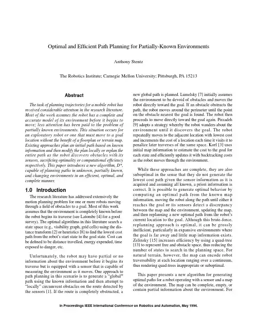
Optimal and Efficient Path Planning for Partially-Known EnvironmentsAnthony StentzThe Robotics Institute; Carnegie Mellon University; Pittsburgh, PA 15213AbstractThe task of planning trajectories for a mobile robot has received considerable attention in the research literature. Most of the work assumes the robot has a complete and accurate model of its environment before it begins to move; less attention has been paid to the problem of partially known environments. This situation occurs for an exploratory robot or one that must move to a goal location without the benefit of a floorplan or terrain map. Existing approaches plan an initial path based on known information and then modify the plan locally or replan the entire path as the robot discovers obstacles with its sensors, sacrificing optimality or computational efficiency respectively. This paper introduces a new algorithm, D*, capable of planning paths in unknown, partially known, and changing environments in an efficient, optimal, and complete manner.1.0IntroductionThe research literature has addressed extensively the motion planning problem for one or more robots moving through a field of obstacles to a goal. Most of this work assumes that the environment is completely known before the robot begins its traverse (see Latombe [4] for a good survey). The optimal algorithms in this literature search a state space (e.g., visibility graph, grid cells) using the dis-tance transform [2] or heuristics [8] to find the lowest cost path from the robot’s start state to the goal state. Cost can be defined to be distance travelled, energy expended, time exposed to danger, etc.Unfortunately, the robot may have partial or no information about the environment before it begins its traverse but is equipped with a sensor that is capable of measuring the environment as it moves. One approach to path planning in this scenario is to generate a “global”path using the known information and then attempt to “locally” circumvent obstacles on the route detected by the sensors [1]. If the route is completely obstructed, a new global path is planned. Lumelsky [7] initially assumes the environment to be devoid of obstacles and moves the robot directly toward the goal. If an obstacle obstructs the path, the robot moves around the perimeter until the point on the obstacle nearest the goal is found. The robot then proceeds to move directly toward the goal again. Pirzadeh [9] adopts a strategy whereby the robot wanders about the environment until it discovers the goal. The robot repeatedly moves to the adjacent location with lowest cost and increments the cost of a location each time it visits it to penalize later traverses of the same space. Korf [3] uses initial map information to estimate the cost to the goal for each state and efficiently updates it with backtracking costs as the robot moves through the environment.While these approaches are complete, they are also suboptimal in the sense that they do not generate the lowest cost path given the sensor information as it is acquired and assuming all known, a priori information is correct. It is possible to generate optimal behavior by computing an optimal path from the known map information, moving the robot along the path until either it reaches the goal or its sensors detect a discrepancy between the map and the environment, updating the map, and then replanning a new optimal path from the robot’s current location to the goal. Although this brute-force, replanning approach is optimal, it can be grossly inefficient, particularly in expansive environments where the goal is far away and little map information exists. Zelinsky [15] increases efficiency by using a quad-tree [13] to represent free and obstacle space, thus reducing the number of states to search in the planning space. For natural terrain, however, the map can encode robot traversability at each location ranging over a continuum, thus rendering quad-trees inappropriate or suboptimal.This paper presents a new algorithm for generating optimal paths for a robot operating with a sensor and a map of the environment. The map can be complete, empty, or contain partial information about the environment. ForIn Proceedings IEEE International Conference on Robotics and Automation, May 1994.regions of the environment that are unknown, the map may contain approximate information, stochastic models for occupancy, or even a heuristic estimates. The algorithm is functionally equivalent to the brute-force,optimal replanner, but it is far more efficient.The algorithm is formulated in terms of an optimal find-path problem within a directed graph, where the arcs are labelled with cost values that can range over a continuum. The robot’s sensor is able to measure arc costs in the vicinity of the robot, and the known and estimated arc values comprise the map. Thus, the algorithm can be used for any planning representation, including visibility graphs [5] and grid cell structures. The paper describes the algorithm, illustrates its operation, presents informal proofs of its soundness, optimality, and completeness, and then concludes with an empirical comparison of the algorithm to the optimal replanner.2.0The D* AlgorithmThe name of the algorithm, D*, was chosen because it resembles A* [8], except that it is dynamic in the sense that arc cost parameters can change during the problem-solving process. Provided that robot motion is properly coupled to the algorithm, D* generates optimal trajecto-ries. This section begins with the definitions and notation used in the algorithm, presents the D* algorithm, and closes with an illustration of its operation.2.1DefinitionsThe objective of a path planner is to move the robot from some location in the world to a goal location, such that it avoids all obstacles and minimizes a positive cost metric (e.g., length of the traverse). The problem space can be formulated as a set of states denoting robot loca-tions connected by directional arcs , each of which has an associated cost. The robot starts at a particular state and moves across arcs (incurring the cost of traversal) to other states until it reaches the goal state, denoted by . Every state except has a backpointer to a next state denoted by . D* uses backpointers to represent paths to the goal. The cost of traversing an arc from state to state is a positive number given by the arc cost function . If does not have an arc to , then is undefined. Two states and are neighbors in the space if or is defined.Like A*, D* maintains an list of states. The list is used to propagate information about changes to the arc cost function and to calculate path costs to states in the space. Every state has an associated tag ,such that if has never been on the list, if is currently on the list, andG X G Y b X ()Y =Y X c X Y ,()Y X c X Y ,()X Y c X Y ,()c Y X ,()OPEN OPEN X t X ()t X ()NEW =X OPEN t X ()OPEN =XOPEN if is no longer on the list. For each state , D* maintains an estimate of the sum of the arc costs from to given by the path cost function . Given the proper conditions, this estimate is equivalent to the optimal (minimal) cost from state to , given by the implicit function . For each state on the list (i.e.,), the key function,, is defined to be equal to the minimum of before modification and all values assumed by since was placed on the list. The key function classifies a state on the list into one of two types:a state if , and a state if . D* uses states on the listto propagate information about path cost increases (e.g.,due to an increased arc cost) and states to propagate information about path cost reductions (e.g.,due to a reduced arc cost or new path to the goal). The propagation takes place through the repeated removal of states from the list. Each time a state is removed from the list, it is expanded to pass cost changes to its neighbors. These neighbors are in turn placed on the list to continue the process.States on the list are sorted by their key function value. The parameter is defined to be for all such that . The parameter represents an important threshold in D*: path costs less than or equal to are optimal, and those greater than may not be optimal. The parameter is defined to be equal to prior to most recent removal of a state from the list. If no states have been removed,is undefined.An ordering of states denoted by is defined to be a sequence if for all such that and for all such that . Thus, a sequence defines a path of backpointers from to . A sequence is defined to be monotonic if( a n d) o r ( and ) for all such that . D* constructs and maintains a monotonic sequence , representing decreasing current or lower-bounded path costs, for each state that is or was on the list. Given a sequence of states , state is an ancestor of state if and a descendant of if .For all two-state functions involving the goal state, the following shorthand notation is used:.Likewise, for sequences the notation is used.The notation is used to refer to a function independent of its domain.t X ()CLOSED =X OPEN X X G h G X ,()X G o G X ,()X OPEN t X ()OPEN =k G X ,()h G X ,()h G X ,()X OPEN X OPEN RAISE k G X ,()h G X ,()<LOWER k G X ,()h G X ,()=RAISE OPEN LOWER OPEN OPEN OPEN k min min k X ()()X t X ()OPEN =k min k min k min k old k min OPEN k old X 1X N {,}b X i 1+()X i =i 1i ≤N <X i X j ≠i j (,)1i ≤j <N ≤X N X 1X 1X N {,}t X i ()CLOSED =h G X i ,()h G X i 1+,()<t X i ()OPEN =k G X i ,()h G X i 1+,()<i 1i ≤N <G X {,}X OPEN X 1X N {,}X i X j 1i j N ≤<≤X j 1j i N ≤<≤f X ()f G X ,()≡X {}G X {,}≡f °()2.2Algorithm DescriptionThe D* algorithm consists primarily of two functions: and .is used to compute optimal path costs to the goal, and is used to change the arc cost function and enter affected states on the list. Initially, is set to for all states,is set to zero, and is placed on the list. The first function,, is repeatedly called until the robot’s state,, is removed from the list (i.e.,) or a value of -1 is returned, at which point either the sequence has been computed or does not exist respectively. The robot then proceeds to follow the backpointers in the sequence until it eitherreaches the goal or discovers an error in the arc cost func-tion (e.g., due to a detected obstacle). The second function,, is immediately called to cor-rect and place affected states on the list. Let be the robot’s state at which it discovers an error in .By calling until it returns ,the cost changes are propagated to state such that . At this point, a possibly new sequence has been constructed, and the robot continues to follow the backpointers in the sequence toward the goal.T h e a l g o r i t h m s f o r a n d are presented below. The embedded routines are , which returns the state on the list with minimum value ( if the list is empty);, which returns for the list (-1 if the list is empty);, which deletes state from the list and sets ; and , w h i c h c o m p u t e s i f , if , and i f , s e t s and , and places or re-positions state on the list sorted by .In function at lines L1 through L3,the state with the lowest value is removed from the list. If is a state (i.e.,), its path cost is optimal since is equal to the old . At lines L8 through L13, each neighbor of is examined to see if its path cost can be lowered. Additionally,neighbor states that are receive an initial path cost value, and cost changes are propagated to each neighbor that has a backpointer to , regardless of whether the new cost is greater than or less than the old. Since these states are descendants of , any change to the path cost of affects their path costs as well. The backpointer of is redirected (if needed) so that the monotonic sequence is constructed. All neighbors that receive a new pathPROCESS STATE –MODIFY COST –PROCESS STATE –MODIFY COST –c °()OPEN t °()NEW h G ()G OPEN PROCESS STATE –X OPEN t X ()CLOSED =X {}X {}c °()MODIFY COST –c °()OPEN Y c °()PROCESS STATE –k min h Y ()≥Y h Y ()o Y ()=Y {}PROCESS STATE –MODIFY COST –MIN STATE –OPEN k °()NULL GET KMIN –k min OPEN DELETE X ()X OPEN t X ()CLOSED =INSERT X h new ,()k X ()h new =t X ()NEW =k X ()min k X ()h new ,()=t X ()OPEN =k X ()min h X ()h new ,()=t X ()CLOSED =h X ()h new =t X ()OPEN =X OPEN k °()PROCESS STATE –X k °()OPEN X LOWER k X ()h X ()=h X ()k min Y X NEW Y X X X Y Y {}cost are placed on the list, so that they will propagate the cost changes to their neighbors.If is a state, its path cost may not be optimal.Before propagates cost changes to its neighbors, its optimal neighbors are examined at lines L4 through L7 to see if can be reduced. At lines L15 through L18, cost changes are propagated to states and immediate descendants in the same way as for states. If is able to lower the path cost of a state that is not an immediate descendant (lines L20 and L21), is placed back on the list for future expansion. It is shown in the next section that this action is required to avoid creating a closed loop in the backpointers. If the path cost of is able to be reduced by a suboptimal neighbor (lines L23 through L25), the neighbor is placed back on the list. Thus, the update is “postponed” until the neighbor has an optimal path cost.Function: PROCESS-STATE ()L1L2if then return L3;L4if then L5for each neighbor of :L6if and then L7;L8if then L9for each neighbor of :L10if or L11( and ) or L12( and ) then L13;L14else L15for each neighbor of :L16if or L17( and ) then L18;L19else L20if and then L21L22else L23if and and L24 and then L25L26return OPEN X RAISE X h X ()NEW LOWER X X OPEN X OPEN X MIN STATE ()–=X NULL =1–k old GET KMIN –()=DELETE X ()k old h X ()<Y X h Y ()k old ≤h X ()h Y ()c Y X ,()+>b X ()Y =h X ()h Y ()c Y X ,()+=k old h X ()=Y X t Y ()NEW =b Y ()X =h Y ()h X ()c X Y ,()+≠b Y ()X ≠h Y ()h X ()c X Y ,()+>b Y ()X =INSERT Y h X ()c X Y ,()+,()Y X t Y ()NEW =b Y ()X =h Y ()h X ()c X Y ,()+≠b Y ()X =INSERT Y h X ()c X Y ,()+,()b Y ()X ≠h Y ()h X ()c X Y ,()+>INSERT X h X (),()b Y ()X ≠h X ()h Y ()c Y X ,()+>t Y ()CLOSED =h Y ()k old >INSERT Y h Y (),()GET KMIN ()–In function , the arc cost function is updated with the changed value. Since the path cost for state will change, is placed on the list. When is expanded via , it computes a new and places on the list.Additional state expansions propagate the cost to the descendants of .Function: MODIFY-COST (X, Y, cval)L1L2if then L3return 2.3Illustration of OperationThe role of and states is central to the operation of the algorithm. The states (i.e.,) propagate cost increases, and the states (i.e.,) propagate cost reductions. When the cost of traversing an arc is increased, an affected neighbor state is placed on the list, and the cost increase is propagated via states through all state sequences containing the arc. As the states come in contact with neighboring states of lower cost, these states are placed on the list, and they sub-sequently decrease the cost of previously raised states wherever possible. If the cost of traversing an arc isdecreased, the reduction is propagated via states through all state sequences containing the arc, as well as neighboring states whose cost can also be lowered.Figure 1: Backpointers Based on Initial PropagationFigure 1 through Figure 3 illustrate the operation of the algorithm for a “potential well” path planning problem.MODIFY COST –Y X OPEN X PROCESS STATE –h Y ()h X ()c X Y ,()+=Y OPEN Y c X Y ,()cval=t X ()CLOSED =INSERT X h X (),()GET KMIN ()–RAISE LOWER RAISE k X ()h X ()<LOWER k X ()h X ()=OPEN RAISE RAISE LOWER OPEN LOWER GThe planning space consists of a 50 x 50 grid of cells .Each cell represents a state and is connected to its eight neighbors via bidirectional arcs. The arc cost values are small for the cells and prohibitively large for the cells.1 The robot is point-sized and is equipped with a contact sensor. Figure 1 shows the results of an optimal path calculation from the goal to all states in the planning space. The two grey obstacles are stored in the map, but the black obstacle is not. The arrows depict the backpointer function; thus, an optimal path to the goal for any state can be obtained by tracing the arrows from the state to the goal. Note that the arrows deflect around the grey, known obstacles but pass through the black,unknown obstacle.Figure 2: LOWER States Sweep into WellThe robot starts at the center of the left wall and follows the backpointers toward the goal. When it reaches the unknown obstacle, it detects a discrepancy between the map and world, updates the map, colors the cell light grey, and enters the obstacle cell on the list.Backpointers are redirected to pull the robot up along the unknown obstacle and then back down. Figure 2illustrates the information propagation after the robot has discovered the well is sealed. The robot’s path is shown in black and the states on the list in grey.states move out of the well transmitting path cost increases. These states activate states around the1. The arc cost value of OBSTACLE must be chosen to be greater than the longest possible sequence of EMPTY cells so that a simple threshold can be used on the path cost to determine if the optimal path to the goal must pass through an obstacle.EMPTY OBSTACLE GLOWER statesRAISE statesLOWER statesOPEN OPEN RAISE LOWER“lip” of the well which sweep around the upper and lower obstacles and redirect the backpointers out of the well.Figure 3: Final Backpointer ConfigurationThis process is complete when the states reach the robot’s cell, at which point the robot moves around the lower obstacle to the goal (Figure 3). Note that after the traverse, the backpointers are only partially updated.Backpointers within the well point outward, but those in the left half of the planning space still point into the well.All states have a path to the goal, but optimal paths are computed to a limited number of states. This effect illustrates the efficiency of D*. The backpointer updates needed to guarantee an optimal path for the robot are limited to the vicinity of the obstacle.Figure 4 illustrates path planning in fractally generated terrain. The environment is 450 x 450 cells. Grey regions are fives times more difficult to traverse than white regions, and the black regions are untraversible. The black curve shows the robot’s path from the lower left corner to the upper right given a complete, a priori map of the environment. This path is referred to as omniscient optimal . Figure 5 shows path planning in the same terrain with an optimistic map (all white). The robot is equipped with a circular field of view with a 20-cell radius. The map is updated with sensor information as the robot moves and the discrepancies are entered on the list for processing by D*. Due to the lack of a priori map information, the robot drives below the large obstruction in the center and wanders into a deadend before backtracking around the last obstacle to the goal. The resultant path is roughly twice the cost of omniscientGLOWER OPEN optimal. This path is optimal, however, given the information the robot had when it acquired it.Figure 4: Path Planning with a Complete MapFigure 5: Path Planning with an Optimistic MapFigure 6 illustrates the same problem using coarse map information, created by averaging the arc costs in each square region. This map information is accurate enough to steer the robot to the correct side of the central obstruction, and the resultant path is only 6% greater incost than omniscient optimal.Figure 6: Path Planning with a Coarse-Resolution Map3.0Soundness, Optimality, andCompletenessAfter all states have been initialized to and has been entered onto the list, the function is repeatedly invoked to construct state sequences. The function is invoked to make changes to and to seed these changes on the list. D* exhibits the following properties:Property 1: If , then the sequence is constructed and is monotonic.Property 2: When the value returned by e q u a l s o r e x c e e d s , t h e n .Property 3: If a path from to exists, and the search space contains a finite number of states, will be c o n s t r u c t e d a f t e r a fi n i t e n u m b e r o f c a l l s t o . I f a p a t h d o e s n o t e x i s t , will return -1 with .Property 1 is a soundness property: once a state has been visited, a finite sequence of backpointers to the goal has been constructed. Property 2 is an optimality property.It defines the conditions under which the chain of backpointers to the goal is optimal. Property 3 is a completeness property: if a path from to exists, it will be constructed. If no path exists, it will be reported ina finite amount of time. All three properties holdX t X ()NEW =G OPEN PROCESS STATE –MODIFY COST –c °()OPEN t X ()NEW ≠X {}k min PROCESS STATE –h X ()h X ()o X ()=X G X {}PROCESS STATE –PROCESS STATE –t X ()NEW =X G regardless of the pattern of access for functions and .For brevity, the proofs for the above three properties are informal. See Stentz [14] for the detailed, formal p r o o f s. C o n s i d e r P r o p e r t y 1 fi r s t. W h e n e v e r visits a state, it assigns to point to an existing state sequence and sets to preserve monotonicity. Monotonic sequences are subsequently manipulated by modifying the functions ,,, and . When a state is placed on the list (i.e.,), is set to preserve monotonicity for states with backpointers to .Likewise, when a state is removed from the list, the values of its neighbors are increased if needed to preserve monotonicity. The backpointer of a state ,, can only be reassigned to if and if the sequence contains no states. Since contains no states, the value of every state in the sequence must be less than . Thus, cannot be an ancestor of , and a closed loop in the backpointers cannot be created.Therefore, once a state has been visited, the sequence has been constructed. Subsequent modifications ensure that a sequence still exists.Consider Property 2. Each time a state is inserted on or removed from the list, D* modifies values so that for each pair of states such that is and is . Thus, when is chosen for expansion (i.e.,), the neighbors of cannot reduce below , nor can the neighbors, since their values must be greater than . States placed on the list during the expansion of must have values greater than ; thus, increases or remains the same with each invocation of . If states with values less than or equal to are optimal, then states with values between (inclusively) and are optimal, since no states on the list can reduce their path costs. Thus, states with values less than or equal to are optimal. By induction,constructs optimal sequences to all reachable states. If the a r c c o s t i s m o d i fi e d , t h e f u n c t i o n places on the list, after which is less than or equal to . Since no state with can be affected by the modified arc cost, the property still holds.Consider Property 3. Each time a state is expanded via , it places its neighbors on the list. Thus, if the sequence exists, it will be constructed unless a state in the sequence,, is never selected for expansion. But once a state has been placedMODIFY COST –PROCESS STATE –PROCESS STATE –NEW b °()h °()t °()h °()k °()b °()X OPEN t X ()OPEN =k X ()h X ()X X h °()X b X ()Y h Y ()h X ()<Y {}RAISE Y {}RAISE h °()h Y ()X Y X X {}X {}OPEN h °()k X ()h Y ()c Y X ,()+≤X Y ,()X OPEN Y CLOSED X k min k X ()=CLOSED X h X ()k min OPEN h °()k min OPEN X k °()k X ()k min PROCESS STATE –h °()k old h °()k old k min OPEN h °()k min PROCESS STATE –c X Y ,()MODIFY COST –X OPEN k min h X ()Y h Y ()h X ()≤PROCESS STATE –NEW OPEN X {}Yon the list, its value cannot be increased.Thus, due to the monotonicity of , the state will eventually be selected for expansion.4.0Experimental ResultsD* was compared to the optimal replanner to verify its optimality and to determine its performance improve-ment. The optimal replanner initially plans a single path from the goal to the start state. The robot proceeds to fol-low the path until its sensor detects an error in the map.The robot updates the map, plans a new path from the goal to its current location, and repeats until the goal isreached. An optimistic heuristic function is used to focus the search, such that equals the “straight-line”cost of the path from to the robot’s location assuming all cells in the path are . The replanner repeatedly expands states on the list with the minimum value. Since is a lower bound on the actual cost from to the robot for all , the replanner is optimal [8].The two algorithms were compared on planning problems of varying size. Each environment was square,consisting of a start state in the center of the left wall and a goal state in center of the right wall. Each environment consisted of a mix of map obstacles (i.e., available to robot before traverse) and unknown obstacles measurable b y t h e r o b o t ’s s e n s o r. T h e s e n s o r u s e d w a s omnidirectional with a 10-cell radial field of view. Figure 7 shows an environment model with 100,000 states. The map obstacles are shown in grey and the unknown obstacles in black.Table 1 shows the results of the comparison for environments of size 1000 through 1,000,000 cells. The runtimes in CPU time for a Sun Microsystems SPARC-10processor are listed along with the speed-up factor of D*over the optimal replanner. For both algorithms, the reported runtime is the total CPU time for all replanning needed to move the robot from the start state to the goal state, after the initial path has been planned. For each environment size, the two algorithms were compared on five randomly-generated environments, and the runtimes were averaged. The speed-up factors for each environment size were computed by averaging the speed-up factors for the five trials.The runtime for each algorithm is highly dependent on the complexity of the environment, including the number,size, and placement of the obstacles, and the ratio of map to unknown obstacles. The results indicate that as the environment increases in size, the performance of D*over the optimal replanner increases rapidly. The intuitionOPEN k °()k min Y gˆX ()gˆX ()X EMPTY OPEN gˆX ()h X ()+g ˆX ()X X for this result is that D* replans locally when it detects an unknown obstacle, but the optimal replanner generates a new global trajectory. As the environment increases in size, the local trajectories remain constant in complexity,but the global trajectories increase in complexity.Figure 7: Typical Environment for Algorithm ComparisonTable 1: Comparison of D* to Optimal Replanner5.0Conclusions5.1SummaryThis paper presents D*, a provably optimal and effi-cient path planning algorithm for sensor-equipped robots.The algorithm can handle the full spectrum of a priori map information, ranging from complete and accurate map information to the absence of map information. D* is a very general algorithm and can be applied to problems in artificial intelligence other than robot motion planning. In its most general form, D* can handle any path cost opti-mization problem where the cost parameters change dur-ing the search for the solution. D* is most efficient when these changes are detected near the current starting point in the search space, which is the case with a robot equipped with an on-board sensor.Algorithm 1,00010,000100,0001,000,000Replanner 427 msec 14.45 sec 10.86 min 50.82 min D*261 msec 1.69 sec 10.93 sec 16.83 sec Speed-Up1.6710.1456.30229.30See Stentz [14] for an extensive description of related applications for D*, including planning with robot shape,field of view considerations, dead-reckoning error,changing environments, occupancy maps, potential fields,natural terrain, multiple goals, and multiple robots.5.2Future WorkFor unknown or partially-known terrains, recentresearch has addressed the exploration and map building problems [6][9][10][11][15] in addition to the path finding problem. Using a strategy of raising costs for previously visited states, D* can be extended to support exploration tasks.Quad trees have limited use in environments with cost values ranging over a continuum, unless the environment includes large regions with constant traversability costs.Future work will incorporate the quad tree representation for these environments as well as those with binary cost values (e.g., and ) in order to reduce memory requirements [15].Work is underway to integrate D* with an off-road obstacle avoidance system [12] on an outdoor mobile robot. To date, the combined system has demonstrated the ability to find the goal after driving several hundred meters in a cluttered environment with no initial map.AcknowledgmentsThis research was sponsored by ARPA, under contracts “Perception for Outdoor Navigation” (contract number DACA76-89-C-0014, monitored by the US Army TEC)and “Unmanned Ground Vehicle System” (contract num-ber DAAE07-90-C-R059, monitored by TACOM).The author thanks Alonzo Kelly and Paul Keller for graphics software and ideas for generating fractal terrain.References[1] Goto, Y ., Stentz, A., “Mobile Robot Navigation: The CMU System,” IEEE Expert, V ol. 2, No. 4, Winter, 1987.[2] Jarvis, R. A., “Collision-Free Trajectory Planning Using the Distance Transforms,” Mechanical Engineering Trans. of the Institution of Engineers, Australia, V ol. ME10, No. 3, Septem-ber, 1985.[3] Korf, R. E., “Real-Time Heuristic Search: First Results,”Proc. Sixth National Conference on Artificial Intelligence, July,1987.[4] Latombe, J.-C., “Robot Motion Planning”, Kluwer Aca-demic Publishers, 1991.[5] Lozano-Perez, T., “Spatial Planning: A Configuration Space Approach”, IEEE Transactions on Computers, V ol. C-32, No. 2,February, 1983.OBSTACLE EMPTY [6] Lumelsky, V . J., Mukhopadhyay, S., Sun, K., “Dynamic Path Planning in Sensor-Based Terrain Acquisition”, IEEE Transac-tions on Robotics and Automation, V ol. 6, No. 4, August, 1990.[7] Lumelsky, V . J., Stepanov, A. A., “Dynamic Path Planning for a Mobile Automaton with Limited Information on the Envi-ronment”, IEEE Transactions on Automatic Control, V ol. AC-31, No. 11, November, 1986.[8] Nilsson, N. J., “Principles of Artificial Intelligence”, Tioga Publishing Company, 1980.[9] Pirzadeh, A., Snyder, W., “A Unified Solution to Coverage and Search in Explored and Unexplored Terrains Using Indirect Control”, Proc. of the IEEE International Conference on Robot-ics and Automation, May, 1990.[10] Rao, N. S. V ., “An Algorithmic Framework for Navigation in Unknown Terrains”, IEEE Computer, June, 1989.[11] Rao, N.S.V ., Stoltzfus, N., Iyengar, S. S., “A ‘Retraction’Method for Learned Navigation in Unknown Terrains for a Cir-cular Robot,” IEEE Transactions on Robotics and Automation,V ol. 7, No. 5, October, 1991.[12] Rosenblatt, J. K., Langer, D., Hebert, M., “An Integrated System for Autonomous Off-Road Navigation,” Proc. of the IEEE International Conference on Robotics and Automation,May, 1994.[13] Samet, H., “An Overview of Quadtrees, Octrees andRelated Hierarchical Data Structures,” in NATO ASI Series, V ol.F40, Theoretical Foundations of Computer Graphics, Berlin:Springer-Verlag, 1988.[14] Stentz, A., “Optimal and Efficient Path Planning for Unknown and Dynamic Environments,” Carnegie MellonRobotics Institute Technical Report CMU-RI-TR-93-20, August,1993.[15] Zelinsky, A., “A Mobile Robot Exploration Algorithm”,IEEE Transactions on Robotics and Automation, V ol. 8, No. 6,December, 1992.。

2. DHT FOR COMPLEX SEQUENCES
In this section, we derive a DHT relation between the magnitude spectrum of a causal complex sequence and its minimum group delay phase spectrum. We show that the functional form for the real case gives minimum group delay for
OPTIMAL DESIGN OF REAL AND COMPLEX MINIMUM PHASE DIGITAL FIR FILTERS
Niranjan Damera-Venkata and Brian L. Evans
Embedded Signal Processing Laboratory, Dept. of Electrical and Computer Engineering The University of Texas at Austin, Austin, TX 78712-1084 USA fdamera-v,bevansg@
the complex case also. When minimum phase delay is required, we must add an extra constant term to the phase response for the complex case. Any sequence can be represented as a sum of conjugate symmetric and conjugate antisymmetric parts x n = xe n + xo n 1 where xe n = 1 x n + x ,n 2 2 3 xo n = 1 x n , x ,n 2 such that x represents the complex conjugate of x. Based on Fourier transform properties,

红外图像的各向异性分段高斯滤波(英文)
高阳;李言俊;张科
【期刊名称】《光子学报》
【年(卷),期】2007(36)6
【摘要】提出了一种各向异性分段高斯滤波,这种方法除了考虑图像的尺度和方向特性外,还根据边缘区域可分特性,使用了分段滤波的方法来进一步解决边缘保持的问题.该方法通过本文所提出的一种图像噪音方差估计模型来确定图像的基准尺度,并由Hermite变换得到其方向角,然后再通过确定高斯模型的轴向比和自适应尺度,使对选择区域的滤波转变为对分段高斯模型的滤波,从而使计算的可靠性得到增强.从仿真结果可以看出,各向异性分段高斯滤波器在噪音去除和边缘保持的综合性能上要优于其他常用的滤波算法.
【总页数】5页(P1167-1171)
【关键词】各向异性分段高斯滤波;噪音抑制;边缘保持;噪音方差估计
【作者】高阳;李言俊;张科
【作者单位】西北工业大学航天学院
【正文语种】中文
【中图分类】TP391
【相关文献】
1.各向异性扩散-中值滤波在红外图像处理中的应用 [J], 刘潮东;史忠科
2.各向异性滤波在红外图像处理中的应用 [J], 王怀野;张科;李言俊
3.基于各向异性高斯滤波的暗原色理论雾天彩色图像增强算法 [J], 高银;云利军;石俊生;丁慧梅
4.基于多尺度高斯滤波和形态学变换的红外与其他类型图像融合方法 [J], 李志坚;杨风暴;高玉斌;吉琳娜;胡鹏
5.各向异性导向滤波的红外与可见光图像融合 [J], 刘明葳;王任华;李静;焦映臻因版权原因，仅展示原文概要，查看原文内容请购买。

给材料自由
Emma
【期刊名称】《设计》
【年(卷),期】2013(000)007
【总页数】8页(P90-97)
【作者】Emma
【作者单位】
【正文语种】中文
【相关文献】
1.超材料混凝土单胞骨料的无阻尼自由振动特性研究 [J], 韩洁;路国运
2.基于高阶梁理论的功能梯度材料自由振动分析 [J], 江希;匡传树;帅涛;耿培帅
3.单矢量水听器水声材料声反射系数自由场测量 [J], 时胜国;王超;胡博
4.轴向运动碳纳米管增强复合材料板的自由振动研究 [J], 黄小林;钟德月;刘思奇;魏耿忠
5.接触角法研究医用聚醚聚氨酯材料表面自由能与界面自由能 [J], 李品一;王建祺;沈优珍
因版权原因，仅展示原文概要，查看原文内容请购买。

用于光束整形的多功能衍射相位板的设计(英文)
冯迪;严瑛白;谭峭峰;刘海涛
【期刊名称】《光子学报》
【年(卷),期】2003(32)8
【摘要】提出一种设计多功能衍射相位板的随机搜索和模拟退火混合设计方法利用这种方法 ,通过采用多个评价函数 ,可设计出在不同观察面上同时产生所需光强分布的衍射相位板设计用于高斯光束整形的多功能衍射相位板可以在焦面上产生高能量利用率、小旁瓣的光强分布 ,同时在离焦面上获得具有良好顶部均匀性的光强分布该方法提高了衍射器件的设计灵活性 ,对于设计同一块器件在光路的不同位置产生所需的光强分布提供了新的思路 ,在激光武器、激光加工和激光手术等领域有广阔的应用潜力 .
【总页数】4页(P997-1000)
【关键词】衍射相位板;混合算法;评价函数;光束整形
【作者】冯迪;严瑛白;谭峭峰;刘海涛
【作者单位】清华大学精密仪器系
【正文语种】中文
【中图分类】O437.4;O438
【相关文献】
1.用波晶片相位板产生角动量可调的无衍射涡旋空心光束∗ [J], 施建珍;许田;周巧巧;纪宪明;印建平
2.用于激光束分束的相位型衍射光栅的设计 [J], 董梅峰
3.用于半导体激光器光束整形的衍射光学元件的设计研究 [J], 姬扬;张静娟;姚德成;陈岩松
4.用于光束整形的衍射光学元件设计的混合算法 [J], 庞辉;应朝福;范长江;林培秋;吴浩伟
5.用于超宽焦斑光束整形的大口径衍射光学元件设计和制作 [J], 赵逸琼;王建东;张晓波;李永平;伍源;王旭迪;傅绍军
因版权原因，仅展示原文概要，查看原文内容请购买。

2018年第37卷第1期 CHEMICAL INDUSTRY AND ENGINEERING PROGRESS·343·化 工 进展变负荷工况下NO x 排放量预测控制唐振浩，张海洋，曹生现（东北电力大学自动化工程学院，吉林 吉林 132012）摘要：NO x 是火电厂排放的主要污染物之一，降低NO x 的排放是火电厂面临的主要问题。

针对火电厂变负荷工况下的NO x 排放量最小化问题，本文提出了一种基于最小二乘支持向量机（LSSVM ）的非线性模型预测控制算法。

根据电站锅炉实际历史数据建立锅炉负荷预测模型和NO x 排放预测模型，并以交叉验证的方法优化模型参数，从而获得高精度模型。

在此基础上以NO x 的排放量最小为优化目标，考虑锅炉负荷约束，构建锅炉燃烧优化模型。

采用差分进化算法求解优化模型得到控制参数的最优设定值。

为了验证本文提出算法的有效性，采用实际生产数据进行实验。

实验结果表明本方法能够在变负荷工况下有效降低NO x 排放量，在不增加电厂改造成本上，为电厂提供了有效的控制手段，具有一定应用前景。

关键词：煤燃烧；优化；氮氧化物；差分算法；最小二乘支持向量机；模型预测控制中图分类号：TK224 文献标志码：A 文章编号：1000–6613（2018）01–0343–07 DOI ：10.16085/j.issn.1000-6613.2017-0716Model predictive control of NO x emission under variable load conditionTANG Zhenhao ，ZHANG Haiyang ，CAO Shengxian（School of Automation Engineering ，Northeast Electric Power University ，Jilin 132012，Jilin ，China ）Abstract: NO x is one of the main pollutants for coal-fired power plant emissions. The main problemfor the plants today is reducing NO x emission. A nonlinear model predictive control method based on least square support vector machine （LSSVM ）is proposed in this paper to solve the boiler NO x emission minimization problem considering varying load in coal-fired power plants. The boiler load model and NO x emissions model are constructed based on practical data. And then, the model parameters can be optimized by cross validation to obtain accuracy models. Based on these models, the boiler combustion optimization model is constructed. The optimization model aiming at minimizing the NO x emission considers the boiler load as a constraint. This optimization model is solved to obtain the optimal control variable settings by different evolution （DE ）algorithm. To testify the effectiveness of the proposed approach, the experiments based on real operational data are designed. The experiments results illustrate that the proposed method could reduce NO x emissions effectively under varying load. It provides an effective means at no additional cost and has a certain application prospect.Key words ：coal combustion ；optimization ；nitrogen oxide ；differential evolution algorithm ；least squares support vector ；model-predictive control为了解决我国面临的严峻的环境污染问题，由中华人民共和国环境保护部发布的《火电厂大气污染物排放标准》中要求自2012年1月1日起除个别地区外，火电厂NO x 的排放量不得高于100mg/m 3。

两个非平行波导间的能量转换(英文)
贾玉斌;郝一龙
【期刊名称】《光子学报》
【年(卷),期】2005(34)6
【摘要】提出一种分析非平行波导间耦合的简明方法耦合系数推广法.利用这种方法,导出一种新的非平行双波导的耦合方程,由此得到一组非平行波导耦合的完美的分析解,依据这些分析解可以优化非平行波导的传输距离、输入/输出端口波导间距和夹角.
【总页数】5页(P852-856)
【关键词】平行;能量转换;输入/输出端口;耦合系数;耦合方程;波导耦合;传输距离;分析解
【作者】贾玉斌;郝一龙
【作者单位】北京大学微电子研究院
【正文语种】中文
【中图分类】TN253;G633.63
【相关文献】
1.具有各向异性的两个平行圆柱形介质波导耦合模的研究 [J], 艾克拜尔·帕塔尔;安元清俊
2.非简并参量下转换系统两个不同形式解间的关系 [J], 厉江帆;姜宗福;单树民
3.基于波导间能量耦合效应的光子晶体频段选择与能量分束器 [J], 赵绚;刘晨;马会
丽;冯帅
4.非平行波导耦合理论研究 [J], 梁华伟;石顺祥;李家立
5.偏振轴非平行的平行波导耦合系数分析 [J], 严秀红;梁毅
因版权原因，仅展示原文概要，查看原文内容请购买。

二维浅海波导中声场边界处理的谱无限元方法
曹伟浩;程广利;刘宝
【期刊名称】《海军工程大学学报》
【年(卷),期】2024(36)1
【摘要】针对传统无限元法在截断声场边界上计算精度低的问题,提出了一种基于GR (Gauss-Radau)插值的谱无限元法,以高精度处理无限远边界对声场计算的影响。

首先,采用映射函数构建从自然坐标系到笛卡尔坐标系的节点转换函数,获得两种坐
标系之间的映射雅克比矩阵;然后,利用基于GR插值的形函数,模拟单元节点的声压,结合映射雅克比矩阵,对二维声场波动方程进行变分处理,推导了无限单元对应的积
分表达式,用于模拟实际浅海波导环境下无限远处的声传播。

与基于镜像法的解析
解和传统无限元法结果的对比表明:所提方法结果与解析解一致性高,相对误差约为1%,验证了该方法的有效性和准确性。

【总页数】7页(P49-55)
【作者】曹伟浩;程广利;刘宝
【作者单位】海军工程大学电子工程学院
【正文语种】中文
【中图分类】TP242
【相关文献】
1.三维有限元法计算接地电阻时无限边界的处理方法
2.透射边界条件在波动谱元模拟中的实现:二维波动
3.点源二维势场问题的边界元法中点源处理方法
4.BAQUS 中动力学二维无限元边界的实现及应用
5.外域声场计算中的无限元方法
因版权原因，仅展示原文概要，查看原文内容请购买。

α-阶次预不变凸集值优化（英文）
徐碧航;彭振华;徐义红
【期刊名称】《应用数学》
【年(卷),期】2017(30)2
【摘要】给出α-阶次预不变凸性概念,举例说明它是预不变凸性的真推广.利用广义切上图导数的性质,得到集值优化取得Henig真有效元的必要条件.当目标函数为α-阶次预不变凸时,建立了集值优化取得Henig有效元的充分条件,因而得到统一形式的充分和必要条件.并给出两个例子解释本文的主要结果.
【总页数】7页(P379-385)
【关键词】α-阶次预不变凸性;广义切上图导数;Henig有效元
【作者】徐碧航;彭振华;徐义红
【作者单位】南昌大学信息工程学院,江西南昌330031;南昌大学理学院,江西南昌330031
【正文语种】中文
【中图分类】O221.6
【相关文献】
1.Dini集值方向导数和广义预不变凸向量优化问题 [J], 余国林;刘三阳
2.预不变凸集值向量优化问题的超有效解 [J], 周志昂
3.半预不变凸集值向量优化问题的弱极小解 [J], 郭高;赵东涛
4.锥-次预不变凸集值优化问题近似解的最优性条件(英文) [J], 余国林;马军;刘三阳
因版权原因，仅展示原文概要，查看原文内容请购买。

DOI: 10.3785/j.issn.1008-973X.2021.01.021区域综合能源系统两阶段鲁棒博弈优化调度李笑竹，王维庆(新疆大学 可再生能源发电与并网技术教育部工程研究中心，新疆 乌鲁木齐 830047)摘 要：在区域综合能源系统的基本架构上，为了提升系统经济性与可再生能源并网能力，研究混合储能、冷热电联供机组（CCHP ）、能量转换装置在多能互补下的两阶段优化运行模型. 利用虚拟能量厂（VEP ），平抑发、用电不确定性；采用鲁棒理论，构建灵活调整边界的不确定合集；引入条件风险理论，构建考虑多种不确定关系耦合下基于Copula-RCVaR 的能量管理风险模型. 针对上述模型特点，提出基于滤子技术的多目标鲸鱼算法进行求解. 分析不同可再生能源渗透率及集群效应对系统收益结果和运行策略的影响. 结果表明，引入虚拟能量厂可以提高利润1.9%，在保证稳定运行的前提下合理选择荷、源不确定变量的置信概率，可以提高利润5.9%.关键词： 区域综合能源系统（RIES ）；鲁棒理论；两阶段优化；收益损失风险；多目标优化算法中图分类号： TM 73 文献标志码： A 文章编号： 1008−973X （2021）01−0177−12Bi-level robust game optimal scheduling of regionalcomprehensive energy systemLI Xiao-zhu, WANG Wei-qing(Engineering Research Center of Ministry of Education for Renewable Energy Generation and Grid Connection Technology ,Xinjiang University , Urumqi 830047, China )Abstract: The two-stage optimal operation strategy model of hybrid energy storage, combined cooling, heating andpower (CCHP) units and energy conversion device was analyzed based on the basic framework of regional integrated energy system (RIES) in order to improve the system economy and the grid connection capacity of large-scale connected renewable energy under the RIES with multiple energy complementary. Virtual energy plant (VEP) was used to stabilize the uncertainty of power generation and consumption. The robust theory was used to construct the uncertain aggregate to adjust the boundary flexibly, and conditional risk theory was introduced to construct the risk model of RIES energy management based on Copula-RCVaR. A multi-objective whale optimal algorithm based on filter technology was proposed to solve the above complex model. The influence of different renewable energy penetration rate and their cluster effect on the income result and operation strategy of RIES was analyzed. Results show that the profit of RIES can be increased by 1.9% by introducing VEP. The profit of RIES can be increased by 5.9% by selecting a reasonable confidence probability of the uncertain variables for load and source based on the premise of ensuring the stable operation.Key words: regional integrated energy system (RIES); robust theory; bi-level optimization; revenue and loss risk; multi-objective optimization algorithm天然气的冷热电联供系统（combined cooling,heating and power ，CCHP ）是连接电网与气网的耦合系统，也是区域综合能源系统（regional integ-rated energy system ，RIES ）中最具发展前景的一种运营模式[1]. 目前，RIES 的研究多以优化不同效益目标，得到系统各设备的运行策略为主. Wei 等[2]收稿日期：2020−05−19. 网址：/eng/article/2021/1008-973X/202101021.shtml基金项目：国家自然科学基金资助项目（51667020，52067020）；新疆自治区实验室开放课题资助项目（2018D4005）.作者简介：李笑竹（1990—），女，博士生，从事电力系统能量管理及经济调度等研究. /0000-0003-0443-0449.E-mail ：****************通信联系人：王维庆，男，教授. /0000-0001-6520-5507. E-mail ：************.cn第 55 卷第 1 期 2021 年 1 月浙 江 大 学 学 报(工学版)Journal of Zhejiang University (Engineering Science)Vol.55 No.1Jan. 2021构建电转气的峰值负荷转移模型，从理论上证明了电气耦合系统具有较好的削峰填谷的效果；Guandalini等[3]对电气耦合系统进行了评价，结果证明，该系统可以提高可再生能源的可调度性；张儒峰等[4]提出合理利用弃风的电-气综合能源系统，实现互联系统之间的双向耦合；Qu等[5]利用电转气实现电力系统与天然气系统的双向能量流动，是促进风电消纳平滑功率需求的有效途径.上述文献均未考虑发、用电波动性对系统带来的收益损失风险. 张虹等[6-8]引入CVaR计算一定收益下系统要承担的收益风险，但均将CVaR转化为离散情况下最差CVaR进行求解，该方法结果的主观性强. 上述研究均仅考虑单维不确定变量，不适用于同时考虑多种不确定关系耦合下的建模与分析.综合需求响应利用冷热负荷的惯性特征，是平衡新电改下各市场主体利益诉求的绝佳手段[9]，但RIES中考虑需求响应的调度方法较少涉及. 张虹等[6]让需求侧互动资源主动提供用电意愿，根据系统调度灵活选择用电行为；王文超等[9]将电价型需求响应应用于系统优化运行中；徐业琰等[10]通过电价型、激励型和博弈方法协同作用，实现对用户侧的联合调度. 来自于荷、源双侧（如风电、光伏、负荷等）的多重不确定性是RIES运行时面临的主要挑战. 在描述发电与用电不确定性上，场景法[11]、点估计法[12]、随机机会约束规划[13]、模型预测[14]都有较好的应用，但随机法与点估计法均需要实际中的大量样本数据，且场景法结果受场景个数的制约，机会约束规划难以保证求解效率与精度.鉴于以上分析，本文建立基于Copula-RCVaR 的区域综合能源系统两阶段鲁棒博弈优化调度模型. Copula-RCVaR模型能够对多个不确定变量耦合、不同决策需求下系统的收益损失风险进行分析与评估. 考虑综合需求响应，利用CCHP机组和虚拟能量厂（virtual energy plant，VEP）平抑RIES 内发电、用电波动性. 采用鲁棒理论，对系统内不确定变量建立不确定性合集，剖析不确定变量与系统经济性、保守性的动态相依关系，探索在不同决策需求下最经济可靠的调度方案. 针对模型特点，利用基于滤子技术的多目标鲸鱼算法进行求解. 以修改的IEEE33节点配电网与CCHP系统耦合形成RIES为例，验证模型能够在保证安全稳定的前提下，平衡各层主体利益，实现电力经济的可持续性发展.1 RIES的建模1.1 RIES的结构及运行方式如图1所示为RIES结构及运行方式示意图.在经典CCHP系统组成的RIES中，加入能量集线器与冷/热/电储能装置. 燃汽轮机是系统中的主要源动设备，发电量与RIES在能量交易中心向上级电网的购电量（包括在日前市场与实时市场的购电）共同承担系统负荷用电，通过余热转换装置与锅炉向系统内用户提供热负荷需求，系统的冷负荷需求由电制冷机和吸收式制冷机提供，电制冷机由电能驱动，吸收式制冷机由热能驱动.系统中，内燃气轮机和锅炉运行所需的天然气由RIES在能量交易中心向上级气网购得（仅在实时市场）. 为了减少天然气的消耗，在系统中加入可再生能源电站（图1中的风电场），承担系统内部分电负荷与热负荷需求，可再生能源发电不接受调控且不计发电成本. RIES在日前市场向上级电网购买电量，能量盈余或亏空通过实时市场与上级电、气网的能量交换，调控CCHP机组组风电场图 1 RIES结构及运行示意图Fig.1 Structure and operation of RIES178浙江大学学报（工学版）第 55 卷合出力、VEP 、各能量转换装置得到平衡. 如图1所示，VEP 包括各储能系统与各种类型的可控负荷. 其中可控负荷根据特性分为以下4类[15]. 1）常规负荷（CL ），具有较大的随机性与波动性，且不可调控. 2）迎峰负荷（LSI ），切负荷量较低，一般为该类型总量的15%，补偿价格指数较高. 3）避峰负荷（LSII ），该类型负荷用电灵活性较大，切负荷量较高，为总量的30%，且补偿价格指数较低. 以上3种类型仅有电负荷CL-e/LSI-e/LSII-e. 4）可转移负荷（TL ），在不影响使用舒适度的前提下转移，补偿价格系数较低，但转移前、后的负荷总量不变，分为TL-h/TL-c ，表示热/冷负荷.该模型将RIES 与VEP 作为电力系统中不同的市场主体，针对运营体系及特点，采用双层多目标鲁棒优化对混合系统进行建模. 其中RIES 位于上层，VEP 位于下层. 优化时，先由RIES 向VEP 发送调度计划，VEP 在满足自身运行约束的前提下调控管辖内的可控资源（各储能系统、可控负荷）对该计划实行初步响应；将自身优化的结果反馈至上层，RIES 根据反馈结果进一步调整计划. 过程中，上、下两层信息互相更新与传递，在尽可能满足各系统电力需求的前提下，经济性、社会性最好. CCHP 机组与VEP 的参与可平抑发电与用电的波动性，将盈余电量在实时市场较稳定地外送，使RIES 获利，该运营模式在一定程度上可以提高可再生能源的并网能力. 由于冷/热网中的冷/热惯性，使得冷/热负荷中的不确定性能够被各自传输管道中的管存能力缓解[16]，模型只考虑发、用电不确定性.1.2 CCHP 建模CCHP 装置互相耦合，与上级电、气网共同实现对RIES 能源的供应，各装置按如下方式建模.1）燃汽轮机. 出力与耗气量为二次函数.y GT t P e GT t G GT t y GT t 式中：a 1、b 1、c 1为燃汽轮机的耗气常数；、、为t 时刻燃气轮机的运行状态变量、出力和耗气量，其中=1为运行. 燃气轮机应满足P e GT min P e GT max R e GT U R e GT D T on GT T o ffGT式（2）为发电功率约束，式（3）为爬坡约束，式（4）为最小启停时间约束. 式中：、为出力上、下界限；、分别为向上和向下最大爬坡功率，、分别为最小开机和停机时间.2） 余热回收装置. 该装置输出热量与燃汽轮机的出力有关：P h WHR t 式中：a 2、b 2、c 2为耗量系数，为转换的可用热量.3） 电制冷机、吸收式制冷机和锅炉.P c ASR t P e ASR t P c ABS t P h ABS t P h B t G B t 式中：ηABS 、ηASR 分别为吸收式制冷机与电制冷机的效率，ηB 为锅炉热效率，、分别为电制冷机的制冷量与耗电量，、分别为吸收式制冷机的制冷量与吸热量，、分别为锅炉的1.3 数学模型1.3.1 上层模型　C e b C re tP e L t P h L t P c L t P e −s L t P VEP −e i ,tP VEP −h i ,t P VEP −c i ,t式中：ηt 为日前市场电量购买比例；C t S-e 、C t S-h 、C t S-c分别为电、热、冷能出售价格；、分别为日前、实时市场向上级电网的购电价格；C g 为向上级气网的购气价格；、、分别为t 时刻电、热、冷负荷；为电负荷的预测值，、、为RIES 对第i 个VEP 下达的调度计划，上第 1 期李笑竹, 等：区域综合能源系统两阶段鲁棒博弈优化调度[J]. 浙江大学学报：工学版,2021, 55(1): 177–188.179P VEP −e i ,tP grid t标e 、h 、c 表示VEP 类型，>0表示向系统注入能量；为系统与上级电网之间的电量交换，P t grid >0表示RIES 向上级电网售电，反之为购电；C VEP 为VEP 运行成本，由下层模型计算得出返回至上层；C conv 、C ek 为转换装置运行成本及旋转备N e LK W i K L i γW i γL i P u W i ,t P e −u L i ,t 式中：S WHR 、S ABS 、S ASR 分别为余热回收装置、吸收式制冷机、电制冷机的成本系数，N W 、分别为风电站及常规电负荷总数，/、/、Δ/Δ分别为风电/常规电负荷的旋转备用惩罚系数、功率偏差系数及各功率偏差上限.2）目标函数2. RIES 的收益损失风险最小值min f 1.2，详细见2章的风险能量管理模型，此处不赘述.P VEP −e i ,tP VEP −h i ,tP VEP −c i ,tN e v N h v N c v式中：、、分别为通过下层模型优化返回至上层，第i 个虚拟电、热、冷厂在t时刻的调度功率；、、分别为各虚拟电、热、冷厂的个数.上层模型除式（2）~（4）、（7）外，还需满足如P grid tP grid max P gridmin 为了防止RIES 与上级电网之间的联络线功率毛刺过多，使其能够运行平稳，将离散成10的整数倍，设置上、下功率界限为、，最大爬升功率为120 kW ，最小保持功率时间为2 h.1.3.2 下层模型　VEP 将RIES 下达的调用计划分解至各个可控单元上，使得两层之间的调度计划偏差最小，VEP 达到最大的经济效益与社会效益.1）目标函数1. 调度计划偏差最小.P VEP −e i ,t P VEP −h i ,t P VEP −c i ,t式中：、、由上层模型优化所得并传递至下层.2）目标函数2. 经济效益最好，调度成本最小.3）目标函数3. 社会效益最高，受文献[15]中以用电舒适度表征虚拟电厂社会效益方式的启发，以用能舒适度来表征VEP 的社会效益，即负荷切出率和转移率较低，社会效益较好.λe LSI λe LSII λh LT λc LT Lim LSI i ,max Lim LSII i ,max P max −h LT i P max −c LT iP e LSI i ,t P e LSII i ,t P h LT i ,t P c LT i ,t 式中：、、、分别为各类型负荷占该类总负荷比，、、、分别为各类型可控负荷的总量. 从式（17）可以看出，min f 2,3的取值为[0, 1.0]，当各可控负荷在调度周期内完全不调用时，、、、均180浙 江 大 学 学 报（工学版）第 55 卷为0，此时用电舒适度最高，min f 2,3=1；当各可控负荷调度总量达到上限时，用电舒适度最低，min f 2,3=0.下层优化模型须满足各储能系统的相关约束. 其中储电约束如下.P e −ch ESS tP e −diss ESS t ρe ESS ηe c ηe d式中：SOC min 、SOC max 分别表示最小、最大充电状态，、分别为最大充、放电功率，、、分别为自放电率、充电率、放电率.储冷储热系统运行方式相同，储热为例，约束如下：P h −ch ESS t P h −diss ESS t 式中：、为最大充放电量.LSI 、LSII 运行方式类似，以LSI 为例，运行约束如下：可转移的冷热负荷运行类似，以热负荷为例：2 风险能量管理建模对1.3.1节上层模型的目标函数2进行建模. 鉴于发电、用电的不确定性，RIES 收益具有风险特征.2.1 CVaR 理论概述CVaR 度量损失的平均情况可以描述尾部风险[6]，CVaR 为式中：E (.)为期望函数；x ∈ΩD 为决策变量；y ∈ΩR 为随机变量，概率密度函数为f PDF (y )，f c-l (x ,y )为RIES 的收益损失函数，且E (|f c -l (x ,y )|)<+∞；C α为损失值的阈值；VaR 为在给定置信度β下，RIES 可能遭受的最大损失值. 引入辅助函数计算CVaR ，表示如下：式中：[t ]+=max {t , 0}.2.2 Copula 函数在RIES 中，考虑发电与用电的双重不确定性，根据Copula 函数的性质[16]，根据单个随机变量的概率密度函数，可得多个随机变量耦合关系下的联合概率密度函数. 建立2种随机变量情况[17]式中：F 1(y I )、F 2(y II )、f 1(y I )、f 2(y II )分别为随机变量y I 、y II 的累计概率密度函数与概率密度函数；ΩRI 、ΩRII 由鲁棒优化理论进行构建，分别为描述风电、常规电负荷随机性的不确定合集.2.3 随机变量的处理及决策以风电出力为例，利用鲁棒理论，对各时段的输出功率构建加法不确定合集：P e −s W i ,t P e W i ,t P e −u W i ,t γW i ,t式中：、Δ分别为风电场i 在t 时段的预测出力与出力偏差；Δ为出力偏差的上限；第 1 期李笑竹, 等：区域综合能源系统两阶段鲁棒博弈优化调度[J]. 浙江大学学报：工学版,2021, 55(1): 177–188.181ΓW ,t ΓW ,t δW i ,t γW i ,t P e W i ,t 为出力偏差系数；||·||∞为无穷范数；||·||1 ≤表示1范数约束对应不确定变量的空间集群效应，既在某个调度时段各风电场的出力偏差不可能同时达到最大，由此引入空间约束参数来调整不确定合集的边界. 若=||，Δ独立且服从正态分布，记期望和方差为0和σW *，利用Lindeberg-式中：Φ−1（·）为正态分布密度函数的反函数，αW 为风电置信概率.通过构造拉格朗日函数与线性对偶理论可知，考虑在t 时段的最极端情况，风电场出力达到不确定合集下限. 此时仅有一个风电场出力的偏e 同理建立用电不确定性合集，可得空间约束参数与极端功率情况，如下：P e W i ,t P e L i ,t 为了定量分析RIES 的收益风险，建立基于Copula-RCVaR 的多能流收益风险模型. 模型中，x 为上层目标的决策变量，随机变量y I 为风电出力偏差Δ，y II 为常规电负荷偏差Δ，定义系统运行时的损失函数为利润函数的负数，f c-l (x ,y )=−f 1.1，上层模型的目标函数2（min f 1.2）为式（29）的形式.3 模型的求解3.1 多目标鲸鱼优化算法鲸鱼算法（WOA ）具有参数设置少、寻优性能强等特点，在求解精度和收敛速度上均优于粒子群算法PSO [18]，已成功应用于大规模优化问题上.标准WOA 存在不能有效平衡全局与局部搜索能力，导致在迭代后期算法的多样性丧失，收敛能力不足的问题，如在文献[18]测试问题F2和F21上，算法在迭代最终收敛. 提出相关的改进策略，改进的鲸鱼算法（improved WOA ，IWOA ）伪代码如下.算法：IWOA输入：Np （种群规模）；D （维度）；G （最大迭代次数）；A_constant; X （初始种群）输出：x *（最优个体）1.F ←计算X 适应度；x *←从X 中选择最优个体；2.while （迭代停止条件不满足） do3. 通过式（34）、（35）更新a , A , C , l ；4. if |A |≥A_constant5. 在X 中随机选择不同5个个体（x r1, x r2, x r3, x r4, x r5）；6. 通过式（36）更新X ；7. else 在X 中随机选择不同2个个体（x r1,x r2）；8. 通过式（37）更新X ；end if9. 越界处理；计算F ；更新x *；end while 10. return x *式中：G iter 、G max 分别为当前迭代次数与最大迭代次数；r 为（0，1.0）的随机数；系数A 、C 均由收敛因子a 计算，随着迭代次数由2减小到0；l 为螺旋系数. 设置探索固定值A_constant ，当A ≥ A_con-stant 时执行全局搜索，反之为局部. 借助差分进化算法中个体的合作与竞争指导优化搜索，分别进行螺旋运动和直线运动，更新方式如下：多目标鲸鱼算法借鉴NSGAII 中的精英保留策略，利用外部存档保存进化过程中已经发现的非占优解. 当外部存档超出设定的最大容量时，采用拥挤熵的方式对Pareto 解集进行裁剪[19]. 该方法考虑相邻解的分布情况，能够合理反映非支配解之间的拥挤程度. 从问题的实际出发，需要得到一个满足各个目标的解，使用模糊数学的方式提取最优折中解，选择线性函数作为隶属度函数.3.2 复杂约束条件处理针对RIES 两阶段风险能量管理模型中复杂182浙 江 大 学 学 报（工学版）第 55 卷的等式与不等式约束，采用滤子技术对约束条件进行处理. 构造由目标函数与约束违反度组成的[20]式中：g i(Y)、h n(Y)分别为不等式与等式约束，m、n为对应的个数. 借助Pareto理论，在最小值问题上有如下定义.定义1　若F(Y i)≤F(Y j)，G(Y i)≤G(Y j)，则称滤子(F(Y i))，G(Y i))支配(F(Y j)，G(Y j)).定义2　滤子集内的滤子互不支配.将上层模型中各集线器能量约束（式（12）~（14））与目标函数构造滤子对；其他约束均可以作为边界条件，直接利用元启发式算法处理. 下层模型储电侧电荷约束（18）与目标函数构造滤子对；可以转移冷热负荷、储能系统的可持续运行约束（20）、（22）、（25），采用动态可松弛约束处理方式[21]. 以储电为例，计算约束违反程度记为εESS-e，根据边界条件计算松弛度，根据松弛度确定调整量；其他约束可以作为边界条件.3.3 求解流程模型整体求解包括约束处理流程，如图2所示.图 2 优化调度模型的求解流程图Fig.2 Flow chart of solution process4 结果与讨论4.1 算例说明以修改的IEEE33节点配电网与CCHP系统耦合形成RIES，CCHP内设备及参数见表1、2. 表中，P max、P min分别为功率的上、下界，η为能效，C c为成本价格，GT为燃气轮机，WHR为余热回收装置，ABS为吸收式制冷机，ASR为电制冷机，表 1 CCHP内设备参数设置1Tab.1 Parameter setting 1 of each device in CCHP设备a i b i c i P max /kWP min /kWT on/offGT/hR eGTU/D/（kW·h−1）GT 2.15 2.210.1119040380 WHR27.0−3.300.7460000−−表 2 CCHP内设备参数设置2Tab.2 Parameter setting 2 of each device in CCHP 设备ηC c /（美元·kW−1）P max /kW GT−−−WHR−0.01674−ABS0.700.0122000 ASR 3.080.0152000 BO0.85−500第 1 期李笑竹, 等：区域综合能源系统两阶段鲁棒博弈优化调度[J]. 浙江大学学报：工学版,2021, 55(1): 177–188.183BO 为锅炉. RIES 包含3个虚拟能量厂，分别实现RIES 内电、热、冷负荷的需求响应，虚拟能量厂的相关参数如表3所示. 表中，VEP-e 、VEP-h 、VEP-c 分别表示电、热、冷的虚拟能量厂，P t 为占比，SOC 为容量，P ESS 为最大充放电功率，SOC pu 为归一化后的容量. 配电网中1为根节点，与上级电网相连，节点15接入总容量为55 MW 的风电厂群. 区域内电、冷、热负荷及风电出力预测见图3.图中，P L 为预测电荷. 电负荷的85%购自日前市场，设购买价格为0.4 kW·h/美元，电能在实时市场的交易价格与用电量有关，如图4所示，天然气购买价格为0.22 Kcf·h/美元. RIES 的电、热、冷售价见图4. 图中，C c 为价格. 风电、常规电负荷的惩罚系数为0.65、0.60 kW/美元.4.2 鲁棒决策分析鲁棒优化是在不确定变量的极端情况下系统进行的优化调度. 根据2.3节的分析，可以推出系统在所考虑的极端情况之外运行的概率：为了分析风电与负荷的置信概率与总数和系统运行在所考虑极端情况外的概率P OE 的关系，分别针对单个不确定变量与多不确定变量互相耦合的情况进行研究. 图5中，αW 、αL 分别为风电置信概率和常规电负荷置信概率，N W 、N L 分别为风电场数量和常规电负荷总数. 如图5（a ）所示为单图 3 风电出力及各负荷的日前预报曲线Fig.3 Daily forecast of wind power output and load图 4 价格趋势图Fig.4 Price trend chart0.20.40.60.81.00.10.20.30.40.50.60.70.20.40.60.81.0P OEP 图 5 在极端情况外运行的概率关系Fig.5 Relation of operating outside extreme scenario表 3 虚拟能量厂相关参数设置Tab.3 Parameter setting of VEP类型参数数值VEP-e VEP-h VEP-c LSI P t20%−−LSI ξe LSI /（kW·h·美元−1）0.7−−LSII P t30%−−LSII ξe LSII /（kW·h·美元−1）0.45−−LT P t−25%20%LT P LT min ,t−00LT P LT max ,t−0.50.5LT ξLT /（kW·h·美元−1）−0.40.4ESS SOC/kW 250500500ESS P ESS /kW 100200200ESS ρ, ηc , ηd 1%, 0.9, 0.9−−ESS SOC pu0.2~0.9−−ESSξESS /（kW·h·美元−1）0.450.50.5184浙 江 大 学 学 报（工学版）第 55 卷个不确定变量（以风电为例），如图5（b ）、（c ）所示分别为2个不确定变量耦合. 图5（a ）中，常规电负荷总数、置信概率固定分别为20、0.6；图5（b ）中，风电常规电负荷总数均为15；图5（c ）中，风电常规电负荷置信概率均为15.从图5（a ）可以看出，不确定变量的置信概率增大，超出极端情况的概率降低；不确定变量总个数减小，该概率升高. 多个不确定变量耦合下超出极端情况概率的等高线间距增加且不等，说明该情况下不确定变量对系统的影响更加复杂.较图5（c ）、（b ）中小概率等高线包含区域较小，置信概率对系统超出极端情况的概率影响较明显.4.3 互动性分析基于建立的Copula-RCVaR 模型，对以下4个算例进行分析. 算例1：RIES 含虚拟冷/热/电厂；算例2：RIES 仅含虚拟热厂与虚拟冷厂；算例3：RIES 仅含虚拟电厂；算例4：RIES 完全不含虚拟能量厂，可调度仅为燃气轮机与锅炉. 设发电与用电偏差服从正态分布（预测精度为68.27%），考虑空间集群效应，总数量均为20，置信概率均为0.6. 运行结果见表4，虚拟能量厂优化方案见图6.表4中，B RIES 为RIES 利润，D VEP-e 、D VEP-h 、D VEP-c 分别为VEP-e 、VEP-h 、VEP-c 调度偏差功率，C VEP-e 、C VEP-h 、C VEP-c 分别为VEP-e 、VEP-h 、VEP-c 调度成本，S VEP-e 、S VEP-h 、S VEP-c 分别为归一化后的VEP-e 、VEP-h 、VEP-c 社会成本. 图6中，P 为功率，LSI-e 、LSII-e 分别表示迎峰电负荷和避峰电负荷，ESS-e 表示储电系统，LT-h 表示可转移热负荷，ESS-h 表示储热系统，LT-c 表示可转移冷负荷，ESS-c 表示储冷系统.从表4可以看出，随着不同类型VEP 的加入，对更多种类的可调度资源与储能装置集中管理，系统内包含的可调度资源种类增加，调度变得更加灵活，偏差随之减小，情况1（虚拟冷、热、电厂全参与的情况）下的偏差较情况3（仅有虚拟电厂参与的情况）下减小6%. 虚拟冷/热厂中包含的可控负荷主要为TL-h/TL-c ，基于该类型负荷转移前后负荷总量不变的强约束条件，使得可转移负荷数量增加，RIES 与VEP 之间的偏差大大降低. 随着可调控资源数量的增加，分摊了VEP 在调控时的经济与社会成本，各类可控资源充分全面参与调度，VEP 的经济运行成本在VEP 全参与下较仅有虚拟电厂时减少36.3%，较虚拟冷、热厂参与时分别减少17.1%、6%；社会成本相应提高，用户的用电舒适度增高；RIES 利润逐渐增加，图 6 各算例下虚拟能量厂优化方案Fig.6 Optimization plan of VEP of each case表 4 各算例下的运行结果Tab.4 Operation result of each case算例B RIES 利润/(105美元)D VEP-e /MW D VEP-h /MW D VEP-c /MW C VEP-e /(103 美元)C VEP-h /(103 美元)C VEP-c /(103 美元)S VEP-e S VEP-h S VEP-c 算例18.62 6.008.54 2.23 2.87 4.75 1.910.810.610.71算例28.53−17.20 6.17− 5.56 1.97−0.530.60算例38.50 6.36−− 3.04−−0.77−−算例48.46−−−−−−−−−第 1 期李笑竹, 等：区域综合能源系统两阶段鲁棒博弈优化调度[J]. 浙江大学学报：工学版,2021, 55(1): 177–188.185VEP 全参与下的经济成本较不含VEP 降低1.9%.从图6可以看出，在用电高峰时段（11时—13时、19时—22时），VEP 向RIES 注入能量，保证供需与电量平衡；RIES 将盈余电量以较高的实时电价，在能量交易中心通过实时市场较平稳外送至上级电网，在保证大电网稳定运行的前提下解决负荷集中地区的高峰用电需求. 在低耗电时期，VEP 向RIES 吸收能量，以满足自身区域内可控资源的运行需求. 对比图6中各算例VEP 的调度方案可知，VEP 全参与下的计划较其他2种方式更平稳，图6（a ）的累积调度相对集中在[−600,600] kW ，与表4的结果吻合.4.4 运行结果敏感性分析4.4.1 不确定变量置信概率的影响　分析各不确定合集的置信概率对RIES 利润、收益损失风险的影响. 在相同风险阈值下，CVaR 置信度为0.95；不确定变量的预测精度均为68.27%；风电场、常规电负荷总数分别为20、32，不同置信概率α下的RIES 利润、收益损失风险见表5. 表中，收益损失风险为归一化后的数值. 可以看出，随着置信概率的不断减小，不确定合集区间逐渐收缩，系统所需旋转备用成本不断减小，RIES 利润随之升高；系统的收益损失风险为仅考虑系统不确定合集内的不确定性计算而来，由于不确定合集收缩，RIES 收益损失风险逐渐减小，意味着系统运行时面临的风险逐渐减小. 盲目减小置信概率，会使得系统运行在极端情况外的概率大大增加，当置信概率降至20%时，该概率为100%. 当置信概率为30%~45%时，RIES 利润增加最快，收益损失风险下降最快；当置信概率为45%~60%时，极端情况外运行概率处于可接受的低概率段.如图7所示为当α=55.5%时，上层与下层的Pareto 有效前沿. 图中，CVaR RIES 为RIES 收益风险，D B 为RIES 利润的相反数. 可以看出，利用改进的多目标鲸鱼算法得到的Pareto 解集较均匀地分布在Pareto 前沿上，具有较好的分布性. Pareto 解集中的每一点对应在该利润与收益损失风险下的RIES 及各VEP 的优化运行策略. 系统调度员可以根据实际中的不同情况，平衡RIES 风险与利润、各VEP 的偏差与成本进行决策，寻找合适的最优折中解.为了说明Pareto 最优解集为有效解，当α=55.5%时双层模型中各目标函数的收敛情况如图8所示. 图中，D VEP 为调度偏差功率，N it 为迭代次数.图 7 α=55.5% 时的 Pareto 有效前沿Fig.7 Pareto frontier for α=55.5%表 5 不同置信概率下的结果比较Tab.5 Results with different confidence probabilitiesα/%空间约束参数B RIES /（105美元）CVaR RIES P OE /%ΓW ,tΓe L ,t6019.230.28.220.982 50.0255.517.627.48.450.911 80.094514.521.68.710.784 5 1.11309.714.69.280.536 124.2320 5.98.69.530.351 3100.00100.590.899.660.351 3100.00186浙 江 大 学 学 报（工学版）第 55 卷。

一个无界区域上的弹塑性问题(英文)
吴兰成
【期刊名称】《北京大学学报：自然科学版》
【年(卷),期】1992(28)1
【摘要】本文将一个无界区域上的弹塑性问题归结为一个有界区域上的变分不等
方程问题,证明了这个问题解的存在唯一性,并证明了这个问题等价于一个鞍点问题。

【总页数】10页(P26-35)
【关键词】弹塑性问题;变分不等式;鞍点问题
【作者】吴兰成
【作者单位】北京大学数学系
【正文语种】中文
【中图分类】O344.3
【相关文献】
1.具有乘积噪声的非自治Swift-Hohenberg方程在无界区域上的渐近性（英文）[J], 巴吉;刘亭亭;马巧珍
2.一个无界区域中的奇摄动非线性椭园型系统(英文) [J], 莫嘉琪
3.一个能够模拟软土时效特性的简单弹黏塑性模型(英文) [J], 尹振宇;张冬
梅;HICHER Pierre-yves;黄宏伟
因版权原因，仅展示原文概要，查看原文内容请购买。

自由空间光通信
许国良;张旭苹;徐伟弘;丁铁骑
【期刊名称】《光通信》
【年(卷),期】2002(22)4
【总页数】8页(P198-205)
【作者】许国良;张旭苹;徐伟弘;丁铁骑
【作者单位】南京大学光通信工程研究中心;东南大学电子工程系
【正文语种】中文
【中图分类】TN929.12
【相关文献】
1.基于误差校正的自由空间光通信降噪方法研究 [J], 杨熠
2.自由空间光通信系统中基于六角晶格分布的接收阵列布局设计 [J], 闫若琳;张剑;陈如翰
3.自由空间光通信中一种低复杂度的极化码构造方法 [J], 孙晖;何晓垒
4.自由空间光通信下对称Spinal码的性能分析 [J], 张兢;杜凡丁;曹阳;彭小峰
5.一种自由空间光通信中自适应光电阵列信号处理算法 [J], 马春波;石俊杰;王莹;张磊;敖珺
因版权原因，仅展示原文概要，查看原文内容请购买。