信号处理仿真(MATLAB)实验1-9
- 格式:doc
- 大小:7.63 MB
- 文档页数:63
实验一熟悉MATLAB环境一、实验目的(1)熟悉MATLAB的主要操作命令。
(2)学会简单的矩阵输入和数据读写。
(3)掌握简单的绘图命令。
(4)用MATLAB编程并学会创建函数。
(5)观察离散系统的频率响应。
二、实验内容认真阅读本章附录,在MATLAB环境下重新做一遍附录中的例子,体会各条命令的含义。
在熟悉了MATLAB基本命令的基础上,完成以下实验。
上机实验内容:(1)数组的加、减、乘、除和乘方运算。
输入A=[1234],B=[3456],求C=A+B,D=A-B,E=A.*B,F=A./B,G=A.^B并用stem语句画出A、B、C、D、E、F、G。
(2)用MATLAB实现以下序列。
a)x(n)=0.8n0≤n≤15b)x(n)=e(0.2+3j)n0≤n≤15c)x(n)=3cos(0.125πn+0.2π)+2sin(0.25πn+0.1π)0≤n≤15(n)=x(n+16),绘出四个d)将c)中的x(n)扩展为以16为周期的函数x16周期。
(n)=x(n+10),绘出四个e)将c)中的x(n)扩展为以10为周期的函数x10周期。
(3)x(n)=[1,-1,3,5],产生并绘出下列序列的样本。
a)x 1(n)=2x(n+2)-x(n-1)-2x(n)b)∑=-=51k 2)k n (nx (n) x (4)绘出下列时间函数的图形,对x轴、y轴以及图形上方均须加上适当的标注。
a)x(t)=sin(2πt)0≤t≤10sb)x(t)=cos(100πt)sin(πt)0≤t≤4s(5)编写函数stepshift(n0,n1,n2)实现u(n-n0),n1<n0<n2,绘出该函数的图形,起点为n1,终点为n2。
(6)给定一因果系统)0.9z 0.67z -1)/(1z 2(1H(z)-2-1-1+++=求出并绘制H(z)的幅频响应与相频响应。
(7)计算序列{8-2-123}和序列{23-1-3}的离散卷积,并作图表示卷积结果。
信号与系统实验教程目录实验一:连续时间信号与系统的时域分析-------------------------------------------------6一、实验目的及要求---------------------------------------------------------------------------6二、实验原理-----------------------------------------------------------------------------------61、信号的时域表示方法------------------------------------------------------------------62、用MATLAB仿真连续时间信号和离散时间信号----------------------------------73、LTI系统的时域描述-----------------------------------------------------------------11三、实验步骤及内容--------------------------------------------------------------------------15四、实验报告要求-----------------------------------------------------------------------------26 实验二:连续时间信号的频域分析---------------------------------------------------------27一、实验目的及要求--------------------------------------------------------------------------27二、实验原理----------------------------------------------------------------------------------271、连续时间周期信号的傅里叶级数CTFS---------------------------------------------272、连续时间信号的傅里叶变换CTFT--------------------------------------------------283、离散时间信号的傅里叶变换DTFT -------------------------------------------------284、连续时间周期信号的傅里叶级数CTFS的MATLAB实现------------------------295、用MATLAB实现CTFT及其逆变换的计算---------------------------------------33三、实验步骤及内容----------------------------------------------------------------------34四、实验报告要求-------------------------------------------------------------------------48一、实验目的及要求--------------------------------------------------------------------------49二、实验原理----------------------------------------------------------------------------------491、连续时间LTI系统的频率响应-------------------------------------------------------492、LTI系统的群延时---------------------------------------------------------------------503、用MATLAB计算系统的频率响应--------------------------------------------------50三、实验步骤及内容----------------------------------------------------------------------51四、实验报告要求-------------------------------------------------------------------------58 实验四:调制与解调以及抽样与重建------------------------------------------------------59一、实验目的及要求--------------------------------------------------------------------------59二、实验原理----------------------------------------------------------------------------------591、信号的抽样及抽样定理---------------------------------------------------------------592、信号抽样过程中的频谱混叠----------------------------------------------------------623、信号重建--------------------- ----------------------------------------------------------624、调制与解调----------------------------------------------------------------------------------645、通信系统中的调制与解调仿真---------------------------------------------------------66三、实验步骤及内容------------------------------------------------------------------------66四、实验报告要求---------------------------------------------------------------------------75 实验五:连续时间LTI系统的复频域分析----------------------------------------------76一、实验目的及要求------------------------------------------------------------------------76二、实验原理--------------------------------------------------------------------------------761、连续时间LTI系统的复频域描述--------------------------------------------------762、系统函数的零极点分布图-----------------------------------------------------------------773、拉普拉斯变换与傅里叶变换之间的关系-----------------------------------------------784、系统函数的零极点分布与系统稳定性和因果性之间的关系------------------------795、系统函数的零极点分布与系统的滤波特性-------------------------------------------806、拉普拉斯逆变换的计算-------------------------------------------------------------81三、实验步骤及内容------------------------------------------------------------------------82四、实验报告要求---------------------------------------------------------------------------87 附录:授课方式和考核办法-----------------------------------------------------------------88实验一信号与系统的时域分析一、实验目的1、熟悉和掌握常用的用于信号与系统时域仿真分析的MA TLAB函数;2、掌握连续时间和离散时间信号的MATLAB产生,掌握用周期延拓的方法将一个非周期信号进行周期信号延拓形成一个周期信号的MATLAB编程;3、牢固掌握系统的单位冲激响应的概念,掌握LTI系统的卷积表达式及其物理意义,掌握卷积的计算方法、卷积的基本性质;4、掌握利用MA TLAB计算卷积的编程方法,并利用所编写的MA TLAB程序验证卷积的常用基本性质;掌握MATLAB描述LTI系统的常用方法及有关函数,并学会利用MATLAB求解LTI系统响应,绘制相应曲线。
MATLAB信号处理仿真实验1. 引言信号处理是一种广泛应用于各个领域的技术,它涉及到对信号的获取、处理和分析。
MATLAB是一种强大的数学软件,提供了丰富的信号处理工具箱,可以用于信号处理的仿真实验。
本文将介绍如何使用MATLAB进行信号处理仿真实验,并提供详细的步骤和示例。
2. 实验目的本实验旨在通过MATLAB软件进行信号处理仿真,以加深对信号处理原理和算法的理解,并掌握使用MATLAB进行信号处理的基本方法和技巧。
3. 实验步骤3.1 生成信号首先,我们需要生成一个待处理的信号。
可以使用MATLAB提供的信号生成函数,如sine、square和sawtooth等。
以生成一个正弦信号为例,可以使用以下代码:```MATLABfs = 1000; % 采样频率t = 0:1/fs:1; % 时间向量f = 10; % 信号频率x = sin(2*pi*f*t); % 生成正弦信号```3.2 添加噪声为了更真实地摹拟实际信号处理场景,我们可以向生成的信号中添加噪声。
可以使用MATLAB提供的随机噪声生成函数,如randn和awgn等。
以向生成的信号中添加高斯白噪声为例,可以使用以下代码:```MATLABSNR = 10; % 信噪比y = awgn(x, SNR); % 向信号中添加高斯白噪声```3.3 进行滤波处理滤波是信号处理中常用的一种技术,用于去除信号中的噪声或者提取感兴趣的频率成份。
可以使用MATLAB提供的滤波函数,如fir1和butter等。
以设计并应用一个低通滤波器为例,可以使用以下代码:```MATLABorder = 10; % 滤波器阶数cutoff = 0.1; % 截止频率b = fir1(order, cutoff); % 设计低通滤波器filtered_y = filter(b, 1, y); % 应用滤波器```3.4 进行频谱分析频谱分析是信号处理中常用的一种技术,用于分析信号的频率成份。
matlab信号处理课程设计一、课程目标知识目标:1. 学生能理解并掌握MATLAB软件在信号处理领域的基本应用;2. 学生能运用MATLAB进行常见信号的时域和频域分析;3. 学生掌握信号处理中滤波器的设计原理,并利用MATLAB实现滤波器的搭建与仿真。
技能目标:1. 学生能熟练运用MATLAB软件进行信号的读取、显示和存储;2. 学生能运用MATLAB函数对信号进行处理,如傅里叶变换、滤波等;3. 学生具备利用MATLAB解决实际信号处理问题的能力。
情感态度价值观目标:1. 学生通过课程学习,培养对信号处理技术的兴趣,激发学习热情;2. 学生在团队协作中,学会沟通、分享与互助,培养良好的团队精神;3. 学生认识到信号处理技术在工程领域的广泛应用,增强对科技创新的认识。
本课程针对高年级本科生,结合学科特点,注重理论与实践相结合。
课程性质为专业选修课,旨在帮助学生掌握MATLAB在信号处理领域的应用,提高解决实际问题的能力。
根据学生特点和教学要求,课程目标分解为具体的学习成果,以便后续教学设计和评估。
通过本课程的学习,学生将能够独立完成信号处理相关任务,并为后续研究和工作打下坚实基础。
二、教学内容1. MATLAB基础操作:介绍MATLAB软件的界面与基本操作,包括数据类型、矩阵运算、脚本编写等(对应教材第一章)。
2. 信号的表示与处理:学习信号的分类、表示方法,以及MATLAB中信号处理相关函数的使用(对应教材第二章)。
- 时域分析:信号的时域特征,如均值、方差、相关函数等。
- 频域分析:傅里叶变换及其应用,频率域滤波器设计原理。
3. 滤波器设计与实现:介绍数字滤波器的设计方法,包括IIR和FIR滤波器,利用MATLAB函数实现滤波器的设计与性能分析(对应教材第三章)。
4. 信号处理应用案例:分析实际信号处理问题,如语音信号处理、图像处理等,运用MATLAB解决相关问题(对应教材第四章)。
5. 课程项目:分组进行课程项目设计,要求学生结合所学内容,自主选题,完成信号处理相关任务。
实验一 MATLAB 基本操作及简单信号处理1 实验目的● 学会运用MATLAB 表示的常用离散时间信号; ● 学会运用MATLAB 实现离散时间信号的基本运算。
2 实验原理及实例分析2.1 离散时间信号在MATLAB 中的表示离散时间信号是指在离散时刻才有定义的信号,简称离散信号,或者序列。
离散序列通常用)(n x 来表示,自变量必须是整数。
离散时间信号的波形绘制在MATLAB 中一般用stem 函数。
stem 函数的基本用法和plot 函数一样,它绘制的波形图的每个样本点上有一个小圆圈,默认是空心的。
如果要实心,需使用参数“fill ”、“filled ”,或者参数“.”。
由于MATLAB 中矩阵元素的个数有限,所以MA TLAB 只能表示一定时间范围内有限长度的序列;而对于无限序列,也只能在一定时间范围内表示出来。
类似于连续时间信号,离散时间信号也有一些典型的离散时间信号。
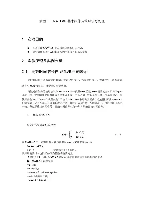
1. 单位阶跃序列单位阶跃序列)(n u 定义为)0()0(01)(<≥⎩⎨⎧=n n n u (1-1)在MA TLAB 中,冲激序列可以通过编写uDT .m 文件来实现,即function y=uDT(n)y=n>=0; %当参数为非负时输出1调用该函数时n 也同样必须为整数或整数向量。
【实例1-1】 利用MATLAB 的uDT 函数绘出单位阶跃序列的波形图。
解:MATLAB 源程序为>>n=-3:5; >>x=uDT(n);>>stem(n,x,'fill'),xlabel('n'),grid on >>title('单位阶跃序列') >>axis([-3 5 -0.1 1.1])程序运行结果如图1-1所示。
2. 矩形序列矩形序列)(n R N 定义为),0()10(01)(N n n N n n R N ≥<-≤≤⎩⎨⎧= (1-2)矩形序列有一个重要的参数,就是序列宽度N 。
南昌航空大学实验报告2012 年 04 月 06 日课程名称: 数字信号处理 实验名称: 离散信号及其MATLAB 实现 班级: 090423班 学号: 09042303 姓名: 张 丽实验一 离散信号及其MATLAB 实验一、实验目的(1)熟悉MATLAB 的主要操作命令;(2)学会离散信号的表示方法及其基本运算; (3)掌握简单的绘图命令;(4)用Matlab 编程并学会创建函数。
二、实验内容(1)序列的加、减、乘、除和乘方运算。
输入A=[1 2 3 4 ],B=[3 4 5 6],起点n=0,求C=A+B ,D=A-B ,E=A.*B ,F=A./B ,G=A.^B ,并用stem 语句画出A ,B ,C ,D ,E ,F ,G 。
(2)用MATLAB 实现下列序列:① x(n)=n 8.0 0≤n ≤15 ② x(n)=n j e )32.0( 0≤n ≤15③ x(n)=3cos(0.125πn+0.2π)+2sin(0.25πn+0.1π) 0≤n ≤15(3)编写函数如stepshift (n0,n1,n2)实现u(n)的移动序列u(n-n0),n1≤n ≤n2,给出该函数的图形。
设n1=0,n2=9,n0=2(4) x(n)=[1,-1,3,5],起点n=0,产生并绘出下列序列的样本: x1(n)=2x(n+2)-x(n-1)-2x(n)三、实验程序及实验图形 实验(1) 1、 程序:n=[0:3];A=[1 2 3 4 ]; %定义序列A ,即一行四列的矩阵 B=[3 4 5 6]; %定义序列BC=A+B;D=A-B;E=A.*B;F=A./B;G=A.^B; figure(1);subplot(2,2,1) %将图形界面分成2行2列,其中第一个显示下列图形 stem(n,A,'r*'); %绘制二维离散数据的火柴杆图,用红线和*号标出xlabel('n'); %x 轴标签为n ylabel('A'); %y 轴标签为A grid on; %绘制网格 subplot(2,2,2)stem(n,B);xlabel('n');ylabel('B');grid on; subplot(2,2,3)stem(n,C);xlabel('n');ylabel('C');grid on;title('序列的运算'); subplot(2,2,4);stem(n,D);xlabel('n');ylabel('D');grid on; figure(2);subplot(3,1,1)stem(n,E);xlabel('n');ylabel('E');grid on;title('序列的运算'); subplot(3,1,2)stem(n,F);xlabel('n');ylabel('F');grid on; subplot(3,1,3)stem(n,G);xlabel('n');ylabel('G');grid on;2、 运行结果nAnBnCnD图1 A 、B 、C 、D 的波形nE序列的运算nFnG图2 E 、F 、G 的波形3、 实验结果分析:由图1和图2可知:序列的加、减、乘、除是在n 上的对应点的加、减、乘、除,.*、./、.^也是矩阵的对应点相乘、除、乘方,对离散序列进行运算可以看作是对两个行向量的运算。
实验1 离散时间信号的时域分析一、实验目的(1)了解MATLAB 语言的主要特点及作用;(2)熟悉MATLAB 主界面,初步掌握MATLAB 命令窗和编辑窗的操作方法;(3)学习简单的数组赋值、数组运算、绘图的程序编写;(4)了解常用时域离散信号及其特点;(5)掌握MATLAB 产生常用时域离散信号的方法。
二、知识点提示本章节的主要知识点是利用MATLAB 产生数字信号处理的几种常用典型序列、数字序列的基本运算;重点是单位脉冲、单位阶跃、正(余)弦信号的产生;难点是MATLAB 关系运算符“==、>=”的使用。
三、实验内容1. 在MATLAB 中利用逻辑关系式0==n 来实现()0n n -δ序列,显示范围21n n n ≤≤。
(函数命名为impseq(n0,n1,n2))并利用该函数实现序列:()()()632-+-=n n n y δδ;103≤≤-nn 0212. 在MATLAB 中利用逻辑关系式0>=n 来实现()0n n u -序列,显示范围21n n n ≤≤。
(函数命名为stepseq(n0,n1,n2))并利用该函数实现序列:()()()20522≤≤--++=n n u n u n y3. 在MATLAB 中利用数组运算符“.^”来实现一个实指数序列。
如: ()()5003.0≤≤=n n x n4. 在MATLAB 中用函数sin 或cos 产生正余弦序列,如:()()2003.0cos 553.0sin 11≤≤+⎪⎭⎫ ⎝⎛+=n n n n x πππ5. 已知()n n x 102cos 3π=,试显示()()()3,3,+-n x n x n x 在200≤≤n 区间的波形。
6. 参加运算的两个序列维数不同,已知()()6421≤≤-+=n n u n x ,()()8542≤≤--=n n u n x ,求()()()n x n x n x 21+=。

MATLAB通信系统仿真实验报告实验一、MATLAB的基本使用与数学运算目的:学习MATLAB的基本操作,实现简单的数学运算程序。
内容:1-1 要求在闭区间[0,2π]上产生具有10个等间距采样点的一维数组。
试用两种不同的指令实现。
运行代码:x=[0:2*pi/9:2*pi]运行结果:1-2 用M文件建立大矩阵xx=[ 0.1 0.2 0.3 0.4 0.5 0.6 0.7 0.8 0.91.1 1.2 1.3 1.4 1.5 1.6 1.7 1.8 1.92.1 2.2 2.3 2.4 2.5 2.6 2.7 2.8 2.93.1 3.2 3.3 3.4 3.5 3.6 3.7 3.8 3.9]代码:x=[ 0.1 0.2 0.3 0.4 0.5 0.6 0.7 0.8 0.91.1 1.2 1.3 1.4 1.5 1.6 1.7 1.8 1.92.1 2.2 2.3 2.4 2.5 2.6 2.7 2.8 2.93.1 3.2 3.3 3.4 3.5 3.6 3.7 3.8 3.9]m_mat运行结果:1-3已知A=[5,6;7,8],B=[9,10;11,12],试用MATLAB分别计算A+B,A*B,A.*B,A^3,A.^3,A/B,A\B.代码:A=[5 6;7 8] B=[9 10;11 12] x1=A+B X2=A-B X3=A*B X4=A.*B X5=A^3 X6=A.^3 X7=A/B X8=A\B运行结果:1-4任意建立矩阵A,然后找出在[10,20]区间的元素位置。
程序代码及运行结果:代码:A=[12 52 22 14 17;11 10 24 03 0;55 23 15 86 5 ] c=A>=10&A<=20运行结果:1-5 总结:实验过程中,因为对软件太过生疏遇到了些许困难,不过最后通过查书与同学交流都解决了。
例如第二题中,将文件保存在了D盘,而导致频频出错,最后发现必须保存在MATLAB文件之下才可以。
MatLab 仿真试验 ---------“数字信号处理”课实验一:数字信号的 FFT 分析1、实验内容及要求(1) 离散信号的频谱分析: 设信号此信号的0.3pi 和 0.302pi 两根谱线相距很近,谱线 0.45pi 的幅度很小,请选择合适的序列长度 N 和窗函数,用 DFT 分析其频谱,要求得到清楚的三根谱线。
(2) DTMF 信号频谱分析用计算机声卡采用一段通信系统中电话双音多频(DTMF )拨号数字 0~9的数据,采用快速傅立叶变换(FFT )分析这10个号码DTMF 拨号时的频谱。
2、实验目的通过本次实验,应该掌握:(a) 用傅立叶变换进行信号分析时基本参数的选择。
(b) 经过离散时间傅立叶变换(DTFT )和有限长度离散傅立叶变换(DFT ) 后信号频谱上的区别,前者 DTFT 时间域是离散信号,频率域还是连续的,而 DFT 在两个域中都是离散的。
(c) 离散傅立叶变换的基本原理、特性,以及经典的快速算法(基2时间抽选法),体会快速算法的效率。
(d) 获得一个高密度频谱和高分辨率频谱的概念和方法,建立频率分辨率和时间分辨率的概念,为将来进一步进行时频分析(例如小波)的学习和研究打下基础。
(e) 建立 DFT 从整体上可看成是由窄带相邻滤波器组成的滤波器组的概念,此概念的一个典型应用是数字音频压缩中的分析滤波器,例如 DVD AC3 和MPEG Audio 。
实验二: DTMF 信号的编码1、实验内容及要求1)把您的联系电话号码 通过DTMF 编码生成为一个 .wav 文件。
技术指标:根据 ITU Q.23 建议,DTMF 信号的技术指标是:传送/接收率为每秒 10 个号码,或每个号码 100ms 。
每个号码传送过程中,信号存在时间至少 45ms ,且不多于 55ms ,100ms 的其余时间是静音。
在每个频率点上允许有不超过 ±1.5% 的频率误差。
任何超过给定频率 ±3.5% 的信号,均被认为是无效的,拒绝接收。

《信号与系统》MATLAB仿真实验讲义(第二版)肖尚辉编写宜宾学院电信系电子信息教研室《信号与系统》课程2004年3月 宜宾使用对象:电子专业02级3/4班(本科)实验一 产生信号波形的仿真实验一、实验目的:熟悉MATLAB软件的使用,并学会信号的表示和以及用MATLAB来产生信号并实现信号的可视化。
二、实验时数:3学时+3学时(即两次实验内容)三、实验内容:信号按照自变量的取值是否连续可分为连续时间信号和离散时间信号。
对信号进行时域分析,首先需要将信号随时间变化的规律用二维曲线表示出来。
对于简单信号可以通过手工绘制其波形,但对于复杂的信号,手工绘制信号波形显得十分困难,且难以绘制精确的曲线。
在MATLAB中通常用三种方法来产生并表示信号,即(1)用MATLAB软件的funtool符合计算方法(图示化函数计算器)来产生并表示信号;(2)用MATLAB软件的信号处理工具箱(Signal Processing Toolbox)来产生并表示信号;(3)用MATLAB软件的仿真工具箱Simulink中的信号源模块。
(一) 用MATLAB软件的funtool符合计算方法(图示化函数计算器)来产生并表示信号在MATLAB环境下输入指令funtool,则回产生三个视窗。
即figure No.1:可轮流激活,显示figure No.3的计算结果。
figure No.2:可轮流激活,显示figure No.3的计算结果。
figure No.3:函数运算器,其功能有:f,g可输入函数表达式;x是自变量,在缺省时在[-2pi,2pi]的范围内;自由参数是a;在分别输入完毕后,按下面四排的任一运算操作键,则可在figure No.1或figure No.2产生相应的波形。
学生实验内容:产生以下信号波形3sin(x)、5exp(-x)、sin(x)/x、1-2abs(x)/a、sqrt(a*x)(二) 用MATLAB软件的信号处理工具箱(Signal Processing Toolbox)来产生并表示信号一种是用向量来表示信号,另一种则是用符合运算的方法来表示信号。
MATLAB实验讲义目录实验大纲 (2)实验一/二 MATLAB的基础操作 (3)实验三 MATLAB运算基础(一) (3)实验四 MATLAB运算基础(二) (4)实验五循环结构程序设计(一) (5)实验六循环结构程序设计(二) (5)实验七 MATLAB的绘图操作(一) (6)实验八 MATLAB的绘图操作(二) (7)实验九函数和文件(一) (7)实验十函数和文件(二) (7)实验十一线性代数中的数值计算问题 (8)实验十二 MATLAB函数库的运用(一) (9)实验十三 MATLAB函数库的运用(二) (10)《MATLAB》课程实验教学大纲课程名称:MATLAB(MATLAB)课程编号:16072327课程性质:选修实验总学时:27实验室名称:电子设计自动化一、课程简介:本课程是电气工程及其自动化、自动化、电力工程与管理专业本科生的学科基础选修课,它在线性代数、信号分析和处理、控制系统设计和仿真等方面有着广泛的应用。
主要是学习MATLAB的语法规则、基本命令和使用环境,使学生掌握MATLAB的基本命令和基本程序设计方法,提高使用该语言的应用能力,具有使用MATLAB语言编程和调试的能力,以便为后续多门课程使用该语言奠定必要的基础。
二、课程实验目的与要求:1.基本掌握MATLAB在线帮助功能的使用、熟悉MATLAB运行环境和MATLAB语言的主要特点,掌握MATLAB语言的基本语法规则及基本操作命令的使用,学会M文件的建立和使用方法以及应用MATLAB实现二维和三维图形的绘制方法,具有使用MATLAB语言编程和调试的能力。
2.初步掌握MATLAB在电路和信号与系统中的应用。
3.能根据需要选学参考书,查阅手册,通过独立思考,深入钻研有关问题,学会自己独立分析问题、解决问题,具有一定的创新能力。
三、主要仪器设备及台(套)数:计算机50台、MATLAB软件五、主要参考书目:1.《MATLAB及在电子信息课程中的应用》陈怀琛、杨吉斌编著,电子工业出版社,2002年1版2.《MATLAB7.0编程基础》王家文、王皓、刘海等;机械工业出版社,2005年7月3.《MATLAB教程——基于6.x版本》张志涌、徐彦琴等;北京航空航天大学出版,2001年4月出版实验一/二 MATLAB的基础操作一、实验目的1、掌握MATLAB的启动和退出。
MATLAB的综合实验一、实验目的及要求培养学生利用Matlab解决专业问题的能力。
二、实验设备(环境)及要求1.计算机2.Matlab软件编程实验平台三、实验内容1、编程实现一个数字信号处理的仿真系统。
要求具有界面并实现以下功能:1)能产生(得到)并选择各种数字信号(sin、方波、三角波、语音、噪声及其叠加);2)具有DFT、DCT和DWT变换功能,并对各种信号进行变换;3)设计滤波器实现低通、高通、带通滤波,得到输出信号的频域特性和时间序列;4)输入一段叠加了噪声的语音信号,显示其频谱特性,通过变换或滤波对其降噪,得到输出信号的频域特性和时间序列。
四、设计思想本系统包含有三个主要部分:信号产生与变换模块,滤波器模块和语音噪声处理。
信号产生与变换通过输入信号频率和采样频率实现正弦、方波、三角波、语音信号的产生以及噪声的叠加,系统设定信号持续时间为0.05s,语音信号为截取了一段2s的声音信号。
同时对各个信号进行DFT,DCT和DWT变换,且变换点数N=256,同时设定DWT变换时的小波类型为db1。
滤波器模块设计了四个IIR 滤波器(巴特沃斯、切比雪夫Ⅰ型,切比雪夫Ⅱ型和椭圆滤波器),并分别实现低通,高通和带通。
界面设计了各种滤波器所需参数的输入模块。
系统设定待滤波信号持续时间为0.05s,包含有3个频率成分,S=sin(2*pi*f*t)+ sin(2*pi*5*f*t)+sin(2*pi*8*f*t),其中f为输入信号频率,S通过低通、带通、高通滤波器之后,分别得到频率为f,5f和8f的正弦信号,实现信号滤波。
语音噪声处理部分是一个复选框按钮,通过巴特沃斯低通滤波器对其进行降噪,设计中通过观察噪声语音信号的频谱得到低通滤波器的截止频率和阻带起始频率,并合理输入通带衰减与阻带衰减,最终得到理想的降噪结果。
数字滤波器设计过程中用到了如下的一些matlab设计函数:buttord、butter,cheb1ord、cheby1,cheb2ord、cheby2,ellipord、ellip。
实验⼀MATLAB编程环境及常⽤信号的⽣成及波形仿真实验⼀ MATLAB 编程环境及常⽤信号的⽣成及波形仿真⼀、实验⽬的1、学会运⽤Matlab 表⽰常⽤连续时间信号的⽅法2、观察并熟悉这些信号的波形和特性:3、实验内容:编程实现如下常⽤离散信号:单位脉冲序列,单位阶跃序列,矩形序列,实指数序列,正弦序列,复指数序列;⼆、实验原理及实例分析2、如何表⽰连续信号?从严格意义上讲,Matlab 数值计算的⽅法不能处理连续时间信号。
然⽽,可利⽤连续信号在等时间间隔点的取样值来近似表⽰连续信号,即当取样时间间隔⾜够⼩时,这些离散样值能被Matlab 处理,并且能较好地近似表⽰连续信号。
3、Matlab 提供了⼤量⽣成基本信号的函数。
如:(1)指数信号:K*exp(a*t)(2)正弦信号:K*sin(w*t+phi)和K*cos(w*t+phi)(3)复指数信号:K*exp((a+i*b)*t)(4)抽样信号:sin(t*pi)注意:在Matlab 中⽤与Sa(t)类似的sinc(t)函数表⽰,定义为:)t /()t (sin )t (sinc ππ=(5)矩形脉冲信号:rectpuls(t,width)(6)周期矩形脉冲信号:square(t,DUTY),其中DUTY 参数表⽰信号的占空⽐DUTY%,即在⼀个周期脉冲宽度(正值部分)与脉冲周期的⽐值。
占空⽐默认为0.5。
(7)三⾓波脉冲信号:tripuls(t, width, skew),其中skew 取值范围在-1~+1之间。
(8)周期三⾓波信号:sawtooth(t, width)(9)单位阶跃信号:y=(t>=0)常⽤的图形控制函数1)学习clc, dir(ls), help, clear, format,hold, clf控制命令的使⽤和M⽂件编辑/调试器使⽤操作;2)主函数函数的创建和⼦程序的调⽤;3)plot,subplot, grid on, figure, xlabel,ylabel,title,hold,title,Legend,绘图函数使⽤;axis([xmin,xmax,ymin,ymax]):图型显⽰区域控制函数,其中xmin为横轴的显⽰起点,xmax为横轴的显⽰终点,ymin为纵轴的显⽰起点,ymax为纵轴的显⽰终点。
信号处理仿真(MATLAB)实验指导书青岛大学自动化工程学院电子工程系2011年4月MATLAB 实验一一、实验目的:1. Be familiar with MATLAB Environment2. Be familiar with array and matrix二、实验内容:1. Be familiar with Matlab 6.5Startup Matlab 6.5, browse the major tools of the Matlab desktop⏹ The Command Windows⏹ The Command History Windows⏹ Launch Pad⏹ The Edit/Debug Window⏹ Figure Windows⏹ Workspace Browser and Array Editer⏹ Help Browser⏹ Current Directory BrowserPART I:下列选择练习,不需提交实验报告1. Give the answer of the following questions for the array1.10.02.13.560.01.16.62.83.412.10.10.30.41.31.45.10.01.10.0a r r a y -⎡⎤⎢⎥-⎢⎥=⎢⎥-⎢⎥-⎣⎦ 1)What is the size of array1?2)What is the value of array1(4,1)?3)What is the size and value of array1(:,1:2)?4) What is the size and value of array1([1 3], end)?2. Give the answer of the following commad1) a=1:2:5; 2) b=[a ’ a ’ a ’]; 3) c=b(1:2:3,1:2:3);4) d=a+b(2,:) 5) w=[zeros(1,3) ones(3,1)’ 3:5’]3. Give the answer of the sub-arrays1.10.02.13.560.01.16.62.83.412.10.10.30.41.31.45.10.01.10.0a r r a y -⎡⎤⎢⎥-⎢⎥=⎢⎥-⎢⎥-⎣⎦ 1) array1(3,:); 2) array1(:,3); 3) array1(1:2:3,[3 3 4]) 4) array1([1 1],:)4. Give the answer of the following operations22111,,,(2)12022a b c d e y e --⎡⎤⎡⎤⎡⎤====⎢⎥⎢⎥⎢⎥--⎣⎦⎣⎦⎣⎦ 1) a+b 2) a*d 3) a.*d 4) a*c5) a.*c 6)a\b 7) a.\b 8)a.^bEXERCISE II:TEXT BOOK (4TH EDITION) PAGE 17-18:1.1, 1.4, 1.7MATLAB实验二一、实验目的:1. Be familiar with array and matrix2. Be familiar with MATLAB operations and simple plot functionPART I:下列选择练习,不需提交实验报告1.Edit & Run the m-file% test step response functionwn=6; kosi=[0.1:0.1:1.0 2];figure(1); hold onfor kos=kosinum=wn^2; den=[1,2*kos*wn,wn.^2]; step(num,den)endhold off;2.Edit & Run the m-file% test plot functionx=0:pi/20:3*pi; y1=sin(x); y2=2*cos(2*x); plot(x,y1,'rv:',x,y2,'bo--');title('Plot the Line of y=sin(2x) and its derivative'); xlabel('X axis'); ylabel('Y axis');legend('f(x)','d/dx f(x)'); grid on;3.Edit & Run the m-file% test subplot and loglog functionx=0:0.1:10; y=x.^2-10.*x+26;subplot(2,2,1); plot(x,y); grid on;subplot(2,2,2); semilogx(x,y); grid on;subplot(2,2,3); semilogy(x,y); grid on;subplot(2,2,4); loglog(x,y); grid on;4.Edit & Run the m-file% test max and plot functionvolts=120; rs=50; rl=1:0.1:100;amps=volts./(rs+rl); pl=(amps.^2).*rl; [maxvol,index]=max(pl);plot(rl,pl,rl(index),pl(index),'rh'); grid on;PART II:下列选择练习,需提交实验报告EXERCISE II:TEXT BOOK (4TH EDITION) PAGE 69-73:2.9 , 2.11, 2.13, 2.14,2.17 , 2.18MATLAB 实验三一、实验目的:1. Learn to design branch statements program2. Be familiar with relational and logical operators3. Practice 2D plotting二、实验内容:PART I: (选择练习,不需提交实验报告)1. Hold command exercisex=-pi:pi/20:pi;y1=sin(x); y2=cos(x); plot(x,y1, 'b-'); hold on;plot(x,y2, 'k--'); hold off;legend ('sinx', 'cosx')2. Figure command exercisefigure(1);subplot(2,1,1);x=-pi:pi/20:pi; y=sin(x); plot(x,y); grid on;title('Subplot 1 Title');subplot(2,1,2);x=-pi:pi/20:pi; y=cos(x); plot(x,y); grid on;title('Subplot 2 Title');3. Polar Plots exerciseg=0.5;theta=0:pi/20:2*pi;gain=2*g*(1+cos(theta));polar(theta,gain,'r-');title('\fontsize{20} \bfGain versus angle \theta');4. Assume that a,b,c, and d are defined, and evaluate the following expression.a=20; b=-2; c=0; d=1;(1) a>b; (2) b>d; (3) a>b&c>d; (4) a==b; (5) a&b>c; 6) ~~b;a=2; b=[1 –2;-0 10]; c=[0 1;2 0]; d=[-2 1 2;0 1 0];(7) ~(a>b) (8) a>c&b>c (9) c<=da=2; b=3; c=10; d=0;(10) a*b^2>a*c (11) d|b>a (12) (d|b)>aa=20; b=-2; c=0; d=’Test’;(13) isinf(a/b) (14) isinf(a/c) (15) a>b&ischar(d) (16) isempty(c)5. Write a Matlab program to solve the function 1()ln1y x x =-, where x is a number <1.Use an if structure to verify that the value passed to the program is legal. If the value of x is legal, caculate y(x). If not ,write a suitable error message and quit.PART II: (需提交实验报告)1. Write out m. file and plot the figures with gridsAssume that the complex function f(t) is defined by the equationf(t)=(0.5-0.25i)t-1.0Plot the amplitude and phase of function for 0 4.t ≤≤2. Write the Matlab statements required to calculate y(t) from the equation22350()350t t y t t t -+≥⎧=⎨+<⎩for value of t between –9 and 9 in steps of 0.5. Use loops and branches to perform this calculation.EXERCISE II:TEXT BOOK (4TH EDITION) PAGE 121-124:3.1, 3.3 , 3.5, 3.6, 3.7, 3.11, 3.14一、实验目的:1. Learn to design loop statements program2. Be familiar with relational and logical operators3. Practice 2D plotting二、实验内容:PART I: (选择练习,不需提交实验报告)pare the 3 approaches follows (Loops and Vectorization)%A. Perform calculation by For Loop with pre-initialize arraytic;square=zeros(1,10000) %pre-initialize arrayfor ii=1:10000square(ii)=ii^2;square_root(ii)=ii^(1/2);cube_root(ii)=ii^(1/3);endtoc; t1=toc%B. Perform calculation by For Loop without pre-initialize arraytic;for ii=1:10000square(ii)=ii^2;square_root(ii)=ii^(1/2);cube_root(ii)=ii^(1/3);endtoc; t2=toc%C. Perform calculation with vectorstic;ii=1:10000square(ii)=ii.^2;square_root(ii)=ii.^(1/2);cube_root(ii)=ii.^(1/3);endtoc; t3=tocEXERCISE II:TEXT BOOK (4TH EDITION) PAGE 165-171: 4.7,4.16,4.18,4.19,4.20,4.27一、实验目的:1. Learn to write MATLAB functions2. Be familiar with complex data and character data3. Practice 2D plotting二、实验内容:1. Write three Matlab functions to calculate the hyperbolic sine, cosine, and tangent functions:s i n h (),c o s h (),t a n ()22x xx x x x x x e e e e e e h e e -----+-=+ then plot the shapes of hyperbolic sine, cosine, and tangent functions on one figure, 55x -≤≤.2. Write a program use the function 32()552f x x x x =-+- and plot the line, and search for the minimum and maximum in 200 steps over the range of 13x -≤≤, mark the minimum and maximum on the line figure.3. Write a function to calculate the distance between two points 11(,)x y and 22(,)x y , that the points should be given by ‘input ’ function.4. Write a function complex_to that accept a complex number var , and returns two output arguments containing the magnitude mag and angle theta of the complex number. The output angle should be in degrees.Write another function polar_to_complex that accepts two input arguments containing the magnitude mag and angle theta of the complex number in degrees, and returns the complex number var .4. Write a program that accepts a series of strings from a user with the input function, sorts the strings into ascending order, and prints them out.EXERCISE II:TEXT BOOK (4TH EDITION) PAGE 213-223: 5.10, 5.11, 5.19, 5.25, 5.26, 5.33一、实验目的:1. Learn to write MATLAB functions2. Be familiar with complex data and character data5. Practice 2D plotting二、实验内容:1. Write three Matlab functions to calculate the hyperbolic sine, cosine, andtangent functions:s i n h (),c o s h (),t a n ()22x xx x x x x x e e e e e e h e e -----+-=+ then plot the shapes of hyperbolic sine, cosine, and tangent functions on one figure, 55x -≤≤.2. Write a program use the function 32()552f x x x x =-+- and plot the line,and search for the minimum and maximum in 200 steps over the range of 13x -≤≤, mark the minimum and maximum on the line figure.3. Write a function to calculate the distance between two points 11(,)x y and 22(,)x y , that the pointsshould be given by ‘input ’ function.4. Write a function complex_to that accept a complex number var , and returns two output arguments containing the magnitude mag and angle theta of the complex number. The output angle should be in degrees.Write another function polar_to_complex that accepts two input arguments containing the magnitude mag and angle theta of the complex number in degrees, and returns the complex number var .5. Write a program that accepts a series of strings from a user with the input function, sorts the strings into ascending order, and prints them out.EXERCISE II:TEXT BOOK (4TH EDITION) PAGE 265-267:6.2, 6.10, 6.11一、实验目的:1. Practice 2D plotting and 3D plotting2. Learn to use fplot function3. Be familiar with cell arrays and structure arrays二、实验内容:1. Give the 3D plot figure of 0.30.1()sin(3),()cos()t t x t e t y t e t --== use plot3 function, 020x ≤≤, and grid on, linewidth is 3.0.2. Plot the function sin x y e x -=, 02x ≤≤, step 0.1. Create the following plot types: (a) stem plot; (b) stair plot; (c) bar plot; (d) compass plot.3. Plot the function ()f x = over the range 0.110.0x ≤≤ using function fplot, and grid on.4. Create a cell arrays:5. Create a structure arrays and to calculate the mean billing of three patients:一、实验目的:Be familiar with Input/Output functions二、实验内容:1. Write a m-file. The m-file creates an array containing 150⨯random values, sorts the array into ascending order, opens a user-specified file for writing only, then writes the array to disk in 32-bit floating-point format , and close the file. It then opens the file and read the data back into 510⨯array.2. Edit a file as data4_4.txt that contains 44⨯square matrix, then import the array use uiimport function, and calculate the inverse of the square matrix .3.Write a program to read a set of integers from an input data file, and locate the largest andsmallest values within the data file. Print out the largest and smallest values, together with the lines on which they were found in one figure.一、实验目的:1.Be familiar with sound file2. Learn about create sound and use speaker.3. Making Music with MATLAB二、实验内容:Before we actually start making music, let's revise a few AC waveform basics. Consider the sine wave shown in the figure below:The sine wave shown here can be described mathematically as:v = A sin 2 π f twhere A is the Amplitude (varying units), f is the frequency (Hertz) and t is the time (seconds).T is known as the time period (seconds) and T=1/fBased on the equation,when t=0; v = A sin 2 π f(0) = 0when t=T/4; v = A sin 2 π f (T/4) = A sin 2 π f(1/4f) = A sin ( π/2) = A;when t=T/2; v = A sin 2 π f (T/2) = A sin 2 π f(1/2f) = A sin ( π) = 0;and so on.Sound waves are created when a waveform as shown here is used to vibrate molecules in a material mediumat audio frequencies (300 Hz <= f <= 3 kHz).If you wish to create a waveform such as the one shown in the figure, you would need to evaluate the function, v = A sin 2 π f t, at discrete times, t (shown as the time instants of the red dots), typically at equal time intervals. These time intervals must be "sufficiently" small (how small is small? Remember the Nyquist criterion?..........) to obtain a "smooth" waveform.This time interval is called the "Sampling Interval" and the process of breaking up a continuous waveform by specifying it only at discrete points in time is called sampling. (you should already know much of this stuff from the previous Clinic on Data Acquisition Basics).The sampling interval, shown here is T s; corresponding to that there exists a "Sampling Frequency", fs = 1/T s.As an example, the MATLAB code to create a sine wave of amplitude A = 1, at audio frequency of 466.16Hz (corresponds to A# in the Equal Tempered Chromatic Scale) would be:>> v = sin(2*pi*466.16*[0:0.000125:1.0]);The vector, v, now contains samples of the sine wave, starting at t=0 s, to t=1.0 s, in samples spaced 0.000125 s apart (the sampling interval T s). This corresponds to a sampling frequency of 8 KHz, which is standard for voice grade audio channel.Now, you can either plot this sine wave; or you can hear it!!!To plot, simply do>> plot(v);To hear v, you need to convert the data contained in v to some standard audio format that can be played using a Sound Card and Speakers on your PC. One such standard audio format is called the "wav" format. Matlab provides a function called wavwrite to convert a vector into wav format and save it on disk. Do >> help wavwrite for more details. Now, to create a wav file, do>> wavwrite(v, 'asharp.wav'); (you can give any file name between the ' ' s)Now, you can "play" this wav file called asharp.wav using any multimedia player. For example, you could use the Sound Recorder program. Start this by pointing to Start - Programs - Accessories - Multimedia - Sound Recorder. Open the wav file using the File Menu and press Play. If you have installed a sound card and a pair of speakers on your PC, you should be able to hear a short note.Now that you can make a single note, you can put notes together and make music!!!Let's look at the following piece of music:A A E E F# F# E ED D C#C# B B A AE E D D C# C# B B (repeat once)(repeat first two lines once)The American Standard Pitch for each of this notes is:A: 440.00 HzB: 493.88 HzC#: 554.37 HzD: 587.33 HzE: 659.26 HzF#: 739.99 HzAssuming each note lasts for 0.5 seconds, the MA TLAB m-file for creating a wav file for this piece of music would be:clear;a=sin(2*pi*440*(0:0.000125:0.5));b=sin(2*pi*493.88*(0:0.000125:0.5));cs=sin(2*pi*554.37*(0:0.000125:0.5));d=sin(2*pi*587.33*(0:0.000125:0.5));e=sin(2*pi*659.26*(0:0.000125:0.5));fs=sin(2*pi*739.99*(0:0.000125:0.5));line1=[a,a,e,e,fs,fs,e,e,];line2=[d,d,cs,cs,b,b,a,a,];line3=[e,e,d,d,cs,cs,b,b];song=[line1,line2,line3,line3,line1,line2];wavwrite(song,'song.wav');HINT: Before you code the entire song, just code the first line, create a wav file, play it and make sure everything works.MATLAB实验十-十六。