A general framework for types in graph rewriting

*
instances will be regarded as the same class
and be connected with the same weight,
which in turn pulls these missing instances
together in the low-dimensional subspace
●*
T
H
A
N
K
Y
O
U
The proposed method significantly outperforms the other methods on the above multi-view databases with all kinds of incomplete cases. For instance, on the handwritten digit database (Table II), the proposed method achieves 3% and 6% improvement of ACC and NMI in comparison with the second best method. 【Clarifying experimental results and analyze the results by giving an example. 】
Example two
*
Complexity
Academic writing is gramatically more complex than other forms of writing.
Inspired by this motivation, Gao et al. [30]
*

高二英语软件开发单选题50题1.The main language used in software development is _____.A.PythonB.JavaC.C++D.All of the above答案：D。

在软件开发中，Python、Java 和C++都是常用的编程语言，所以答案是以上皆是。

2.Which one is not a software development tool?A.Visual StudioB.IntelliJ IDEAC.PhotoshopD.Eclipse答案：C。

Photoshop 是图像编辑软件，不是软件开发工具。

Visual Studio、IntelliJ IDEA 和Eclipse 都是常用的软件开发集成环境。

3.The process of finding and fixing bugs in software is called _____.A.debuggingB.codingC.testingD.designing答案：A。

debugging 是调试的意思，即查找和修复软件中的错误。

coding 是编码，testing 是测试，designing 是设计。

4.A set of instructions that a computer follows is called a _____.A.programB.algorithmC.data structureD.variable答案：A。

program 是程序，即一组计算机遵循的指令。

algorithm 是算法，data structure 是数据结构，variable 是变量。

5.Which programming paradigm emphasizes on objects and classes?A.Procedural programmingB.Functional programmingC.Object-oriented programmingD.Logic programming答案：C。

Abstract
Introduction
methodology
results
Discussion/conclusion
The contents of a research article or thesis
*
融资项目商业计划书
单击此处添加副标题
*
Warming up question:
what kind of research methods do you use in your field.?
APA format
*
融资项目商业计划书
单击此处添加副标题
General structure of the methods Section
*
融资项目商业计划书
单击此处添加副标题
*
融资项目商业计划书
单击此处添加副标题
*
融资项目商业计划书
单击此处添加副标题
*
融资项目商业计划书
单击此处添加副标题
*
融资项目商业计划书
单击此处添加副标题
definition
*
Quantitative the systematic empirical investigation of observable phenomena via statistical, mathematical or computational techniques.
3
Model analysis-Sentence1
*
practice: read the 3 examples and decide what are the ways to introduce the Methodology? ways

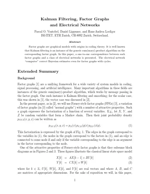
Kalman Filtering,Factor Graphsand Electrical NetworksPascal O.Vontobel,Daniel Lippuner,and Hans-Andrea LoeligerISI-ITET,ETH Zurich,CH-8092Zurich,Switzerland.AbstractFactor graphs are graphical models with origins in coding theory.It is well known that Kalmanfiltering is an instance of the generic sum(mary)-product algorithm on thecorresponding factor graph.In this paper,a one-to-one correspondence between suchfactor graphs and a class of electrical networks is presented.The electrical network“computes”correct Bayesian estimates even for factor graphs with cycles. Extended SummaryBackgroundFactor graphs[1]are a unifying framework for a wide variety of system models in coding, signal processing,and artificial intelligence.Many important algorithms in thesefields are instances of the generic sum(mary)-product algorithm,which works by message passing in the factor graph.One such instance is Kalmanfiltering and smoothing;for the scalar case, this was shown in[1],the vector case was discussed in[2].In the present paper,as in[2],we will use Forney-style factor graphs(FFGs)[3],a variation of factor graphs(in[3]called“normal graphs”)with a number of attractive properties.Such a graph expresses the factorization of a function of several variables. E.g.,let X,Y,and Z be random variables that form a Markov chain.Then their joint probability density p XY Z(x,y,z)can be written asp XY Z(x,y,z)=p X(x)p Y|X(y|x)p Z|Y(z|y).(1)This factorization is expressed by the graph of Fig.1.The edges in the graph correspond to the variables in(1),the nodes in the graph correspond to the factors in(1),and an edge is connected to some node if and only if the variable corresponding to the edge is an argument in the factor corresponding to the node.One of the attractive properties of Forney-style factor graphs is that they subsume block diagrams as in Figures2and3.Thesefigures illustrate the classical linear state space modelX[k]=AX[k−1]+BU[k](2)Y[k]=CX[k]+W[k](3)where for k∈Z,U[k],W[k],X[k],and Y[k]are real vectors and where A,B,and C are matrices of appropriate dimensions.For the sake of exposition we will,in this paper,focus on the case where all these variables and matrices are scalars.The nodes in Figures 2and3are then defined to represent factors as shown in Table1(left column).In Kalman filtering,both U[.]and W[.]are usually assumed to be white Gaussian(“noise”)processes; the corresponding nodes in thesefigures are then of the type shown in the top row of Table1. The overall function(the factorization of)which is expressed by Figures2and3is the joint probability density of all involved variables.If the variables Y[k]are observed,say Y[k]=y k,the corresponding branches are“ter-minated”by nodes corresponding to factorsδ(y[k]−y k)(the dashed boxes in Fig.2);such factors may be viewed as degenerate cases of Gaussian distributions(top row of Table1) with variance zero.The graph then represents(the factorization of)the joint a posteriori density of all involved variables.As described in[1]and[2],Kalmanfiltering may be viewed as passing messages along the edges of these graphs;in general,the messages consist of mean vectors and covariance matrices(or inverses of covariance matrices)and are computed according to the rules of the generic sum-product algorithm.In its most narrow sense,Kalmanfiltering is only the forward sum-product recursion through the graph of Fig.2and yields the a posteriori probability distribution of the state X[k]given the observation sequence Y[.]up to time k.By computing also the backwards messages,the a posteriori probability of all quantities given the whole observation sequence Y[.]may be obtained.More generally,Kalmanfiltering amounts to the sum-product algorithm on any FFG(or part of an FFG)that consists of(the vector/matrix versions of)the linear building blocks listed in Table1(left column).As pointed out in[2],Kalmanfiltering in this sense is equivalent to a general least-squares algorithm.New ResultsInterestingly,the results of Kalmanfiltering(in its widest sense as defined above)can also be obtained by translating the state space model into an electrical network according to the rules of Table1.These networks consist of resistors,voltage sources,and transformers. (The latter are defined by the equations U2=aU1and I2=I1/a,where U i and I i are the voltage accross,and the current into,terminal pair i,i=1,2.)As shown in Table1,each edge/variable of the factor graph corresponds to a pair of nodes in the electrical network.Theorem.The voltages between such node pairs are the Bayesian estimates(i.e.,the means of the a posteriori marginal distributions)of the corresponding random variables.The equivalence of(traditional)Kalmanfiltering with an electrical network as in Table1 was recognized already by Carter[4].However,the above theorem holds also if the factor graph has cycles,which goes beyond[4](and appears to be related to the convergence results of[6]and[7]).In the electrical network,message passing according to the sum-product algorithm(and thus classical Kalmanfiltering)can be interpreted as follows.Each message represents aGaussian distribution as in the top row of Table1,and can thus be represented by a voltage source(corresponding to the mean)in series with a resistor(corresponding to the variance). As illustrated in Table2,the computation of messages out of the other node types in Table1 then amounts to connecting the incoming messages/circuits to the node circuit and reducing the resulting circuit to its Th´e venin equivalent circuit(i.e.,a voltage source in series with a resistor).We conclude with the following remarks:•The correspondence given in Table1can be extended to the vector case.•There is a dual version of the correspondence of Table1where the voltages and the currents are interchanged,as are series and parallel connections of subcircuits.•The representation of Kalmanfiltering(and smoothing)as an electrical network al-lows an easy transition from discrete-time Kalmanfiltering to continuous-time Kalman filtering.•A generalization beyond Kalmanfiltering/least squares was recently discovered by thefirst author[8]:if p(x,y,...)is any joint probability density function such that −log p(x,y,...)is convex,then a factor graph of p can be translated into an electrical network thatfinds the global maximum of p.The network consists of voltage sources (or current sources)and nonlinear resistors.Circuit simplifications similar to those in Table2correspond to the message passing rules of the max-product version(rather than the sum-product version)of generic sum(mary)-product algorithm.Moreover,if the voltages are solutions to the primal maximization problem,then the currents are the solutions to the dual problem.AcknowledgementThe authors thank S.Mitter for pointing out the book by Dennis[5],which inspired this work.p X Xp Y |X Y p Z |Y ZFigure 1:Forney-style factor graph (FFG)of a Markov chain....-X [k −1]?U [k ]?Z [k ]?Y [k ]-X [k ]?U [k +1]?Z [k +1]?Y [k +1]-X [k +1]...Figure 2:State space model.-X [k −1]A -?U [k ]B?+-=?C ?Z [k ]-X [k ]-W [k ]?Z [k ]+?Y [k ]Figure 3:Details of linear state space model.γe−(x −m )22σ2Xm ?m σ2?X 1δ(x −y )δ(x −z )=XZ Y r r?X ?Z -Y 2δ(x +y −z )+-X -Z 6Y?X ?Z -Y 3δ(y −ax )a-X -Y ¤¥¤¥¤¥§¦§¦§¦1:a ?X?Y Table 1:Correspondence between the nodes in the factor graph (left)and the components of the electrical network (right).All variables are scalars.1=X-Z -Y 6m Z =m X /σ2X +m Y /σ2Y 1/σ2X +1/σ2Y σ2Z =11/σ2X +1/σ2Y j σ2X m X j σ2Y m Y r r ⇒j σ2Z m Z2+-X --Z -6Y 6m Z =m X +m Y σ2Z =σ2X +σ2Y j σ2X m X j m Y σ2Y ⇒j σ2Z m Z3a -X --Y -m Y =am Xσ2Y =a 2σ2X j σ2X m X ¤¥¤¥¤¥§¦§¦§¦1:a⇒j σ2Y m YTable 2:Computation of messages (left and middle)with circuit interpretation (right).References[1] F.R.Kschischang,B.J.Frey,and H.-A.Loeliger,“Factor graphs and the sum-product algo-rithm,”IEEE rm.Theory,vol.IT–47,no.2,pp.498–519,2001.[2]H.-A.Loeliger,“Least squares and Kalmanfiltering on Forney graphs,”to appear in Codes,Graphs,and Systems,festschrift in honour of G.D.Forney,Kluwer,2001.[3]G.D.Forney,Jr.,“Codes on graphs:normal realizations,”IEEE rm.Theory,vol.IT-47,pp.520–548,Feb.2001.[4] D.W.Carter,“A circuit theory of the Kalmanfilter,”in Proc.32nd Conf.on Decision andControl(San Antonio,TX,USA),pp.1224–1226,Dec.1993.[5]J.B.Dennis,Mathematical Programming and Electrical Networks.MIT Press,Cambridge,Mass.,1959.[6]Y.Weiss and W.T.Freeman,“On the optimality of solutions of the max-product belief-propagation algorithm in arbitrary graphs,”IEEE rm.Theory,vol.47,pp.736–744, Feb.2001.[7]P.Rusmevichientong and B.Van Roy,“An analysis of belief propagation on the turbo decodinggraph with Gaussian densities,”IEEE rm.Theory,vol.47,pp.745–765,Feb.2001.[8]P.O.Vontobel,Kalman Filters,Factor Graphs,and Electrical Networks.Internal reportINT/200202,ISI-ITET,ETH Zurich,April2002.。

1. Introduction Network theory is an important tool for describing and analysing complex systems throughout the social, biological, physical, information and engineering sciences [1–3]. Originally, almost all studies of networks employed an abstraction in which systems are represented as ordinary graphs [4]: the ‘nodes’ (or ‘vertices’) of the graphs represent some entity or agent, and a tie between a pair of nodes is represented using a single, static, unweighted ‘edge’ (or ‘link’). Self- and multi-edges were also typically ignored. Although this approach is naive in many respects, it has been extremely successful. For example, it has been used to illustrate that many real networks possess a heavy-tailed degree distribution [5,6], exhibit the small-world property [7,8], contain nodes that play central roles [1,2] and/or have modular structures [9–11]. As research on complex systems has matured, it has become increasingly essential to move beyond simple graphs and investigate more complicated but more realistic frameworks. For example, edges often exhibit heterogeneous features: they can be directed [1,2,12], have different strengths (i.e. ‘weights’) [2,13,14], exist only between nodes that belong to different sets (e.g. bipartite networks) [1,2, 15] or be active only at certain times [16,17]. Most recently, there have been increasingly intense efforts to investigate networks with multiple types of connections (see Section 2.5) and so-called ‘network of networks’1 [19] (see Section 2.4). Such systems were examined decades ago in disciplines like sociology and engineering, but the explosive attempt to develop frameworks to study multilayer complex systems and to generalize a large body of familiar tools from network science is a recent phenomenon.2 In social networks, one can categorize edges based on the nature of the relationships (i.e. ties) or actions that they represent [2,21,22]. Reducing a social system to a network in which actors are connected in a pairwise fashion by only a single type of relationship is often an extremely crude approximation of reality. As a result, sociologists recognized decades ago that it is crucial to study social systems by constructing multiple social networks using different types of ties among the same set of individuals [2,23].3 For example, consider the sociograms4 that were drawn in the 1930s to represent social networks in a bank-wiring room [26]. These sociograms depicted relations between 14 individuals via 6 different types of social interactions (see Fig. 6(b)). In the sociology literature, networks in which each edge is categorized by its type are called ‘multiplex networks’ [27,28] or ‘multirelational networks’ [2]. (Such networks are also said to possess ‘multi-stranded’ relationships [29].) Social networks also often include several types of nodes (e.g. males and females) or hierarchical structures (e.g. individuals are part of organizations), which have been studied using ‘multilevel networks’ (see Section 2.8). The notion of a ‘network of networks’ also dates at least as far back as 1973 [30]. The tools

折线图英语作文Title: Exploring the Significance of Line Graphs。

Introduction:Line graphs are an indispensable tool in data representation, widely used across various fields such as economics, science, and social sciences. Their simplicity and effectiveness in illustrating trends and patterns make them a preferred choice for conveying information. In this essay, we delve into the importance and utility of line graphs.Importance of Line Graphs:Line graphs serve multiple purposes, primarily to visualize and analyze data trends over time or other continuous variables. They offer a clear depiction of how one variable changes in relation to another, aiding in the identification of patterns, correlations, and anomalies.1. Trend Analysis:One of the fundamental applications of line graphs is to analyze trends. By plotting data points over time, line graphs provide insights into the direction and magnitude of change in variables. For instance, in economic analysis, line graphs are used to track GDP growth, unemployment rates, or stock market performance over different periods.2. Comparisons:Line graphs facilitate easy comparison betweendifferent datasets. Multiple lines on the same graph enable viewers to contrast trends and observe any disparities or similarities. This is particularly useful in fields like marketing, where companies can compare sales figures of various products or services over time.3. Forecasting:Line graphs can also aid in forecasting future trendsbased on past data. By extrapolating the existing trend lines, analysts can make informed predictions about future outcomes. This forecasting capability is valuable in financial planning, resource allocation, and risk management.4. Identification of Patterns:Line graphs help in identifying underlying patterns within datasets. Whether it's seasonal fluctuations, cyclical trends, or long-term growth trajectories, line graphs provide a visual framework for pattern recognition. This assists researchers and decision-makers in understanding the underlying dynamics driving the data.5. Communication of Findings:In addition to their analytical functions, line graphs are powerful communication tools. They simplify complex data into visually appealing representations that are easy to comprehend. Whether presenting to stakeholders, policymakers, or the general public, line graphs facilitateeffective communication of findings and insights.Example Applications:To illustrate the versatility of line graphs, consider the following examples:1. Climate Change Analysis:Line graphs are commonly used to visualize temperature trends over decades. By plotting annual average temperatures, scientists can demonstrate the long-term impact of climate change, highlighting the steady rise in global temperatures.2. Stock Market Performance:Investors rely on line graphs to track the performance of stocks, indices, and commodities. A line graph depicting the movement of a stock price over time helps investors identify patterns, assess volatility, and make informed trading decisions.3. Disease Outbreak Monitoring:Health organizations utilize line graphs to monitor the spread of diseases such as COVID-19. By plotting daily or weekly case counts, epidemiologists can track the progression of outbreaks, assess the effectiveness of interventions, and forecast future infection rates.Conclusion:In conclusion, line graphs play a crucial role in data analysis, interpretation, and communication. Their ability to represent trends, compare datasets, forecast future outcomes, identify patterns, and communicate findings makes them an indispensable tool across various domains. As we continue to navigate an increasingly data-driven world, the importance of line graphs in understanding complex phenomena cannot be overstated.。

软件工程_东北大学中国大学mooc课后章节答案期末考试题库2023年1._______ is a discipline whose aim is the production of fault-free software,delivered on time and within budget, that satisfies the client's needs._______是一个学科，其目标是生产出满足客户的需求的、未超出预算的、按时交付的、没有错误的软件。

答案:2.The relationship between whole-class and part-classes is called ______.整体和部分类之间的关系被称为______。

答案:aggregation3.The relationship between super-class and subclasses is called ______.超类和子类之间的关系称为______。

答案:inheritance4.The strategy of inheritance is to use inheritance wherever _______.继承的策略是在_______的情况下使用继承。

答案:appropriate5._____is to encapsulate the attributes and operations in an object, and hides theinternal details of an object as possible. _____是为了在一个对象中封装属性和操作，并尽可能隐藏对象的内部细节。

Data encapsulation6.Two modules are ________ coupled if they have write access to global data.如果两个模块对全局数据具有写访问权限，则是________耦合。

1．What is object technology? What do you perceive as object technology’s strength? It’s weakness?Object【A set of principles (abstraction, encapsulation, polymorphism) guiding software construction, together with languages, databases, and other tools that support those principles.】面向对象技术是一系列支持软件开发的原则（抽象，封装，多态性），以及支持这些原则的程序设计语言，数据库和其它工具。

【Reflects a single paradigm.Facilitates architectural and code reuse.Reflects real world models more closely.Encourages stability.Is adaptive to change】反映一个特定实例。

有利于构件和代码重用。

更加真实地反映现实世界模型。

具有更好的稳定性。

能适应需求的变化。

2．What is UML? List at least three benefits of developing with UML.【UML is Unified Modeling Language, it is a language for Visualizing, Specifying, Constructing, Documenting the artifacts of a software-intensive system. 】UML是统一建模语言，是一门用于对面向对象开发的产品进行可视化建模，说明，架构和文档编制的标准语言。

International Conference on Principles and Practice of Constraint Programming1995,pp.88–102 Asynchronous Weak-commitment Search for Solving Distributed Constraint SatisfactionProblemsMakoto YokooNTT Communication Science Laboratories2-2Hikaridai,Seika-cho,Soraku-gun,Kyoto619-02,Japane-mail:yokoo@cslab.kecl.ntt.jpAbstract.A distributed constraint satisfaction problem(DistributedCSP)is a CSP in which variables and constraints are distributed amongmultiple automated agents,and various application problems in Dis-tributed Artificial Intelligence can be formalized as Distributed CSPs.We develop a new algorithm for solving Distributed CSPs called asyn-chronous weak-commitment search,which is inspired by the weak-commit-ment search algorithm for solving CSPs.This algorithm can revise a baddecision without an exhaustive search by changing the priority orderof agents dynamically.Furthermore,agents can act asynchronously andconcurrently based on their local knowledge without any global control,while guaranteeing the completeness of the algorithm.The experimental results on various example problems show that thisalgorithm is by far more efficient than the asynchronous backtrackingalgorithm for solving Distributed CSPs,in which the priority order isstatic.The priority order represents a hierarchy of agent authority,i.e.,the priority of decision making.Therefore,these results imply that aflexible agent organization,in which the hierarchical order is changeddynamically,actually performs better than an organization in which thehierarchical order is static and rigid.1IntroductionDistributed Artificial Intelligence(DAI)is a subfield of AI that is concerned with the interaction,especially the coordination among artificial automated agents. Since distributed computing environments are spreading very rapidly due to the advances in hardware and networking technologies,there are pressing needs for DAI techniques,thus DAI is becoming a very vital area in AI.In[13],a distributed constraint satisfaction problem(Distributed CSP)is formalized as a CSP in which variables and constraints are distributed among multiple automated agents.It is well known that surprisingly a wide variety of AI problems can be formalized as CSPs.Similarly,various application problems in DAI which are concerned withfinding a consistent combination of agent ac-tions(e.g.,distributed resource allocation problems[3],distributed scheduling problems[9],and multi-agent truth maintenance tasks[5])can be formalized as Distributed CSPs.Therefore,we can consider a Distributed CSP as a generalframework for DAI,and distributed algorithms for solving Distributed CSPs as an important infrastructure in DAI.It must be noted that although algorithms for solving Distributed CSPs seem to be similar to parallel/distributed processing methods for solving CSPs[2,14], research motivations are fundamentally different.The primary concern in par-allel/distributed processing is the efficiency,and we can choose any type of par-allel/distributed computer architecture for solving the given problem efficiently. In contrast,in a Distributed CSP,there already exists a situation where knowl-edge about the problem(i.e.,variables and constraints)is distributed among automated agents.Therefore,the main research issue is how to reach a solution from this given situation.If all knowledge about the problem can be gathered into one agent,this agent can solve the problem alone using normal centralized constraint satisfaction algorithms.However,collecting all information about a problem requires certain communication costs,which could be prohibitively high. Furthermore,in some application problems,gathering all information to one agent is not desirable or impossible for security/privacy reasons.In such cases, multiple agents have to solve the problem without centralizing all information. The author has developed a basic algorithm for solving Distributed CSPs called asynchronous backtracking[13].In this algorithm,agents act asynchronously and concurrently based on their local knowledge without any global control.In this paper,we develop a new algorithm called asynchronous weak-commit-ment search,which is inspired by the weak-commitment search algorithm for solving CSPs[12].The main characteristic of this algorithm is as follows.–Agents can revise a bad decision without an exhaustive search by changing the priority order of agents dynamically.In the asynchronous backtracking algorithm,the priority order of agents is de-termined,and an agent tries tofind a value satisfying the constraints with the variables of higher priority agents.When an agent sets a variable value,the agent commits to the selected value strongly,i.e.,the selected value will not be changed unless an exhaustive search is performed by lower priority agents.There-fore,in large-scale problems,a single mistake of value selection becomes fatal since doing such an exhaustive search is virtually impossible.This drawback is common to all backtracking algorithms.On the other hand,in the asynchronous weak-commitment search,when an agent can notfind a value consistent with the higher priority agents,the priority order is changed so that the agent has the highest priority.As a result,when an agent makes a mistake in value se-lection,the priority of another agent becomes higher;thus the agent that made the mistake will not commit to the bad decision,and the selected value will be changed.We will show that the asynchronous weak-commitment search algorithm can solve problems such as the distributed1000-queens problem,the distributed graph-coloring problem,and the network resource allocation problem[8]that the asynchronous backtracking algorithm fails to solve within a reasonable amount of time.We can assume that the priority order represents a hierarchy of agentauthority,i.e.,the priority order of decision making.Therefore,these results im-ply that aflexible agent organization,in which the hierarchical order is changed dynamically,actually performs better than an organization in which the hierar-chical order is static and rigid.In the following,we briefly describe the definition of a Distributed CSP and the asynchronous backtracking algorithm(Section2).Then,we show the basic ideas and details of the asynchronous weak-commitment search algorithm(Sec-tion3),and empirical results which show the efficiency of the algorithm(Section 4).Finally,we examine the complexity of the algorithm(Section5).2Distributed Constraint Satisfaction Problem and Asynchronous Backtracking2.1FormalizationA CSP consists of n variables x1,x2,...,x n,whose values are taken fromfi-nite,discrete domains D1,D2,...,D n respectively,and a set of constraints on their values.A constraint is defined by a predicate.That is,the constraint p k(x k1,...,x kj)is a predicate which is defined on the Cartesian product D k1×...×D kj.This predicate is true iffthe value assignment of these variables sat-isfies this constraint.Solving a CSP is equivalent tofinding an assignment of values to all variables such that all constraints are satisfied.A Distributed CSP is a CSP in which variables and constraints are distributed among automated agents.We assume the following communication model.–Agents communicate by sending messages.An agent can send messages to other agents iffthe agent knows the addresses of the agents1.–The delay in delivering a message isfinite,though random.For the trans-mission between any pair of agents,messages are received in the order in which they were sent.Each agent has some variables and tries to determine their values.However, there exist inter-agent constraints,and the value assignment must satisfy these inter-agent constraints.Formally,there exist m agents1,2,...,m.Each variable x j belongs to one agent i(this relation is represented as belongs(x j,i)).Con-straints are also distributed among agents.The fact that an agent k knows a constraint predicate p l is represented as known(p l,k).We say that a Distributed CSP is solved iffthe following conditions are satisfied.1This model does not necessarily mean that the physical communication network must be fully connected(i.e.,a complete graph).Unlike most parallel/distributed algorithm studies,in which the topology of the physical communication network plays an important role,we assume the existence of a reliable underlying commu-nication structure among agents and do not care about the implementation of the physical communication network.This is because our primary concern is the coop-eration of intelligent agents,rather than solving CSPs by certain multi-processor architectures.–∀i,∀x j where belongs(x j,i),the value of x j is assigned to d j,and∀k,∀p l where known(p l,k),p l is true under the assignment x j=d j.2.2Asynchronous BacktrackingA basic algorithm for solving Distributed CSPs called asynchronous backtrack-ing is developed in[13].In this algorithm,agents act asynchronously and con-currently,in contrast to traditional sequential backtracking techniques,while guaranteeing the completeness of the algorithm.Without loss of generality,we make the following assumptions while describ-ing our algorithms for simplicity.Relaxing these assumptions to general cases is relatively straightforward2.–Each agent has exactly one variable.–All constraints are binary.–There exists a constraint between any pair of agents.–Each agent knows all constraint predicates relevant to its variable.In the following,we use the same identifier x i to represent an agent and its variable.We assume that each agent(and its variable)has a unique identifier.In the asynchronous backtracking algorithm,each agent concurrently assigns a value to its variable,and sends the value to other agents.After that,agents wait for and respond to incoming messages.There are two kinds of messages: ok?messages to communicate the current value,and nogood messages to com-municate information about constraint violations.The procedures executed at agent x i by receiving an ok?message and a nogood message are described in Fig.1.An overview of these procedures is given as follows.–After receiving an ok?message,an agent records the values of other agents in its agent view.The agent view represents the state of the world recognized by this agent(Fig.1(i)).–The priority order of variables/agents is determined by the alphabetical or-der of the identifiers,i.e.,preceding variables/agents in the alphabetical or-der have higher priority.If the current value satisfies the constraints with higher priority agents in the agent view,we say that the current value is consistent with the agent view3.If the current value is not consistent with the agent view,the agent selects a new value which is consistent with the agent view(Fig.1(ii)).2In[11],an algorithm in which each agent has multiple variables is described.If there exists no explicit constraint between two agents,there is a chance that an implicit constraint exists between them.In such a case,a new relation between these agents must be generated dynamically.The procedure for adding a new relation is described in[13].The idea of making originally implicit constraints explicit can be found in the consistency algorithms for CSPs.For example,the adaptive consistency procedure[4]adds links to a constraint network while transforming the constraint network toa backtrack-free constraint network.3More precisely,the agent must satisfy not only initially given constraint predicates, but also the new constraints communicated by nogood messages.–If the agent can notfind a value consistent with the agent view,the agent sends nogood messages to higher priority agents(Fig.1(iii)).A nogood mes-sage contains a set of variable values that can not be a part of anyfinal solution.By using this algorithm,if a solution exists,agents will reach a stable state where all constraints are satisfied.If there exists no solution,an empty nogood will be found and the algorithm will terminate4.when received(ok?,(x j,d j))do—(i)add(x j,d j)to agent view;check agent view;end do;when received(nogood,x j,nogood)doadd nogood to nogood list;check agent view;end do;procedure check agent viewwhen agent view and current value are not consistent do—(ii)if no value in D i is consistent with agent view then backtrack;—(iii)else select d∈D i where agent view and d are consistent;current value←d;send(ok?,(x i,d))to other agents;end if;end do;procedure backtracknogoods←{V|V=inconsistent subset of agent view};when an empty set is an element of nogoods dobroadcast to other agents that there is no solution,terminate this algorithm;end do;for each V∈nogoods do;select(x j,d j)where x j has the lowest priority in V;send(nogood,x i,V)to x j;end do;Fig.1.Procedures for receiving messages(asynchronous backtracking)4A set of variable values that is a superset of a nogood can not be afinal solution.If an empty set becomes a nogood,it means that there is no solution,since any set is a superset of an empty set.3Asynchronous Weak-commitment SearchIn this section,we briefly describe the weak-commitment search algorithm for solving CSPs[12],and describe how the asynchronous backtracking algorithm can be modified into the asynchronous weak-commitment search algorithm. 3.1Weak-commitment Search AlgorithmIn the weak-commitment search algorithm(Fig.2),all variables have tentative initial values.We can execute this algorithm by calling weak-commitment ({(x1,d1),(x2,d2),...,(x n,d n)},{}),where d i is the tentative initial value of x i.In this algorithm,a consistent partial solution is constructed for a subset ofvariables,and this partial solution is extended by adding variables one by one un-til a complete solution is found.When a variable is added to the partial solution, its tentative initial value is revised so that the new value satisfies all constraints between the partial solution,and satisfies as many constraints between variables that are not included in the partial solution as possible.This value ordering heuristic is called the min-conflict heuristic[6].The essential difference between this algorithm and the min-conflict backtracking[6]is the underlined part in Fig.2.When there exists no value for one variable that satisfies all constraints between the partial solution,this algorithm abandons the whole partial solution, and starts constructing a new partial solution from scratch,using the current value assignment as new tentative initial values.This algorithm records the abandoned partial solutions as new constraints, and avoids creating the same partial solution that has been created and aban-doned before.Therefore,the completeness of the algorithm(alwaysfinds a so-lution if one exists,and terminates if no solution exists)is guaranteed.The experimental results on various example problems in[12]show that this algo-rithm is3to10times more efficient than the min-conflict backtracking[6]or the breakout algorithm[7].3.2Basic IdeasThe main characteristics of the weak-commitment search algorithm are as fol-lows.1.The algorithm uses the min-conflict heuristic as a value ordering heuristic.2.It abandons the partial solution and restarts the search process if there existsno consistent value with the partial solution.Introducing thefirst characteristic into the asynchronous backtracking algo-rithm is relatively straightforward.When selecting a variable value,if there exist multiple values consistent with the agent view(those that satisfy all constraints with variables of higher priority agents),the agent prefers the value that mini-mizes the number of constraint violations with variables of lower priority agents.In contrast,introducing the second characteristic into the asynchronous back-tracking is not straightforward,since agents act concurrently and asynchronously,procedure weak-commitment(left,partial-solution)when all variables in left satisfy all constraints doterminate the algorithm,current value assignment is a solution;end do (x i,d)←a variable and value pair in left that does not satisfy some constraint;values←the list of x i’s values that are consistent with partial-solution;if values is an empty list;if partial-solution is an empty listthen terminate the algorithm since there exists no solution;else record partial-solution as a new constraint(nogood);remove each element of partial-solution and add to left;call weak-commitment(left,partial-solution);end if;else value←the value within values that minimizesthe number of constraint violations with left;remove(x i,d)from left;add(x i,value)to partial-solution;call weak-commitment(left,partial-solution);end if;Fig.2.Weak-commitment search algorithmand no agent has exact information about the partial solution.Furthermore, multiple agents may try to restart the search process simultaneously.In the following,we show that the agents can commit to their decisions weakly by changing the priority order dynamically.We define the way of establishing the priority order by introducing priority values,and change the priority values by the following rules.–For each variable/agent,a non-negative integer value representing the pri-ority order of the variable/agent is defined.We call this value the priority value.–The order is defined such that any variable/agent with a larger priority value has higher priority.–If the priority values of multiple agents are the same,the order is determined by the alphabetical order of the identifiers.–For each variable/agent,the initial priority value is0.–If there exists no consistent value for x l,the priority value of x l is changed to k+1,where k is the largest priority value of other agents.Furthermore,in the asynchronous backtracking algorithm,agents try to avoid situations previously found to be nogoods.However,due to the delay of mes-sages,an agent view of an agent can occasionally be a superset of a previously found nogood.In order to avoid reacting to unstable situations,and perform-ing unnecessary changes of priority values,each agent performs the following procedure.–Each agent records the nogoods that it has sent.When the agent view is a superset of a nogood that it has already sent,the agent will not change the priority value and waits for the next message.3.3Details of AlgorithmIn the asynchronous weak-commitment search,each agent concurrently assigns avalue to its variable,and sends the value to other agents.After that,agents wait for and respond to incoming messages5.In Fig.3,the procedures executed atagent x i by receiving an ok?message and a nogood message are described6.Thedifferences between these procedures and the procedures for the asynchronous backtracking algorithm are as follows.–The priority value,as well as the current value,is communicated throughthe ok?message(Fig.3(i)).–The priority order is determined by the communicated priority values.Ifthe current value is not consistent with the agent view,i.e.,some constraintwith variables of higher priority agents is not satisfied,the agent changes its value so that the value is consistent with the agent view,and also thevalue minimizes the number of constraint violations with variables of lower priority agents(Fig.3(ii)).–When x i can notfind a consistent value with its agent view,x i sends nogoodmessages to other agents,and increments its priority value.If x i has already sent an identical nogood,x i will not change the priority value and will waitfor the next message(Fig.3(iii)).3.4Example of Algorithm ExecutionWe illustrate the execution of the algorithm using a distributed version of the well-known n-queens problem(where n=4).There exist four agents,each ofwhich corresponds to a queen of each row.The goal of the agents is tofind positions on a4×4chess board so that they do not threaten one another.The initial values are shown in Fig.4(a).Agents communicate these valuesto one another.The values within parentheses represent the priority values.The initial priority values are0.Since the priority values are equal,the priority orderis determined by the alphabetical order of identifiers.Therefore,only the value ofx4is not consistent with its agent view,i.e.,only x4is violating constraints with higher priority agents.Since there is no consistent value,agent x4sends nogoodmessages and increments its priority value.In this case,the value minimizing the number of constraint violations is3,since it conflicts only with x3.Therefore, x4selects3and sends ok?messages to other agents(Fig.4(b)).Then,x3tries to change its value.Since there is no consistent value,agent x3sends nogood messages,and increments its priority value.In this case,the value that minimizes 5Although the following algorithm is described in a way that an agent reacts to messages sequentially,an agent can handle multiple messages concurrently,i.e.,the agentfirst revises agent view and nogood list according to the messages,and performs check agent view only once.6It must be mentioned that the way to determine that agents as a whole have reached a stable state is not contained in this algorithm.To detect the stable state,agents must use distributed termination detection algorithms such as[1].when received(ok?,(x j,d j,priority))do—(i)add(x j,d j,priority)to agent view;check agent view;end do;when received(nogood,x j,nogood)doadd nogood to nogood list;check agent view;end do;procedure check agent viewwhen agent view and current value are not consistent doif no value in D i is consistent with agent view then backtrack;else select d∈D i where agent view and d are consistentand d minimizes the number of constraint violations;—(ii)current value←d;send(ok?,(x i,d,current priority))to other agents;end if;end do; procedure backtrack—(iii)nogoods←{V|V=inconsistent subset of agent view};when an empty set is an element of nogoods dobroadcast to other agents that there is no solution,terminate this algorithm;end do;when no element of nogoods is included in nogood sent dofor each V∈nogoods do;add V to nogood sentfor each(x j,d j)in V do;send(nogood,x i,V)to x j;end do;end do;p max←max(x j,d j,p j)∈agent view(p j);current priority←1+p max;select d∈D i where d minimizes the number of constraint violations;current value←d;send(ok?,(x i,d,current priority))to other agents;end do;Fig.3.Procedures for receiving messages(asynchronous weak-commitment search)the number of constraint violations is1or2.In this example,x3selects1and sends ok?messages to other agents(Fig.4(c)).After that,x1changes its value to2,and a solution is obtained(Fig.4(d)).In the distributed4-queens problem,there exists no solution when x1’s value is1.We can see that a bad decision can be revised without an exhaustive search in the asynchronous weak-commitment search.x 1x 2x 3x 4(a)(b)(c)(d)(0)(0)(0)(1)(0)(0)(2)(1)(0)(0)(2)(1)Fig.4.Example of algorithm execution3.5Algorithm CompletenessThe priority values are changed if and only if a new nogood is found 7.Since the number of possible nogoods is finite,the priority values can not be changed infinitely.Therefore,after a certain time point,the priority values will be stable.Then,we show that the situations described below will not occur when the priority values are stable.(i)There exist agents that do not satisfy some constraints,and all agents are waiting for incoming messages.(ii)Messages are repeatedly sent/received,and the algorithm will not reach a stable state (infinite processing loop).If situation (i)occurs,there exist at least two agents that do not satisfy the constraint between them.Let us assume that the agent ranking k-th in the priority order does not satisfy the constraint between the agent ranking j-th (where j <k ),and all agents ranking higher than k-th satisfy all constraints within them.The only case that the k-th agent waits for incoming messages even though the agent does not satisfy the constraint between the j-th agent is that the k-th agent has sent nogood messages to higher priority agents.This fact contradicts the assumption that higher priority agents satisfy constraints within them.Therefore,situation (i)will not occur.Also,if the priority values are stable,the asynchronous weak-commitment search algorithm is basically identical to the asynchronous backtracking algo-rithm.Since the asynchronous backtracking is guaranteed not to fall into an infinite processing loop [13],situation (ii)will not occur.From the fact that situation (i)or (ii)will not occur,we can guarantee that the asynchronous weak-commitment search algorithm will always find a solution,or find the fact that there exists no solution.4EvaluationsIn this section,we evaluate the efficiency of algorithms by discrete event sim-ulation,where each agent maintains its own simulated clock.An agent’s time 7To be exact,different agents may find an identical nogood simultaneously.is incremented by one simulated time unit whenever it performs one cycle of computation.One cycle consists of reading all incoming messages,performing local computation,and sending messages.We assume that a message issued at time t is available to the recipient at time t+1.We analyze performance in terms of the amount of cycles required to solve the problem.Given this model, we compare the following three kinds of algorithms:(a)asynchronous backtrack-ing,in which a variable value is selected randomly from consistent values,and the priority order is determined by alphabetical order,(b)min-conflict only,in which the min-conflict heuristic is introduced into the asynchronous backtrack-ing,but the priority order is statically determined by alphabetical order,and(c) asynchronous weak-commitment search8.Wefirst applied these three algorithms to the distributed n-queens problem described in the previous section,varying n from10to1000.The results are summarized in Table1.For each n,we generated100problems,each of which had different randomly generated initial values,and averaged the results for these problems.For each problem,in order to conduct the experiments in a reasonable amount of time,we set the bound for the number of cycles to1000, and terminated the algorithm if this limit was exceeded;we counted the result as1000.The ratio of problems completed successfully to the total number of problems is also described in Table1.Table1.Required cycles for distributed n-queens problemasynchronous min-conflict only asynchronousbacktracking weak-commitmentn ratio cycles ratio cycles ratio cycles10100%105.4100%102.6100%41.55050%662.756%623.0100%59.110014%931.430%851.3100%50.810000%—16%891.8100%29.6 The second example problem is the distributed graph-coloring problem.The distributed graph-coloring problem is a graph-coloring problem,in which each node corresponds to an agent.The graph-coloring problem involves painting nodes in a graph by k different colors so that any two nodes connected by an arc do not have the same color.We randomly generate a problem with n nodes/agents and m arcs by the method described in[6],so that the graph is connected and the problem has a solution.We evaluate the problem n=60,90,8The amounts of local computation performed in each cycle for(b)and(c)are equiv-alent.The amounts of local computation for(a)can be smaller since it does not use the min-conflict heuristic,but for the lowest priority agent,the amounts of local computation of these algorithms are equivalent.。

About the T utorialNeo4j is one of the popular Graph Databases and Cypher Query Language (CQL). Neo4j is written in Java Language. This tutorial explains the basics of Neo4j, Java with Neo4j, and Spring DATA with Neo4j.The tutorial is divided into sections such as Neo4j Introduction, Neo4j CQL, Neo4j CQL Functions, Neo4j Admin, etc. Each of these sections contain related topics with simple and useful examples.AudienceThis tutorial has been prepared for beginners to help them understand the basic to advanced concepts of Neo4j. It will give you enough understanding on Neo4j from where you can take yourself to a higher level of expertise.PrerequisitesBefore proceeding with this tutorial, you should have basic knowledge of Database, Graph Theory, Java, and Spring Framework.Copyright & Disclaimer© Copyright 2018 by Tutorials Point (I) Pvt. Ltd.All the content and graphics published in this e-book are the property of Tutorials Point (I) Pvt. Ltd. The user of this e-book is prohibited to reuse, retain, copy, distribute or republish any contents or a part of contents of this e-book in any manner without written consent of the publisher.We strive to update the contents of our website and tutorials as timely and as precisely as possible, however, the contents may contain inaccuracies or errors. Tutorials Point (I) Pvt. Ltd. provides no guarantee regarding the accuracy, timeliness or completeness of our website or its contents including this tutorial. If you discover any errors on our website or in this tutorial, please notify us at **************************T able of ContentsAbout the Tutorial (i)Audience (i)Prerequisites (i)Copyright & Disclaimer (i)Table of Contents (ii)1.Neo4j ─ Overview (1)What is a Graph Database? (1)Advantages of Neo4j (2)Features of Neo4j (2)2.Neo4j ─ Data Model (4)3.Neo4j ─ Environment Setup (6)Neo4j Database Server Setup with Windows exe File (6)Starting the Server (9)Working with Neo4j (11)4.Neo4j ─ Building Blocks (12)Node (12)Properties (12)Relationships (13)Labels (14)Neo4j Data Browser (14)NEO4J ─ CQL (17)5.Neo4j CQL ─ I ntroduction (18)Neo4j CQL Clauses (18)Neo4j CQL Functions (20)Neo4j CQL Data Types (21)CQL Operators (21)Boolean Operators in Neo4j CQL (22)Comparison Operators in Neo4j CQL (22)6.Neo4j CQL ─ Creating Nodes (24)Creating a Single node (24)Creating Multiple Nodes (27)Creating a Node with a Label (30)Creating a Node with Multiple Labels (33)Create Node with Properties (36)Returning the Created Node (39)7.Neo4j CQL ─ Creating a Relationship (42)Creating Relationships (42)Creating a Relationship Between the Existing Nodes (44)Creating a Relationship with Label and Properties (47)Creating a Complete Path (49)N EO4J CQL ─ WRITE CLA USES (51)8.Neo4j ─ Merge Command (52)Merging a Node with a Label (52)Merging a Node with Properties (56)OnCreate and OnMatch (58)Merge a Relationship (61)9.Neo4j ─ Set Clause (63)Setting a Property (63)Removing a Property (65)Setting Multiple Properties (67)Setting a Label on a Node (69)Setting Multiple Labels on a Node (71)10.Neo4j ─ Delete Clause (74)Deleting All Nodes and Relationships (74)Deleting a Particular Node (75)11.Neo4j ─ Remove Clause (77)Removing a Property (77)Removing a Label From a Node (79)Removing Multiple Labels (81)12.Neo4j ─ Foreach Clause (84)NEO4J CQL ─ READ CLA USES (87)13.Neo4j ─ Match Clause (88)Get All Nodes Using Match (88)Getting All Nodes Under a Specific Label (90)Match by Relationship (92)Delete All Nodes (94)14.Neo4j ─ Optional Match Clause (96)15.Neo4j ─ Where Clause (98)WHERE Clause with Multiple Conditions (101)Using Relationship with Where Clause (103)16.Neo4j ─ Count Function (106)Count (106)Group Count (108)N EO4J CQL ─ GENERAL C LAUSES (111)17.Neo4j ─ Return Clause (112)Returning Nodes (112)Returning Multiple Nodes (114)Returning Relationships (116)Returning Properties (118)Returning All Elements (120)Returning a Variable With a Column Alias (122)18.Neo4j ─ Order By Clause (124)Ordering Nodes by Multiple Properties (126)Ordering Nodes by Descending Order (128)19.Neo4j ─ Limit Clause (131)Limit with expression (133)20.Neo4j ─ Skip Clause (136)Skip Using Expression (138)21.Neo4j ─ With Clause (140)22.Neo4j ─ Unwind Clause (142)NE O4J CQL ─ FUNCTIONS (144)23.Neo4J CQL ─ String Functions (145)String Functions List (145)Upper (145)Lower (147)Substring (149)24.Neo4j ─ Aggreg ation Function (152)AGGREGATION Functions List (152)COUNT (152)MAX (155)MIN (157)AVG (159)SUM (161)N EO4J CQL ─ ADMIN (163)25.Neo4j ─ Backup & Restore (164)Neo4j Database Backup (164)Neo4j Database Restore (171)26.Neo4j ─ Index (174)Creating an Index (174)Deleting an Index (176)27.Neo4j ─ Create Unique Constraint (179)Create UNIQUE Constraint (179)28.Neo4j ─ Drop Unique (182)Neo4j5Neo4j is the world's leading open source Graph Database which is developed using Java technology. It is highly scalable and schema free (NoSQL).What is a Graph Database?A graph is a pictorial representation of a set of objects where some pairs of objects are connected by links . It is composed of two elements - nodes (vertices) and relationships (edges).Graph database is a database used to model the data in the form of graph. In here, the nodes of a graph depict the entities while the relationships depict the association of these nodes. Popular Graph DatabasesNeo4j is a popular Graph Database. Other Graph Databases are Oracle NoSQL Database, OrientDB, HypherGraphDB, GraphBase, InfiniteGraph, and AllegroGraph.Why Graph Databases?Nowadays, most of the data exists in the form of the relationship between different objects and more often, the relationship between the data is more valuable than the data itself.Relational databases store highly structured data which have several records storing the same type of data so they can be used to store structured data and, they do not store the relationships between the data.Unlike other databases, graph databases store relationships and connections as first-class entities.The data model for graph databases is simpler compared to other databases and, they can be used with OLTP systems. They provide features like transactional integrity and operational availability.RDBMS Vs Graph DatabaseFollowing is the table which compares Relational databases and Graph databases.1.Advantages of Neo4jFollowing are the advantages of Neo4j.∙Flexible data model: Neo4j provides a flexible simple and yet powerful data model, which can be easily changed according to the applications and industries.∙Real-time insights: Neo4j provides results based on real-time data.∙High availability: Neo4j is highly available for large enterprise real-time applications with transactional guarantees.∙Connected and semi structures data:Using Neo4j, you can easily represent connected and semi-structured data.∙Easy retrieval: Using Neo4j, you can not only represent but also easily retrieve (traverse/navigate) connected data faster when compared to other databases.∙Cypher query language: Neo4j provides a declarative query language to represent the graph visually, using an ascii-art syntax. The commands of this language are in human readable format and very easy to learn.∙No joins: Using Neo4j, it does NOT require complex joins to retrieve connected/related data as it is very easy to retrieve its adjacent node or relationship details without joins or indexes.Features of Neo4jFollowing are the notable features of Neo4j -∙Data model (flexible schema): Neo4j follows a data model named native property graph model. Here, the graph contains nodes (entities) and these nodes are connected with each other (depicted by relationships). Nodes and relationships store data in key-value pairs known as properties.In Neo4j, there is no need to follow a fixed schema. You can add or remove properties as per requirement. It also provides schema constraints.6∙ACID properties: Neo4j supports full ACID (Atomicity, Consistency, Isolation, and Durability) rules.∙Scalability and reliability: You can scale the database by increasing the number of reads/writes, and the volume without effecting the query processing speed and data integrity. Neo4j also provides support for replication for data safety and reliability.∙Cypher Query Language: Neo4j provides a powerful declarative query language known as Cypher. It uses ASCII-art for depicting graphs. Cypher is easy to learn and can be used to create and retrieve relations between data without using the complex queries like Joins.∙Built-in web application: Neo4j provides a built-in Neo4j Browser web application.Using this, you can create and query your graph data.∙Drivers: Neo4j can work with –o REST API to work with programming languages such as Java, Spring, Scala etc.o Java Script to work with UI MVC frameworks such as Node JS.o It supports two kinds of Java API: Cypher API and Native Java API to develop Java applications.In addition to these, you can also work with other databases such as MongoDB, Cassandra, etc.∙Indexing: Neo4j supports Indexes by using Apache Lucence.7Neo4j8Neo4j Property Graph Data ModelNeo4j Graph Database follows the Property Graph Model to store and manage its data. Following are the key features of Property Graph Model:∙The model represents data in Nodes, Relationships and Properties ∙Properties are key-value pairs ∙ Nodes are represented using circle and Relationships are represented using arrow keys ∙Relationships have directions: Unidirectional and Bidirectional ∙ Each Relationship contains "Start Node" or "From Node" and "To Node" or "End Node" ∙Both Nodes and Relationships contain properties ∙ Relationships connects nodesIn Property Graph Data Model, relationships should be directional. If we try to create relationships without direction, then it will throw an error message.In Neo4j too, relationships should be directional. If we try to create relationships without direction, then Neo4j will throw an error message saying that "Relationships should be directional".Neo4j Graph Database stores all of its data in Nodes and Relationships. We neither need any additional RRBMS Database nor any SQL database to store Neo4j database data. It stores its data in terms of Graphs in its native format.Neo4j uses Native GPE (Graph Processing Engine) to work with its Native graph storage format.The main building blocks of Graph DB Data Model are:∙Nodes ∙Relationships ∙Properties2.Neo4j Following is a simple example of a Property Graph.Here, we have represented Nodes using Circles. Relationships are represented using Arrows. Relationships are directional. We can represent Node's data in terms of Properties (key-value pairs). In this example, we have represented each Node's Id property within the Node's Circle.9Neo4j10In this chapter, we will discuss how to install Neo4j in your system using exe file.Neo4j Database Server Setup with Windows exe FileFollow the steps given below to download Neo4j into your system.Step 1: Visit the Neo4j official site using https:///. On clicking, this link will take you to the homepage of neo4j website.Step 2: As highlighted in the above screenshot, this page has a Download button on the top right hand side. Click it.Step 3: This will redirect you to the downloads page, where you can download the community edition and the enterprise edition of Neo4j. Download the community edition of the software by clicking the respective button.3.Step 4: This will take you to the page where you can download community version of Neo4j software compatible with different operating systems. Download the file respective to the desired operating system.11This will download a file named neo4j-community_windows-x64_3_1_1.exe to your system as shown in the following screenshot.12Step 5: Double-click the exe file to install Neo4j Server.Step 6: Accept the license agreement and proceed with the installation. After completion of the process, you can observe that Neo4j is installed in your system.Starting the ServerStep 1: Click the Windows startmenu and start the Neo4j server by clicking the start menu shortcut for Neo4j.13Step 2: On clicking the shortcut, you will get a window for Neo4j Community edition. By default, it selects c:\Users\[username]\Documents\Neo4j\default.graphdb. If you want, you can change your path to a different directory.14Step 3: Click the "Start" button to start the Neo4j server.Once the server starts, you can observe that the database directory is populated as shown in the following screenshot.15Working with Neo4jAs discussed in the previous chapters, neo4j provides an in-built browse application to work with Neo4j. You can access Neo4j using the URL http://localhost:7474/16Neo4j17Neo4j Graph Database has the following building blocks -∙ Nodes ∙ Properties ∙ Relationships ∙ Labels ∙Data BrowserNodeNode is a fundamental unit of a Graph. It contains properties with key-value pairs as shown in the following image.Here, Node Name = "Employee" and it contains a set of properties as key-value pairs.4.PropertiesProperty is a key-value pair to describe Graph Nodes and Relationships.Where Key is a String and Value may be represented using any Neo4j Data types.RelationshipsRelationships are another major building block of a Graph Database. It connects two nodes as depicted in the following figure.Here, Emp and Dept are two different nodes. "WORKS_FOR" is a relationship between Emp and Dept nodes.As it denotes, the arrow mark from Emp to Dept, this relationship describes -Each relationship contains one start node and one end node.Here, "Emp" is a start node, and "Dept" is an end node.As this relationship arrow mark represents a relationship from "Emp" node to "Dept" node, this relationship is known as an "Incoming Relationship" to "Dept" Node and "Outgoing Relationship" to "Emp" node.Like nodes, relationships also can contain properties as key-value pairs.18Here, "WORKS_FOR" relationship has one property as key-value pair.It represents an Id of this relationship.LabelsLabel associates a common name to a set of nodes or relationships. A node or relationship can contain one or more labels. We can create new labels to existing nodes or relationships. We can remove the existing labels from the existing nodes or relationships.From the previous diagram, we can observe that there are two nodes.Left side node has a Label: "Emp" and the right side node has a Label: "Dept". Relationship between those two nodes also has a Label: "WORKS_FOR".Note: Neo4j stores data in Properties of Nodes or Relationships.Neo4j Data BrowserOnce we install Neo4j, we can access Neo4j Data Browser using the following URL19Neo4j Data Browser is used to execute CQL commands and view the output.Here, we need to execute all CQL commands at dollar prompt: "$"Type commands after the dollar symbol and click the "Execute" button to run your commands. It interacts with Neo4j Database Server, retrieves and displays the results just below the dollar prompt.Use "VI View" button to view the results in diagrams format. The above diagram shows results in "UI View" format.Use "Grid View" button to view the results in Grid View. The following diagram shows the same results in "Grid View" format.20When we use "Grid View" to view our Query results, we can export them into a file in two different formats.21CSVClick the "Export CSV" button to export the results in csv file format.JSONClick the "Export JSON" button to export the results in JSON file format.22However, if we use "UI View" to see our Query results, we can export them into a file in only one format: JSON23Neo4j ─ CQL24Neo4j25CQL stands for Cypher Query Language. Like Oracle Database has query language SQL, Neo4j has CQL as query language.Neo4j CQL -∙ Is a query language for Neo4j Graph Database. ∙ Is a declarative pattern-matching language. ∙ Follows SQL like syntax.∙Syntax is very simple and in human readable format.Like Oracle SQL -∙ Neo4j CQL has commands to perform Database operations.∙Neo4j CQL supports many clauses such as WHERE, ORDER BY, etc., to write very complex queries in an easy manner.∙Neo4j CQL supports some functions such as String, Aggregation. In addition to them, it also supports some Relationship Functions.Neo4j CQL ClausesFollowing are the read clauses of Neo4j C ypher Q uery L anguage: 5.Following are the write clauses of Neo4j C ypher Q uery L anguage:Following are the general clauses of Neo4j C ypher Q uery L anguage:26Neo4j CQL FunctionsFollowing are the frequently used Neo4j CQL Functions:We will discuss all Neo4j CQL commands, clauses and functions syntax, usage and examples in-detail in the subsequent chapters.27End of ebook previewIf you liked what you saw…Buy it from our store @ https://28。

Package‘matpow’October13,2022Type PackageTitle Matrix PowersVersion0.1.2Description A general framework for computing powers of matrices.Akey feature is the capability for users to write callback functions,called after each iteration,thus enabling customization for specificapplications.Diverse types of matrix classes/matrix multiplicationare accommodated.If the multiplication type computes in parallel,then the package computation is also parallel.License GPL(>=2)Suggests bigmemoryNeedsCompilation noByteCompile yesAuthor Norm Matloff,Jack NormanMaintainer Norm Matloff<*********************>Repository CRANDate/Publication2022-03-1210:40:05UTCR topics documented:cgraph (2)dup (3)genmulcmd (4)matpow (4)normvec (6)Index712cgraph cgraph Callback ExamplesDescriptionCallback examples for matpow.Usagecgraph(ev,cbinit=FALSE,mindist=FALSE)eig(ev,cbinit=FALSE,x=NULL,eps=1e-08)mc(ev,cbinit=FALSE,eps=1e-08)mexp(ev,cbinit=FALSE,eps=1e-08)Argumentsev R environment as in the return value of matpow.cbinit matpow willfirst call the callback with cbinit set to TRUE before iterations begin,then to FALSE during iterations.mindist if TRUE,the matrix of minimum intervertex distances will be calculated.x initial guess for the principal eigenvector.eps convergence criterion.DetailsNote that these functions are not called directly.The user specifies the callback function(whether one of the examples here or one written by the user)in his/her call to matpow,which calls the callback after each iteration.•cgraph:Determines the connectivity of a graph,and optionally the minimum intervertex distance matrix.The matrix m in the call to matpow should be an adjacency matrix,1s and0s.•eig:Calculates the principal eigenvector of the input matrix.•mc:Calculates the long-run distribution vector for an aperiodic,discrete-time Markov chain;the input matrix is the transition matrix for the chain.•mexp:Calculates the exponential of the input matrix,as in e.g.expm of the Matrix package.In cgraph,it is recommended that squaring be set to TRUE in calling matpow,though this cannot be done if the mindist option is e of squaring is unconditionally recommended for eig and mc.Do not use squaring with mexp.Restrictions:These functions are currently set up only for ordinary R matrix multiplication or use with gputools.dup3ValueCallback functions don’t normally return values,but they usually do maintain data in the R envi-ronment ev that is eventually returned by matpow,including the following components as well as the application-independent ones:•cgraph:Graph connectedness is returned in a boolean component connected.If the mindist option had been chosen,the dists component will show the minimum intervertex distances.•eig:The x component will be the principal eigenvector.•mc:The pivec component will be the long-run distribution vector.•mexp:The esum component will be the matrix exponential.Examples##Not run:m<-rbind(c(1,0,0,1),c(1,0,1,1),c(0,1,0,0),c(0,0,1,1))ev<-matpow(m,callback=cgraph,mindist=T)ev$connected#prints TRUEev$dists#prints,e.g.that min dist from1to2is3m<-rbind(1:2,3:4)#allow for1000iterations maxev<-matpow(m,1000,callback=eig,squaring=TRUE)#how many iterations did we actually need?ev$i#only8ev$x#prints eigenvec;check by calling R s eigen()##End(Not run)dup Deep-CopyDescriptionFunctions to perform deep copies of matrices.Usagedup.vanilla(mat)dup.bigmemory(mat)Argumentsmat matrix to be copied.DetailsOne of the arugments to matpow is dup,a function to do deep copying of the type of matrix being used.The user may supply a custom one,or use either dup.vanilla or dup.bigmemory.ValueThe matrix copy.genmulcmd Generate Multiplication CommandDescriptionFunctions to form quoted multiplication commands.Usagegenmulcmd.vanilla(a,b,c)genmulcmd.bigmemory(a,b,c)Argumentsa a quoted string.b a quoted string.c a quoted string.DetailsOne of the arugments to matpow is genmulcmd,a function to generate a string containing the com-mand the multiply matrices.The string is fed into parse and eval for execution.The user may supply a custom function,or use either genmulcmd.vanilla or genmulcmd.bigmemory.ValueA quoted string for c=a*b for the given type of matrix/multiplication.matpow Matrix PowersDescriptionComputes matrix powers,with optional application-specific callbacks.Accommodates(external) parallel multiplication mechanisms.Usagematpow(m,k=NULL,squaring=FALSE,genmulcmd=NULL,dup=NULL,callback=NULL,...)Argumentsm input matrix.k desired power.If NULL,it is expected that the initialization portion of the user’s callback function will set k.squaring if TRUE,saves time byfirst squaring m,then squaring the result and so on,untila power is reached of k or more.genmulcmd function to generate multiplication commands,in quoted string form.For the ordinary R"matrix"class this is function(a,b,c)paste(c,"<-",a,"%*%",b),supplied as genmulcmd.vanilla with the package.dup function to make a deep copy of a matrix.callback application-specific callback function....application-specific argumentsDetailsMultiplication is iterated until the desired power k is reached,with these exceptions:(a)If squaring is TRUE,k may be exceeded.(b)The callback function can set stop in ev,halting iterations;this is useful,for instance,if some convergence criterion has been reached.One key advantage of using matpow rather than direct iteration is that parallel computation can be accommodated,by specifying genmulcmd.(The word"accommodated"here means the user must have available a mechanism for parallel computation;matpow itself contains no parallel code.) For instance,if one is using GPU with gputools,one sets genmulcmd to genmulcmd.gputools, which calls gpuMatMult()instead of the usual%*%.So,one can switch from serial to parallel by merely changing this one argument.If genmulcmd is not specified,the code attempts to sense the proper function by inspecting class(m),in the cases of classes"matrix"and"big.matrix".Of course,if the user’s R is configured to use a parallel BLAS,such as OpenBLAS,this is automat-ically handled via the ordinary R"matrix"class.Another important advantage of matpow is the ability to write a callback function,which en-ables muchflexibility.The callback,if present,is called by matpow after each iteration,allowing application-specific operations to be applied.For instance,cgraph determines the connectivity of a graph,by checking whether the current power has all of its entries nonzero.The call form is callbackname(ev,init,...)where ev is the R environment described above, and init must be set to TRUE on thefirst call,and FALSE afterward.Since some types of matrix multiplication do not allow the product to be in the same physical location as either multiplicand,a"red and black"approach is taken to the iteration process:Stor-age space for powers in ev alternatives between prod1and prod2,for odd-numbered and even-numbered iterations,respectively.ValueAn R environment ev,including the following components:prod1matrix,thefinal power.stop boolean value,indicating whether the iterations were stopped before thefinal power was to be computed.6normveci number of the last iteration performed.Application-specific data,maintained by the callback function,can be stored here as well.Examples##Not run:m<-rbind(1:2,3:4)ev<-matpow(m,16)ev$prod1#prints#[,1][,2]#[1,]1150074913511.67615e+11#[2,]2514225532353.66430e+11ev$i#prints15matpow(m,16,squaring=TRUE)$i#prints4,same prod1##End(Not run)#see further examples in the callbacksnormvec Vector NormDescriptionOrdinary L2vector norm.Usagenormvec(x)Argumentsx R vector.ValueVector norm.Indexcgraph,2,5dup,3eig(cgraph),2genmulcmd,4matpow,2–4,4mc(cgraph),2mexp(cgraph),2normvec,67。

英语二图表类作文写作框架Chart-based essays are a common type of assignment in English exams, requiring students to interpret data and present it in a coherent, well-structured essay. Mastering this type of essay involves not only understanding the data presented but also being able to articulate trends, comparisons, and insights clearly and effectively. This essay will provide a comprehensive framework for writing a top-notch chart-based essay in English.The first step in writing a chart-based essay is to thoroughly understand the chart provided. This involves identifying the type of chart (bar chart, pie chart, line graph, etc.), understanding what each axis represents, and noting any significant trends or data points. Pay attention to the following:Title and Labels: The title of the chart and the labels on the axes provide essential information about the data being presented.Units of Measurement: Ensure you understand the units of measurement used in the chart.Key Data Points: Identify any notable peaks, troughs, or trends in the data.The introduction of your essay should provide a brief overview of the chart and its significance. This section sets the stage for the rest of your essay and should include:Paraphrase the Title: Restate the title of the chart in your own words.Describe the Chart: Briefly describe what the chart shows, including the type of data and the time period covered.State the Purpose: Explain the purpose of your essay, which is to analyze and interpret the data presented in the chart.Example:The bar chart illustrates the average monthly temperatures in three different cities over a one-year period. This essay will analyze the temperature trends in these cities, compare the data, and draw relevant conclusions based on the information presented.The main body of your essay should be divided into several paragraphs, each focusing on a specific aspect of the chart. Here are some key points to cover:Begin by describing the overall trend shown in the chart. This could be an upward or downward trend, a cyclical pattern, or a steady state. Use specific data points to support your description.Example:Overall, the chart shows a clear seasonal variation in temperatures for all three cities. Temperatures are highest during the summer months (June to August) and lowest during the winter months (December to February).Next, compare and contrast the data for different categories or time periods. Highlight any significant differences or similarities.Example:In City A, the highest average temperature is recorded in July at 30°C, whereas City B reaches its peak temperature of 25°C in August. City C, on the other hand, experiences a more moderate peak temperature of 22°C in July. Despite these variations, all three cities show a similar overall pattern of higher temperatures in the summer and lower temperatures in the winter.Identify and discuss any anomalies or unusual data points in the chart. Offer possible explanations for these anomalies based on logical reasoning or external knowledge.Example:One notable anomaly is the unusually high temperature in City A during January, which deviates significantly from the expected winter trend. This could be attributed to a rare weather event or an error in data recording. Additionally, City C’s relatively s table temperature throughout the year suggests a more temperate climate compared to the other two cities.The conclusion should summarize the key findings from your analysis and reiterate the significance of the chart. It should also offer any final insights or implications based on the data.Example:In conclusion, the bar chart provides a clear depiction of the seasonal temperature variations in three different cities. While all cities experience higher temperatures in the summer and lower temperatures in the winter, City A shows the most extreme temperature fluctuations. City C, with its more consistent temperatures, highlights the differences in climate among the three cities. This analysis underscores the importance of understanding regional climate patterns for various practical applications, such as urban planning and climate adaptation strategies.To ensure your chart-based essay is of the highest quality, keep the following tips in mind:Be Clear and Concise: Avoid unnecessary jargon and ensure your writing is easy to understand.Use Data to Support Points: Always back up your statements with specific data from the chart.Stay Objective: Present the data objectively without inserting personal opinions or biases.Proofread: Check for any grammatical or typographical errors to ensure your essay is polished and professional.By following this framework, you can effectively interpret and present chart data in a clear, structured, and insightful essay. This skill is not only valuable for academic purposes but also for professional contexts where data interpretation is crucial.。

第50 卷第 8 期2023年8 月Vol.50，No.8Aug. 2023湖南大学学报（自然科学版）Journal of Hunan University（Natural Sciences）面向脚本事件预测的稠密事件图嵌入宁佐廷1，贾明颐2，安莹3，段俊文2†（1.湖南警察学院网络侦查技术湖南省重点实验室，湖南长沙 410138；2.中南大学计算机学院，湖南长沙 410083；3.中南大学大数据研究院，湖南长沙 410083）摘要：脚本事件预测是指在给定现有上下文事件链的情况下预测后续事件.在现实世界中，不同事件的关系可以自然地表示为图结构，以事件为节点，以时间或因果关系为边.由于语料库规模有限和信息提取工具的能力不足，先前工作中自动构建的事件图会存在稀疏性问题，并且无法集成来自高阶节点的信息以支持多步推理.为了解决这个问题，本文提出使用可学习的多维加权邻接矩阵的稠密事件图（DEG）来解决之前事件图存在的稀疏性问题并表征事件之间的关系强度.为了实现DEG的嵌入表示，本文同时提出了一个通用框架，该框架能够将高阶事件演化信息组合到事件表示中.在多选叙事完形填空（multiple choice narrative cloze，MCNC）和连贯多选叙事完形填空（coherent multiple choice narrative cloze ，CMCNC）数据集上进行了实验，结果证明了此框架的有效性.关键词：脚本事件预测；稠密事件图；图卷积网络；事件抽取中图分类号：TP399 文献标志码：AEmbedding Dense Event Graph for Script Event PredictionNING Zuoting1，JIA Mingyi2，AN Ying3，DUAN Junwen2†（1.Key Laboratory of Network Crime Investigation of Hunan Provincial Colleges， Hunan Police Academy， Changsha 410138，China；2.School of Computer Science and Engineering， Central South University， Changsha 410083， China；3.Big Data Institute， Central South University， Changsha 410083， China）Abstract：Script Event Prediction refers to predicting the subsequent event based on a given existing chain of context events. In the real world，the relationship of different events can be naturally represented as a graph structure，where events serve as nodes and their temporal or causal relations are depicted as edges. However，previous approaches that automatically constructed event graphs suffer from sparsity problem due to the limited scale of corpus and the incapability of information extraction tools. Moreover， they fail to integrate information from higher order nodes to support multi-step reasoning. To remedy this，we propose a Dense Event Graph （DEG）approach which use a learnable multi-dimensional weighted adjacency matrix to address the sparsity issue and characterize the relation strengths between events. To embed the DEG，we propose a general framework capable of combining∗收稿日期：2022-12-15基金项目：网络犯罪侦查湖南省普通高校重点实验室开放基金资助项目（2020WLFZZC004）， Open Research Fund of Key Laboratory of Network Crime Investigation of Hunan Provincial Colleges （2020WLFZZC004）；湖南省自然科学基金资助项目（2021JJ40783）， Hunan Pro⁃vincial Natural Science Foundation of China （2021JJ40783）作者简介：宁佐廷（1982—），男，湖南隆回人，湖南警察学院副教授，博士† 通信联系人，E-mail：**************.cn文章编号：1674-2974（2023）08-0213-10DOI：10.16339/ki.hdxbzkb.2023293湖南大学学报（自然科学版）2023 年high-order event evolution information into the event representations. Experimental results on the multiple choice narrative cloze （MCNC ） and coherent multiple choice narrative cloze （CMCNC ） demonstrate the effectiveness of ourapproach.Key words ：script event prediction ；dense event graph ；graph convolutional networks ；event extraction叙述性脚本由一系列事件组成，并描述这些事件之间的时间和因果关系.最近，从非结构化文本中自动归纳脚本受到了越来越多的关注，因为脚本蕴含了重要的现实世界知识，这对于常识推理至关重要.图 1 给出了针对用餐场景的脚本事件预测的示例.对于人类来说，凭借我们拥有的背景知识，我们可以很容易地推断出下一个事件为X 离开了饭店［Leave （X ，restaurant ）］.了解事件如何随时间演变有利于改善各种下游人工智能应用程序，例如推荐系统、用户意图理解和对话生成.然而，根据现有事件预测未来可能发生的事情仍然是一个具有挑战性的问题.本文遵循最近关于脚本学习的研究工作［1-2］，其任务是根据现有事件从候选列表中预测最有可能发生的后续事件.在早期工作中［1-3］，事件使用词袋表示，并且仅对成对关系建模，这不足以支持鲁棒的预测. 早期的工作通过浅层的词汇或句法特征来表示事件，例如单词、词根、位置标签和依存关系［1，4］.但由于它们的稀疏性，这种方法往往缺乏语义表示能力.随着词嵌入表示方法的流行，许多方法开始将事件中的实体和参数语义组合成向量表示.然而，属性之间的丰富联系并没有得到充分利用. 基于神经网络的模型的引入为这项任务带来了重大进展.Ding 等人［5］首先提出利用神经张量网络的表达能力来直接捕捉参数之间的相互作用.Weber 等人［6］提出了一个类似的网络来对事件的场景级语义进行建模. Grantorh-Wilding 等人［2］使用神经组合模型将事件组合成密集向量. Pichotta 等人［7］以及 Wang 等人［8］利用seq-seq 模型来捕获事件链中的时间信息.另一方面，如图 2（a ） 所示，现实世界中的事件可以自然地构成图形结构. 这也使得图神经网络成为一个值得深入研究的课题. 图神经网络最早由Gori 等人［9］和Scarselli 等人［10］提出，作为递归神经网络的推广.GNN 的递归性质允许更新其邻居的节点输出.这个想法后来被扩展到用GRU 代替递归神经网络［11-12］、卷积神经网络［13］和掩码多头自注意力［14］.无监督方法通常依赖于图结构和节点连接性，Tang 等人 ［15］通过一阶和二阶邻近度学习节点表示，Pero⁃zzi 等人［16］基于随机游走理论获得网络节点嵌入.然而，图神经网络的一个基本假设是图中节点之间的连接关系是已知的，这不适用于我们的场景.同时，从事件图到事件对或事件链的转换有可能会丢失支持后续事件预测的重要结构信息，如图 2（b ） 和2（c ） 所示.为了克服这个问题，Li 等人［17］提出构建一个叙事事件演化图作为外部知识来支持脚本事件预测.由于语料库大小有限和信息提取工具的不完善，他们的图可能会丢失事件之间的重要联系并出现稀疏性问题，如图2（d ） 所示.为了解决上述问题，本文提出使用稠密图［图2（e ）］来表示事件，其中节点是事件，边是它们的关系，事件彼此完全连接.使用一个可学习的多维邻接图1 脚本事件预测的一个示例Fig.1 An example forscript event prediction图2 针对事件建模的不同结构Fig.2 Different structures for event modeling214第 8 期宁佐廷等：面向脚本事件预测的稠密事件图嵌入矩阵用于定义事件之间的关系及其对应的关系强度，该矩阵通过从数据中学习从而进行更新.与之前的邻接矩阵不同，多维邻接矩阵是每个事件对的密集向量，它可以在细粒度级别捕获事件之间的关系.为了得到正确的答案，通常需要进行多步推理.然而，以前的工作仅利用一阶邻接点（直接连接的事件）的信息来更新事件表示，未能捕获高阶事件演化模式，因此不足以支持多步推理.为了克服这个问题，本文提出了一个嵌入稠密事件图（DEG）的通用框架，它允许来自更高阶事件的信息影响事件表示.在benchmark数据集上的实验结果表明，基于DEG 的模型可以有效地利用丰富的图结构信息和高阶事件演化信息.本文提出的基于多维加权邻接矩阵和稠密事件图嵌入模型在此任务上实现了最新的性能.本文的主要贡献可以概括为：1）本文提出利用事件之间的丰富联系构建稠密事件图并用于脚本事件预测任务的；2）提出了一个稠密事件图嵌入框架，能够将高阶事件演化信息集成到事件表示中；3）提出了一个可学习的多维加权邻接矩阵，它可以通过从数据中学习来更新，以在细粒度的特征级别上描述事件之间的关系强度.1 问题定义本节给出事件和脚本事件预测任务的正式定义.事件：根据具体任务，将事件表示为两种不同的结构，即v(s，o，p)或(s，v，o)，其中v是谓语动词，s、o和p分别是主语、直接宾语和介词宾语.它们合称为事件参数.例如，可以从句子he opens the door with the key中提取事件opens(he，the door，with the key)或者(he，opens，the door），其中v=“opens”，s=“he”，o=“the door”，p=“with the key”.这仅仅是每个任务中事件结构的其中一种形式.稠密事件图：本文从语料库中提取了一组叙事事件链C={C1，C2，⋯，C n}，事件链C i的每个事件e k i 均以v k i(s k i，o k i，p k i)或(s k i，o k i，p k i)的形式表示，取决于具体的任务.本文为每个事件链构建一个稠密事件图G i=(V i，A i)，其中V i表示链C i中的节点，A i是含有m 个事件的事件链的m×m有向加权邻接矩阵，它定义了事件之间的关系及事件之间的关系强度.脚本事件预测：给定一个由m个上下文事件{e1，e2，⋯，em}和n个候选后续事件{c1，c2，⋯，cn}组成的事件链，任务是根据给定的条件预测合理的后续事件上下文事件.注意，在给定的候选后续事件中，只有一个候选事件是正确的.2 模型本文提出了一个稠密事件图表示网络（Deg⁃Net），它由事件表示模块、多维加权矩阵生成模块和稠密事件图表示模块三个主要模块组成.该框架的整体架构如图3所示.基于该框架，本文进一步提出了DegNet的两个变体，即 DegNet-G和DegNet-R.两个变体之间的区别在于稠密事件图表示模块，其中DegNet-G利用了门控图神经网络，而DegNet-R结合了随机游走理论.2.1 事件表示事件表示模块旨在学习事件元组的向量表示，用于初始化DEG 中的节点表示.给定事件元组vi(s i，o i，p i)，本文首先从预训练的词嵌入矩阵中检索动词e(v i)和参数e(s i)，e(o i)，e(p i)对应的词向量.然后学习一个映射函数f，它将词向量语义组合成事件表示e i=f(e(v i)，e(s i)，e(o i)，e(p i)).本文使用具有非线性激活的连接组合，从而实现了最佳性能.同时也尝试了其他的事件表示模型，图 3 本文所采用方法的框架Fig.3 The framework of the proposed architecture215湖南大学学报（自然科学版）2023 年例如：e i =tanh ([e (v i )：e (s i )：e (o i )：e (p i)])（1）其中[：]表示向量拼接操作.在本文的其余部分将使用E 来指代链中事件的向量表示，即E =[e 1，e 2，⋯，e n ].事件序列的时间顺序对于叙事事件链建模非常重要.为了保留这些信息，本文采用与 Transformer ［18］［等式（2）］ 相同的位置编码策略，位置编码的每个维度都是根据它们的位置生成的.PE (pos ，2i )=sin(pos10 0002i d)PE (pos ，2i +1)=cos(pos10 0002id)（2）其中d 是事件嵌入的维度，位置编码嵌入在训练期间是固定的.2.2 多维加权邻接矩阵 (MWDM)加权邻接矩阵（WAM ）描述了事件之间的关系及其对应的关系强度.对于指向事件e j 的事件e i ，它们的关系强度r ij 可以从两个角度来解释：1）从e i 到 e j 的转移概率，2）e i 和e j 在语义上相互作用.之前的工作［17］分别使用静态的动词-动词连接和共现频率作为事件-事件关系及其关系强度，存在“语义鸿沟”问题.例如， “throw ”和“catch ”经常同时出现，但是，如果采用“throw-catch ”的共现频率来定义“he throws a ball ”和“he catches cold ”的关系强度，则会不合适.为了克服这个问题，本文建议从数据中自动学习加权邻接矩阵并动态更新矩阵的值.事件关系建模的另一个挑战是多义现象.多义词是自然语言中非常普遍的现象，在事件中也存在.例如，事件“he went to the bank ”中， “bank ”可以指“riverside ”（河堤），也可以指“financial bank ”（银行）.通常，不同含义的同一个词对应同一个词向量.但是词向量的特征（即每个维度）应该携带不同的句法和语义信息［19-20］.受此启发，为了减少歧义并更好地表征事件之间的关系，本文提出了多维加权邻接矩阵，它从细粒度特征级别衡量事件之间的关系强度.图4说明了事件链E ={e 1，e 2，⋯，e n }的MWDMA 是如何生成的.给定来自 DEG 的两个事件的表示e i ，e j ，首先将它们输入非线性矩阵并获得对齐向量a i ，j ∈Rd［等式（3）］：a i ，j =W ⊤a tanh (W 1e i ⊙W 2e j)（3）其中 W a ， W 1， W 2 ∈R d ×d ，d 是事件嵌入的维度，⊙表示逐元素乘法.然后沿着对齐得分矩阵a i ，j 的行执行softmax 以获得归一化强度r i ，j .它们在第k 维的关系强度r k i ，j 可以建模为等式（5）.a i ，j =[a 1i ，j ，a 2i ，j ，⋯，a d i ，j]⊤（4）r k i ，j=a k i ，j∑jaki ，j，∑jr k i ，j =1（5）A =éëêêêùûúúúr 1，1⋯r 1，n ⋮⋮r n ，1⋯r n ，n （6）最终的多维加权邻接矩阵A ∈R n ×n ×d 为等式（6）.图4说明了如何生成多维邻接矩阵.在本文的其余部分，为了便于理解，本文将忽略A 中的特征维度 k ，并将 A 视为 n ×n 矩阵.2.3 稠密事件图嵌入对于脚本事件预测，我们往往需要进行多步推理才能得出正确的答案.例如， “他打开冰箱”可以引发多个合理的后续事件，例如“他得到一瓶水”或“他得到一片面包”.然而，如果我们知道发生在“他打开冰箱之前的事件”，例如“他渴了”，那么可能的选择就会缩小到“他得到一瓶水”.整合来自与目标事件间接相关的事件的信息也将有助于完成任务.然而，邻接矩阵只保留一阶关系，即直接连接的事件的关系.图5给出了一个简单的示例，解释了什么是一阶和二阶关系.从节点1到节点2是一阶关系，因为它们直接相连，从节点1到节点3、4和从节点5、6、7到节点2是二阶关系，因为节点1需要穿过节点2才能到达节点3、4.图5只显示了一阶、二阶和三阶关系，然而，这个概念可以很容易地扩展到更高阶.尽管在本文提出的事件图中的节点是密集连接的，但高阶信息仍然有帮助，因为它允许在事件e j 和e k存图 4 事件链E ={e 1，e 2，…，e n }生成多维权重邻接矩阵A 的示例Fig.4 Example for generating the multi-dimensional weightedadjacency matrix A for event chain E ={e 1，e 2，…，e n }216第 8 期宁佐廷等：面向脚本事件预测的稠密事件图嵌入在的情况下计算出事件e i 发生的可能性，即条件概率p (e i ∣e j ，e k ).在获得链中的多维加权邻接矩阵 A 和事件表示 E 之后，下一步是学习一个利用 A 、E 将上下文信息集成到事件（节点）表示中的函数f ，即E =f (A ，E ).图6显示了DEG 嵌入模块中的单个层.在此详细介绍本文提出的DegNet-G 和DegNet-R 如何获得以下最终事件表示，图6中A 为多维加权邻接矩阵，E t 为当前事件表示.2.3.1 DegNet-GDegNet-G 涉及常用的门控图神经网络（GGNN ）［11］用于嵌入图，如等式（7）中所定义.a t =A ⊤E t -1+bz t =σ()W z a t +U z E t -1r t=σ()W ra t+U rE t -1c t =tanh (Wa t +U (r t ⊙E t -1))E t=()1-z t ⊙Et -1+z t ⊙c t（7）其中σ和tanh 是非线性激活函数；W (*)，U (*)是可学习的模型参数；⊙表示逐元素乘法，r t 和z t 分别表示重置门和更新门.基于门机制，GGNN 能够结合来自当前状态E t 和先前状态E t -1的信息.GGNN 依赖于关于图中节点关系的先验知识.为了适应本文的框架，采用MWAMA 替换了它原来的邻接矩阵，并添加了Layer-wise Normalization 层来捕获不同顺序的信息.2.3.2 DegNet-RDegNet-R 基于随机游走理论［21］.对于具有转移矩阵M 的连通图 G ，M 定义图中从一个节点到另一个节点的转移概率.从节点v 0开始的 t 步随机游走，可以生成一个序列{v 0，v 1，v 2，⋯，v t }.在这个随机游走中可以到达的第 t 个节点v t 的分布P (v t)被定义为P (v t )=(M ⊤)t P (v 0).在本文的例子中，MDWMAA 定义了从一个事件到另一个事件的转移概率.因此，可以通过(A ⊤)t 到达第t 阶节点.换句话说，影响可以从第t 个节点传播到起始节点.为了从一阶邻接点那里获得信息，有E 1=A ⊤E 0.从这个角度来看，只考虑一阶节点相当于trans⁃former ［18］中的self-attention 机制，其中一个token 考虑了序列中的所有token 来更新自己的表示.我们可以将这个概念扩展到更高阶.考虑一阶邻接点的一阶邻接点，即二阶节点E 2=A ⊤(A ⊤E 0)，以此类推.为了从第 t 阶节点获取信息，可依据等式（8）运算：E t =A ⊤E t -1=A ⊤(A ⊤E t -2)=(A ⊤)tE 0（8）其中E t 代表第 t 阶节点，其他以此类推.2.3.3 求和和分层归一化为了整合不同顺序节点的信息，本文对每一层输出求和并执行逐层归一化：E =∑0t E t（9）其中E t 代表第 t 阶节点，它也可以看作是来自每一层输出的跳跃连接［22］.可以直接从最后一层传播梯度来更新每一层，从而避免梯度消失.本文通过堆叠DEG 嵌入模块来捕获更高级别的表示.在同一DegNet 模块的层中，A 在同一DEG 嵌入模块之间共享.它将根据最新的上下文感知事件表示在传递到上层堆叠模块时进行更新.2.4 预测在获得上下文中每个事件的最终上下文感知表示E ={e 1，e 2，⋯，e m }后，就可以从候选事件{c 1，c 2，⋯，c n }中预测后续事件.首先计算每个候选事件与上下文中所有事件的相关性分数：score (c i )=1m ∑j =1mg ()c i ，e j（10）其中c i 表示第i 个候选事件，e j 表示第j 个事件的上下文感知表示，g (·，·)表示计算相关性分数的函数.候图 6 DEG 嵌入模块中的单层Fig.6 A single layer in the DEG embedding module图 5 展示事件图中一阶和二阶关系的一个简单示例Fig.5 An toy example illustrating the first-order and second-order relations in the event graph217湖南大学学报（自然科学版）2023 年选事件的最终得分是其与所有上下文事件的相关性得分的平均值.相关性得分最高的候选事件视为正确答案.在此本文使用简单的余弦相似度来衡量候选事件和上下文事件之间的相关性.得分最高的答案将被视为预测结果c ：c =arg max c i(score (c i))（11）2.5 训练细节本文使用multiple margin loss 作为目标函数来优化.正确的黄金标签应该获得更高的分数以避免惩罚：1m ∑m ∑i ≠cgoldmax ()0，margin +score ()c i -score ()c gold （12）其中c gold 表示黄金标签对应的候选事件，margin 为超参数.128维的词向量是从Li ［17］等人发布的预训练词嵌入中初始化的.它在大型新闻专线语料库上进行训练，并在模型训练期间进行了微调.本文使用Adam ［23］来优化参数，其初始学习率设置为0.000 5的参数.本文也使用了早停法（early stopping ） 和随机失活（dropout ）［24］来避免过拟合问题，dropout 率设置为0.1.本文保留在开发数据集上具有最佳性能的模型，以供在测试数据集上进一步评估.3 实验本文在两个脚本事件预测数据集上评估了所提出的模型，即多选叙事完形填空 （MCNC ） 和连贯多选叙事完形填空 （CMCNC ）.3.1 数据集数据集统计如表1所示.3.1.1 多选叙事完形填空 （MCNC ）该任务由 Granroth-Wilding 等人［2］提出，用于评估叙事生成系统.数据集是根据 Gigaword 语料库的纽约时间部分自动构建的［25］.为了保证事件链的连贯性，同一条链中的事件共享同一个主角.上下文中有八个事件，提供了丰富的信息.在五个候选项目中，只有一个是正确的.本文遵循与Granroth-Wilding 等人［2］相同的管道方法进行事件提取和事件链构建.使用相同的文件进行训练、评估和测试，以便与以前的工作进行公平比较［2，17］.数据集的总体统计数据如表1所示.3.1.2 连贯多选叙事完形填空 （CMCNC ）MCNC 数据集是自动构建的，它对常见事件（例如“说过”、“做过”）和预处理工具中的错误很敏感.为了解决这个问题，Weber 等人［6］手动构造了一个评估数据集CMCNC.CMCNC 与MCNC 的区别在于：MCNC 的长度和所有的事件共享同一个主角.3.2 基线和评估指标本文与以下基线进行比较.遵循之前的工作［2，17］，使用准确性作为评估指标.Averaging ：该模型将每个事件表示为来自预训练的 GloVe 嵌入的组成词向量的平均值［26］.选择成对相似性得分最高的候选事件.PMI ：基于共现的模型［1］.事件用依赖关系和谓词动词表示.每个候选事件的分数是通过将它们的逐点互信息分数与上下文事件相加来计算的.Bigram ：基于 skipgram ［3］和二元概率对事件对关系进行建模.LSTM ：一个基于链的模型［7］，它利用长短期记忆网络来表示事件链.候选事件用于网络的最后输入，输出隐藏状态用作预测的特征.EventComp ：利用成对事件连接［1］.它是一个非线性事件组合网络，它使用孪生网络来计算成对事件相关性分数.Predicate Tensor ：通过将事件参数与谓词张量结合来获得事件表示［6］.张量是根据事件中的谓词动态生成的.Role Factor Tensor ：使用两个张量分别捕获主谓和谓宾之间的交互［6］，然后将它们组合起来形成事件表示.PairLSTM ：使用动态记忆网络［8］.首先利用递归神经网络来捕获事件顺序信息，然后将候选事件视为寻找线索以预测后续事件的查询.SGNN ：构建了一个抽象的叙事事件进化网络作为定义事件之间联系的先验知识［8］，然后应用门控图神经网络对事件交互进行建模.表1 数据集统计Tab.1 Statistics of the dataset#document #chains训练集830，643140，331开发集103，58310，000测试集103，80510，000218第 8 期宁佐廷等：面向脚本事件预测的稠密事件图嵌入3.3 结果与分析3.3.1 MCNC 上的结果MCNC 数据集的总体实验结果如表 2 所示，最好的结果被加粗表示.可得到以下观察结果：首先，基于计数的方法 PMI 和 Bigram 与基于词嵌入的方法相比没有竞争力，因为它们依赖于稀疏特征表示和成对关系，这会丢失事件之间的结构和语义信息.其次，在任务中引入词嵌入带来了显著的改进.然而，EventComp、LSTM 和 PairLSTM 的实验结果之间的比较表明，单靠词嵌入是不够的，事件链中的事件关系如何建模也很重要.再次，DeepWalk和SGNN都是基于图嵌入的方法，但DeepWalk是无监督的，而SGNN是有监督的.两者之间巨大的性能差距凸显了有监督方法的重要性.最后，DegNet-G和DegNet-R都大大优于最佳基线，最佳模型实现了4.6%的性能提升.这表明利用来自高阶节点的密集连接和信息有助于模型理解上下文中的事件.3.3.2 CMCNC 上的结果表 3 报告了本文在CMCNC测试集上的结果，最好的结果被加粗表示.表 3仅给出了本文提出的模型和基线在CMCNC测试集上的性能.观察结果与MCNC类似，即基于计数的方法Bigram的性能大幅低于基于神经网络.Predicate Ten⁃sor、EventComp 和 Role Factor Tensor 是基于成对关系的方法，旨在学习更好的事件表示.Role Factor Tensor使用两个张量来捕获主谓和谓宾交互，在数据集上提供更高的准确性并显示其语义表示能力. LSTM、PairLSTM是基于链的方法，而PairLSTM考虑成对关系和链时序.SGNN 和本文提出的DegNet-G、DegNet-R是基于图的方法.3.3.3 模型融合为了找出不同的结构（例如对、链、稀疏图）是否具有其独特的优势，本文进行了模型融合.使用简单的参数化线性组合来集成来自不同模型的预测分数（等式13）.在开发集上对超参数λ进行了调整.c=arg maxc i(λ⋅score model2()c i+)()1-λ⋅score model1()c i（13）如表4所示，可以发现融合模型DegNet-R+ EventComp可以将性能从54.86%提升到56.21%，表明它们具有互补的作用.然而，添加 PairLSTM并没有带来显著的改进，表明两个模型的预测由于结构上的相似性而有很大的重叠.通过组合DegNet-R、EventComp和SGNN实现了56.53%的最佳性能.然而，添加SGNN带来的改进很小，这证实了本文的直觉，因为SGNN也是基于图结构的.表2 基线和本文的方法在MCNC测试集上的表现Tab.2 The performances of baselines and our approach onthe MCNC test set方法RandomPMIBigramDeepWalkLSTMEventCompPairLSTMSGNN DegNet-G（本文的方法）DegNet-R（本文的方法）准确率/%20.0031.2529.6743.0146.7549.6650.3452.4554.6854.86表3 基线和本文的方法在CMCNC测试集上的表现Tab.3 The performances of baselines and our approach onthe CMCNC test set方法RandomAveragingBigramPredicate TensorLSTMEventCompPairLSTMRole Factor TensorSGNNDegNet-G（本文的方法）DegNet-R（本文的方法）准确率/%16.726.755.866.167.768.571.372.172.172.974.5表4 融合模型在MCNC测试集上的表现Tab.4 The performances of fused models on MCNC test set方法DegNet-R + EventCompDegNet-R + PairLSTMDegNet-R + SGNNDegNet-R + EventComp + SGNN准确率/%56.2154.9455.5756.53219湖南大学学报（自然科学版）2023 年3.3.4 层数的影响DEG Embedding 模块可以有多个层来捕获不同顺序的事件关系.为了验证添加层是否对性能有影响，使用不同的层训练模块并测试它们的性能.结果如图7所示.可以观察到，具有1层的DegNet-R 性能已经比最佳基线SGNN 提高了近4%.随着层数的增加，性能会提高，这表明它们可以从更高阶获取信息.然而，我们观察到当层数增加到4层时，模型的性能开始出现下降的趋势.这表明随着层数的增加，网络模型的参数和计算复杂度不断提高，而数据集规模有限，会导致过拟合问题，使得模型效果下降.比较的结果表明，本文的模型可以利用多阶信息来提高模型性能.3.3.5 事件表示的影响Average 、Concatenation 和Nonlinear 是之前工作中使用Average 最广泛的事件表示函数［2，8，17］.Average对所有向量执行均值运算，Concatenation 将所有向量拼接成单个向量，而Nonlinear 通过非线性参数化加法导出事件向量.本文与上述事件表示方法进行了比较，结果如表5所示.朴素的Sum 和Average 在事件组合策略以及它们在测试数据集上的最终表现上均没有显著差异.与Sum 和Average 相比，基于参数化加法和非线性激活的Nonlinear 在预测精度上有显著提高，显示了建模事件语义在文本理解任务中的重要性.本文使用的Concatenation 方法产生了最佳性能.一个可能的解释是事件元组中有很多缺失的字段，该方法连接而不是将动词和参数嵌入添加到单个向量中，从而减少了这些字段对最终事件表示的影响.3.3.6 密集和稀疏事件图的影响为了测试本文提出的多维加权邻接矩阵的有效性，将基线SGNN 进行复制并用 MWAM 替换了模型中的邻接矩阵.原始的 SGNN 模型利用自动构建的动词-动词图来定义链中的事件-事件关系.从表6中的结果可以发现，用DEG 替换稀疏事件图实现了近 2% 的性能提升，表明本文提出的MWAM 已具有捕获事件之间关系的能力.尽管DEG 中的事件是完全连接的，但是可能会引入不存在的关系.然而，事件之间的关系强度是相对的，不存在的关系将被分配相当小的值，本文提出的MWAM 能够从细粒度的特征级别捕获关系强度.对稠密事件图有效性的另一种解释是，词嵌入被训练来预测其上下文.词向量已经包含了上下文事件.通过嵌入词向量的语义组合来衡量事件之间的关系是合理的.3.4 案例分析为了进一步分析本文的方法在数据集上的性能，在表 7 中展示了一个案例研究. 表7中√代表正确答案，×代表错误答案.对于案例1，人类可以很容易地从上下文事件中推断出C 3是正确答案，但是对于模型来说，它已经将音乐家与钢琴家联系起来.表6 SGNN 和本文的DegNet-R 模型在MCNC 数据集上的稀疏稠密事件图的表现Tab.6 Performances of SGNN amd our DegNet-R withsparse and dense event graph on MCNC dataset方法SGNN （sparse ）SGNN （dense ）DegNet-R （sparse ）DegNet-R （dense ）准确率/%52.4553.3152.9354.86图 7 不同层数的DegNet-G 和DegNet-R 在MCNC 数据集上的性能Fig.7 The performances of DegNet-G and DegNet-R with differ⁃ent numbers of layers on MCNC dataset表5 不同事件表示模式在MCNC 数据集上的比较Tab.5 Comparison between different event representationschemas on MCNC dataset方法Average SumNonlinear Concatenation准确率/%47.0246.8853.7054.86220。

第1篇---Executive SummaryThis document provides an in-depth analysis of the financial report for [Company Name], covering the period from [Start Date] to [End Date]. The analysis focuses on key financial metrics, profitability, liquidity, solvency, and efficiency, and offers insights into the company's financial health and performance.---1. Introduction1.1 Company Background[Provide a brief overview of the company, including its industry, size, and key products/services.]1.2 Purpose of AnalysisThe purpose of this analysis is to evaluate the financial performance and position of [Company Name] over the specified period, identify trends, and make recommendations for improvement where necessary.---2. Financial Highlights2.1 Revenue Analysis- Revenue Growth: Compare year-on-year revenue growth rates.- Revenue Composition: Analyze the breakdown of revenue byproduct/service lines.- Market Trends: Discuss any relevant market trends that may impact revenue.2.2 Profitability Analysis- Net Income: Examine the net income over the period and identify any significant changes.- Profit Margins: Calculate and analyze gross, operating, and net margins.- Profit Drivers: Identify the key factors contributing to changes in profitability.2.3 Liquidity Analysis- Current Ratio: Evaluate the company's short-term liquidity position.- Quick Ratio: Assess the company's ability to meet short-term obligations without relying on inventory.- Cash Flow: Analyze the cash flow statement to understand the company's cash inflows and outflows.2.4 Solvency Analysis- Debt-to-Equity Ratio: Assess the company's long-term financial stability.- Interest Coverage Ratio: Determine the company's ability to cover interest expenses.- Capital Structure: Analyze the company's capital structure and any changes over time.2.5 Efficiency Analysis- Inventory Turnover: Calculate and analyze the rate at which inventory is sold.- Accounts Receivable Turnover: Evaluate the efficiency of the company's receivables management.- Accounts Payable Turnover: Assess the company's ability to manage its payables effectively.---3. Detailed Financial Analysis3.1 Revenue Analysis- Year-by-Year Comparison: Provide a table showing revenue for each year and highlight any significant changes.- Product/Service Analysis: Break down revenue by product/service lines and discuss any shifts in demand or market share.3.2 Profitability Analysis- Net Income Trends: Plot a graph showing net income over the period and identify any patterns or anomalies.- Profit Margin Analysis: Calculate and compare gross, operating, and net margins over time.- Profit Drivers: Discuss the impact of key expenses (e.g., cost of goods sold, selling, general, and administrative expenses) on profitability.3.3 Liquidity Analysis- Current Ratio Analysis: Calculate and analyze the current ratio for each year and discuss any significant changes.- Quick Ratio Analysis: Calculate and analyze the quick ratio for each year and discuss any significant changes.- Cash Flow Analysis: Provide a detailed analysis of the cash flow statement, including operating, investing, and financing activities.3.4 Solvency Analysis- Debt-to-Equity Ratio Analysis: Calculate and analyze the debt-to-equity ratio for each year and discuss any significant changes.- Interest Coverage Ratio Analysis: Calculate and analyze the interest coverage ratio for each year and discuss any significant changes.- Capital Structure Analysis: Discuss any changes in the company's capital structure over time and their impact on financial stability.3.5 Efficiency Analysis- Inventory Turnover Analysis: Calculate and analyze the inventory turnover ratio for each year and discuss any significant changes.- Accounts Receivable Turnover Analysis: Calculate and analyze the accounts receivable turnover ratio for each year and discuss any significant changes.- Accounts Payable Turnover Analysis: Calculate and analyze the accounts payable turnover ratio for each year and discuss any significant changes.---4. Key Findings and Recommendations4.1 Key FindingsSummarize the key findings from the financial analysis, including any trends, strengths, and weaknesses identified.4.2 RecommendationsBased on the analysis, provide recommendations for improving the company's financial performance and position. These may include:- Revenue Growth Strategies: Suggest ways to increase revenue, such as expanding into new markets or developing new products/services.- Cost Reduction Initiatives: Identify areas where costs can be reduced without impacting quality or operations.- Liquidity Improvement: Propose strategies to improve the company's liquidity position, such as optimizing inventory levels or negotiating better payment terms with suppliers.- Solvency Enhancement: Recommend actions to strengthen the company's long-term financial stability, such as refinancing debt or improving capital structure.- Efficiency Improvements: Suggest ways to enhance operational efficiency, such as streamlining processes or investing in technology.---5. ConclusionThis financial report analysis provides a comprehensive overview of [Company Name]'s financial performance and position. By identifying key trends and making informed recommendations, this analysis aims to assist the company in achieving its financial goals and maintaining a competitive edge in the market.---Appendices- Financial Statements- Charts and Graphs- Additional Data and Analysis---Note: This template is intended to serve as a guide for analyzing financial reports. The specific content and structure may vary depending on the company and the nature of its business.第2篇---Title: Comprehensive Analysis of XYZ Corporation’s Financial Report for Fiscal Year [Year]Introduction:This document provides a detailed analysis of XYZ Corpor ation’s financial report for the fiscal year ending [Date]. The analysis covers key financial statements, including the balance sheet, income statement, cash flow statement, and statement of changes in equity. It aims toassess the company’s financial heal th, performance, and future prospects.---I. Overview of XYZ Corporation:Before diving into the financial analysis, it is essential to understand the background of XYZ Corporation. This section includes a brief history, business model, industry position, and major products/services.A. Company Background:- [Company’s history, establishment, and key milestones]- [Description of the company’s business model and value proposition]B. Industry Position:- [Market segment and industry overview]- [Company’s market share and competitive position]C. Major Products/Services:- [List of products/services offered]- [Description of the company’s product lifecycle and innovation strategy]---II. Financial Statements Analysis:A. Balance Sheet:1. Assets:- Current Assets:- [Analysis of cash and cash equivalents, accounts receivable, inventory, and other current assets]- [Assessment of liquidity ratios like current ratio and quick ratio]- Fixed Assets:- [Analysis of property, plant, and equipment, and intangible assets]- [Depreciation and amortization expenses]- Other Assets:- [Analysis of other assets, if any]2. Liabilities:- Current Liabilities:- [Analysis of accounts payable, short-term debt, and other current liabilities]- [Assessment of solvency ratios like current ratio and debt-to-equity ratio]- Long-term Liabilities:- [Analysis of long-term debt, deferred tax liabilities, and other long-term liabilities]3. Equity:- [Analysis of s hareholders’ equity, including common stock, retained earnings, and other reserves]- [Impact of stock issuances and buybacks]B. Income Statement:1. Revenue:- [Analysis of total revenue and revenue growth rate]- [Breakdown of revenue by product/service line, geographic region, or customer segment]2. Expenses:- Cost of Goods Sold (COGS):- [Analysis of COGS and its impact on gross profit margin]- Operating Expenses:- [Analysis of selling, general, and administrative expenses]- [Assessment of operating efficiency and cost control measures] - Non-operating Expenses:- [Analysis of interest expense and other non-operating expenses] 3. Profit:- Gross Profit:- [Analysis of gross profit margin and its trends over time]- Operating Profit:- [Analysis of operating profit margin and its drivers]- Net Profit:- [Analysis of net profit margin and its trends over time]C. Cash Flow Statement:1. Operating Cash Flow:- [Analysis of cash flow from operating activities]- [Assessment of cash-generating ability and sustainability]2. Investing Cash Flow:- [Analysis of cash flow from investing activities]- [Assessment of investment decisions and capital expenditures]3. Financing Cash Flow:- [Analysis of cash flow from financing activities]- [Assessment of capital structure and financing decisions]D. Statement of Changes in Equity:- [Analysis of changes in shareholders’ equity]- [Impact of stock issuances, dividends, and other equity transactions]---III. Key Financial Ratios Analysis:This section provides a comprehensive analysis of key financial ratios, including liquidity, solvency, profitability, and efficiency ratios.A. Liquidity Ratios:- Current Ratio- Quick Ratio- Cash RatioB. Solvency Ratios:- Debt-to-Equity Ratio- Interest Coverage Ratio- Debt RatioC. Profitability Ratios:- Gross Profit Margin- Operating Profit Margin- Net Profit Margin- Return on Assets (ROA)- Return on Equity (ROE)D. Efficiency Ratios:- Inventory Turnover Ratio- Receivables Turnover Ratio- Asset Turnover Ratio---IV. Conclusion:Based on the analysis of XYZ Corporation’s financial statements and ratios, the following conclusions can be drawn:- [Summary of the company’s financial h ealth and performance]- [Strengths and weaknesses identified]- [Opportunities and threats faced by the company]- [Recommendations for improvement and future strategies]---V. Appendices:- Detailed financial data tables- Graphs and charts illustrating financial trends- Additional analysis and calculations---This template provides a comprehensive framework for analyzing XYZ Corporation’s financial report. It ensures a thorough examination of the company’s financial health, performance, and future pro spects, enabling stakeholders to make informed decisions.第3篇Executive SummaryThe purpose of this analysis is to provide a comprehensive overview of the financial health and performance of [Company Name] for the fiscalyear ending [Date]. This report will cover key financial statements, including the balance sheet, income statement, and cash flow statement, and will provide insights into the company's profitability, liquidity, solvency, and efficiency.1. Introduction[Company Name] is a [brief description of the company's industry and primary business activities]. The company's financial reports for the fiscal year ending [Date] will be analyzed to assess its overall financial performance and position.2. Financial Statements Analysis2.1 Balance SheetThe balance sheet provides a snapshot of the company's financial position at a specific point in time. The following analysis will focus on key components of the balance sheet:Assets: Analyze the composition and trend of assets, including current assets (cash, receivables, inventory), fixed assets (property, plant, and equipment), and intangible assets (patents, trademarks, etc.).Liabilities: Examine the company's obligations, including current liabilities (short-term debt, accounts payable) and long-termliabilities (long-term debt, deferred tax liabilities).Equity: Evaluate the shareholders' equity, including common stock, retained earnings, and other reserves.2.2 Income StatementThe income statement shows the company's revenues, expenses, and net income over a specific period. This section will analyze the following aspects:Revenue: Assess the sources of revenue, growth trends, and changes in revenue structure.Cost of Goods Sold (COGS): Analyze the cost structure and identify any trends or anomalies in the cost of goods sold.Operating Expenses: Evaluate the efficiency of the company's operations by analyzing operating expenses, such as selling, general, and administrative expenses (SG&A).Net Income: Determine the company's profitability by examining net income and its components, such as interest expense and taxes.2.3 Cash Flow StatementThe cash flow statement provides information about the company's cash inflows and outflows over a specific period. This section will focus on the following:Operating Cash Flow: Analyze the cash generated from the company's core operations.Investing Cash Flow: Assess the company's investments in assets, such as property, plant, and equipment, and acquisitions.Financing Cash Flow: Evaluate the company's financing activities, including debt issuance, dividends, and stock repurchases.3. Financial Ratios AnalysisFinancial ratios are used to assess the company's financial performance and position. The following ratios will be analyzed:Liquidity Ratios: Evaluate the company's ability to meet short-term obligations, including the current ratio and quick ratio.Solvency Ratios: Assess the company's long-term financial stability, including the debt-to-equity ratio and interest coverage ratio.Profitability Ratios: Determine the company's profitability, including the return on assets (ROA), return on equity (ROE), and net profit margin.Efficiency Ratios: Analyze the company's operational efficiency, including the inventory turnover ratio, accounts receivable turnover ratio, and days sales of inventory (DSI).4. Key FindingsThis section will summarize the key findings from the analysis of the financial statements and ratios. It will highlight the company's strengths, weaknesses, opportunities, and threats.4.1 Strengths[List of strengths, such as strong market position, high profitability, or efficient operations]4.2 Weaknesses[List of weaknesses, such as high debt levels, declining revenue, or inefficient operations]4.3 Opportunities[List of opportunities, such as new market segments, technological advancements, or strategic partnerships]4.4 Threats[List of threats, such as intense competition, regulatory changes, or economic downturns]5. RecommendationsBased on the analysis, the following recommendations are made:[List of recommendations, such as improving operational efficiency, reducing debt levels, or expanding into new markets]6. ConclusionIn conclusion, the financial analysis of [Company Name] for the fiscal year ending [Date] indicates that the company is [brief assessment of the company's overall financial health]. The company has severalstrengths and opportunities, but also faces challenges and threats. By implementing the recommended strategies, [Company Name] can improve its financial performance and position.AppendixThe appendix includes additional information and data supporting the analysis, such as detailed financial statements, ratio calculations, and industry benchmarks.---This template provides a comprehensive structure for analyzing financial reports. It can be customized to fit the specific needs and requirements of the analysis.。

IntegralFrom Wikipedia, the free encyclopediaThis article is about the concept of definite integrals in calculus. For the indefinite integral, see antiderivative. For the set of numbers, see integer. For other uses, see Integral (disambiguation).A definite integral of a function can be represented as the signed area of the region bounded by its graph.The integral is an important concept in mathematics. Integration is one of the two main operations in calculus, with its inverse, differentiation, being the other. Given a function f of a realvariable x and an interval[a, b] of the real line, the definite integralis defined informally as the signed area of the region in the xy-plane that is bounded by the graph of f, the x-axis and the vertical lines x = a and x = b. The area above the x-axis adds to the total and that below the x-axis subtracts from the total.Roughly speaking, the operation of integration is the reverse of differentiation. For this reason, the term integral may also refer to the related notion of the antiderivative, a function F whose derivative is the given function f. In this case, it is called an indefinite integral and is written:The integrals discussed in this article are those termed definite integrals. It is the fundamental theorem of calculus that connects differentiation with the definite integral: if f is a continuousreal-valued function defined on a closed interval [a, b], then, once an antiderivative F of f is known, the definite integral of f over that interval is given byThe principles of integration were formulated independently by Isaac Newton and Gottfried Leibniz in the late 17th century, who thought of the integral as an infinite sum of rectangles of infinitesimal width. A rigorous mathematical definition of the integral was given by Bernhard Riemann. It is based on a limiting procedure which approximates the area of a curvilinear region by breaking the region into thin vertical slabs. Beginning in the nineteenth century, more sophisticated notions of integrals began to appear, where the type of the function as well as the domain over which the integration is performed has been generalised. A line integral is defined for functions of two or three variables, and the interval of integration [a, b] is replaced by a certain curve connecting two points on the plane or in the space. In a surface integral, the curve is replaced by a piece of a surface in the three-dimensional space.Integrals of differential forms play a fundamental role in modern differential geometry. These generalizations of integrals first arose from the needs of physics, and they play an important role in the formulation of many physical laws, notably those of electrodynamics. There are many modern concepts of integration, among these, the most common is based on the abstract mathematical theory known as Lebesgue integration, developed by Henri Lebesgue.Contents∙ 1 Historyo 1.1 Pre-calculus integrationo 1.2 Newton and Leibnizo 1.3 Formalizationo 1.4 Historical notation∙ 2 Terminology and notation∙ 3 Interpretations of the integral∙ 4 Formal definitionso 4.1 Riemann integralo 4.2 Lebesgue integralo 4.3 Other integrals∙ 5 Propertieso 5.1 Linearityo 5.2 Inequalitieso 5.3 Conventions∙ 6 Fundamental theorem of calculuso 6.1 Statements of theorems▪ 6.1.1 Fundamental theorem of calculus▪ 6.1.2 Second fundamental theorem of calculus ∙7 Extensionso7.1 Improper integralso7.2 Multiple integrationo7.3 Line integralso7.4 Surface integralso7.5 Integrals of differential formso7.6 Summations∙8 Computationo8.1 Analyticalo8.2 Symbolico8.3 Numericalo8.4 Mechanicalo8.5 Geometrical∙9 Some important definite integrals∙10 See also∙11 Notes∙12 References∙13 External linkso13.1 Online booksHistorySee also: History of calculusPre-calculus integrationThe first documented systematic technique capable of determining integrals is the method of exhaustion of the ancient Greek astronomer Eudoxus(ca.370 BC), which sought to find areas and volumes by breaking them up into an infinite number of divisions for which the area or volumewas known. This method was further developed and employed by Archimedes in the 3rd century BC and used to calculate areas for parabolas and an approximation to the area of a circle. Similar methods were independently developed in China around the 3rd century AD by Liu Hui, who used it to find the area of the circle. This method was later used in the 5th century by Chinese father-and-son mathematicians Zu Chongzhi and Zu Geng to find the volume of a sphere (Shea 2007; Katz 2004, pp. 125–126).The next significant advances in integral calculus did not begin to appear until the 16th century. At this time the work of Cavalieri with his method of Indivisibles, and work by Fermat, began to lay the foundations of modern calculus, with Cavalieri computing the integrals of x n up to degree n = 9 in Cavalieri's quadrature formula. Further steps were made in the early 17th century by Barrow and Torricelli, who provided the first hints of a connection between integration and differentiation. Barrow provided the first proof of the fundamental theorem of calculus. Wallis generalized Cavalieri's method, computing integrals of x to a general power, including negative powers and fractional powers.Newton and LeibnizThe major advance in integration came in the 17th century with the independent discovery of the fundamental theorem of calculus by Newton and Leibniz. The theorem demonstrates a connection between integration and differentiation. This connection, combined with the comparative ease of differentiation, can be exploited to calculate integrals. In particular, the fundamental theorem of calculus allows one to solve a much broader class of problems. Equal in importance is the comprehensive mathematical framework that both Newton and Leibniz developed. Given the name infinitesimal calculus, it allowed for precise analysis of functions within continuous domains. This framework eventually became modern calculus, whose notation for integrals is drawn directly from the work of Leibniz.FormalizationWhile Newton and Leibniz provided a systematic approach to integration, their work lacked a degree of rigour. Bishop Berkeley memorably attacked the vanishing increments used by Newton, calling them "ghosts of departed quantities". Calculus acquired a firmer footing with the development of limits. Integration was first rigorously formalized, using limits, by Riemann. Although all bounded piecewise continuous functions are Riemann integrable on a bounded interval, subsequently more general functionswere considered—particularly in the context of Fourier analysis—to which Riemann's definition does not apply, and Lebesgue formulated a different definition of integral, founded in measure theory (a subfield of real analysis). Other definitions of integral, extending Riemann's and Lebesgue's approaches, were proposed. These approaches based on the real number system are the ones most common today, but alternative approaches exist, such as a definition of integral as the standard part of an infinite Riemann sum, based on the hyperreal number system.Historical notationIsaac Newton used a small vertical bar above a variable to indicate integration, or placed the variable inside a box. The vertical bar was easily confused with .x or x′, which Newton used to indicate differentiation, and the box notation was difficult for printers to reproduce, so these notations were not widely adopted.The modern notation for the indefinite integral was introduced by Gottfried Leibniz in 1675 (Burton 1988, p. 359; Leibniz 1899, p. 154). He adapted the integral symbol, ∫, from the letter ſ (long s), standing for summa (written as ſumma; Latin for "sum" or "total"). The modern notation for the definite integral, with limits above and below the integral sign, was first used by Joseph Fourier in Mémoires of the French Academy around 1819–20, reprinted in his book of 1822 (Cajori 1929, pp. 249–250; Fourier 1822, §231).Terminology and notationThe simplest case, the integral with respect to x of a real-valued function f(x), is written asThe integral sign ∫ represents integration. The symbol dx (explained below) indicates the variable of integration, x. The function f(x) which is to be integrated is called the integrand. In correct mathematical typography, the dx is separated from the integrand by a space (as shown). Some authors use an upright d (that is, d x instead of dx). Also, some authors place the symbol dx before f(x) rather than after it. Because there is no domain specified, the above integral is called an indefinite integral.When integrating over a specified domain, we speak of a definite integral. Integrating over a domain D is written as . If D is an interval[a, b] of the real line, the integral is usually written . The domain D or the interval [a, b] is called the domain of integration. If a function has an integral, it is said to be integrable. In general,the integrand may be a function of more than one variable, and the domain of integration may be an area, volume, a higher-dimensional region, or even an abstract space that does not have a geometric structure in any usual sense (such as a sample space in probability theory).In modern Arabic mathematical notation, a reflected integral symbolis used (W3C 2006).The symbol dx has different interpretations depending on the theory being used. In Leibniz's notation, dx is interpreted as an infinitesimal change in x. Although Leibniz's interpretation lacks rigour, his integration notation is the most common one in use today. If the underlying theory of integration is not important, dx can be seen as strictly a notation indicating that x is a dummy variable of integration; if the integral is seen as a Riemann integral, dx indicates that the sum is over subintervals in the domain of x; in a Riemann–Stieltjes integral, it indicates the weight applied to a subinterval in the sum; in Lebesgue integration and its extensions, dx is a measure, a type of function which assigns sizes to sets; in non-standard analysis, it is an infinitesimal; and in the theory of differentiable manifolds, it is often a differential form, a quantity which assigns numbers to tangent vectors. Depending on the situation, the notation may vary slightly to capture the important features of the situation. For instance, when integrating a variable x with respect to a measure μ, the notation dμ(x) is sometimes used to emphasize the dependence on x.Interpretations of the integralIntegrals appear in many practical situations. If a swimming pool is rectangular with a flat bottom, then from its length, width, and depth we can easily determine the volume of water it can contain (to fill it), the area of its surface (to cover it), and the length of its edge (to rope it). But if it is oval with a rounded bottom, all of these quantities callfor integrals. Practical approximations may suffice for such trivial examples, but precision engineering (of any discipline) requires exact and rigorous values for these elements.Approximations to integral of √x from 0 to 1, with 5 ■ (yellow) right endpoint partitions and 12 ■ (green) left endpoint partitionsTo start off, consider the curve y = f(x) between x = 0 and x = 1 withf(xWhat is the area under the function f, in the interval from 0 to 1?and call this (yet unknown) area the (definite) integral of f. The notation for this integral will beAs a first approximation, look at the unit square given by the sides x = 0 to x = 1 and y = f(0) = 0 and y = f(1) = 1. Its area is exactly 1. As it is, the true value of the integral must be somewhat less than 1. Decreasing the width of the approximation rectangles and increasing the number of rectangles shall give a better result; so cross the interval in five steps, using the approximation points 0, 1/5, 2/5, and so on to 1. Fit a box for each step using the right end height of each curve piece,rectangles, we get a better approximation for the sought integral, namelyWe are taking a sum of finitely many function values of f, multiplied with the differences of two subsequent approximation points. We can easily see that the approximation is still too large. Using more steps produces a closer approximation, but will never be exact: replacing the 5 subintervals by twelve in the same way, but with the left end height of each piece, we will get an approximate value for the area of 0.6203, which is too small. The key idea is the transition from adding finitely many differences of approximation points multiplied by their respective function values to using infinitely many fine, or infinitesimal steps.As for the actual calculation of integrals, the fundamental theorem of calculus, due to Newton and Leibniz, is the fundamental link between the operations of differentiating and integrating. Applied to the square rootcurve, f(x) = x1/2, it says to look at the antiderivative F(x) = 3/2, andsimply take F(1) −F(0), where 0 and 1 are the boundaries of the interval [0, 1]. So the exact value of the area under the curve is computed formally as(This is a case of a general rule, that for f(x) = x q, with q≠ −1, the related function, the so-called antiderivative is F(x) = x q + 1/(q + 1).) The notationconceives the integral as a weighted sum, denoted by the elongated s, of function values, f(x), multiplied by infinitesimal step widths, theso-called differentials, denoted by dx. The multiplication sign is usually omitted.Historically, after the failure of early efforts to rigorously interpret infinitesimals, Riemann formally defined integrals as a limit of weighted sums, so that the dx suggested the limit of a difference (namely, the interval width). Shortcomings of Riemann's dependence on intervals and continuity motivated newer definitions, especially the Lebesgue integral, which is founded on an ability to extend the idea of "measure" in much more flexible ways. Thus the notationrefers to a weighted sum in which the function values are partitioned, with μmeasuring the weight to be assigned to each value. Here A denotes the region of integration.Differential geometry, with its "calculus on manifolds", gives the familiar notation yet another interpretation. Now f(x) and dx become a differential form, ω = f(x) dx, a new differential operator d, known as the exterior derivative is introduced, and the fundamental theorem becomes the more general Stokes' theorem,from which Green's theorem, the divergence theorem, and the fundamental theorem of calculus follow.More recently, infinitesimals have reappeared with rigor, through modern innovations such as non-standard analysis. Not only do these methods vindicate the intuitions of the pioneers; they also lead to new mathematics.Although there are differences between these conceptions of integral, there is considerable overlap. Thus, the area of the surface of the oval swimming pool can be handled as a geometric ellipse, a sum of infinitesimals, a Riemann integral, a Lebesgue integral, or as a manifold with a differential form. The calculated result will be the same for all.Darboux sumsDarboux upper sums of the function y = x2Darboux lower sums of the function y = x2Formal definitionsIntegral example with irregular partitions (largest marked in red)Riemann sums convergingThere are many ways of formally defining an integral, not all of which are equivalent. The differences exist mostly to deal with differing special cases which may not be integrable under other definitions, but also occasionally for pedagogical reasons. The most commonly used definitions of integral are Riemann integrals and Lebesgue integrals.Riemann integralMain article: Riemann integralThe Riemann integral is defined in terms of Riemann sums of functions with respect to tagged partitions of an interval.[1] Let [a, b] be a closed interval of the real line; then a tagged partition of [a, b] is a finite sequence, x i] indexed This partitions the interval [a, b] into n sub-intervals [x i−1by i, each of which is "tagged" with a distinguished point t i∈ [x i, x i].−1A Riemann sum of a function f with respect to such a tagged partition is defined asthus each term of the sum is the area of a rectangle with height equal to the function value at the distinguished point of the given sub-interval, and width the same as the sub-interval width. Let Δi= x i−x ibe the width−1of sub-interval i; then the mesh of such a tagged partition is the width of the largest sub-interval formed by the partition, max iΔi. The=1...nRiemann integral of a function f over the interval [a, b] is equal to S if:For all ε> 0 there exists δ> 0 such that, for any tagged partition [a, b] with mesh less than δ, we haveWhen the chosen tags give the maximum (respectively, minimum) value of each interval, the Riemann sum becomes an upper (respectively, lower) Darboux sum, suggesting the close connection between the Riemann integral and the Darboux integral.Lebesgue integralMain article: Lebesgue integrationRiemann–Darboux's integration (top) and Lebesgue integration (bottom)It is often of interest, both in theory and applications, to be able to pass to the limit under the integral. For instance, a sequence of functions can frequently be constructed that approximate, in a suitable sense, the solution to a problem. Then the integral of the solution function should be the limit of the integrals of the approximations. However, many functions that can be obtained as limits are not Riemann integrable, and so such limit theorems do not hold with the Riemann integral. Therefore, it is of great importance to have a definition of the integral that allows a wider class of functions to be integrated (Rudin 1987).Such an integral is the Lebesgue integral, that exploits the following fact to enlarge the class of integrable functions: if the values of a function are rearranged over the domain, the integral of a function should remain the same. Thus Henri Lebesgue introduced the integral bearing his name, explaining this integral thus in a letter to Paul Montel:I have to pay a certain sum, which I have collected in my pocket. I take the bills and coins out of my pocket and give them to the creditor in the order I find them until I have reached the total sum. This is the Riemann integral. But I can proceed differently. After I have taken all the money out of my pocket I order the bills and coins according to identical values and then I pay the several heaps one after the other to the creditor. This is my integral.Source: (Siegmund-Schultze 2008)As Folland (1984, p. 56) puts it, "To compute the Riemann integral of f, one partitions the domain [a, b] into subintervals", while in the Lebesgue integral, "one is in effect partitioning the range of f". The definition of the Lebesgue integral thus begins with a measure, μ. In the simplest case, the Lebesgue measureμ(A) of an interval A = [a, b] is its width, b−a, so that the Lebesgue integral agrees with the (proper) Riemann integral when both exist. In more complicated cases, the setsbeing measured can be highly fragmented, with no continuity and no resemblance to intervals.Using the "partitioning the range of f" philosophy, the integral of a non-negative function f:R→ R should be the sum over t of the areas between a thin horizontal strip between y = t and y = t + dt. This area is just μ{ x: f(x) >t} dt. Let f∗(t) = μ{ x: f(x) >t}. The Lebesgue integral of f is then defined by (Lieb& Loss 2001)where the integral on the right is an ordinary improper Riemann integral (f∗ is a strictly decreasing positive function, and therefore has a well-defined improper Riemann integral). For a suitable class of functions (the measurable functions) this defines the Lebesgue integral.A general measurable function f is Lebesgue integrable if the area between the graph of f and the x-axis is finite:In that case, the integral is, as in the Riemannian case, the difference between the area above the x-axis and the area below the x-axis:whereOther integralsAlthough the Riemann and Lebesgue integrals are the most widely used definitions of the integral, a number of others exist, including:∙The Darboux integral which is equivalent to a Riemann integral, meaning that a function is Darboux-integrable if and only if it is Riemann-integrable, and the values of the two integrals, if they exist, are equal. Darboux integrals have the advantage of being simpler to define than Riemann integrals.∙The Riemann–Stieltjes integral, an extension of the Riemann integral.∙The Lebesgue–Stieltjes integral, further developed by Johann Radon, which generalizes the Riemann–Stieltjes and Lebesgueintegrals.∙The Daniell integral, which subsumes the Lebesgue integral and Lebesgue–Stieltjes integral without the dependence on measures.∙The Haar integral, used for integration on locally compact topological groups, introduced by Alfréd Haar in 1933.∙The Henstock–Kurzweil integral, variously defined by Arnaud Denjoy, Oskar Perron, and (most elegantly, as the gauge integral) Jaroslav Kurzweil, and developed by Ralph Henstock.∙The Itō integral and Stratonovich integral, which define integration with respect to semimartingales such as Brownianmotion.∙The Young integral, which is a kind of Riemann–Stieltjes integral with respect to certain functions of unbounded variation.∙The rough path integral defined for functions equipped with some additional "rough path" structure, generalizing stochasticintegration against both semimartingales and processes such as the fractional Brownian motion.PropertiesLinearityThe collection of Riemann integrable functions on a closed interval [a, b] forms a vector space under the operations of pointwise addition and multiplication by a scalar, and the operation of integrationis a linear functional on this vector space. Thus, firstly, the collection of integrable functions is closed under taking linear combinations; and, secondly, the integral of a linear combination is the linear combination of the integrals,Similarly, the set of real-valued Lebesgue integrable functions on a given measure space E with measure μis closed under taking linear combinations and hence form a vector space, and the Lebesgue integralis a linear functional on this vector space, so thatMore generally, consider the vector space of all measurable functions on a measure space (E,μ), taking values in a locally compactcompletetopological vector space V over a locally compact topological field K, f: E→ V. Then one may define an abstract integration map assigning to each function f an element of V or the symbol ∞,that is compatible with linear combinations. In this situation the linearity holds for the subspace of functions whose integral is an element of V (i.e. "finite"). The most important special cases arise when K is R, C, or a finite extension of the field Q p of p-adic numbers, and V is a finite-dimensional vector space over K, and when K= C and V is a complex Hilbert space.Linearity, together with some natural continuity properties and normalisation for a certain class of "simple" functions, may be used to give an alternative definition of the integral. This is the approach of Daniell for the case of real-valued functions on a set X, generalized by Nicolas Bourbaki to functions with values in a locally compact topological vector space. See (Hildebrandt 1953) for an axiomatic characterisation of the integral.InequalitiesA number of general inequalities hold for Riemann-integrable functions defined on a closed and boundedinterval[a, b] and can be generalized to other notions of integral (Lebesgue and Daniell).∙Upper and lower bounds. An integrable function f on [a, b], is necessarily bounded on that interval. Thus there are real numbers m and M so that m≤ f (x) ≤ M for all x in [a, b]. Since the lower and upper sums of f over [a, b] are therefore bounded by,respectively, m(b−a) and M(b−a), it follows that∙Inequalities between functions. If f(x) ≤ g(x) for each x in [a, b] then each of the upper and lower sums of f is bounded above by the upper and lower sums, respectively, of g. ThusThis is a generalization of the above inequalities, as M(b−a) is the integral of the constant function with value M over [a, b].In addition, if the inequality between functions is strict, then the inequality between integrals is also strict. That is, if f(x) <g(x) for each x in [a, b], then∙Subintervals. If [c, d] is a subinterval of [a, b] and f(x) is non-negative for all x, then∙Products and absolute values of functions. If f and g are two functions then we may consider their pointwise products and powers, and absolute values:If f is Riemann-integrable on [a, b] then the same is true for |f|, andMoreover, if f and g are both Riemann-integrable then fg is also Riemann-integrable, andThis inequality, known as the Cauchy–Schwarz inequality, plays a prominent role in Hilbert space theory, where the left hand side is interpreted as the inner product of two square-integrablefunctions f and g on the interval [a, b].∙Hölder's inequality. Suppose that p and q are two real numbers, 1≤ p, q≤ ∞ with + = 1, and f and g are two Riemann-integrable functions. Then the functions |f|p and |g|q are also integrable and the following Hölder's inequality holds:For p = q= 2, Hölder's inequality becomes the Cauchy–Schwarzinequality.∙Minkowski inequality. Suppose that p≥ 1 is a real number a nd f and g are Riemann-integrable functions. Then | f |p, | g |p and |f +g |p are also Riemann integrable and the following Minkowskiinequality holds:An analogue of this inequality for Lebesgue integral is used in construction of L p spaces.ConventionsIn this section f is a real-valued Riemann-integrable function. The integralover an interval [a, b] is defined if a<b. This means that the upper and lower sums of the function f are evaluated on a partition a= x0≤ x1≤ . . . ≤ x n = b whose values x i are increasing. Geometrically, this signifies that integration takes place "left to right", evaluating f withinintervals [x i , x i +1] where an interval with a higher index lies to theright of one with a lower index. The values a and b, the end-points of the interval, are called the limits of integration of f. Integrals can also be defined if a>b:∙Reversing limits of integration. If a>b then defineThis, with a = b, implies:∙Integrals over intervals of length zero.If a is a real number thenThe first convention is necessary in consideration of taking integrals over subintervals of [a, b]; the second says that an integral taken over a degenerate interval, or a point, should be zero. One reason for the first convention is that the integrabilityof f on an interval [a, b] implies that f is integrable on any subinterval [c, d], but in particular integrals have the property that:∙Additivity of integration on intervals.If c is any element of [a, b], thenWith the first convention the resulting relationis then well-defined for any cyclic permutation of a, b, and c.Instead of viewing the above as conventions, one can also adopt the point of view that integration is performed of differential forms on oriented manifolds only. If M is such an oriented m-dimensional manifold, and M′ is the same manifold with opposed orientation and ω is an m-form, then one has:These conventions correspond to interpreting the integrand as a differential form, integrated over a chain. In measure theory, by contrast, one interprets the integrand as a function f with respect to a measure μand integrates over a subset A, without any notion of orientation; onewrites to indicate integration over a subset A. Thisis a minor distinction in one dimension, but becomes subtler onhigher-dimensional manifolds; see Differential form: Relation with measures for details.Fundamental theorem of calculusMain article: Fundamental theorem of calculusThe fundamental theorem of calculus is the statement that differentiation and integration are inverse operations: if a continuous function is first integrated and then differentiated, the original function is retrieved. An important consequence, sometimes called the second fundamental theorem of calculus, allows one to compute integrals by using an antiderivative of the function to be integrated.Statements of theoremsFundamental theorem of calculusLet f be a continuous real-valued function defined on a closed interval [a, b]. Let F be the function defined, for all x in [a, b], by。

基尔霍夫指数的英文The Kirchhoff index, named after the German physicist Gustav Robert Kirchhoff, is a fundamental concept in graph theory. It quantifies the average resistance between all pairs of nodes in an electrical network represented by a graph. This metric has found numerous applications in diverse fields ranging from physics and chemistry to biology and computer science.In its original context, the Kirchhoff index was introduced to study the current distribution in electrical networks. It represents the average effective resistance between all pairs of nodes, where the effective resistance is the voltage difference between two nodes divided by the current flowing through them. This index provides a measure of the overall connectivity of the network, with lower values indicating better connectivity and higher values indicating a more sparse or disconnected structure.In graph theory, the Kirchhoff index is defined as the sum of the reciprocals of the distances between all unordered pairs of nodes in a connected graph. The distance between two nodes is typically measured as the length ofthe shortest path connecting them. Therefore, the Kirchhoff index provides a global measure of the efficiency of information or current flow in the graph.One of the key properties of the Kirchhoff index is its close relationship with the eigenvalues of the Laplacian matrix of the graph. The Laplacian matrix is a fundamental matrix representation of a graph, encoding informationabout its connectivity and structure. The eigenvalues ofthis matrix, particularly the smallest non-zero eigenvalue known as the algebraic connectivity, are closely related to the Kirchhoff index. This relationship provides a mathematical framework for analyzing the Kirchhoff indexand understanding its behavior in different types of graphs. The Kirchhoff index has found numerous applications in various fields. In physics, it has been used to study heat conduction in solid materials and the efficiency of energy transfer in complex networks. In chemistry, it has beenapplied to model the electron transfer kinetics in molecular graphs, providing insights into the chemical reactivity and stability of molecules. In biology, the Kirchhoff index has been employed to analyze the efficiency of metabolic networks and protein interaction networks. In computer science, it has been used to study the routing efficiency in networks and the design of efficient algorithms for graph-related problems.In addition to its theoretical importance, theKirchhoff index has also found practical applications in real-world networks. For example, in transportation networks, it can be used to measure the efficiency of route planning and traffic flow. In social networks, it can be employed to analyze the spread of information and the efficiency of communication between individuals. In power grids, the Kirchhoff index provides a measure of the resilience and reliability of the network against failures and attacks.In conclusion, the Kirchhoff index is a fundamental concept in graph theory with applications spanning multiple fields. It provides a quantitative measure of the overallconnectivity and efficiency of a network, and its close relationship with the eigenvalues of the Laplacian matrix offers a mathematical framework for its analysis. The Kirchhoff index continues to be an active research area, with new applications and theoretical insights emerging constantly.**基尔霍夫指数在图论及其应用中的研究**基尔霍夫指数，以德国物理学家古斯塔夫·罗伯特·基尔霍夫的名字命名，是图论中的一个基本概念。

Package‘DDRTree’October12,2022Type PackageTitle Learning Principal Graphs with DDRTreeVersion0.1.5Date2017-4-14Author Xiaojie Qiu,Cole Trapnell,Qi Mao,Li WangDepends irlbaImports RcppLinkingTo Rcpp,RcppEigen,BHMaintainer Xiaojie Qiu<***********>Description Provides an implementation of the framework of reversed graph embed-ding(RGE)which projects data into a reduced dimensional space while constructs a princi-pal tree which passes through the middle of the data simultaneously.DDRTree shows superior-ity to alternatives(Wishbone,DPT)for inferring the ordering as well as the intrinsic struc-ture of the single cell genomics data.In general,it could be used to reconstruct the temporal pro-gression as well as bifurcation structure of any datatype.License Artistic License2.0RoxygenNote6.0.1SystemRequirements C++11NeedsCompilation yesRepository CRANDate/Publication2017-04-3020:54:17UTCR topics documented:DDRTree (2)get_major_eigenvalue (5)pca_projection_R (6)sqdist_R (6)Index71DDRTree Perform DDRTree constructionDescriptionPerform DDRTree constructionThis is an R and C code implementation of the DDRTree algorithm from Qi Mao,Li Wang et al.Qi Mao,Li Wang,Steve Goodison,and Yijun Sun.Dimensionality Reduction via Graph Struc-ture Learning.The21st ACM SIGKDD Conference on Knowledge Discovery and Data Mining (KDD’15),2015/citation.cfm?id=2783309to perform dimension reduction and principal graph learning simultaneously.Please cite this pack-age and KDD’15paper if you found DDRTree is useful for your research.UsageDDRTree(X,dimensions=2,initial_method=NULL,maxIter=20,sigma=0.001,lambda=NULL,ncenter=NULL,param.gamma=10,tol=0.001,verbose=F,...)ArgumentsX a matrix with D×N dimension which is needed to perform DDRTree construc-tiondimensions reduced dimensioninitial_method a function to take the data transpose of X as input and then output the reduced dimension,row number should not larger than observation and column numbershould not be larger than variables(like isomap may only return matrix on validsample sets).Sample names of returned reduced dimension should be preserved.maxIter maximum iterationssigma bandwidth parameterlambda regularization parameter for inverse graph embeddingncenter number of nodes allowed in the regularization graphparam.gamma regularization parameter for k-means(the prefix of’param’is used to avoid name collision with gamma)tol relative objective differenceverbose emit extensive debug output...additional arguments passed to DDRTreeValuea list with W,Z,stree,Y,history W is the orthogonal set of d(dimensions)linear basis vector Z isthe reduced dimension space stree is the smooth tree graph embedded in the low dimension space Y represents latent points as the center of ZIntroductionThe unprecedented increase in big-data causes a huge difficulty in data visualization and down-stream analysis.Conventional dimension reduction approaches(for example,PCA,ICA,Isomap, LLE,etc.)are limited in their ability to explictly recover the intrinisic structure from the data as well as the discriminative feature representation,both are important for scientific discovery.The DDRTree algorithm is a new algorithm to perform the following three tasks in one setting:1.Reduce high dimension data into a low dimension space2.Recover an explicit smooth graph structure with local geometry only captured by distancesof data points in the low dimension space.3.Obtain clustering structures of data points in reduced dimensionDimensionality reduction via graph structure learningReverse graph embedding is previously applied to learn the intrinisic graph structure in the original dimension.The optimization of graph inference can be represented as:min f g∈Fmin{z1,...,z M}(V i,V j)∈Eb i,j||f g(z i)−f g(z j)||2where f g is a function to map the instrinsic data space Z={z1,...,z M}back to the input data space(reverse embedding)X={x1,...,x N}.V i is the the vertex of the instrinsic undirected graph G=(V,E).b ij is the edge weight associates with the edge set E.In order to learn the intrinsic structure from a reduced dimension,we need also to consider a term which includes the error during the learning of the instrinsic structure.This strategy is incorporated as the following:min G∈ˆG b minf g∈Fmin{z1,...,z M}Ni=1||x i−f g(z i)||2+λ2(V i,V j)∈Eb i,j||f g(z i)−f g(z j)||2whereλis a non-negative parameter which controls the tradeoff between the data reconstruction error and the reverse graph embedding.Dimensionality reduction via learning a treeThe general framework for reducing dimension by learning an intrinsic structure in a low dimen-sion requires a feasible setˆG b of graph and a mapping function f G.The algorithm uses minimum spanning tree as the feasible tree graph structure,which can be solved by Kruskal’algoritm.A linear projection model f g(z)=Wz is used as the mapping function.Those setting results in thefollowing specific form for the previous framework:minW ,Z ,BN i =1||x i −Wz i ||2+λ2i,jb i,j ||Wz i −Wz j ||2where W =[w 1,...,w d ]∈R D ×d is an orthogonal set of d linear basis vectors.We can group tree graph B ,the orthogonal set of linear basis vectors and projected points in reduced dimension W ,Z as two groups and apply alternative structure optimization to optimize the tree graph.This method is defined as DRtree (Dimension Reduction tree)as discussed by the authors.Discriminative dimensionality reduction via learning a treeIn order to avoid the issues where data points scattered into different branches (which leads to lose of cluster information)and to incorporate the discriminative information,another set of points {y k }K k =1as the centers of {z i }Ni =1can be also introduced.By so doing,the objective functions of K-means and the DRtree can be simulatenously minimized.The author further proposed a soft partition method to account for the limits from K-means and proposed the following objective function:minW ,Z ,B ,Y ,R Ni =1||x i −Wz i ||2+λ2 k,kb k,k ||Wy k −Wy k ||2+γ K k =1N i =1r i,k ||z i −y k ||2+σΩ(R ) s.t.W T W =I ,B ∈B ,K k =1r i,k =1,r i,k ≤0,∀i,∀kwhere R ∈R N ×N ,Ω(R )= N i =1 kk =1r i,k log r i,k is the negative entropy regularization which transforms the hard assignments used in K-means into soft assignments and σ>0is the reg-ulization parameter.Alternative structure optimization is again used to solve the above problem by separately optimize each group W ,Z ,Y ,B ,R until convergence.The actual algorithm of DDRTree1.Input :Data matrix X ,parameters λ,σ,γ2.Initialize Z by PCA3.K =N,Y =Z4.repeat :5.d k,k =||y k −y k ||2,∀k,∀k6.Obtain B via Kruskal’s algorithm7.L =diag (B1)−Bpute R with each element9.τ=diag (1TR )10.Q =11+γI +R (1+γγ(λγL+τ)−R T R )−1RT11.C =XQX T12.Perform eigen-decomposition on C such that C =U ∧U T and diag (∧)is sorted in a descend-ing order13.W =U (:,1:d )14.Z =W T XQ15.Y =ZR (λγL +τ)−116.Until Convergenceget_major_eigenvalue5 Implementation of DDRTree algorithmWe implemented the algorithm mostly in Rcpp for the purpose of efficiency.It also has extensive optimization for sparse input data.This implementation is originally based on the matlab code provided from the author of DDRTree paper.Examplesdata( iris )subset_iris_mat<-as.matrix(t(iris[c(1,2,52,103),1:4]))#subset the data#run DDRTree with ncenters equal to species numberDDRTree_res<-DDRTree(subset_iris_mat,dimensions=2,maxIter=5,sigma=1e-2,lambda=1,ncenter=3,param.gamma=10,tol=1e-2,verbose=FALSE)Z<-DDRTree_res$Z#obatain matrixY<-DDRTree_res$Ystree<-DDRTree_res$streeplot(Z[1,],Z[2,],col=iris[c(1,2,52,103), Species ])#reduced dimensionlegend("center",legend=unique(iris[c(1,2,52,103), Species ]),cex=0.8,col=unique(iris[c(1,2,52,103), Species ]),pch=1)#legendtitle(main="DDRTree reduced dimension",col.main="red",font.main=4)dev.off()plot(Y[1,],Y[2,],col= blue ,pch=17)#center of the Ztitle(main="DDRTree smooth principal curves",col.main="red",font.main=4)#run DDRTree with ncenters equal to species numberDDRTree_res<-DDRTree(subset_iris_mat,dimensions=2,maxIter=5,sigma=1e-3,lambda=1,ncenter=NULL,param.gamma=10,tol=1e-2,verbose=FALSE)Z<-DDRTree_res$Z#obatain matrixY<-DDRTree_res$Ystree<-DDRTree_res$streeplot(Z[1,],Z[2,],col=iris[c(1,2,52,103), Species ])#reduced dimensionlegend("center",legend=unique(iris[c(1,2,52,103), Species ]),cex=0.8,col=unique(iris[c(1,2,52,103), Species ]),pch=1)#legendtitle(main="DDRTree reduced dimension",col.main="red",font.main=4)dev.off()plot(Y[1,],Y[2,],col= blue ,pch=2)#center of the Ztitle(main="DDRTree smooth principal graphs",col.main="red",font.main=4)get_major_eigenvalue Get the top L eigenvaluesDescriptionGet the top L eigenvaluesUsageget_major_eigenvalue(C,L)6sqdist_RArgumentsC data matrix used for eigendecompositionL number for the top eigenvaluespca_projection_R Compute the PCA projectionDescriptionCompute the PCA projectionUsagepca_projection_R(C,L)ArgumentsC data matrix used for PCA projectionL number for the top principal componentssqdist_R calculate the square distance between a,bDescriptioncalculate the square distance between a,bUsagesqdist_R(a,b)Argumentsa a matrix with D×N dimensionb a matrix with D×N dimensionValuea numeric value for the different between a and bIndexDDRTree,2DDRTree-package(DDRTree),2get_major_eigenvalue,5pca_projection_R,6sqdist_R,67。