PeakFit介绍
- 格式:doc
- 大小:207.50 KB
- 文档页数:13


HydroComp.NavCad.2004.v5.08 用于对船舶航速和动力性能的预测和分析HydroComp.PropExpert.2004.v5.03用于对工作船和游艇的推进系统进行选择和分析PROTEUS.ENGINEERING.MAESTRO.V8.7 船舶制造业设计软件Shape3d.V6.10 根据海浪和帆板的概念,用计算机数控机器设计帆板等3d图形的专业工具。
通用前后处理Samcef FieldGT PRO 联合循环和热电联产燃机电厂设计软件STEAM PRO火电厂设计软件Steam-MASTER 常规电厂仿真软件THERMOFLEX通用热能系统设计和仿真软件常规火力发电STEAM软件线性分析Samcef Linear,非线性分析Samcef Mecano热分析Samcef Thermal显式分析软件EUROPLEXUS转子动力学分析Samcef for rotor机床静动力学仿真分析软件Samcef for Machine Tools空间展开结构仿真分析软件Samcef for Deployable Structures充气展开结构仿真分析软件Samcef for Inflatable Structures断裂力学分析软件Samcef for Fracture Mechanics复合材料分析软件Samcef for Composite振动噪声分析软件OOFELIE Vibroacoustics压电材料分析软件OOFELIE Piezoelectric materials高压电缆分析软件Samcef HVS过程管理和多学科优化分析软件Boss Quattro地层孔隙压力破裂压力预测软件DrillWorks机械动力学分析软件LMS Virtual Lab分子动力模拟可视化软件gdpcSCA 时间序列预测软件FastCAM自动编程套料软件铸造软件Adstefan注塑软件MoldStudio3D复合材料结构设计专用软件ESACompEviews 强大的计量经济学分析预测软件HyperNest自动套料软件FLUIDSIM 气动、液压原理图绘制及气路、油路仿真软件德国电气软件eplan21 V4.3TRNSYS动态仿真软件FreeWorld3D 3D地形编辑和生成工具Proteus v7.0 (电路分析实物仿真系统AIMMS决策支持和高级计划系统EDSA(电力系统分析软件GAMS运筹规划分析软件Moldflow模塑仿真分析Fastform钣金成形性分析和钣金设计软件Lindo/Lingo 运筹学软件介绍Mathematica数学软件Mathcad数学软件MatlabIDEAS NX V11中文版化工流程模拟软件PRO/2 PRO/II PRO II8.0Aspenone v13.1(AspenOne2004HyperMill V9.0PRESSCAD 2006 中文版THINK3+K-MOLDMPlus 3 统计分析软件排样软件AutoNEST、ProNEST及SigmaNESTDesign Expert V7.0实验设计软件DA TA ANAL YSIS AND STATISTICAL COMPUTATION(DASC)数据分析与统计计算软件Maple V 10.1数学符号数值运算MATHEMATICA V 5.2 数学符号运算软件MathType 5.2公式编辑器ETAP PowerStation V 5.0电力系统分析软件Algor有限元素结构分析软件AUTOMA TION STUDIO V 5.0液气压仿真软件HyperChem V 7.5 化学分子结构计算BandSOLVE 光子晶体设计软件包NTSYS-pc V 2.2 形态学分类系统GS+ V 7环境科学空间统计软件Ecological Methodology V 6.1 生态方法SYN-TAX 2000 生态学与分类学软件Precision Tree V 1.0.7决策树分析软件PlanningPME V 1.0人力资源及设备排程管理软件Micro Saint V 1.2离散事件模拟Logical Decisions支援决策分析@RISK for Excel V 4.5风险分析软件WinRA TS V 6.0经济时间序列软件PcGive Professional V 10.1 计量经济模型软件OxMetrics经济软件包Ox Professional V 3统计经济之矩阵语言Nlogit (includes LIMDEP) V 3罗吉特模式Nlogit V 8计量经济软件Microfit V 4.1经济计量分析软件GiveWin时间序列前处理软件GAUSS V 7 经济学矩阵运算软件Eviews V 5.1经济回归预测分析软件CA TS V 1经济时间序列Power and Precision 统计幕数及可靠区间分析Meta-Analysis V 2 文章质性的统计分析软件SYSTAT Suite V 11 最佳泛用统计分析软件StatXact V 7 无母数分析SigmaStat Suite V 3.1.1 精灵教导型统计软件MVSP V 3.1 多变量统计GAUSS V 7经济学矩阵运算软件EQS V 6.1结构方程模型软件BMDP Pro V 2.0递回式统计软件SI-CHAID资料采矿决策树TableCurve 3D Suite V 4 3D曲面套配软件TableCurve 2D Suite V 5 2D曲线套配软件PeakFit Suite V4.12非线性曲线套配软件色层分析及光谱CaRIne Crystallography V 4.0结晶学教学与研究BestFit V4.5.3分配函数曲线套配软件Crystal Studio V 8晶体结构建立显示分析软件AutoSignal Suite V1.7 讯号处理分析软件SIMNON V 3 非线性系统;常微分方程;状态空间;仿真软件MuPAD Pro V 3.1 数学及符号数值运算绘图软件FlexPDE V 5 偏微分有限元素软件MapViewer Suite V 6.0地图绘制统计软件Reference Manager V 11.0最专业的网络式参考书目软件GeoModel V 2.0.12.5D磁场及重力场模拟SigmaScan Pro V 5影像量测分析软件trips交通规划软件AutoPIPE管道应力分析软件HTFS 传热模拟计算系列软件HYSYS 动态模拟软件HYSYS 工艺流程模拟软件ASPEN PLUS 石油化工流程模拟软件FLARENET火炬管网模拟计算软件JPKPIPE 海底管线计算分析软件包SACS 海洋平台结构分析软件包Offpipe 海底管线铺设计算分析软件PIPENET复杂管网计算软件HTFS换热模拟计算软件WinNOZL设备/管嘴连接点处的局部应力分析PlantFLOW管网流体分析软件STAAD.Pro结构分析软件EndNote V 9.0个人专用的参考书目软件WinEdit ProPack V 20 最专业的编辑器DigiTri V 2004三角相图图形数字化软件DigitSurf V 2004立体正投影图形数字化软件BCL Drake V 7.1 将PDF转为RTFACQUIRE专家系统建构工具EqMagic Pro V 2 数学方程式编辑器XpertRule Knowledge Builder V 5.4专家系统建构软件WebEQ Developers Suite V 3.6 MathML-aware的Jave应用程序LaTex Suite 科学排版软件包VTEX Pro V 7LATEX论文排版FIDE V 2模糊逻辑发展系统PCTEX V 5LATEX论文排版Braincel V 3类神经网络软件for ExcelNeuralWorks Professional II/PLUS V 5.5类神经网络发展系统软件Neuralyst V 1.42a类神经网络Excel应用软件NeuroShell 2 V 4类神经网络教学应用系统Evolver V 4.0.8遗传演绎应用系统ChemOffice Ultra 2006ChemOfficeChemDraw Ultra 10.0ChemDrawMapViewer Suite V 6.0 地图绘制统计软件SmartDraw V 7 科技插画软件SigmaPlot Suite V 9.02D,3D科学绘图软件GeneHunter V 2.4遗传演绎应用软件SURFER Suite V 8.03D科学绘图软件Grapher Suite V 6.0数据式XY科学绘图软件GraphPad Prism V 4.0 科学绘图软件KaleidaGraph Suite V 4.0.1 科学绘图软件PARADIGM EPOS3.0 地球物理数据处理应用软件PAM-STAMP 2G v2005(世界首屈一指的冲压模拟软件)JmatPro3.0世界独一无二的材料性能模拟软件KD-RTI和KD-FRMC软件MAGMA压注模流分析软件SURPAC矿山工程软件LandMark 地震处理解释系统软件流体计算软件FLUENTFluid Plan气动/液压设计工程软件热力学计算软件THERMCAL电子散热软件icepak flotherm质的研究软件QSR NVivo 7流体动力仿真软件HyPneu汽车仿真软件advisor/cruise结构分析软件NASTRAN动力学分析软件DYTRAN动力学分析软件STRAND 7非线性分析软件MSC/MARC疲劳分析软件MSC/FATIGUE计算流体力学软件CFX4、CFX5结构分析和优化软件SEMCEF多学科数值分析软件FEGENSOFT电力电子控制系统用仿真软件PSIM7.0世界著名的大型通用有限元分析软件ALGOR功能强大的网格生成软件TrueGrid多重物理量耦合PDE有限元分析软件FEMLAB功能强大的材料性能模拟软件JMatPro专为工程师开发的流体动力分析软件b模块最完整之通用数据统计分析软件SYSTA T整车分析模拟软件VPG板成形模拟的专用软件DYNAform大型有限元程序系统Strand7Materials Studio材料模拟软件Metrolog XG? for Leica专业的三维测量软件Clementine10数据挖掘工具Synopsys NanoSim(混合信号仿真)Adams 与SimPack 多体动力学仿真MSC Patran、MSC Natran、MSC Marc有限元Citrix 集中式网络环境集成软件Ekahau 无线网络最佳定位及布建软件OPNET 网络及通讯模拟分析软件Testing Tech 通讯测试软件WRQ Reflection 终端机模拟软件Crystal Ball 蒙地卡罗模拟软件ANSYS AUTODYN6.0 非线性显式动力学软件三维软件NewTek LightwaveTGNET 气体管道仿真软件XCaliper6.1机器视觉软件开发包AutoReaGas 三维计算流体分析软件JETCAM钣金设计加工软件钣金展开软件AutoPol钣金数控编程软件JetCAM激光器设计软件LASCADEViews 预测分析计量软件GAUSS 数值分析与统计计量软件LIMDEP 经济计量分析软件LISREL 线性/非线性规划分析软件MINITAB 统计制程分析软件GoCAD v2.1 用于三维构造建模,油藏建模和二次开发TSP 时间序列数据软件DecisionPro 决策分析与智能网站建构软件Expert Choice AHP 专家决策分析软件Shazam 经济计量分析软件SigmaPlot/SigmaStat 统计分析绘图软件Stata 数据管理统计绘图软件StatXact/LogXact 无母数分析软件Systat 统计分析绘图软件SewerCAD污水管网系统软件XP-SWMM 水文仿真系统Magsoft Flux-3D, 2D 电磁及EMI 分析软件origin 工程及科学用绘图软件ease 声学仿真软件ChemOffice 分子结构绘图软件Gaussian 计算化学软件HyperChem 化学计算及分子结构软件Spartan 量子化学绘图软件Diffpack 偏微分方程式软件FilterShop 类比/数据滤波器设计软件PVTsim多用途PVT模拟软件(勘探开发)Grapher, Surfer 2D/3D 曲面及地图绘制软件铸造模拟软件MAGMAsoftISIGHT 软件机器人Visualyse World 仿真软件多物理场软件CFD-ACE+VODT 工程过程管理(EPM )软件气动分析软件CFD-FASTRANMGAERO/CFD-FASTRAN/USAERO/PAM-FLOW/CFX/CFdesign 外流数值模拟软件CFX/CFdesign/CFD-ACE+ 内流数值模拟软件CFD-ACE+ 多物理场模拟软件PROCAST/CALCOSOFT/SYSWELD/PAM-RTM/PAM-FOAM 工艺过程模拟软件PAM-CRASH/PAM-SHOCK/SYSPL Y 结构强度模拟软件VDOT/iSIGHT/EASA/ 专业设计软件PTV Vissim4.1、Vissem、Vissum9.3三合一Simetrix/Simplis 5.2 (Simplis好用)TCAM / TWINCAD V3.2005+NCEDIT V1.5地层孔隙压力、破裂压力预测软件DrillWorks/PREDICTGNGTCAM / TWINCAD V3.1060+ 线切割软件+PRESSCAD(冲模设计)PCI Geomatica软件、RiverTools软件、ENVI/IDL软件WorldToolKit 10 实时3D开发的跨平台软件开发系统+ 使用手册LIfeCAD 中文版冲模设计齿轮传动设计软件RomaxOSLO光学仿真设计软件TracePro光学照明仿真设计分析软件CYME电力系统分析软件DIFFRACT衍射分析软件SPICE仿真软件Essential Macleod光学薄膜分析软件GLAD波动光学仿真软件BeamProp5.9光学仿真软件IntelliWave干涉条纹分析软件Tektronix wavestar 示波器软件Lensview镜头专利数据库Optiwave光通讯设计分析软件Radiant Source光源档案数据库essential macleod V8.9 光学薄膜设计及分析软件optiwave optisystem 3.0 (光通讯系统仿真软件)optiwave optibpm 6.00305 (波导光学模块化软件系统)optiwave optifdtd 6.0 (光通讯、光子晶体、奈米结构仿真软件)speos 2006(光学机构仿真软件)渲染巨匠lightscape激光器设计软件LASCADLightTools V6.0 正式版SYBYL 7.2分子模拟软件Macleod光学薄膜设计软件AGI32照明设计软件材料性能模拟软件JMatProMatlad/Simulink仿真软件注塑流动分析软件MoldFlow、Moldex及C-Mold.塑胶镜片设计及分析软件ZEMAX塑胶挤压及分析软件Nekton塑胶注塑螺丝设计及分析软件WINSSD流固热固耦合分析软件MPCCI铁路轮轨动力学仿真计算软件NUCARS油气管道的设计和规划软件Energy Solutions Pipeline StudioOptiSystem 光通信系统设计软件OptiAmplifier 光纤EDFA/Raman放大器及光纤激光器设计软件OptiBPM 波导光学模拟软件系统OptiFDTD 时域光子学仿真软件OptiGrating 集成及光纤光栅设计软件OptiFiber 光纤设计软件OptiHS 半导体异质结模拟软件spotfire基因表达数据分析软件SPECTRO Smart Analyzer Vision 软件Ansoft HfSS v9.2三维结构电磁场仿真软件光学:SORIC系列Radiant Imaging系列ESD系列:OPTICAD系列光通讯:Optiwave系列电路磁路:MagNet ElecNet ,ThermNet OptiNet ,NI Vision Builder,IMAQ Vision软件配管设计(PDSOFT Piping工艺流程图设计(PDSOFT PIDAnalog Office(模拟与RF 射频IC(RFIC)设计软件包Wallingford软件海岸河口多功能数学模型软件包TK-2DDHI MIKE系列河口、海岸水流潮流模拟系统MIKE21MIKE11 by DHIMike Basin by DHIDALCOAST河口海岸预报系统DHI WEST 污水处理厂模拟软件MIKE URBAN网管模型EMME/2(城市与区域规划TransCAD 交通规划EMME2 交通规划软件TransModeler交通仿真软件Paramics微观交通仿真软件Flexsim交通物流仿真软件MicroStation交通土木工程EnergyPlus 建筑能耗仿真软件Pro/E,3dsmax, Autodesk Architectual Desktop, Autodesk Inventor,流体动力学分析(CFD)软件Fluent﹑AutoReagas﹑CFX﹑CFdesign、Star-CD、Phoenics 数值计算库(linpack,lapack,BLAS,GERMS,IMSL,CXML)计算化学类(Gaussian98,Spartan,ADF2000,ChemOffice数理统计类(GAUSS,SPSS,SAS, Splus,statistica,minitab数学公式排版类(MathType,MikTeX,Scientific Workplace,Scientific Nootbook数值计算类(Matcom, IDL,DataFit,S-Spline,Lindo,Lingo,O-Matrix,Scilab,Octave工艺信息管理系统:CAPP统计过程控制系统:Synergy2000SPC产品数据管理系统:PDM工程图档管理系统:EDMCadds5计算机船舶设计软件芬兰NAPA 船舶设计软件TRIBON M2/TRIBON M3 计算机辅助船舶设计和建造软件formSYS_MAXSURF 计算机辅助船舶设计和建造软件Ship Constructor (基于AUTOCAD开发的三维船舶施工设计专业软件) 1CD 船舶制造三维设计软件SB3DSAutoYacht(Autoship公司的供快艇设计者使用的外壳设计和外观模型工具) FastSHIP (船体线型设计光顺软件)FastSHIP(船体线型设计光顺软件)材料模拟计算算法库MAPRhino(犀牛)软件TechGems(珠宝插件)SoleCreator v3(制鞋插件)OMEGA、VIEWS、PROMAX、GRISYS、GEOCLUSTER等处理软件JASON、GEODEPTH、GEOFRAME、LANDMARK等解释软件VIP、ECLIPS等并行数值模拟软件IES、LANDMARK、CGG解释软件LCT非地震与地震联合处理解释系统Geomap 3.2地质绘图软件包NDS测井曲线矢量化配电线路CAD系统NSA钢管杆优化设计系统LMS SYSNOISE v5.6(噪声分析软件SVCAD电子平板测绘系统SLHLW影像平断面处理系统SLCAD架空送电线路定位CAD系统SLDW优化排位系统SLCAD架空送电线路平断面处理系统自立式铁塔多塔高、多接腿满应力分析程序Metacomp Technologies系列仿真软件计算流体力学模拟软件CFD++空气声学计算模拟软件CAA++GPT 油藏自动绘图软件GPTModel相控地质建模GPTMap油藏自动绘图GPTLog精细地质解释与对比GPTSeis地震解释与储层预测兰德马克(LandMark)软件LandMark地震综合解释软件包R2003新优化设计软件SmartDOINCA 气动计算软件Citrix 集中式网络环境集成软件Ekahau 无线网络最佳定位及布建软件OPNET 网络及通讯模拟分析软件Testing Tech 通讯测试软件WRQ Reflection 终端机模拟软件统计与经济分析软件Crystal Ball 蒙地卡罗模拟软件EQS 社会及行为科学统计软件EViews 预测分析计量软件GAUSS 数值分析与统计计量软件LIMDEP 经济计量分析软件LISREL 线性/非线性规划分析软件MINITAB 统计制程分析软件NW A 统计制程管制工具Ox/PcGive/Stamp 经济计量分析软件MATLAB 数学计算软件dSPACE 实时仿真软件eM-Plant 软件用于规划、仿真和优化制造厂、生产系统和工艺过程气动设计分析软件VSAERO、USAERO、MGAERO、MGFPI、INCARomax 齿轮传动设计和分析软件Rhapsody 嵌入式软件设计工具Lyrtech 信号处理软件TESIS 车辆动力学软件ALTIA 人机界面设计仿真软件RICARDO 发动机设计、分析和仿真软件SDL DSP软件PSS 航空、航天器仿真软件SINDA/G 热设计软件NEV ADA 辐射热计算软件QSR 质性分析软件RA TS 时间序列统计计量软件SCA 时间序列预估软件Shazam 经济计量分析软件SigmaPlot/SigmaStat 统计分析绘图软件Stata 数据管理统计绘图软件StatXact/LogXact 无母数分析软件Systat 统计分析绘图软件TSP 时间序列数据软件DecisionPro 决策分析与智能网站建构软件Expert Choice AHP 专家决策分析软件FinTools 金融资产定价分析与预测软件Frontier 数据包络法分析软件GAMS 作业研究软件Lindo/Lingo 作业研究软件Mathematica 高阶数学及符号运算软件MathType 数学符号编辑软件Statgraphics 数据分析结果解读软件@Risk 风险评估管理软件ChemOffice 分子结构绘图软件Gaussian 计算化学软件HyperChem 化学计算及分子结构软件Spartan 量子化学绘图软件Diffpack 偏微分方程式软件FilterShop 类比/数据滤波器设计软件Grapher, Surfer 2D/3D 曲面及地图绘制软件Magsoft Flux-3D, 2D 电磁及EMI 分析软件origin 工程及科学用绘图软件PSCAD 电力系统模拟分析SmartDraw 商业绘图管理软件SKM 电力系统分析设计软件Tecplot 三维流场视觉化绘图软件XFDTD 电磁场分布及分析软件EndNote 书目管理软件Lahey Fortran 程式语言编辑器PCTeX 学术文章排版软件Scientific Workplace 科学排版软件Simscript 非连续事件模拟语言软件Fraca 3.0裂缝油藏描述软件Direct(数字化油藏表征工具)promi吸收滤波双狐微机解释系统2003版OFM 2005DSS 储层动态管理(Dynamic Surveillance System)PETRA(GeoPLUS公司)PETRA地质物探可视化分析软件Geo-office 油藏地球物理办公软件1.3油藏开发效果评价及动态分析系统LESA 5.0 测井评估分析系统Petrel 2004RC2工作站版RC2微机版Desktop VIP油藏数值模拟软件包2003微机版Eclips 2005数模系统Jason 6.0 地震反演软件Sim-Office 油藏数值模拟办公软件ProMax处理系统(版本2003TomoxPro 3.1 井间地震处理软件Univers 5.2 垂直地震处理VSPSYBYL,INSIGHT2,AMBER 大型分子模拟软件克浪油气检测与反演软件KLInversionGreenMountain绿山Mesa 9.0 ExpertCFD(计算流体力学)的软件, 数据, 视频和文字资料(美国爱荷华大学IIHR-水利科学与工程研究中心发布)(部分)CFDTutor and CFDExpert (CFD学习与模拟软件)ChemiSoft (化学工程相关软件目录)ChemSage (无机物相图计算)ChemSep (多组分分离过程计算软件)Chemstations (过程模拟)COADE, Inc. (管道应力分析与设计、压力容器设计) DESIGN II for Windows (过程模拟软件)DIPPR (物性数据)DR Software, Inc. (MSDS管理软件)Element DataSystem (环保实验室信息管理系统) Environmental Technology Network (与环境有关的过程软件EPI Suite(与环境有关的物性估算程序包ePlantData (过程数据交换方法ESM Software(材料科学与工程软件Flavor Selector 5.0 (调味剂管理工具Fluent Inc.(CFD软件、流动和传热模拟General Algebraic Modeling System (GAMS, 数学规划软件Haddock HazCom (MSDS专业服务公司HSE Systems (MSDS软件开发以及管理服务商Hyprotech (过程模拟ImageTrak Software (MSDS管理软件开发与服务ImageWave Corporation (MSDS管理数据库和服务商InfoDyne Softwares (MSDS的建立与管理软件, 针对欧洲标准LabView(仪器编程的图形化编程环境软件Logical Technology, Inc. (环境卫生和安全EH&S软件和服务MSDSpro (MSDS和化学品管理服务MSDSystem (MSDS 管理, 搜索和修复软件OLI Systems (水溶液系统的模拟计算Pacific Simulation (造纸过程模拟PenSim v2.0(青霉素发酵批处理过程模拟软件PHOENICS (流体力学计算软件德国SIGMASOFT仿真软件FLUX电、磁、热场分析软件Reaction Design (反应、物理汽相沉积PVDSafeTrax (MSDS创建工具I-Logix Rhapsody 嵌入式仿真开发软件Scandpower AS (石油业咨询、过程模拟SGI应用于化学、生物信息学的软件、硬件产品Sim42 (公开源代码的化学过程模拟器项目Simulation Sciences IncSpotfire(决策支持软件Spotfire DecisionSiteSunrise Systems (管道流动模拟Talos (MSDS 管理软件THERIAK-DOMINO (平衡态及相图计算Virtual Materials Group, Inc. (面向过程工程的热力学应用产品开发WinSim Inc. (Windows、过程模拟软件并行分子动力学模拟软件DoD-TBMD过程控制流程图绘制与管理软件ControlDraw 1过程模拟环境ASCEND韩国岭南大学计算应用流体实验室开发的CFD模拟软件化学反应动力学模拟Kinetics Simulator化学工程软件目录, [url=/][color=#8df381][/color][/url]化学平衡计算程序EQS4WIN汽车动力学仿真软件CarSim计算流体力学软件CFX空气和废气性质计算(Air and Exhaust Gas Properties V1.2流化床模拟分析软件ERGUN 6.0流体动力学模拟软件包:FOAM生物动态成象系统水溶液反应库及平衡计算Joint Expert Speciation Syetem (JESS填料塔计算Packed Column Calculator烃类二元、三元系平衡模拟软件Equilibria物性数据库和工程小软件PhysProps, EngVert, PipeDrop下载与交换MA TLAB开发的程序相图计算软件MTDA TA过程设备强度计算软件包SW6-1998橡胶、塑料部件加工模拟(SIGMA Engineering意大利的里雅斯特大学应用物理系DINMA分部开发的一些CFD软件英国工程领域高性能计算计划CCP12 (High Performance Computing in Engineering, UK 与过程相关的小型计算工具, Process Associates of AmericaBioWisdom (医药术语、同义词库,平台工具C&L Instruments, Inc. (荧光仪器/软件CAMO (实验设计、多变量数据分析CG Information (BiblioWeb文献管理工具ChemCodes (药物开发平台软件Chemical Computing Group Inc. (化学计算Chemical Concepts (提供光谱数据库和软件的公司., Inc.(亚洲地区化学工业信息数据库Chempute Software (化工软件COADE, Inc. (管道应力分析与设计、压力容器设计CompuDrug International, Inc. (药物设计与发现、预测软件Cyprotex (药物代谢动力学Dash Optimization Ltd.( 模拟与优化软件产品Daylight Chemical Information Systems, Inc (结构信息处理、化学信息系统开发环境Deconvolution and Entropy Consulting (谱图分析DIMENSION 5 (数据挖掘软件Dolphin Software (MSDS及相关软件DR Software, Inc. (MSDS管理软件DTW Associates, Inc.(高分子物性及相关软件genamics (信息检索和基因分析工具Get The Patent (整篇下载各国专利的扫描图像全文Gold Standard Multimedia (医疗教育和药物信息开发公司Golden Helix, Inc.(数据挖掘和化合物筛选软件Grabitech Solutions AB (实验设计与优化软件Graffinity Pharmaceuticals (化学基因组学Gulf Publishing Company (油气工业出版商Haddock HazCom (MSDS专业服务公司HighChem, Ltd. (质谱软件Hypercube, Inc. (分子模型化软件IDBS (药物发现软件ImageTrak Software (MSDS管理软件开发与服务ImageWave Corporation (MSDS管理数据库和服务商InfoDyne Softwares (MSDS的建立与管理软件, 针对欧洲标准Infometrix, Inc. (模式识别Inpharmatica (药物发现平台LabBook (生物信息和知识管理平台Leadscope (化学信息学Leffingwell & Associates (为香味剂、香料、食品和饮料企业提供服务和软件Libraria (药物发现专家系统LION bioscience (药物发现平台Logical Technology, Inc. (环境卫生和安全EH&S软件和服务M-Base Company (物性数据库和设计软件Madison Technical Software Inc.(热传递和物性计算软件Maximum Entropy Data Consultants (Bayesian数据分析用于信号增强MDS Sciex (质谱仪器Micromass (质谱仪器Fluent FloWizard 2.1.8一流的流体模拟工具Misys Healthcare Systems (医疗信息系统Moldflow Corporation (注塑模拟Molecular Discovery Ltd. (医药研究领域的科学软件Molecular Knowledge Systems, Inc. (物性估算Molecular Networks GmbH (计算机化学Molecular Simulation Inc. (MSIMolinspiration Cheminformatics (独立的化学信息学研究机构Molsoft L.L.C.(分子模拟和药物设计软件和信息MSDSpro (MSDS和化学品管理服务MSDSsolutions (MSDS数据库和软件工具MSDSWorld (MSDS 发行管理服务NuGenesis Technologies Corporation (药物发现数据管理平台)O-Matrix (卡尔曼滤波Kalman filters)OpenEye (快速计算分子的静电性质、形状)(部分)PerfumersWorld Ltd.(为芳香剂和香料专业人员提供服务)Pharma Algorithms(药物发现的软件和平台)Prous Science (医药出版商)Scandpower AS (石油业咨询、过程模拟)Schrodinger(药物相关的软件)Scientific Instrument Services, Inc. (质谱仪和气相色谱服务商)SciTegic(药物相关的软件)Selerant (配方产品管理工具, 技术数据表Technical Data Sheets, TDS创建工具) Silicon Valley X-ray Site (X射线仪器、软件等)SimBioSys (药物设计软件SPROUT)Simulations Plus, Inc.(药物相关的软件、教学模拟软件)SOLUTIONS Software Corporation (美国联邦法规、MSDS数据库等) Spotfire(决策支持软件Spotfire DecisionSite)Sunrise Systems (管道流动模拟)Synthematix, Inc. (化学合成管理工具)Thermo-Calc Software (热力学计算、合金体系扩散控制计算)Trega Biosciences, Inc.Tripos, Inc. (计算机辅助药物设计)Umetrics (实验设计、多变量数据分析)Virtual Materials Group, Inc. (面向过程工程的热力学应用产品开发) Waters Corporation (高效液相色谱、质谱)WavBox (小波变换WinSim Inc. (Windows、过程模拟软件)上海申迪软件工程有限公司(SATech)Stat-Ease, Inc.(实验设计软件)材料模拟计算算法库MAP化学工程进展CEP的化工软件计算材料科学Mathub FEATFLOW (计算流体力学)MARVIN'S PROGRAM (表面与界面模拟)Chemical Online最新发布的化工软件ANSYS Inc. Corporate (工程模拟软件)ChemiSoft (化学工程相关软件目录)ChemSep (多组分分离过程计算软件)ESM Software(材料科学与工程软件)Moldflow Corporation (注塑模拟)OLI Systems (水溶液系统的模拟计算)Pacific Simulation (造纸过程模拟)PHOENICS (流体力学计算软件)Reaction Design (反应、物理汽相沉积PVD)Sunrise Systems (管道流动模拟)THERIAK-DOMINO (平衡态及相图计算)化学反应动力学模拟化学工程软件目录流体动力学模拟软件包FOAM 物性数据库和工程小软件各种工具软件下载试用Simfit (曲线拟合、统计分析、画图软件)过程相关的单位换算在线工具统计学数据集、软件StatLibHyperCard(苹果公司文档管理工具软件) originCAMO (实验设计、多变量数据分析) CurveExpert (数据拟合) Deconvolution and Entropy Consulting EXPGUI (结构分析系统图形用户界面) Numerical Recipes (数值分析方法库) Statistical DesignsUmetrics (实验设计、多变量数据分析)化学标记语言CML化学反应动力学模拟数据处理、图形显示及编程工具IGORMaterials Studio最强大的材料模拟软件Discovery Studio药物发现的崭新平台InsightII最权威的生物分子模拟软件Catalyst基于药效团的药物设计软件Cerius2著名的药物设计软件Thomson Pharma医药信息平台Horizon Global 原料药竞争情报数据库分子模拟、化学信息学、生物信息学软件Accelrys化学信息学软件MDL化学信息学软件Thomson实验室信息管理系统Thermo热力网络及换热器设计模拟软件HX-Net5.0,HEXTRAN8.0/8.1/8.11HeaTtPro4.4.6Chemkin3.6/3.7/4.0Intergraph Intools Engineering Suite (国际顶级仪表工程的设计软件)。
ICEPEAK品牌介绍ICEPEAK品牌介绍“并非世界上所有的地方冬季都会下雪,但这里却一定会。
”她静静的依傍在斯堪的纳维亚半岛的东部,波罗的海轻轻拂过的海风;波的尼亚湾那美丽的晨曦;拉普兰的冰峰上陈年的积雪;那一张张典型的斯堪地纳维亚面孔;还有那大自然的杰作:"极光"闪烁着神秘的光芒,这就是被称为“千湖之国”的芬兰。
芬兰近1/3的国土处在北极圈内,2/3的土地被森林覆盖,境内分布着19万个湖泊,上天所赐的特殊的自然环境,为生活在这片土地上的人们营造了一个广阔的天然户外运动场,ICEPEAK品牌就孕育在这片神秘的大地上。
如同这迷人的国度,ICEPEAK品牌带着芬兰人的浪漫与时尚、严谨与坚毅,仿佛一缕来自北极圈的阳光,映射在我们的面前。
发展历史:来自芬兰的ICEPEAK品牌,是拥有百年历史、享誉欧洲的芬兰第一大服装集团公司L-FASHION旗下户外运动品牌。
目前ICEPEAK品牌已经成为欧洲最大的户外运动服饰品牌之一。
早在1907年,公司创始人Vihtori Luhtanen先生创办了自己的公司。
他的夫人负责设计和缝制服装,他负责公司的销售业务。
不久,Vihtori Luhtanen 雇佣了几名裁缝和女工。
这是L-FASHION 集团前身,Luhta公司在上世纪初跨出的具有历史意义的第一步。
1928年,Luhta公司的第一个工业化的缝纫车间竣工了。
当时的员工只有30个人。
依靠勤俭、诚信、相互信任,Luhta公司成功度过了20世纪30年代和第二次世界大战经济萧条期。
20世纪70年代Luhta公司持续稳步增长,市场拓展到整个欧洲大陆。
这个阶段正是欧洲户外运动快速发展的时期,公司投入大量精力致力于户外产品的研发,Luhta公司产品在欧洲户外服装、滑雪服装领域始终引领着潮流。
1990年不断发展壮大的Luhta公司正式更名为L-FASHION 集团。
目前,在L-FASHION 集团旗下拥有10个享誉欧洲的服装品牌,2009年销售额达二亿二千肆百万欧元。

匹克态极简介
匹克态是一家全球著名的体育用品制造商和销售商。
自成立以来,公司一直致力于为
运动员和运动爱好者提供高品质的运动装备和产品。
匹克态的产品涵盖了多个领域,包括篮球、足球、网球、羽毛球、跑步和健身等。
无
论你是职业运动员还是业余爱好者,匹克态都有适合你的运动装备。
匹克态注重产品质量和技术创新。
他们不断研发新材料和先进技术,以确保其产品的
耐用性和性能。
匹克态的产品设计简约大方,注重细节和人体工学,给用户带来舒适的运
动体验。
匹克态还积极参与体育赛事和赞助活动,支持体育发展和运动精神的传播。
他们与许
多著名的体育俱乐部、运动队和运动联盟合作,成为他们的官方合作伙伴。
无论你是想提高运动技能还是享受运动乐趣,匹克态都能满足你的需求。
选择匹克态,选择品质和专业。
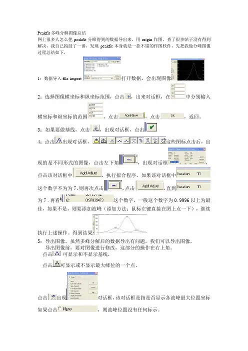
Peakfit多峰分解图像总结网上很多人怎么把peakfit分峰得到的数据导出来,用origin作图,查了很多帖子没有得到解决,我自己捣鼓了一番,发现peakfit本身就是一款不错的作图软件,先把我做分峰图像过程总结如下,1:数据导入file-import-打开数据,会出现图像2:选择图像横坐标和纵坐标范围,点击,出来对话框,在中分别输入横坐标和纵坐标的范围,点击,点击,返回。
3:如果要做基线,点击,出现对话框,点击4:点击出现对话框,这些图标点击后,出现的是不同形式的图像,点击左下角,出现对话框,点击该对话框中,执行拟合程序,如果该对话框中这个数字不为为7,则再次点击,点击,直到为7 .再看这个数字,一般这个数字为0.9996以上为最佳,如果不是,则要添加波峰(添加方法:鼠标左键直接在图上点一下),继续执行上述操作。
得到结果5:导出图像,虽然多峰分解后的数据导出有问题,我们可以导出图像,导出图像前,要对图像进行修改,这部分的操作在右上角。
点击可显示和不显示基线,点击可显示或不显示最大峰位的一个点。
点击出现对话框,该对话框是指是否显示各波峰最大位置坐标如果点击,则波峰位置没有任何标示。
点击可对图背景颜色设计,一般用点击可对字体进行修改,点击可对标题进行修改,点击可对原始数据做的图进行修改点击出现对话框,可对背景是否要格子进行修改,所有以上修改后,都要点击才能保持修改,返回这是你可在图标中选择合适的图像,点击进行拷贝,复制到你要的地方。
以上介绍了分峰与图像导出,但我发现对于图片能够控制的条件很有限,这样导出的图像很丑,长宽比不合理,远不如origin那样灵活可控。
下面将分峰后导出ASCII的步骤列出:分峰完成后点左下角的“preview peak fit”:弹出界面:这个界面上方有一条工具条,跟前面的界面功能一样,这里不再赘述,(最后两个按钮不知道是什么作用,幸好这里用不到~)点击“hide Y2 plot”: (此步骤不是必需的,可省略)然后点左侧的“Export”:数据导出就完成了。
简介:进口调节阀标准、进口调节阀作用、进口调节阀原理、进口调节阀型号德国FIKE菲克阀门进口调节阀用于调节工业自动化过程控制领域中的介质流量、压力、温度、液位等工艺参数。
根据自动化系统中的控制信号,自动调节阀门的开度,从而实现介质流量、压力、温度和液位的调节。
进口调节阀通常由电动执行机构或气动执行机构与阀体两部分共同组成。
直行程主要有直通单座式和直通双座式两种,后者具有流通能力大、不平衡办小和操作稳定的特点,所以通常特别适用于大流量、高压降和泄漏少的场合。
进口调节阀分类进口电动调节阀、进口气动调节阀、进口自力式调节阀、进口温度调节阀、进口流量调节阀、进口单座调节阀、进口双座调节阀、进口角形调节阀进口调节阀流量特性进口调节阀的流量特性,是在阀两端压差保持恒定的条件下,介质流经调节阀的相对流量与它的开度之间关系。
调节阀的流量特性有线性特性,等百分比特性及抛物线特性三种。
调节阀等百分比特性、调节阀线性特性、调节阀抛物线特性。
三种注量特性的意义如下(1)等百分比特性(对数)等百分比特性的相对行程和相对流量不成直线关系,在行程的每一点上单位行程变化所引起的流量的变化与此点的流量成正比,流量变化的百分比是相等的。
所以它的优点是流量小时,流量变化小,流量大时,则流量变化大,也就是在不同开度上,具有相同的调节精度。
(2)线性特性(线性)线性特性的相对行程和相对流量成直线关系。
单位行程的变化所引起的流量变化是不变的。
流量大时,流量相对值变化小,流量小时,则流量相对值变化大。
(3)抛物线特性流量按行程的二方成比例变化,大体具有线性和等百分比特性的中间特性。
从上述三种特性的分析可以看出,就其调节性能上讲,以等百分比特性为最优,其调节稳定,调节性能好。
而抛物线特性又比线性特性的调节性能好,可根据使用场合的要求不同,挑选其中任何一种流量特性。
(4)流量系数Kv进口调节阀的流量系数Kv,是调节阀的重要参数,它反映调节阀通过流体的能力,也就是调节阀的容量。
各位虫友大家好,我是虫友rabbit_he. 今天,我做的语音教程是关于软件PeakFit的入门教程---因为我是学催化专业的,之后会带来它实战XRD、XPS、IR峰的应用语音教程,就没在深究它在其它方面的应用了。
具体大家看我的操作(语音可能不太清楚,又是新手做教程,敬请大家原谅,海涵啊^-^),我先给大家介绍一下peakfit到底能干什么?Peakfit -------- 最佳自动分离、拟合与分析非线性数据软件第一名的非线性尖峰曲线套配软件Peakfit 色层分析及光谱研究软件使用非线性曲线的适当峰值可让您侦测、测定及分析隐藏在未解决峰值数据中的峰值,使用可在屏幕上管控的图形分析方式,省略复杂的数学积分技巧。
在光谱(XRD XPS IR=其它一些光谱数据,据我所知现在有很多人用xpspeak分析xps数据,大家学了这个,你不觉得没有必要单独学它了,嘿嘿),层析,电泳分析时,我们常需要非线性曲线套配,以找出合理的峰值.以前要花许多时间的资料分析工作,现在只要几分钟即可,不管是复杂或噪声多的资料,都有办法帮您处理。
--------------------------------------------------------------------------------。
欢迎访问SYSTAT美国网站:/ ,您可以获得更详尽的信息。
点击下载详细手册:SYSTA T_PDF文件-----它主页的pdf没啥用,就四页,我上传的附件中带了一个从程序中提取出来后的帮助文档,pdf格式,295页,有兴趣的虫友多研究研究。
安装时先正常安装peakfit.exe 安完后,启动程序时会有一界面,上有三个按钮update -----continue-----exit,点击update,之后启动keygen.exe输入注册码就ok啦!!!不注册的话,它有三十天的使用期限,期限一到,你就不能使用了。
----------------------------------------------------------------------------------------------------------------------大家没兴趣的话都不用看这个英文介绍,到实战的时候,我会具体而详细的都讲一下,下面简要的挑几个概念讲一下Peakfit's state - of -the - art nonlinear curve fitting is essential for accurate peak analysis and conclusive findings. PeakFit separates and analyzes nonlinear peak data better, more accurately and more conveniently than your lab instrument. Nonlinear curve fitting is by far the most accurate way to reduce noise and quantify peaks.PeakFit uses three procedures to automatically place hidden peaks, while each is a strong solution, one method may work better with some data sets than the others. The three Procedures are... Residuals - initially places peaks by finding local maxima in a smoothed data streamSecond Derivative - searches for local minima within a smoothed second derivative data stream Deconvolution - uses a Gaussian response function with a Fourier deconvolution/ filtering algorithm.PeakFit helps you separate overlapping peaks by statistically fitting numerous peak functions to one data set, which can help you find even the most obscure patterns in your data. The background can be fit as a separate polynomial(多项式), exponential, logarithmic, hyperbolic(双曲线)or power model. This fitted baseline is then subtracted before peak characterization data (such as areas) is calculated, which gives much more accurate results.PeakFit is the automatic choice for Spectroscopy, Chromatography or Electrophoresis. AI Experts throughout the smoothing options and other parts of the program automatically help you to set many adjustments.PeakFit can even deconvolve your spectral instrument response so that you can analyze your data without the smearing that your instrument introduces. By Using 82 nonlinear peak models to choose from, you're almost guaranteed to find the best equation for your data.PeakFit includes 18 different nonlinear spectral application line shapes, including the Gaussian, the Lorentzian, and the V oigt, and even a Gaussian plus Compton Edge model for fitting Gamma Ray peaks. As a product of the curve fitting process, PeakFit reports amplitude (intensity), area, center and width data for each peak. Overall area is determined by integrating the peak equations in the entire model.The V oigt function is a convolution of both the Gaussian and Lorentzian functions. Most analysis packages that offer a V oigt function use an approximation with very limited precision. PeakFit actually uses a closed-form solution to precisely calculate the function analytically. PeakFit has four different Voigt functions, so you can fit the parameters you're most interested in, including the individual widths of both the Gaussian and Lorentzian components, and also the amplitude and area of the Voigt function. PeakFit's precise calculation of the V oigt function is crucial to the accuracy of your analysis.FeaturesNonlinear Curve FittingFull Graphical Placement of PeaksHighly Advanced Baseline SubtractionPeakFit Saves You Precious Research TimePublication-Quality Graphs and Data OutputPeakFit Offers Sophisticated Data ManipulationPeakFit Automatically Places Peaks in Three WaysData InputData PreparationPeak AutoplacementNon - Linear Curve FittingOutput and Export OptionsFitting Multiple Simultaneous Gaussian FunctionsSYSTEM REQUIREMENTS486 Processor or higherWindows 95 and above8 MB RAM required (12 MB or more recommended)5MB hard disk spaceTOPICSWhy Should You Use Nonlinear Curve Fitting?PeakFit Offers Sophisticated Data ManipulationHighly Advanced Baseline SubtractionFull Graphical Placement of Peaks and...Publication-Quality Graphs and Data OutputPeakFit Saves You Precious Research TimePeakFit Automatically Places Peaks in Three WaysWhy Should You Use Nonlinear Curve Fitting?Nonlinear curve fitting is by far the most accurate way to reduce noise and quantify peaks. Many instruments come with software that only approximates the fitting process by simply integrating the raw data numerically. When there are shouldered, or hidden peaks, a lot of noise, or a significant background signal, this can lead to the wrong results. (For example, a spectroscopy data set may appear to have a peak with a 'raw' amplitude of 4,000 units -- but may have a shoulder peak that distorts the amplitude by 1,500 units! This would be a significant error.)PeakFit helps you separate overlapping peaks by statistically fitting numerous peak functions to one data set, which can help you find even the most obscure patterns in your data. The background can be fit as a separate polynomial, exponential, logarithmic, hyperbolic or power model. This fitted baseline is then subtracted before peak characterization data (such as areas) is calculated, which gives much more accurate results. And any noise (like you get with electrophoretic gels orRaman spectra) that might bias raw data calculations is filtered simply by the nonlinear curve fitting process. Nonlinear curve fitting is essential for accurate peak analysis and accurate research.PeakFit Offers Sophisticated Data ManipulationWith PeakFit's visual FFT filter, you can inspect your data stream in the Fourier domain and zero higher frequency points -- and see your results immediately in the time-domain. This smoothing technique allows for superb noise reduction while maintaining the integrity of the original data stream. PeakFit also includes an automated FFT method as well as Gaussian convolution, the Savitzky-Golay method, and the Loess algorithm for smoothing. AI Experts throughout the smoothing options and other parts of the program automatically help you to set many adjustments. And, PeakFit even has a digital data enhancer, which helps to analyze your sparse data. Only PeakFit offers so many different methods of data manipulation.Click to View Larger ImageHighly Advanced Baseline SubtractionPeakFit's non-parametric baseline fitting routine easily removes the complex background of a DNA electrophoresis sample. PeakFit can also subtract eight other built-in baseline equations, or it can subtract any baseline you've developed and stored in a file.Click to View Larger ImageFull Graphical Placement of PeaksIf PeakFit's auto-placement features fail on extremely complicated or noisy data, you can place and fit peaks graphically with only a few mouse clicks. Each placed function has "anchors" that adjust even the most highly complex functions, automatically changing that function's specific numeric parameters. PeakFit's graphical placement options handle even the most complex peaks as smoothly as Gaussians.Publication-Quality Graphs and Data OutputEvery publication-quality graph (see above) was created using PeakFit's built-in graphic engine -- which now includes print preview and extensive file and clipboard export options. The numerical output is customizable so that you see only the content you want.PeakFit Saves You Precious Research TimeFor most data sets, PeakFit does all the work for you. What once took hours now takes minutes –with only a few clicks of the mouse! It’s so easy that novices can learn how to use PeakFit in no time. And if you have extremely complex or noisy data sets, the sophistication and depth ofPeakFit’s data manipulation techniques is unequaled.PeakFit Automatically Places Peaks in Three WaysPeakFit uses three procedures to automatically place hidden peaks; while each is a strong solution, one method may work better with some data sets than the others.The Residuals procedure initially places peaks by finding local maxima in a smoothed data stream. Hidden peaks are then optionally added where peaks in the residuals occur.The Second Derivative procedure searches for local minima within a smoothed second derivative data stream. These local minima often reveal hidden peaks.The Deconvolution procedure uses a Gaussian response function with a Fourier deconvolution/ filtering algorithm. A successfully deconvolved spec-trum will consist of “sharpened” peaks of equivalent area. The goal is to enhance the hidden peaks so that each represents a local maximum. Built-In Nonlinear Functions (83 total)Spectroscopy (18): Gauss Amp(高斯), Gauss Area, Lorentz Amp, Lorentz Area, V oigt Amp, V oigt Area, Voigt Amp Approx, V oigt Amp G/L, Voigt Area G/l, Gauss Cnstr Amp, Gauss Cnstr Area, Pearson VII Amp, Pearson VII Area, Gauss+Lor Area, Gauss*Lor, Gamma Ray, Compton Edge.Chromatography (8): HVL, NLC, Giddings, EMG, GMG, EMG+GMG, GEMG, GEMG 5-parm.Statistical (31): Log Normal Amp, Log Normal Area, Logistic Amp, Logistic Area, Laplace Amp, Laplace Area, Extr V alue Amp, Extr Value Area, Log Normal-4 Amp, Log Normal-4 Area, Eval4 Amp Tailed, Eval4 Area Tailed, Eval4 Amp Frtd, Eval4 Area Frtd, Gamma Amp, Gamma Area, Inv Gamma Amp, Inv Gamma Area, Weibull Amp, Weibull Area, Error Amp, Error Area, Chi-Sq Amp, Chi-Sq Area, Student t Amp, Student t Area, Beta Amp, Beta Area, F Variance Amp, F Variance Area, Pearson IV.General Peak (12): Erfc Pk, Pulse Pk, LDR Pk, Asym Lgstc Pk, Lgstc pow Pk, Pulse pow Pk, Pulse Wid2 Pk, Intermediate Pk, Sym Dbl Sigmoid, Sym Dbl GaussCum, Asym Dbl Sigmoid, Asym Dbl GaussCum.Transition (14): Sigmoid Asc, Sigmoid Desc, GaussCum Asc, GaussCum Desc, LorentzCum Asc, LorentzCum Desc, LgstcDose Rsp Asc, LgstcDoseRsp Desc, LogNormCum Asc, LogNormCum Desc, ExtrValCum Asc, ExtrValCum Desc, PulseCum Asc, PulseCum Desc.User Defined FunctionsUp to 10 Parameters per function.Up to 15 UDF's active during fit.Estimates can contain formulas and constraints.Extensive mathematical, statistical, Bessel, and logic functions.Baseline Fit and SubtractAutomatic detection of baseline points by constant second derivatives.Real-time Fitting in conjunction with data point selection, deselection.Background Functions (10): Constant, Linear, Progressive Linear, Quadratic, Cubic, Logarithmic, Exponential, Power, Hyperbolic and Non-Parametric.Graphical ReviewComponent and Sum Curve graphs.Residuals Graphs, including Distribution and Stabilized Normal Probability Plots.Confidence and Prediction Intervals.Peak Labels (Amplitude, Center, or Area).Numerical ReviewPeak Characterization data: Center, Amplitude, Integrated Area, Analytical Area, FWHM, FW10, FWBASE, Asymmetry at HM, Asymmetry at 10 percent, First and Second Moments, Column Efficiency and Resolution, Percentage Areas, Overlap Areas.Parameter Statistics: Parameter Values, Confidence Limits (90, 95, 99 percent), t-values, Standard Errors.Fit Statistics: Analysis of Variance, F-statistic, Overall Standard Error, r2 value(回归系数平方和---以后我们使用时重点关注的参数,它值在0-1之间,越接近于1,你的拟合效果越好).Data Statistics: Residual Values, Predicted Y-values, Confidence/Prediction Intervals.PeakFit Offers Sophisticated Data ManipulationHighly Advanced Baseline SubtractionPeakFit Automatically Places Peaks in Three WaysPeakFit Automatically Places Peaks in Three WaysSingle Channel Analysis Fitting Multiple Simultaneous Gaussian FunctionsSingle Channel Analysis Fitting Multiple Simultaneous Gaussian FunctionsSingle Channel Analysis Fitting Multiple Simultaneous Gaussian FunctionsSingle Channel Analysis Fitting Multiple Simultaneous Gaussian Functions下面,我们着重看一下程序界面。
PeakFit软件介绍和特⾊功能peakfit是⼀款⾮常强⼤的数据拟合软件,它的主要功能就是帮助⽤户进⾏数据峰值的分析情况,软件的操作⽅法也是⾮常简单的,只需要将想要统计的数据进⾏⼀个导⼊,然后进⾏分析,软件就会⾃动拟合出各种数据的峰值情况来展现给⽤户们观看,并且⽤户们还可以⾃⼰设置各种参数来进⾏分析,软件的检测结果是⾮常准确的,可以直接导⼊AIA、ascll、Excel等多种格式类型的数据进⾏分析,软件相⽐于其它软件的优势之处就在于其拥有⾮常给⼒的部分重新扫描功能,这样⽤户在⾃由调整设置峰值的数值的时候就不需要全部修改峰值了,节省了⾮常多的时间,提升了⼯作效率,整个⼯作过程中是⾮常的⽅便快捷的,对于那些需要处理数据或者分析数据的⽤户们来说真的⾮常的合适,⼩编在这⾥带来的是peakfit永久破解版,⽤户永久免费使⽤,还有相关的安装教程帮助各位⽤户们来下载使⽤!peakfit是⼀款⾮常强⼤的数据拟合软件,它的主要功能就是帮助⽤户进⾏数据峰值的分析情况,软件的操作⽅法也是⾮常简单的,只需要将想要统计的数据进⾏⼀个导⼊,然后进⾏分析,软件就会⾃动拟合出各种数据的峰值情况来展现给⽤户们观看,并且⽤户们还可以⾃⼰设置各种参数来进⾏分析,软件的检测结果是⾮常准确的,可以直接导⼊AIA、ascll、Excel等多种格式类型的数据进⾏分析,软件相⽐于其它软件的优势之处就在于其拥有⾮常给⼒的部分重新扫描功能,这样⽤户在⾃由调整设置峰值的数值的时候就不需要全部修改峰值了,节省了⾮常多的时间,提升了⼯作效率,整个⼯作过程中是⾮常的⽅便快捷的,对于那些需要处理数据或者分析数据的⽤户们来说真的⾮常的合适,⼩编在这⾥带来的是peakfit永久破解版,⽤户永久免费使⽤,还有相关的安装教程帮助各位⽤户们来下载使⽤!peakfit安装教程1、将下载好的压缩包进⾏解压得到软件安装程序,双击打开2、点击下⼀步开始安装3、这⾥输⼊⽂件夹内的注册信息,点击下⼀步注册安装4、在这⾥可以选择软件的安装⽬录,选择好之后点击下⼀步安装5、稍微等待之后软件会⾃动安装完成,点击完成退出向导即可6、之后双击桌⾯快捷程序即可打开软件7、点击帮助中可以看到软件已经成功激活,如果上述没有激活的话可以使⽤【DAA6CD55-FBFB1907】激活码激活分峰拟合教程⼀、选中拟合谱峰区间1、点击快捷⼯具栏第⼋个按钮,section2、在左侧界⾯中输⼊适当的Xi与Xf值,尽量让谱峰位于图中正中位置,点击applyexisting。
PF解谱软件使用说明1.双击PF图标运行PF.exe,图 1弹出如下PeakFit V4界面:图 22. 关于实验数据文本PF软件所用的数据文本的保存格式应为:“文件名.dat”。
当然数据文本可以先保存在记事本里,然后将其后缀改成”.dat”。
接下来以CO的实验数据“dco30303.dat”为例,讲解数据导入和解谱过程。
3. 导入待解谱的实验数据文本一般有两种数据导入方式:(1)用“File”菜单打开a. 在PeakFit V4界面内,打开菜单栏的“File”以及其下拉菜单中的“import”选项(第一个)。
在弹出的“Read XY Data From File ”对话框内查找你所保存的实验数据文本“dco30303.dat”,得到下图:图 3b. 然后选中并“打开”,这时会弹出“Data Description and Variable Names”对话框。
在“Main Title”一栏里,你可以键入将要生成的实验数据文本的二维图像的名称,比如“dco30303”;在“X Title”或“Y Title”里键入X或Y坐标轴的标识,即相关的物理变量。
图 4c. 之后,点击“OK”,你会得到一张名为“dco30303”的多峰图。
在图的左边有对图像的简单统计分析,包括X、Y变量的极值及其坐标(Min,Max)、区间长度(Range)、中位数(Median)、平均值(Mean)以及曲线和X坐标轴所围区域的面积。
图 5(2) 你也可以在PeakFit V4界面内,使用“ctrl+I”快捷键或点击工具栏的“打开文件夹”(第一个),直接弹出“Read XY Data From File ”对话框,以后的操作和(1)相同,不再赘述!4. 导入数据拟合函数文件点击PeakFit V4界面工具栏里的“U”图标(如图5的红圈所示),会弹出“User Defined Function 1”(图6所示)对话框。
用户在这里有两种方式输入自编的拟合函数对数据进行拟合:(1)请注意此对话框右上角的“Selected UDF”选项,这里有“1”到“15”的函数输入按钮。
计算化学领域一直是一个备受关注的领域,许多科学家和研究人员都在积极探索各种计算方法来解决化学问题。
在这个过程中,peakfit碳谱核磁算双螺旋计算逐渐成为了一个备受瞩目的研究方向。
本文将对peakfit碳谱核磁算双螺旋计算进行深入探讨,并分析其在计算化学领域中的应用和前景。
1. peakfit碳谱核磁算双螺旋计算的基本原理peakfit碳谱核磁算双螺旋计算是一种结合了碳谱核磁共振和双螺旋计算的方法。
在这种方法中,通过对化学物质中产生的谱峰进行分析,可以得到物质的分子结构信息。
利用双螺旋计算的原理,可以模拟和预测分子的构象和性质,从而为化学研究提供了有力的工具和方法。
2. peakfit碳谱核磁算双螺旋计算在化学研究中的应用peakfit碳谱核磁算双螺旋计算在化学研究中有着广泛的应用。
在分子结构的确定中,这种方法可以通过对谱峰的分析来推断分子中的化学键类型和环的结构,从而帮助化学家确定未知化合物的结构。
在分子模拟和设计中,通过双螺旋计算可以模拟分子的构象和性质,为新材料和药物的设计提供了理论依据。
3. peakfit碳谱核磁算双螺旋计算的发展趋势随着化学研究的不断深入和发展,peakfit碳谱核磁算双螺旋计算也在不断地进行改进和完善。
未来,随着计算机技术的进步,计算方法更加高效和精确。
随着化学实验技术的不断革新,可以提供更多更准确的谱峰数据,从而使计算结果更可靠和准确。
4. peakfit碳谱核磁算双螺旋计算在实际应用中的挑战和问题尽管peakfit碳谱核磁算双螺旋计算在理论上具有很大的潜力,但是在实际应用中还存在许多挑战和问题。
谱峰数据的获取和分析本身就是一个复杂的过程,需要高度专业的仪器和技术人员。
在双螺旋计算中,模型的建立和参数的选择也需要经验丰富的研究人员进行指导和解释。
另外,在计算过程中,计算精度和速度也是一个需要不断优化的问题。
5. 总结总体来说,peakfit碳谱核磁算双螺旋计算作为一种有着广阔前景的计算化学方法,它在化学研究和应用中发挥着重要的作用。
peakfit红外分峰拟合峰归属
在红外光谱分析中,常常需要对样品的光谱进行拟合和分峰,以便准确地识别样品中含有的化合物。
而Peakfit红外分峰拟合是一种常用的方法,它可以自动识别样品中的峰,并将其归属于不同的化合物。
作为一种基于非线性最小二乘法的拟合工具,Peakfit可以对红外光谱数据进行高效、准确的分峰和拟合。
它可以自动识别样品中的峰,并根据用户提供的峰形函数进行拟合。
同时,Peakfit还可以进行背景拟合和剪切线去除,进一步提高分析的准确度。
对于拟合过程中出现的峰归属问题,Peakfit提供了多种解决方案。
一种常用的方法是通过峰的位置和峰形状进行识别,并将其与化合物数据库进行比对,以确定峰的归属。
另外,还可以通过添加标准样品进行验证,以进一步提高峰的归属准确度。
总的来说,Peakfit红外分峰拟合是一种高效、准确的红外光谱分析工具,它可以帮助化学研究人员快速、准确地识别样品中的化合物。
- 1 -。
国外织物风格仪KESF和FAST比较研究摘要本文通过对KESF和FAST技术在测试原理和测试结果的比较,分析二者的优缺点,并且结合我国国情得出FAST技术在我国纺织品行业推广的现实意义。
关键词:织物风格KESF FAST测试原理前言织物风格,作为织品本身的物理和机械特征与人的主观感受相互作用的产物,是一个复杂,抽象的评价指标。
但同时,它在反映织品外观美感和穿用舒适性方面又是一个重要的依据。
初期的织品风格评定往往单纯借助于视觉和触觉,这种主观评定容易受人为因素影响,不够稳定。
为了找到统一的定量化评价织物的标准,科研工作者作了大量的研究工作。
目前较成功的、也是有代表性的测试系统是KESF(Kawabata织物风格评价系统)和FAST(Fabric assurance by testing simple testing),因两者的测试原理有所差异,认清二者的差别点,对于实际应用有很强的指导作用。
1测试原理的差别FAST测试法的基本原理FAST(织物质地简易测试法)是澳大利亚工业和科学院研制的一套毛织物特性测试系统,用来测定织物特性对裁剪缝制性能及成衣外观的影响。
该测试系统是专为毛织物生产、整理及服装制造厂质量管理而设计。
FAST系统属于分项式多机台型测试仪,它包括三台仪器和一种试验方法,即FAST—1压缩仪、FAST—2弯曲仪、FAST—3拉伸仪和FAST—4尺寸稳定性测试方法。
通过测试织物的压缩、弯曲、拉伸、剪切等四项基本力学性能和尺寸稳定性,并绘出相应的“织物指纹图”,用来评价织物的外观、手感和预测织物的可缝性、成形性。
KESF测试法的基本原理KESF,也称川端评价系统(Kawabata’s Evluation system),是以川端季雄为首的日本织物风格评价和标准化委员会(HESC)研制的一整套织物风格测试仪。
川端法把织物风格分为三个层次:1.2.1力学量:是利用KES—F风格仪对织物测试获得的拉伸、弯曲、剪切、压缩、厚度及重量,以及表面性质的16个力学参数.1.2.2 基本风格:以川端季雄为首的日本织物风格评价和标准化委员会(HESC)对各种风格特征感觉进行了统一定义,提出了若干基本风格.例如:男式冬季外衣料有三种基本风格:硬挺度;光滑度;丰满度。
各种数据处理软件Contents:1.正交设计助手II v3.1是一款针对正交实验设计及结果分析而制作的专业共享软件。
正交设计方法是我们常用的实验设计方法,它让我们以较少的实验次数得到科学的实验结论。
但是我们经常不得不重复一些机械的工作,比如填实验安排表,计算各个水平的均值等等。
正交设计助手可以帮助您完成这些繁琐的工作。
2.PeakFit 4.12 Demo自动分离、拟合与分析非线性数据软件。
分析非线性数据,进行曲线作更方便,更精确。
有时间限制补丁程序!可长期使用!3.GraphPad PRISM4.0 demo著名的数据处理软件,用来进行统计、曲线拟合以及作图。
4.SigmaStat 3.5 Demo是一个易于使用的智能统计软件,尤其适合对统计知识了解不多的人使用,它具有一个“专家系统”,引导你对数据进行统计分析。
5.数据作图助手II v2.1_A是一款用于对实验结果进行数据分析和作图的专业软件。
它可满足您根据实验数据作出经验曲线,或以平滑曲线联结各数据点的要求。
支持三次样条插值算法、最小二乘法直线拟合算法、可化为直线方程处理的特殊函数方程拟合算法以及一元多项式回归算法。
6.CurveExpert 1.38对ELISA标准曲线拟合头痛吗?实际上,不只是ELISA标准曲线拟合,其它各种有关的实验数据分析,都可以应用CurveExpert进行数据分析。
7.NoSA5 2005.6.13版中文统计软件。
覆盖了绝大部分常用的统计分析方法,嵌入了当代数据处理技术,能满足从事各类研究的专家、学者对数据作统计分析的需要,是各专业研究生、本科生统计学教学的优秀课件。
8.DRS 2005依据"最小三乘法"编制的数据回归分析软件;它使得一元线性、多元线性、一元非线性以至多元非线性的数据回归,计算更简单结果更准确。
各位虫友大家好,我是虫友rabbit_he. 今天,我做的语音教程是关于软件PeakFit的入门教程---因为我是学催化专业的,之后会带来它实战XRD、XPS、IR峰的应用语音教程,就没在深究它在其它方面的应用了。
具体大家看我的操作(语音可能不太清楚,又是新手做教程,敬请大家原谅,海涵啊^-^),我先给大家介绍一下peakfit到底能干什么?Peakfit -------- 最佳自动分离、拟合与分析非线性数据软件第一名的非线性尖峰曲线套配软件Peakfit 色层分析及光谱研究软件使用非线性曲线的适当峰值可让您侦测、测定及分析隐藏在未解决峰值数据中的峰值,使用可在屏幕上管控的图形分析方式,省略复杂的数学积分技巧。
在光谱(XRD XPS IR=其它一些光谱数据,据我所知现在有很多人用xpspeak分析xps数据,大家学了这个,你不觉得没有必要单独学它了,嘿嘿),层析,电泳分析时,我们常需要非线性曲线套配,以找出合理的峰值.以前要花许多时间的资料分析工作,现在只要几分钟即可,不管是复杂或噪声多的资料,都有办法帮您处理。
--------------------------------------------------------------------------------。
欢迎访问SYSTAT美国网站:/ ,您可以获得更详尽的信息。
点击下载详细手册:SYSTA T_PDF文件-----它主页的pdf没啥用,就四页,我上传的附件中带了一个从程序中提取出来后的帮助文档,pdf格式,295页,有兴趣的虫友多研究研究。
安装时先正常安装peakfit.exe 安完后,启动程序时会有一界面,上有三个按钮update -----continue-----exit,点击update,之后启动keygen.exe输入注册码就ok啦!!!不注册的话,它有三十天的使用期限,期限一到,你就不能使用了。
----------------------------------------------------------------------------------------------------------------------大家没兴趣的话都不用看这个英文介绍,到实战的时候,我会具体而详细的都讲一下,下面简要的挑几个概念讲一下Peakfit's state - of -the - art nonlinear curve fitting is essential for accurate peak analysis and conclusive findings. PeakFit separates and analyzes nonlinear peak data better, more accurately and more conveniently than your lab instrument. Nonlinear curve fitting is by far the most accurate way to reduce noise and quantify peaks.PeakFit uses three procedures to automatically place hidden peaks, while each is a strong solution, one method may work better with some data sets than the others. The three Procedures are... Residuals - initially places peaks by finding local maxima in a smoothed data streamSecond Derivative - searches for local minima within a smoothed second derivative data stream Deconvolution - uses a Gaussian response function with a Fourier deconvolution/ filtering algorithm.PeakFit helps you separate overlapping peaks by statistically fitting numerous peak functions to one data set, which can help you find even the most obscure patterns in your data. The background can be fit as a separate polynomial(多项式), exponential, logarithmic, hyperbolic(双曲线)or power model. This fitted baseline is then subtracted before peak characterization data (such as areas) is calculated, which gives much more accurate results.PeakFit is the automatic choice for Spectroscopy, Chromatography or Electrophoresis. AI Experts throughout the smoothing options and other parts of the program automatically help you to set many adjustments.PeakFit can even deconvolve your spectral instrument response so that you can analyze your data without the smearing that your instrument introduces. By Using 82 nonlinear peak models to choose from, you're almost guaranteed to find the best equation for your data.PeakFit includes 18 different nonlinear spectral application line shapes, including the Gaussian, the Lorentzian, and the V oigt, and even a Gaussian plus Compton Edge model for fitting Gamma Ray peaks. As a product of the curve fitting process, PeakFit reports amplitude (intensity), area, center and width data for each peak. Overall area is determined by integrating the peak equations in the entire model.The V oigt function is a convolution of both the Gaussian and Lorentzian functions. Most analysis packages that offer a V oigt function use an approximation with very limited precision. PeakFit actually uses a closed-form solution to precisely calculate the function analytically. PeakFit has four different Voigt functions, so you can fit the parameters you're most interested in, including the individual widths of both the Gaussian and Lorentzian components, and also the amplitude and area of the Voigt function. PeakFit's precise calculation of the V oigt function is crucial to the accuracy of your analysis.FeaturesNonlinear Curve FittingFull Graphical Placement of PeaksHighly Advanced Baseline SubtractionPeakFit Saves You Precious Research TimePublication-Quality Graphs and Data OutputPeakFit Offers Sophisticated Data ManipulationPeakFit Automatically Places Peaks in Three WaysData InputData PreparationPeak AutoplacementNon - Linear Curve FittingOutput and Export OptionsFitting Multiple Simultaneous Gaussian FunctionsSYSTEM REQUIREMENTS486 Processor or higherWindows 95 and above8 MB RAM required (12 MB or more recommended)5MB hard disk spaceTOPICSWhy Should You Use Nonlinear Curve Fitting?PeakFit Offers Sophisticated Data ManipulationHighly Advanced Baseline SubtractionFull Graphical Placement of Peaks and...Publication-Quality Graphs and Data OutputPeakFit Saves You Precious Research TimePeakFit Automatically Places Peaks in Three WaysWhy Should You Use Nonlinear Curve Fitting?Nonlinear curve fitting is by far the most accurate way to reduce noise and quantify peaks. Many instruments come with software that only approximates the fitting process by simply integrating the raw data numerically. When there are shouldered, or hidden peaks, a lot of noise, or a significant background signal, this can lead to the wrong results. (For example, a spectroscopy data set may appear to have a peak with a 'raw' amplitude of 4,000 units -- but may have a shoulder peak that distorts the amplitude by 1,500 units! This would be a significant error.)PeakFit helps you separate overlapping peaks by statistically fitting numerous peak functions to one data set, which can help you find even the most obscure patterns in your data. The background can be fit as a separate polynomial, exponential, logarithmic, hyperbolic or power model. This fitted baseline is then subtracted before peak characterization data (such as areas) is calculated, which gives much more accurate results. And any noise (like you get with electrophoretic gels orRaman spectra) that might bias raw data calculations is filtered simply by the nonlinear curve fitting process. Nonlinear curve fitting is essential for accurate peak analysis and accurate research.PeakFit Offers Sophisticated Data ManipulationWith PeakFit's visual FFT filter, you can inspect your data stream in the Fourier domain and zero higher frequency points -- and see your results immediately in the time-domain. This smoothing technique allows for superb noise reduction while maintaining the integrity of the original data stream. PeakFit also includes an automated FFT method as well as Gaussian convolution, the Savitzky-Golay method, and the Loess algorithm for smoothing. AI Experts throughout the smoothing options and other parts of the program automatically help you to set many adjustments. And, PeakFit even has a digital data enhancer, which helps to analyze your sparse data. Only PeakFit offers so many different methods of data manipulation.Click to View Larger ImageHighly Advanced Baseline SubtractionPeakFit's non-parametric baseline fitting routine easily removes the complex background of a DNA electrophoresis sample. PeakFit can also subtract eight other built-in baseline equations, or it can subtract any baseline you've developed and stored in a file.Click to View Larger ImageFull Graphical Placement of PeaksIf PeakFit's auto-placement features fail on extremely complicated or noisy data, you can place and fit peaks graphically with only a few mouse clicks. Each placed function has "anchors" that adjust even the most highly complex functions, automatically changing that function's specific numeric parameters. PeakFit's graphical placement options handle even the most complex peaks as smoothly as Gaussians.Publication-Quality Graphs and Data OutputEvery publication-quality graph (see above) was created using PeakFit's built-in graphic engine -- which now includes print preview and extensive file and clipboard export options. The numerical output is customizable so that you see only the content you want.PeakFit Saves You Precious Research TimeFor most data sets, PeakFit does all the work for you. What once took hours now takes minutes –with only a few clicks of the mouse! It’s so easy that novices can learn how to use PeakFit in no time. And if you have extremely complex or noisy data sets, the sophistication and depth ofPeakFit’s data manipulation techniques is unequaled.PeakFit Automatically Places Peaks in Three WaysPeakFit uses three procedures to automatically place hidden peaks; while each is a strong solution, one method may work better with some data sets than the others.The Residuals procedure initially places peaks by finding local maxima in a smoothed data stream. Hidden peaks are then optionally added where peaks in the residuals occur.The Second Derivative procedure searches for local minima within a smoothed second derivative data stream. These local minima often reveal hidden peaks.The Deconvolution procedure uses a Gaussian response function with a Fourier deconvolution/ filtering algorithm. A successfully deconvolved spec-trum will consist of “sharpened” peaks of equivalent area. The goal is to enhance the hidden peaks so that each represents a local maximum. Built-In Nonlinear Functions (83 total)Spectroscopy (18): Gauss Amp(高斯), Gauss Area, Lorentz Amp, Lorentz Area, V oigt Amp, V oigt Area, Voigt Amp Approx, V oigt Amp G/L, Voigt Area G/l, Gauss Cnstr Amp, Gauss Cnstr Area, Pearson VII Amp, Pearson VII Area, Gauss+Lor Area, Gauss*Lor, Gamma Ray, Compton Edge.Chromatography (8): HVL, NLC, Giddings, EMG, GMG, EMG+GMG, GEMG, GEMG 5-parm.Statistical (31): Log Normal Amp, Log Normal Area, Logistic Amp, Logistic Area, Laplace Amp, Laplace Area, Extr V alue Amp, Extr Value Area, Log Normal-4 Amp, Log Normal-4 Area, Eval4 Amp Tailed, Eval4 Area Tailed, Eval4 Amp Frtd, Eval4 Area Frtd, Gamma Amp, Gamma Area, Inv Gamma Amp, Inv Gamma Area, Weibull Amp, Weibull Area, Error Amp, Error Area, Chi-Sq Amp, Chi-Sq Area, Student t Amp, Student t Area, Beta Amp, Beta Area, F Variance Amp, F Variance Area, Pearson IV.General Peak (12): Erfc Pk, Pulse Pk, LDR Pk, Asym Lgstc Pk, Lgstc pow Pk, Pulse pow Pk, Pulse Wid2 Pk, Intermediate Pk, Sym Dbl Sigmoid, Sym Dbl GaussCum, Asym Dbl Sigmoid, Asym Dbl GaussCum.Transition (14): Sigmoid Asc, Sigmoid Desc, GaussCum Asc, GaussCum Desc, LorentzCum Asc, LorentzCum Desc, LgstcDose Rsp Asc, LgstcDoseRsp Desc, LogNormCum Asc, LogNormCum Desc, ExtrValCum Asc, ExtrValCum Desc, PulseCum Asc, PulseCum Desc.User Defined FunctionsUp to 10 Parameters per function.Up to 15 UDF's active during fit.Estimates can contain formulas and constraints.Extensive mathematical, statistical, Bessel, and logic functions.Baseline Fit and SubtractAutomatic detection of baseline points by constant second derivatives.Real-time Fitting in conjunction with data point selection, deselection.Background Functions (10): Constant, Linear, Progressive Linear, Quadratic, Cubic, Logarithmic, Exponential, Power, Hyperbolic and Non-Parametric.Graphical ReviewComponent and Sum Curve graphs.Residuals Graphs, including Distribution and Stabilized Normal Probability Plots.Confidence and Prediction Intervals.Peak Labels (Amplitude, Center, or Area).Numerical ReviewPeak Characterization data: Center, Amplitude, Integrated Area, Analytical Area, FWHM, FW10, FWBASE, Asymmetry at HM, Asymmetry at 10 percent, First and Second Moments, Column Efficiency and Resolution, Percentage Areas, Overlap Areas.Parameter Statistics: Parameter Values, Confidence Limits (90, 95, 99 percent), t-values, Standard Errors.Fit Statistics: Analysis of Variance, F-statistic, Overall Standard Error, r2 value(回归系数平方和---以后我们使用时重点关注的参数,它值在0-1之间,越接近于1,你的拟合效果越好).Data Statistics: Residual Values, Predicted Y-values, Confidence/Prediction Intervals.PeakFit Offers Sophisticated Data ManipulationHighly Advanced Baseline SubtractionPeakFit Automatically Places Peaks in Three WaysPeakFit Automatically Places Peaks in Three WaysSingle Channel Analysis Fitting Multiple Simultaneous Gaussian FunctionsSingle Channel Analysis Fitting Multiple Simultaneous Gaussian FunctionsSingle Channel Analysis Fitting Multiple Simultaneous Gaussian FunctionsSingle Channel Analysis Fitting Multiple Simultaneous Gaussian Functions下面,我们着重看一下程序界面。