neural network identification 神经网络系统辨识外文文献3
- 格式:pdf
- 大小:3.75 MB
- 文档页数:11

利用Matlab进行系统辨识的技术方法一、引言系统辨识是研究系统动态特性的一个重要方法,它广泛应用于控制系统、信号处理、通信等领域。
利用Matlab进行系统辨识能够实现快速、准确的模型建立和参数估计。
本文将介绍在Matlab环境下常用的系统辨识技术方法及其应用。
二、系统辨识的基本概念系统辨识是通过对系统的输入和输出信号进行观测和分析,以推断系统的结构和参数。
一般来说,系统辨识包括建立数学模型、估计系统参数和进行模型验证三个步骤。
1. 建立数学模型建立数学模型是系统辨识的第一步,它是描述系统行为的数学表达式。
常用的数学模型包括线性模型、非线性模型和时变模型等。
2. 估计系统参数在建立了数学模型之后,需要通过对实验数据的分析,估计出系统的参数。
参数估计可以通过最小二乘法、极大似然估计法等方法实现。
3. 模型验证模型验证是为了确定估计得到的系统模型是否准确。
常用的方法有经验验证、残差分析、模型检验等。
三、常用的系统辨识技术方法1. 线性参数模型线性参数模型是最常用的系统辨识方法之一。
它假设系统具有线性特性,并通过估计线性模型的参数来描述系统。
在Matlab中,可以使用函数"arx"进行线性参数模型的辨识。
2. 神经网络模型神经网络模型是一种非线性模型,它通过人工神经元的连接权值来描述系统行为。
在Matlab中,可以使用"nlarx"函数进行神经网络模型的辨识。
3. 系统辨识工具箱Matlab提供了丰富的系统辨识工具箱,包括System Identification Toolbox和Neural Network Toolbox等。
这些工具箱提供了各种方法和函数,方便用户进行系统辨识分析。
四、利用Matlab进行系统辨识的应用案例1. 系统辨识在控制系统中的应用系统辨识在控制系统中具有广泛的应用,如无人机控制、机器人控制等。
通过对系统进行辨识,可以建立准确的数学模型,并用于控制器设计和系统优化。
试论述神经网络系统建模的几种基本方法。
利用BP 网络对以下非线性系统进行辨识。
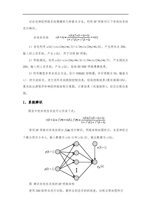
非线性系统22()(2(1)1)(1)()1()(1)y k y k y k u k y k y k -++=+++-1)首先利用u(k)=sin(2*pi*k/3)+1/3*sin(2*pi*k/6),产生样本点500,输入到上述系统,产生y(k), 用于训练BP 网络;2)网络测试,利用u(k)=sin(2*pi*k/4)+1/5*sin(2*pi*k/7), 产生测试点200,输入到上述系统,产生y(k), 检验BP/RBF 网络建模效果。
3)利用模型参考自适应方法,设计NNMARC 控制器,并对周期为50,幅值为+/- 的方波给定,进行闭环系统跟踪控制仿真,检验控制效果(要求超调<5%)。
要求给出源程序和神经网络结构示意图,计算结果(权值矩阵),动态过程仿真图。
1、系统辨识题目中的非线性系统可以写成下式:22()(2(1)1)(1)()();()1()(1)y k y k y k f u k f y k y k -++=•+•=++- 使用BP 网络对非线性部分()f •进行辨识,网络结构如图所示,各层神经元个数分别为2-8-1,输入数据为y(k-1)和y(k-2),输出数据为y(k)。
图 辨识非线性系统的BP 网络结构使用500组样本进行训练,最终达到设定的的误差,训练过程如图所示图网络训练过程使用200个新的测试点进行测试,得到测试网络输出和误差结果分别如下图,所示。
从图中可以看出,相对训练数据而言,测试数据的辨识误差稍微变大,在±0.06范围内,拟合效果还算不错。
图使用BP网络辨识的测试结果图使用BP网络辨识的测试误差情况clear all;close all;%% 产生训练数据和测试数据U=0; Y=0; T=0;u_1(1)=0; y_1(1)=0; y_2(1)=0;for k=1:1:500 %使用500个样本点训练数据U(k)=sin(2*pi/3*k) + 1/3*sin(2*pi/6*k);T(k)= y_1(k) * (2*y_2(k) + 1) / (1+ y_1(k)^2 + y_2(k)^2); %对应目标值Y(k) = u_1(k) + T(k); %非线性系统输出,用于更新y_1if k<500u_1(k+1) = U(k); y_2(k+1) = y_1(k); y_1(k+1) = Y(k); endendy_1(1)=; y_1(2)=0;y_2(1)=0; y_2(2)=; y_2(3)=0; %为避免组合后出现零向量,加上一个很小的数X=[y_1;y_2];save('traindata','X','T');clearvars -except X T ; %清除其余变量U=0; Y=0; Tc=0;u_1(1)=0; y_1(1)=0; y_2(1)=0;for k=1:1:200 %使用500个样本点训练数据U(k)=sin(2*pi/4*k) + 1/5*sin(2*pi/7*k); %新的测试函数Y(k) = u_1(k) + y_1(k) * (2*y_2(k) + 1) / (1+ y_1(k)^2 + y_2(k)^2); if k<200u_1(k+1) = U(k); y_2(k+1) = y_1(k); y_1(k+1) = Y(k); endendTc=Y; Uc=u_1;y_1(1)=; y_1(2)=0;y_2(1)=0; y_2(2)=; y_2(3)=0; %为避免组合后出现零向量,加上一个很小的数Xc=[y_1;y_2];save('testdata','Xc','Tc','Uc'); %保存测试数据clearvars -except Xc Tc Uc ; %清除其余变量,load traindata; load testdata; %加载训练数据和测试数据%% 网络建立与训练[R,Q]= size(X); [S,~]= size(T); [Sc,Qc]= size(Tc);Hid_num = 8; %隐含层选取8个神经元较合适val_iw =rands(Hid_num,R); %隐含层神经元的初始权值val_b1 =rands(Hid_num,1); %隐含层神经元的初始偏置val_lw =rands(S,Hid_num); %输出层神经元的初始权值val_b2 =rands(S,1); %输出层神经元的初始偏置net=newff(X,T,Hid_num); %建立BP神经网络,使用默认参数 %设置训练次数= 50;%设置mean square error,均方误差,%设置学习速率{1,1}=val_iw; %初始权值和偏置{2,1}=val_lw;{1}=val_b1;{2}=val_b2;[net,tr]=train(net,X,T); %训练网络save('aaa', 'net'); %将训练好的网络保存下来%% 网络测试A=sim(net,X); %测试网络E=T-A; %测试误差error = sumsqr(E)/(S*Q) %测试结果的的MSEA1=sim(net,Xc); %测试网络Yc= A1 + Uc;E1=Tc-Yc; %测试误差error_c = sumsqr(E1)/(Sc*Qc) %测试结果的的MSEfigure(1);plot(Tc,'r');hold on;plot(Yc,'b'); legend('exp','act'); xlabel('test smaple'); ylabel('output') figure(2); plot(E1);xlabel('test sample'); ylabel('error')2、MRAC 控制器被控对象为非线性系统:22()(2(1)1)(1)()();()1()(1)y k y k y k f u k f y k y k -++=•+•=++- 由第一部分对()f •的辨识结果,可知该非线性系统的辨识模型为:(1)[(),(1)]()I p y k N y k y k u k +=-+可知u(k)可以表示为(1)p y k +和(),(1)y k y k -的函数,因此可使用系统的逆模型进行控制器设计。

使用Matlab进行非线性系统辨识与控制的技巧在控制系统领域,非线性系统一直是研究的重点和难点之一。
与线性系统不同,非线性系统具有复杂的动力学特性和响应行为,给系统的建模、辨识和控制带来了挑战。
然而,随着计算机技术的快速发展,现在可以利用强大的软件工具如Matlab来进行非线性系统辨识与控制的研究。
本文将分享一些使用Matlab进行非线性系统辨识与控制的技巧,希望对相关研究人员有所帮助。
一、非线性系统辨识非线性系统辨识是指通过实验数据来确定系统的数学模型,以描述系统的动态行为。
在非线性系统辨识中,最常用的方法是基于系统响应的模型辨识技术。
这种方法通常包括以下几个步骤:1. 数据采集和预处理:首先,需要采集实验数据以用于系统辨识。
在数据采集过程中,应尽量减小噪声的影响,并确保数据的可靠性。
然后,对采集到的数据进行预处理,如滤波、采样等,以消除噪声和干扰。
2. 模型结构选择:在进行非线性系统辨识时,应选择合适的模型结构来描述系统的动态特性。
常见的模型结构包括非线性自回归移动平均模型(NARMA),广义回归神经网络(GRNN)等。
选择合适的模型结构对于准确地描述系统非线性特性至关重要。
3. 参数估计:根据选定的模型结构,使用最小二乘法或其他参数估计算法来估计模型的参数。
MATLAB提供了多种估计算法和工具箱,如系统辨识工具箱(System Identification Toolbox)等,可方便地进行参数估计。
4. 模型验证与评估:在参数估计完成后,应对辨识的模型进行验证和评估。
常用的方法是计算模型的均方根误差(RMSE)和决定系数(R-squared),进一步提高模型的准确性和可靠性。
二、非线性系统控制非线性系统控制是指通过设计控制策略来实现对非线性系统的稳定和性能要求。
与非线性系统辨识类似,非线性系统控制也可以利用Matlab进行研究和设计。
以下是一些常用的非线性系统控制技巧:1.反馈线性化控制:线性化是将非线性系统近似为线性系统的一种方法。
MATLAB中常见的自动化建模方法介绍随着科技的不断进步,自动化建模在各个领域中变得越来越重要。
MATLAB作为一种强大的数学建模与仿真工具,为研究人员和工程师们提供了许多自动化建模方法。
本文将介绍几种常见的MATLAB中的自动化建模方法,包括系统辨识、机器学习和优化方法。
一、系统辨识系统辨识是在无法直接获得系统模型的情况下,通过对系统输入和输出数据的观测来估计系统模型。
MATLAB提供了多种用于系统辨识的函数和工具箱,其中最常用的是System Identification Toolbox。
System Identification Toolbox提供了参数估计、模型结构选择和模型验证等功能。
在MATLAB中,使用系统辨识工具箱进行模型辨识一般包括以下步骤:收集系统输入和输出数据、选择适当的模型结构、参数估计和模型验证。
通过这些步骤,研究人员可以获得一个能够准确描述系统动态特性的模型。
二、机器学习机器学习是一种通过让计算机从数据中学习,并且在新的数据上做出预测或决策的方法。
在MATLAB中,有多种机器学习算法可供选择,包括支持向量机(SVM)、人工神经网络(ANN)和决策树等。
支持向量机是一种基于统计学习理论的二分类器,其主要思想是通过在高维特征空间中找到一个最优超平面来实现数据分类。
MATLAB中的Support Vector Machines Toolbox提供了一系列用于支持向量机模型的训练和应用的函数。
人工神经网络是一种模拟人脑神经元网络的算法,它可以通过学习样本数据来进行分类、回归、聚类等任务。
MATLAB中的Neural Network Toolbox提供了一系列用于构建、训练和应用神经网络的函数和工具。
决策树是一种通过对数据进行分割来实现分类的方法。
决策树模型通过一系列的判定条件将数据分为不同的类别。
在MATLAB中,可以利用Classification Learner App来构建和训练决策树模型,同时还可利用TreeBagger函数进行随机森林模型的构建和训练。
神经网络辨识的液压挖掘机 LPV 模型邵辉;胡艳丽;洪雪梅;王飞【摘要】A linear parameter varying model is proposed based on neural network identification for building the hydraulic excavator boom model.The model of the joint angle is obtained based on the first-order plus dead time model of the joint velocity at each working-point.Depending on scheduling variable characteristics,the LPV model parameters are identified by using neural network,and the global LPV model of the excavator boom in the workspace is designed.The simulations and experiments indicate the accuracy of the model and the validity of the method.%针对液压挖掘机动臂关节的非线性建模问题,提出一种基于神经网络的线性变参数(LPV)模型的辨识方法。
在各个工作点处根据其关节速度的一阶惯性加延迟模型,获得其关节角度模型;结合调度变量特性,采用神经网络辨识出 LPV 模型的参数,设计出挖掘机动臂在全局工作范围的 LPV 模型。
通过仿真实验,验证了该方法的有效性和模型的准确性。
【期刊名称】《华侨大学学报(自然科学版)》【年(卷),期】2016(000)001【总页数】5页(P43-47)【关键词】液压挖掘机;动臂关节;神经网络;线性变参数;辨识【作者】邵辉;胡艳丽;洪雪梅;王飞【作者单位】华侨大学信息科学与工程学院,福建厦门 361021;华侨大学信息科学与工程学院,福建厦门 361021;华侨大学信息科学与工程学院,福建厦门361021;华侨大学信息科学与工程学院,福建厦门 361021【正文语种】中文【中图分类】TP273液压挖掘机是结构最复杂、用途最广泛的工程机械之一.目前,大部分液压挖掘机属手动控制,它操作速度慢,效率低,无法应对相对危险的环境[1].因此,实现挖掘机的自动控制是提高效率和安全性的必要途径.对复杂的非线性系统,线性建模方法[2]在非线性因数变化很大时并不适用,而现有的非线性建模方法如机理模型[3]、Volterra级数[4]、非线性ARMAX[5]、Wiener模型[6]等也存在着很多缺陷.最大的问题是非线性过程的复杂性和辨识的高成本.因此,需要寻找一种更好的、低成本的非线性建模方法.神经网络的线性变参数(linear parameter varying,LPV)是Shamma等[7]在研究增益调度控制时首先引入的.对于大部分具有非线性特性的工业过程,其系统并不是在整个操作域内随机无序的进行,而是存在一个与系统动态特性相关的调度变量.而LPV系统的动态特性依赖实时可测的外部参数,其调度参数反映了系统的非线性特性或时变特性,根据调度变量建立系统的LPV模型可以满足系统后继的控制要求.由一个非线性系统得到其LPV模型有2种方法:基于系统动态方程的分析法[8]和基于系统输入输出的实验法[9],实验法常用于辨识LPV的黑箱模型[10].为了辨识系统模型,需要进一步将其参数化,文献[11-13]对此进行了大量的研究,多是将过程模型参数用调度变量的非线性函数表示,采用递归最小二乘法估计模型参数,得到LPV模型.由于调度变量高度的相互依存性,相互之间的函数关系并不明确,且考虑到神经网络可以快速有效地辨识多输入多输出的高度非线性系统.因此,本文采用实验法,提出了基于神经网络的LPV模型的非线性辨识方法.液压挖掘机控制系统是指对发动机、液压泵、多路换向阀和执行元件(液压缸、液压马达)等动力系统进行控制的系统[2],如图1所示.若要对挖掘机进行准确的控制,则必须建立其准确的模型.选取挖掘机的动臂关节,对其进行合理的建模.在单一工作点时,根据工程简化,其阀门开度与动臂关节速度之间是一阶惯性加延迟系统,则阀门开度与关节角度之间的传递函数可以表示为式(1)中包括3个参数依赖系统:系统的稳态增益K;二阶系统的时间常数T;延迟量τ.整个系统是典型的非线性时变系统,K,T,τ分别是关于系统调度变量的函数,均受阀门开度、动臂位置及其运动方向的影响.系统通过阀门开度将泵排出的液压油提供到各元件,使挖掘机完成各项工作,而挖掘机动臂的运动方向及其位置的及时反馈也会驱使挖掘机分流阀动作,使挖掘机在理想的工作面上工作.选择阀门开度、动臂运动方向及其角度作为系统的调度变量.则系统可表示为式(2)中:,w是系统的工作点;η是阀门开度,范围是[ηmin,ηmax];θ是挖掘机动臂的角度,范围是[θmin,θmax];是动臂运动速率,令其表示运动方向,范围是max];而T(w),K(w),τ(w)分别是系统的时间常量、稳态增益及延迟量,也是系统需要辨识的参数集.选用两层前馈神经网络.系统的调度变量阀门开度η,角度θ及运动方向作为神经网络的输入值;系统数学模型参数集稳态增益K(w),时间常数T(w),延迟量τ(w)则作为神经网络的预测输出值,如图2所示.若Ui是输入层节点i的输出,Uk是输出层节点k的输出,Uj是隐含层节点j的输出,则隐含层的第j个节点的输入表示为第j个节点的输出为式(4)中:f(Up,j)为节点激励函数.第j个节点的输出Uj将通过加权系数j,k向前传播到第k个节点,输出层第k个节点的总输入为式(5)中:q为隐含层节点数.则输出层第k个节点的实际网络输出为使用神经网络预测,首先要训练网络,通过训练使网络具有联想记忆和预测能力,有以下6个步骤.步骤1 网络初始化.步骤2 提供训练集.根据调度变量选择工作点测试数据.输入矢量为),期望输出矢量为D=(K,T,τ).步骤3 计算实际输出.步骤4 根据网络预测输出与期望输出,计算网络预测误差.步骤5 更新权值.步骤6 判断算法是否结束,若没有,则返回步骤2.通过对实验数据的多次训练,神经网络达到了理想的效果.采用12 t,挖掘能力0.52 m3的ZAXIS-120型日立挖掘机上的实际数据.针对挖掘机的动臂,在MATLAB/Simulink中建立仿真模型.在操作范围内,即当η∈[0%,100%],θ∈[-70.5°,44.75°],(基于挖掘机基坐标或(令1为方向向上,-1为方向向下)时,选取若干个典型工作点.根据挖掘机提取的数据(部分),如表1所示.表1中:n为实验次数;τ,K,T为近似数值.表1中:测定位姿为挖掘机动臂关节所在位姿的角度,其中,位姿No.1是动臂关节运动到最高极限70.5°角,位姿No.2是运动到水平10.5°角.选择典型工作点采集数据并建立神经网络,经过多次训练,结果如图3所示.从图3可以看出:神经网络具有较高的拟合能力.在已完成神经网络的基础上,于 Matlab/Simulink中建立挖掘机的仿真模型.对挖掘机动臂在开度为100%,从位姿No.1运动到位姿No.2,以及开度为43.75%和31.25%时,从位姿No.2运动到位姿No.1时的运动情况进行阶跃、正弦响应实验仿真,结果如图4所示.由图4比较分析可知:该LPV模型能够很好地逼近真实过程;因为调度变量的全局性,该LPV模型可以模拟系统在整个工作范围内的活动,节省了工作量.为了简化模型并降低成本,提出一种基于神经网络的LPV辨识方法.该方法建立在具有简单结构的数学模型上,结合系统的非线性时变特性,通过神经网络建立调度变量与辨识参数之间的联系.通过仿真实验,得到以下2点结论.1) 引入神经网络,辨识出动态模型参数,能够简单快速地构建系统模型,并在全局范围内有效.2) 基于神经网络的LPV模型结构简单,保证了后继的控制器设计简单可行.【相关文献】[1]LI Bo,YAN Jun,GUO Gang,et al.High performance control of hydraulic excavator based on f uzzy-PI soft-switch controller[C]∥IEEE International Conference on Computer Science and Automation Engineering.Shanghai:IEEE Press,2011:676-679.[2]LU Guangming,SUN Lining,XU Yuan.BP network control over the track of working device of hydraulic excavator[J].Chinese Journal of Mechanical Engineering,2005,41(5):199-122.[3] XIANG Qiangzhong,LI Dongliang.Mechanical-hydraulic coupling simulation for hydraulic excavator working mechanism[C]∥2nd Interna tional Conference on Advanced Engineering Materials and Technology.Zhuhai:Advanced Materials Research,2012:494-497.[4]BOUILLOC T,FAVIER G.Nonlinear channel modeling and identification using baseband Volt erra Parafac models[J].Signal Processing,2012,92(6):1492-1498.[5] SHARDT Y,HUANG Biao.Closed-loop identification condition for ARMAX models using routine operating data[J].Automati ca,2011,47(7):1534-1537.[6]BIAGIOLA S I,FIGUEROA J L.Identification of uncertain MIMO Wiener and Hammerstein m odels[J].Computers and Chemical Engineering,2011,35(12):2867-2875.[7]SHAMMA J,ATHANS M.Guaranteed properties of gain scheduled control for linear parame ter-varying plants[J].Automatica,1991,27(3):559-564.[8] YUE Ting,WANG Lixin,AI Junqiang.Gain self-scheduled H1 control for morphing aircraft in the wing transition process based on an LP V model[J].Chinese Journal of Aeronautics,2013,26(4):909-917.[9]CASELLA F,LOVERA M.LPV/LFT modeling and identification: Overview synergies and a cas e study[C]∥IEEE Conference on Computer Aided Control System Design.San Antonio:IEEE Press,2008:852-857.[10] SALAH C P,EL-DINE,MAHDI S,et al.Black-box versus grey-box LPV identification to control a mechanical system[C]∥IEEE 51st Annual Conference on Decision and Control.Maui:IEEE Press,2012:5152-5157.[11]KNOBLACH A,SAUPE F.LPV gray box identification of industrial robots for control[C]∥IEEE International Conference on Control Applications.Dubrovnik:IEEE Press,2012:831-836. [12]BAMIEH B,GIARRE L.Identification for linear parameter varying models[J].International Jou rnal of Robust and Nonlinear Control,2002,12(9):841-853.[13] 邵辉,野波健藏.Peltier热电设备的LPV建模及多参考模型IPD自适应控制研究[J].南京理工大学学报,2011,35(增刊1):85-90.[14] 邵辉,胡伟石,罗继亮.自动挖掘机的动作规划[J].控制工程,2012,19(4):594-597.。

人工神经网络系统辨识综述摘要:当今社会,系统辨识技术的发展逐渐成熟,人工神经网络的系统辨识方法的应用也越来越多,遍及各个领域。
首先对神经网络系统辨识方法与经典辨识法进行对比,显示出其优越性,然后再通过对改进后的算法具体加以说明,最后展望了神经网络系统辨识法的发展方向。
关键词:神经网络;系统辨识;系统建模0引言随着社会的进步,越来越多的实际系统变成了具有不确定性的复杂系统,经典的系统辨识方法在这些系统中应用,体现出以下的不足:(1)在某些动态系统中,系统的输入常常无法保证,但是最小二乘法的系统辨识法一般要求输入信号已知,且变化较丰富。
(2)在线性系统中,传统的系统辨识方法比在非线性系统辨识效果要好。
(3)不能同时确定系统的结构与参数和往往得不到全局最优解,是传统辨识方法普遍存在的两个缺点。
随着科技的继续发展,基于神经网络的辨识与传统的辨识方法相比较具有以下几个特点:第一,可以省去系统机构建模这一步,不需要建立实际系统的辨识格式;其次,辨识的收敛速度仅依赖于与神经网络本身及其所采用的学习算法,所以可以对本质非线性系统进行辨识;最后可以通过调节神经网络连接权值达到让网络输出逼近系统输出的目的;作为实际系统的辨识模型,神经网络还可用于在线控制。
1神经网络系统辨识法1.1神经网络人工神经网络迅速发展于20世纪末,并广泛地应用于各个领域,尤其是在模式识别、信号处理、工程、专家系统、优化组合、机器人控制等方面。
随着神经网络理论本身以及相关理论和相关技术的不断发展,神经网络的应用定将更加深入。
神经网络,包括前向网络和递归动态网络,将确定某一非线性映射的问题转化为求解优化问题,有一种改进的系统辨识方法就是通过调整网络的权值矩阵来实现这一优化过程。
1.2辨识原理选择一种适合的神经网络模型来逼近实际系统是神经网络用于系统辨识的实质。
其辨识有模型、数据和误差准则三大要素。
系统辨识实际上是一个最优化问题,由辨识的目的与辨识算法的复杂性等因素决定其优化准则。
北京工商大学《系统辨识》课程调研报告题目类别:系统建模的分类现代辨识方法报告题目:基于神经网络与模糊控制的辨识方法调研目录第一章系统辨识理论综述 21.1系统辨识的基本原理 21.2系统辨识的经典方法 21.3神经网络系统辨识综述 21.3.2神经网络在非线性系统辨识中的应用 2 1.4模糊系统辨识综述 31.4.1模糊系统的结构辨识 31.4.2参数优化的方法 31.4.3模糊规则库的化简 31.5小结 4第二章模糊模型辨识方法的研究 42.1模糊模型辨识流程 42.2模糊模型结构辨识方法 52.3模糊模型参数辨识方法 52.4模糊系统辨识中的其它问题 62.4.1衡量非线性建模方法好坏的几个方面 62.4.2模糊辨识算法在实际系统应用中的几个问题 62.4.3模糊模型的品质指标 62.5小结 7第三章基于两种模型的自行车机器人系统辨识 73.1基于ARX模型的自行车机器人系统辨识 73.2基于ANFls模糊神经网络的自行车机器人系统辨识 73.3 展望 7第一章系统辨识理论综述1.1系统辨识的基本原理根据LA.zadel的系统辨识的定义(1962):系统辨识就是在输入和输出数据的基础上,从一组给定的模型类中,确定一个与所测系统等价的模型"系统辨识有三大要素:(1) 数据。
能观测到的被辨识系统的输入或输出数据,他们是辨识的基础。
(2) 模型类。
寻找的模型范围,即所考虑的模型的结构。
(3) 等价准则。
等价准则一辨识的优化目标,用来衡量模型接近实际系统的标准。
1.2系统辨识的经典方法1、阶跃响应法系统辨识;2、频率响应法系统辨识;3、相关分析法系统辨识;4、系统辨识的其他常用方法;1.3神经网络系统辨识综述1.3.1神经网络在线性系统辨识中的应用自适应线性(Adallne一MadaLine)神经网络作为神经网络的初期模型与感知机模型相对应,是以连续线性模拟量为输入模式,在拓扑结构上与感知机网络十分相似的一种连续时间型线性神经网络。
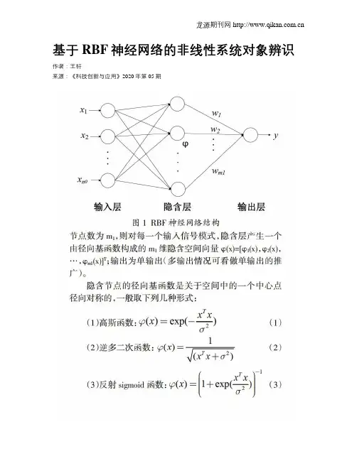
基于RBF神经网络的非线性系统对象辨识作者:王轩来源:《科技创新与应用》2020年第05期摘; 要:被控对象数学模型的精确建立是控制理论研究和发展的重要基础,但在实际工况中的控制系统多为复杂的非线性系统,因此高精度的非线性系统辨识技术显得至关重要。
RBF 神经网络具有对任意非线性函数逼近的能力,于是设计将RBF神经网络技术运用到系统辨识中,并通过Matlab仿真基于RBF神经网络对给定复杂非线性系统的辨识。
仿真结果表明在对于复杂非线性系统的辨识上,基于RBF神经网络的系统辨识法是准确可行的。
关键词:系统辨识;RBF神经网络;非线性系统;仿真中图分类号:TP273 文献标识码:A 文章编号:2095-2945(2020)05-0031-03Abstract: The establishment of accurate mathematical model of the controlled object is an important basis for the research and development of control theory, however, most of the control systems in actual working conditions are complex non-linear systems, therefore, high-precision non-linear system identification technology is very important. The RBF neural network has the ability to approximate non-linear functions, so the RBF neural network is designed to be used in system identification, and the given complex non-linear system is identified based on the neural network through Matlab simulation. Simulation results show that system identification based on RBF neural network is accurate and feasible for the identification of complex non-linear system.Keywords: system identification; RBF neural network; non-linear system; simulation系统辨识作为可以建立被控对象精确数学模型的学科是控制理论发展和应用的前提和基础。
1, neural network information processing mathematical processNeural network information processing can be used to illustrate the mathematical process, this process can be divided into two phases; the implementation phase and learning phase. The following note to the network before the two phases.1. Implementation phaseImplementation stage is the neural network to process the input information and generates the corresponding output process. In the implementation phase, the network structure and weights of the connection is already established and will not change. Then there is:X i (t +1) = f i [u i (t +1)]Where: X i is the pre-order neurons in the output;W ij is the first i of neurons and pre-j neurons synapse weightsθ i: i neurons is the first threshold;i-f i is the neuron activation function;I X i is the output neurons.2. Learning phaseNeural network learning phase is from the sound stage; this time, the learning network according to certain rule changes synaptic weights W ij,in order to enable end fixed measure function E is minimized. General access:E = (T i, X i) (1-9)Where, T i is the teacher signal;X i is the neuron output.Learning formula can be expressed as the following mathematical expression:Where: Ψ is a nonlinear function;η ij is the weight rate of change;n is the number of iterations during learning.For the gradient learning algorithm, you can use the following specific formula:Neural networks of information processing in general need to learn and implementation phases and combined to achieve a reasonable process. Neural network learning is to obtain information on the adaptability of information, or information of the characteristics; and neural network implementation process of information is characteristic of information retrieval or classification process.Learning and neural network implementation is indispensable to the two treatment and function. Neural network behavior and the role of various effective are two key processes by which to achieve.Through the study phase, can be a pair neural network training mode is particularly sensitive information, or have some characteristics of dynamic systems. Through the implementation phase, you can use neural networks to identify the information model or feature.In intelligent control, using neural network as controller, then the neural network learning is to learn the characteristics of controlled object, so that neural network can adapt to the input-output relationship between the controlled object; Thus, in implementation, neural network will be able to learn the knowledge of an object to achieve just the right control.Second, back-propagation BP modelNeural network learning is one of the most important and most impressive features. In neural network development process, learning algorithm has a very important position. At present, people put forward neural network model and learning algorithm are appropriate. So, sometimes people do not go to pray on the model and algorithm are strict definition or distinction. Some models can have a variety of algorithms. However, some algorithms may be used for a variety of models. However, sometimes also known as the model algorithm.Since the 40's Hebb learning rule has been proposed, people have proposed a variety of learning algorithms. Among them, in 1986, proposed by Rumelhart and other back-propagation method, that is, BP (error BackPropagation) method most widely affected. Even today, BP control algorithm is still the most important application of the most effective algorithm.1.2.1 Neural network learning mechanisms and institutionsIn the neural network, the model provided on the external environment to learn the training samples, and to store this model is called sensor; ability to adapt to external environment, can automatically extract the external environmental characteristics, is called cognitive device .Neural Networks in the study, generally divided into a study of two teachers and not teachers. Sensor signal by a teacher to learn, and cognitive devicesare used to learn without teacher signals. Such as BP neural network in the main network, Hopfield network, ART network and Kohonen network; BP network and Hopfield network is necessary for teachers to learn the signal can be; and ART network and Kohonen network signals do not need teachers to learn. The so-called teacher signal, that is, learning in neural network model of sample provided by an external signal.First, the learning structure of sensorPerceptron learning is the most typical neural network learning.At present, the control application is a multilayer feedforward network, which is a sensor model, learning algorithm is BP method, it is a supervised learning algorithm.A teacher of the learning system can be expressed in Figure 1-7. This learning system is divided into three parts: input Ministry of Training Department of the Ministry and output.Input received from outside the Department of input samples X, conducted by the Training Department to adjust the network weights W, and then the Department of the output from the output. Zai this process, the desired output signal can be used as teacher signal input, by the teacher signal and the actual output Jinxingbijiao, produce the Wucha right to Kongzhixiugai系数W.Learning organization structure can be expressed as shown in Figure 1-8.In the figure, X l, X 2, ..., X n, is the input sample signals, W 1, W 2, ..., W n are weights. Input sample signal X i can take discrete values "0" or "1." Input sample signa ls weights role in the u produces the output ΣW i X i, that is:u = ΣW i X i = W 1 X 1 + W 2 X 2 + ... + W n X nThen the desired output signal Y (t) and u compare the resulting error signal e. Body weight that is adjusted according to the error e to the power factor of the learning system be modified, modify the direction of the error e should be made smaller, and constantly go on, so that the error e is zero, then the actual output value of u and the desired output value Y ( t) exactly the same, then the end of the learning process.Neural network learning generally require repeated training, error tends gradually to zero, and finally reaches zero. Then the output will be consistent with expectations. neural network learning is the consumption of a certain period, some of the learning process to be repeated many times, even up to 10 000 secondary. The reason is that neural network weights W have a lot of weight W 1, W 2 ,---- W n; that is, more than one parameter to modify the system. Adjusting the system parameters must be time-consuming consumption. At present, the neural network to improve the learning speed and reduce thenumber of repeat learn the importance of research topic is real-time control of the key issues.Second, Perceptron learning algorithmSensor is a single-layer neural network computing unit, from the linear elements and the threshold component composition. Sensor shown in Figure 1-9.Figure 1-9 Sensor structureThe mathematical model of sensor:Where: f [.] Is a step function, and thereθ is the threshold.The greatest effect sensor is able to enter the sample classificationThat is, when the sensor output to 1, the input samples as A; output is -1, the input sample as B class. From the sensor can see the classification boundaries are:Only two components in the input sample X1, X2, then a classification boundary conditions:ThatW 1 X 1 + W 2 X 2-θ = 0 (1-17)Can also be written asThen the classification as shown in solid 1-10.Perceptron learning algorithm aims to find appropriate weights w = (w1.w2, ..., Wn), the system for a particular sample x = (xt, x2, ..., xn) Bear generate expectations d. When x is classified as category A, the expected value of d = 1; X to B class, d =- 1. To facilitate the description perceptron learningalgorithm, the threshold θ and w in the human factor, while the corresponding increase in the sample x is also a component of x n +1.So that:W n +1 =- θ, X n +1 = 1 (1-19)The sensor output can be expressed as:Perceptron learning algorithm as follows:1. Set initial value of the weights wOn the weights w = (W 1. W 2, ..., W n, W n +1) of the various components of the zero set of a small random value, but W n +1 =-G. And recorded as W l (0), W 2 (0), ..., W n (0), while there Wn +1 (0) =- θ. Where W i (t) as the time from i-tEnter the weight coefficient, i = 1,2, ..., n. W n +1 (t) for the time t when the threshold.2. Enter the same as the X = (X 1, X 2, ..., X n +1) and its expected output d. Desired output value d in samples of different classes are not the same time value. If x is A class, then take d = 1, if x is B, then take -1. The desired output signal d that is, the teacher.3. Calculate the actual output value of Y4. According to the actual output error e requeste = d-Y (t) (1-21)5. With error e to modify the weightsi = 1,2, ..., n, n +1 (1-22)Where, η is called the weight change rate, 0 <η ≤ 1In equation (1-22) in, η the value can not be too much. If a value too large will affect the w i (t) stability; the value can not be too small, too small will make W i (t) the process of deriving the convergence rate is too slow.When the actual output and expected the same d are:W i (t +1) = W i (t)6. Go to point 2, has been implementing to all the samples were stable. From the above equation (1-14) known, sensor is actually a classifier, it is this classification and the corresponding binary logic. Therefore, the sensor can be used to implement logic functions. Sensor to achieve the following logic function on the situation of some description.Example: Using sensors to achieve the logic function X 1 VX 2 of the true value:To X1VX2 = 1 for the A class to X1VX2 = 0 for the B category, there are equationsThat is:From (1-24) are:W 1≥θ, W 2≥θSo that W 1 = 1, W 2 = 2Have: θ ≤ 1Take θ = 0.5There are: X1 + X2-0.5 = 0, the classification shown in Figure 1-11.Figure 1-11 Logic Function X 1 VX 2 classification1.2.2 Gradient Neural Network LearningDevice from the flu, such as the learning algorithm known, the purpose of study is on changes in the network weights, so that the network model for the input samples can be correctly classified. When the study ended, that is when the neural network correctly classified, the weight coefficient is clearly reflected in similar samples of the input common mode characteristics. In other words, weight is stored in the input mode. As the power factor is theexisting decentralized, so there is a natural neural network distributed storage features.Sensor in front of the transfer function is a step function, so it can be used as a classifier. The previous section about the Perceptron learning algorithm because of its transfer function is simple and limitations.Perceptron learning algorithm is quite simple, and when the function to ensure convergence are linearly separable. But it is also problematic: that function is not linearly separable, then seek no results; Also, can not be extended to the general feed-forward network.In order to overcome the problems, so people put forward an alternative algorithm - gradient algorithm (that is, LMS method).In order to achieve gradient algorithm, so the neurons can be differential excitation function to function, such as Sigmoid function, Asymmetric Sigmoid function f (X) = 1 / (1 + e-x), Symmetric Sigmoid function f (X) = (1-e-x) / (1 + e-x); instead of type (1-13) of the step function.For a given sample set X i (i = 1,2,, n), gradient method seeks to find weights W *, so f [W *. X i] and the desired output Yi as close as possible.Set error e using the following formula, said:Where, Y i = f 〔W *· X i] is the corresponding sample X i s i real-time output I-Y i is the corresponding sample X i of the desired output.For the smallest error e, can first obtain the gradient of e:Of which:So that U k = W. X k, there are:That is:Finally, the negative gradient direction changes according to the weight coefficient W, amend the rules:Can also be written as:In the last type (1-30), type (1-31) in, μ is the weight change rate, the situation is different depending on different values, usually take between 0-1 decimal. Obviously, the gradient method than the original perceptron learning algorithm into a big step. The key lies in two things:1. Neuron transfer function using a continuous s-type function, rather than the step function;2. Changes on the weight coefficient used to control the error of gradient, rather than to control the error. dynamic characteristics can be better, that enhance its convergence process.But the gradient method for the actual study, the feeling is still too slow; Therefore, this algorithm is still not ideal.1.2.3 BP algorithm back-propagation learningBack-propagation algorithm, also known as BP. Because of this algorithm is essentially a mathematical model of neural network, so, sometimes referred to as BP model.BP algorithm is to solve the multilayer feedforward neural network weights optimization of their argument; Therefore, BP algorithm is also usually impliesthat the topology of neural network is a multilayer no feedback to the network. . Sometimes also called non-feedback neural networks using the BP model.Here, not too hard to distinguish between arguments and the relevant algorithms and models of both similarities and differences. Perceptron learning algorithm is a single-layer network learning algorithm. In the multi-layer network. It can only change the final weights. Therefore, the perceptron learning algorithm can not be used for multi-layer neural network learning. In 1986, Rumelhart proposed back propagation learning algorithm, that is, BP (backpropagation) algorithm. This algorithm can be in each layer, to amend the Weights and therefore suitable for multi-network learning. BP algorithm is the most widely used learning algorithm of neural network is one of the most useful in the control of the learning algorithm.1, BP algorithm theoryBP algorithm is used for feed-forward multi-layer network learning algorithm It contains input and output layer and input and output layers in the middle layer. The middle layer has single or multi-layer, because they have no direct contact with the outside world, it is also known as the hidden layer. In the hidden layer neurons, also known as hidden units. Although the hidden layer and the outside world are not connected. However, their status will affect therelationship between input and output. It is also said to change the hidden layer weights, you can change the multi-layer neural network performance.M with a layer of neural network and the input layer plus a sample of X; set the first layer of i k input neurons is expressed as the sum of U i k, the output X i k; k-1 layer from the first j months neuron to i-k layer neurons coefficient W ij the weight each neuron excitation function f, then the relationship between various variables related to mathematics can be expressed as the following:X i k = f (U i k)Back-propagation algorithm is divided into two parts, namely, forward propagation and back propagation. The work of these two processes are summarized below.1. Forward propagationInput samples from the input layer after layer of a layer of hidden units for processing, after the adoption of all the hidden layer, then transmitted to the output layer; in the process of layer processing, the state of neurons in each layer under a layer of nerve only element of state influence. In the output layer to the current output and expected output compare, if the current output is not equal to expected output, then enter the back-propagation process.2. Back-propagationReverse propagation, the error signal being transmitted by the original return path back, and each hidden layer neuron weights all be modified to look towards the smallest error signal.Second, BP algorithm is a mathematical expressionBP algorithm is essentially the problem to obtain the minimum error function. This algorithm uses linear programming in the steepest descent method, according to the negative gradient of error function changes the direction of weights.To illustrate the BP algorithm, first define the error function e. Get the desired output and the square of the difference between actual output and the error function, there are:Where: Y i is the expected output units; it is here used as teacher signals;X i m is the actual output; because the first m layer is output layer.As the BP algorithm by error function e of the negative gradient direction changes the weight coefficient, it changes the weight coefficient W ij the amount Aw ij, and eWhere: η is learning rate, that step.Clearly, according to the principles of BP algorithm, seeking ae / aW ij the most critical. The following requirements ae / aW ij; haveAsWhere: η is learning rate, that step, and generally the number between 0-1. Can see from above, d i k the actual algorithm is still significant given the end of the formula, the following requirements d i k formula.To facilitate derivation, taking f is continuous. And generally the non-linear continuous function, such as Sigmoid function. When taking a non-symmetrical Sigmoid function f, are:Have: f '(U i k) = f' (U i k) (1-f (U i k))= X i k (1-X i k) (1-45)Consider equation (1-43) in the partial differential ae / aX i k, there are two cases to be considered:If k = m, is the output layer, then there is Y i is the expected output, it is constant. From (1-34) haveThus d i m = X i m (1-X i m) (X i m-Y i)2. If k <m, then the layer is hidden layer. Then it should be considered on the floor effect, it has:From (1-41), the known include:From (1-33), the known are:Can see from the above process: multi-layer network training method is to add a sample of the input layer, and spread under the former rules:X i k = f (U i k)Keep one level to the output layer transfer, the final output in the output layer can be X i m.The Xim and compare the expected output Yi. If the two ranges, the resulting error signal eNumber of samples by repeated training, while gradually reducing the error on the right direction factor is corrected to achieve the eventual elimination of error. From the above formula can also be aware that if the network layer is higher, the use of a considerable amount of computation, slow convergence speed.To speed up the convergence rate, generally considered the last of the weight coefficient, and to amend it as the basis of this one, a modified formula:W here: η is the learning rate that step, η = 0.1-0.4 or soɑ constant for the correction weights, taking around 0.7-0.9.In the above formula (1-53) also known as the generalized Delta rule. For there is no hidden layer neural network, it is desirableWhere:, Y i is the desired output;X j is the actual output of output layer;X i for the input layer of input.This is obviously a very simple case, equation (1-55), also known as a simple Delta rule.In practice, only the generalized Delta rule type (1-53) or type (1-54) makes sense. Simple Delta rule type (1-55) only useful on the theoretical derivation. 3, BP algorithm stepsIn the back-propagation algorithm is applied to feed-forward multi-layer network, with the number of Sigmoid as excited face when the network can use the following steps recursively weights W ij strike. Note that for each floor there are n neurons, when, that is, i = 1,2, ..., n; j = 1,2, ..., n. For the first i-k layer neurons, there are n-weights W i1, W i2, ..., W in, another to take over - a W in +1for that threshold θ i; and the input sample X When taking x = (X 1, X 2, ..., X n, 1).Algorithm implementation steps are as follows:1. On the initial set weights W ij.On the weights W ij layers a smaller non-zero set of random numbers, but W i, n +1 =- θ.2. Enter a sample X = (x l, x 2, ..., x n, 1), and the corresponding desired output Y = (Y 1, Y 2, ..., Y n).3. Calculate the output levelsI-level for the first k output neurons X i k, are:X i k = f (U i k)4. Demand levels of learning error d i kFor the output layer has k = m, thered i m = X i m (1-X i m) (X i m-Y i)For the other layers, there5. Correction weights Wij and threshold θ Using equation (1-53) when:Using equation (1-54) when:Of which:6. When the weights obtained after the various levels, can determine whether a given quality indicators to meet the requirements. If you meet the requirements, then the algorithm end; If you do not meet the requirements, then return to (3) implementation.This learning process, for any given sample X p = (X p1, X p2, ... X pn, 1) and the desired output Y p = (Y p1, Y p2, ..., Y pn) have implemented until All input and output to meet the requirement.。
122自动化控制Automatic Control电子技术与软件工程Electronic Technology & Software Engineering1 概述过程控制常常遇到大惯性与纯滞后、多变量与耦合且对象模型时变不确定系统,控制系统结构和参数需要依靠经验和现场调试来确定。
PID 控制使用可靠、参数整定方便,成为过程控制常用的控制规律。
PID 控制三个控制参数其整定是控制系统设计的核心,往往参数整定完成后,整定好参数并不具有自适应能力,因生产环境发生改变,参数又需要重新整定。
利用神经网络多输入多输出以适应多变量与耦合、神经网络模型辨识以适应对象模型时变不确定性监测,使得控制具有良好在线自学习和自适应能力,可以很好发挥PID 比例、积分、微分控制优势。
2 系统设计2.1 总体设计设被控对象为:y(k)=g s [y(k-1),y(k-2),…,y(k-n),u(k-1),u(k-2),…u(k-m)]n>m (1)式(1)中被控对象的非线性特性g s (•)未知,需要神经网络辨基于神经网络系统辨识PID 控制的设计与仿真李建新(广州工商学院工学院 广东省广州市 528138)识器在线辨识以确定被控系统的模型。
PID 控制要取得较好的控制效果,关键在于调整好比例、积分和微分三种控制作用的关系。
在常规PID 控制器中,这种关系只能是简单的线性组合,因此难以适应复杂系统或复杂环境下的控制性能要求。
摘 要:本文为了实现生产过程有效控制,将神经网络、模型辨识和PID 控制技术结合,研究神经网络及系统辨识PID 控制。
该控制利用BP 神经网络学习技术实现PID 参数在线调整,同时采用BP 神经网络对被控对象在线辨识。
所设计的算法通过MATLEB 进行大量数据仿真,结果表明该控制实现了传统的PID控制算法无法适应的要求和对所开发的目标机良好移植性。
关键词:PID 控制;BP 神经网络;模型辨识;参数整定;权值调整图1:基于神经网络系统辨识PID 控制系统结构提高分类器的分类速度,达到了优化的目的。
神经网络的基本知识点总结一、神经元神经元是组成神经网络的最基本单元,它模拟了生物神经元的功能。
神经元接收来自其他神经元的输入信号,并进行加权求和,然后通过激活函数处理得到输出。
神经元的输入可以来自其他神经元或外部输入,它通过一个权重与输入信号相乘并求和,在加上偏置项后,经过激活函数处理得到输出。
二、神经网络结构神经网络可以分为多层,一般包括输入层、隐藏层和输出层。
输入层负责接收外部输入的信息,隐藏层负责提取特征,输出层负责输出最终的结果。
每一层都由多个神经元组成,神经元之间的连接由权重表示,每个神经元都有一个对应的偏置项。
通过调整权重和偏置项,神经网络可以学习并适应不同的模式和规律。
三、神经网络训练神经网络的训练通常是指通过反向传播算法来调整网络中每个神经元的权重和偏置项,使得网络的输出尽可能接近真实值。
神经网络的训练过程可以分为前向传播和反向传播两个阶段。
在前向传播过程中,输入数据通过神经网络的每一层,并得到最终的输出。
在反向传播过程中,通过计算损失函数的梯度,然后根据梯度下降算法调整网络中的权重和偏置项,最小化损失函数。
四、常见的激活函数激活函数负责对神经元的输出进行非线性变换,常见的激活函数有Sigmoid函数、Tanh函数、ReLU函数和Leaky ReLU函数等。
Sigmoid函数将输入限制在[0,1]之间,Tanh函数将输入限制在[-1,1]之间,ReLU函数在输入大于0时输出等于输入,小于0时输出为0,Leaky ReLU函数在输入小于0时有一个小的斜率。
选择合适的激活函数可以使神经网络更快地收敛,并且提高网络的非线性拟合能力。
五、常见的优化器优化器负责更新神经网络中每个神经元的权重和偏置项,常见的优化器有梯度下降法、随机梯度下降法、Mini-batch梯度下降法、动量法、Adam优化器等。
这些优化器通过不同的方式更新参数,以最小化损失函数并提高神经网络的性能。
六、常见的神经网络模型1、全连接神经网络(Fully Connected Neural Network):每个神经元与下一层的每个神经元都有连接,是最基础的神经网络结构。
神经网络模式识别法介绍神经网络模式识别法的基本原理是借鉴生物神经元的工作原理,通过构建多层的人工神经元网络,实现对复杂模式的学习和识别。
神经网络由输入层、隐藏层和输出层构成。
其中,输入层负责接收外界的输入模式,隐藏层是中间处理层,用来提取和转换输入模式的特征信息,输出层则是输出识别结果。
在神经网络模式识别方法中,关键的步骤有以下几个:1.数据预处理:首先需要对输入数据进行预处理,包括数据归一化、降噪和特征提取等。
这样可以使得神经网络更好地处理数据。
2.网络结构设计:根据实际问题的特点和要求,设计合适的神经网络结构。
可以选择不同的激活函数、网络层数、隐藏层神经元的数量等参数。
3.网络训练:利用已有的训练数据对神经网络进行训练。
训练过程中,通过反向传播算法来调整网络的权值和阈值,不断优化网络的性能。
4.网络测试:使用独立的测试数据对训练好的网络进行测试,评估其识别的准确性和性能。
可以通过计算准确率、召回率、F1值等指标来评估模型的效果。
神经网络模式识别方法有多种应用,如图像识别、语音识别、手写体识别等。
在图像识别领域,神经网络模式识别方法可以通过对图像的像素进行处理,提取图像的纹理、形状和颜色等特征,从而实现图像的自动识别。
在语音识别领域,神经网络模式识别方法可以通过对语音信号进行处理,提取声音特征,将语音信号转化为文本。
与其他模式识别方法相比,神经网络模式识别方法具有以下优点:1.具有自学习能力:神经网络可以通过反馈调整权值和阈值,不断优化自身的性能,从而实现模式识别的自学习和自适应。
2.并行性能好:神经网络中的神经元可以并行进行计算,能够快速处理大规模数据,提高了模式识别的效率。
3.对噪声鲁棒性好:神经网络能够通过反馈调整来适应输入数据中存在的噪声和不确定性,增强了模式识别的鲁棒性。
4.适应性好:神经网络模式识别方法适用于非线性问题和高维数据,能够处理复杂的模式识别任务。
尽管神经网络模式识别方法具有以上的优点,但也存在一些挑战和限制。
基于神经网络的非线性系统辨识随着人工智能技术的不断发展,神经网络技术成为人工智能领域中一个重要的研究方向。
神经网络具有自主学习、自适应和非线性等特点,因此在实际应用中有很大潜力。
本文将介绍神经网络在非线性系统辨识中的应用。
一、什么是非线性系统辨识?非线性系统辨识是指对一些非线性系统进行建模与识别,通过参数估计找到最佳的系统模型以进行预测分析和控制。
在许多实际应用中,非线性系统是比较常见的,因此非线性系统辨识技术的研究和应用具有重要的意义。
二、神经网络在非线性系统辨识中的应用神经网络在非线性系统辨识中具有很好的应用效果。
其主要原因是神经网络具有强大的非线性建模和逼近能力。
常用的神经网络模型包括前馈神经网络、递归神经网络和卷积神经网络等。
下面主要介绍前馈神经网络在非线性系统辨识中的应用。
1. 神经网络模型建立前馈神经网络由输入层、隐含层和输出层组成。
在非线性系统辨识中,输入层由外部输入量组成,隐含层用于提取输入量之间的非线性关系,输出层则用于输出系统的状态变量或输出变量。
模型建立的关键是隐含层神经元的个数和激活函数的选取。
2. 系统建模在非线性系统的建模过程中,需要将输出变量与输入变量之间的非线性关系进行建立。
可以使用最小二乘法、最小均方误差法等方法,对神经网络进行训练和学习,在一定的误差范围内拟合系统模型。
此外,也可以使用遗传算法、粒子群算法等优化算法来寻找最优的神经网络参数。
3. 系统预测和控制在系统建模和参数估计后,神经网络可以用于非线性系统的预测和控制。
在预测过程中,将系统的状态量输入前馈神经网络中,通过输出层的计算得到系统的输出量。
在控制过程中,将前馈神经网络与控制器相结合,在控制对象输出量和期望值不同时,自动调节控制器参数的值来实现系统的控制。
三、神经网络在非线性系统辨识中的优势和挑战与传统的线性系统模型相比,神经网络模型可以更好地描述非线性系统,并且可以用于对于非线性系统的建模和控制。
Script identification in the wild via discriminative convolutionalneural networkBaoguang Shi,Xiang Bai n,Cong YaoSchool of Electronic Information and Communications,Huazhong University of Science and Technology,Wuhan430074,Chinaa r t i c l e i n f oArticle history:Received25May2015Received in revised form23October2015Accepted10November2015Available online1December2015Keywords:Script identificationConvolutional neural networkMid-level representationDiscriminative clusteringDataseta b s t r a c tScript identification facilitates many important applications in document/video analysis.This paperinvestigates a relatively new problem:identifying scripts in natural images.The basic idea is combiningdeep features and mid-level representations into a globally trainable deep model.Specifically,a set ofdeep feature maps isfirstly extracted by a pre-trained CNN model from the input images,where the localdeep features are densely collected.Then,discriminative clustering is performed to learn a set of dis-criminative patterns based on such local features.A mid-level representation is obtained by encoding thelocal features based on the learned discriminative patterns(codebook).Finally,the mid-level repre-sentations and the deep features are jointly optimized in a deep network.Benefiting from such afine-grained classification strategy,the optimized deep model,termed Discriminative Convolutional NeuralNetwork(DisCNN),is capable of effectively revealing the subtle differences among the scripts difficult tobe distinguished,e.g.Chinese and Japanese.In addition,a large scale dataset containing16,291in-the-wild text images in13scripts,namely SIW-13,is created for evaluation.Our method is not limited toidentifying text images,and performs effectively on video and document scripts as well,not requiringany preprocess like binarization,segmentation or hand-crafted features.The experimental comparisonson the datasets including SIW-13,CVSI-2015and Multi-Script consistently demonstrate DisCNN a state-of-the-art approach for script identification.&2015Elsevier Ltd.All rights reserved.1.IntroductionScript identification is one of the key components in OpticalCharacter Recognition(OCR),which has received much attentionfrom the document analysis community,especially when the databeing processed is in multi-script or multi-language form.Due tothe rapidly increasing amount of multimedia data,especially thosecaptured and stored by mobile terminals,how to recognize textcontent in natural scenes has become an active and important taskin thefields of pattern recognition,computer vision and multi-media[15,16,25,26,47,49,59,23,57,38,8,41].Different from theprevious approaches which have been mainly designed for docu-ment images[48,19,20]or videos[40,58],this work focuses onidentifying the language/script types of texts in natural images(inthe wild),at word or text line level.This problem has seldom beenfully studied before.As texts in natural scenes often carry rich,high level semantics,there exist many efforts in scene text loca-lization and recognition[37,9,59,54–56,44].Script identification inthe wild is an inevitable preprocessing of a scene textunderstanding system under multi-lingual scenarios[5,6,22],potentially useful in many applications such as scene under-standing[32],product image search[17],mobile phone naviga-tion,film caption recognition[11],and machine translation[4,50].Given an input text image,the task of script identification is toclassify it into one of the pre-defined script categories(English,Chinese,Greek,etc.).Naturally,this problem can be cast as animage classification problem,which has been extensively studied.However,script identification in scene text images remains achallenging task,and has its characteristics that are quite differentfrom document/video script identification,or general image clas-sification,mainly due to the following reasons:1.In natural scenes,texts exhibit larger variations than they do indocuments or videos.They are often written/printed on outdoorsigns and advertisements,in some artistic styles.Often,thereexist large variations in their fonts,colors,and layout shapes.2.The quality of text images will affect the identification accuracy.As scene texts are often captured under uncontrolled environ-ments,the difficulties in identification may be caused by severalfactors such as low resolutions,noises,and illumination chan-ges.Document/video analysis techniques such as binarizationand component analysis tend to be unreliable.Contents lists available at ScienceDirectjournal homepage:/locate/prPattern Recognition/10.1016/j.patcog.2015.11.0050031-3203/&2015Elsevier Ltd.All rightsreserved.n Corresponding author.E-mail addresses:shibaoguang@(B.Shi),xbai@(X.Bai),yaocong2010@(C.Yao).Pattern Recognition52(2016)448–4583.Some scripts/languages have relatively minor differences,e.g.Greek,English and Russian.As illustrated in Fig.1,these scripts share a subset of characters that have exactly the same shapes.Distinguishing them relies on special characters or character components,and is afine-grained classification problem.4.Text images have arbitrary aspect ratios,since text strings havearbitrarily lengths,ruling out some image classification meth-ods that only operate onfixed-size inputs.Recently,CNN has achieved great success in image classifica-tion tasks[27],due to its strong capacity and invariance to translation and distortions.To handle the complex foregrounds and backgrounds in scene text images,we choose to adopt deep features learned by CNN as the basic representation.In our method,a deep feature hierarchy,which is a set of feature maps,is extracted from the input images through a pretrained CNN[29]. The hierarchy carries rich and multi-scale representations of the images.The differences among some certain scripts are subtle or even tiny,thus a holistic representation would not work well.Typical image classification algorithms,such as the conventional CNN[27] and the Single-Layer Networks(SLN)[10],usually describe images in a holistic style without explicit emphasis on discriminative patches that play an important role in distinguishing some script categories(e.g.English and Greek).Therefore,to explicitly capture fine-grained features of scripts,we extracted a set of common patterns,termed as discriminative patterns(the image patches containing the representative strokes or components)from script images via discriminative clustering[45].Such common patterns represented by deep features can be treated as a codebook for encoding the dense deep features into a feature vector,providing a mid-level representation of an input script image.A pooling strategy inspired by the Spatial Pyramid Pooling[18,28],called horizontal pooling,is adopted in the mid-level representation process.This strategy enables our method to capture topological structure of texts,and naturally handles input images of arbitrary aspect ratios.To maximize the discriminatory power of the mid-level representations,we put the above two modules,namely the convolutional layers for extracting deep feature hierarchy and the discriminative encoder for extracting the mid-level representa-tions,into a single deep network for joint optimization with the back-propagation algorithm[30].The globalfine-tuning process optimizes both the deep features and the mid-level representa-tion,effectively integrating the global features(deep feature maps)andfine-grained features(discriminative patterns)for script identification.This paper is a continuation and extension of our previous work[43].In[43]we have proposed Multi-stage Spatially sensitive Pooling Network(MSPN)and a10-classes dataset called SIW-10 for the in-the-wild script identification pared with[43], this paper describes text images via discriminative mid-level representation,instead of the global horizontal pooling on con-volutional feature maps.Discriminative patches corresponding to special characters or components are explicitly discovered and used for building the mid-level representation.In addition,this paper proposes a larger and more challenging dataset with13 script classes.In summary,the contributions of the paper are as follows:(1)A discriminative mid-level representation built on deep features is presented for script identification tasks,in contrast to other methods that rely on texture,edge or connected component analysis.(2)We show that the mid-level representation and the deep feature extraction can be incorporated in a deep model,and get jointly optimized.(3)The proposed method is not limited to script identification in the wild,applicable to video and document script identification as well.The highly competitive performances are consistently achieved on such three kinds of script bench-marks.(4)Compared to the previously collected SIW-10,a larger and more challenging dataset SIW-13is created and released.The remainder of this paper is organized as follows:In Section2 related work in script identification and image classification is reviewed and compared.In Section3the proposed method is described in detail.In Section4we introduce the SIW-13dataset. The experimental evaluation,comparisons with other methods,and some discussions are presented in Section5.We conclude our paper in Section6.2.Related work2.1.Script identificationPrevious works on script identification mainly focus on texts in documents[48,20,7,24]and videos[40,58].Script identification can be done at document page level,paragraph or text-block level, text-line level or word/character level.An extensive and detailed survey has been made by Ghosh et al.in[14].Text images can be classified by their textures.Some previous works conduct texture analysis to extract some kind of holistic appearance descriptors of the input image.Tan[48]proposes to extract rotation invariant texture features for identifying docu-ment scripts.In[7],several texture features,including gray-level co-occurrence matrix features,Gabor energy features,and wavelet energy features,are tested.Joshi et al.[24]present a generalized framework to identify scripts at paragraph and text-block levels. Their method is based on texture analysis and a two-level hier-archical classification scheme.Phan et al.[40]propose to identify text-line level video scripts using edge-based features.The fea-tures are extracted from the smoothness and cursiveness of the upper and lower lines in each of thefive equally sized horizontal zones of the text lines.In[58],Zhao et al.present features that are based on Spatial Gradient-Features at text block level,building features from horizontal and vertical gradients.Manthalkar et al.[34]propose rotation and scale invariant texture features,using discrete wavelet packet transform.Texture analysis,although widely adopted,may be insufficient to identify scripts,especially when distinguishing scripts that share common characters.Instead of texture analysis,our approach uses a discriminative mid-level representation,whichEnglish GreekRussianFig.1.Illustration of the script identification task and its challenges:Both fore-grounds and backgrounds exhibit large variations and high level of noise.Mean-while,characters“A”,“B”and“E”appear in all the three scripts.Identifying themrelies on special patterns that are unique to certain scripts.B.Shi et al./Pattern Recognition52(2016)448–458449tends to be more effective in distinguishing between scripts that have subtle appearance difference.Some other approaches analyze texts via their shapes and structures.In[46],a method based on structure analysis is intro-duced.Different topological and structural features,including number of loops,water reservoir concept features,headline fea-tures and profile features,are combined.Hochberg et al.[20] discover a set of templates by clustering“textual symbols”,which are connected components extracted from training scripts.Test scripts are then compared with these templates tofind their best matching ponent based methods,however,are usually limited to binarized document scripts,since in video or natural scenes images it is hard to achieve ideal binarization.Our approach does not rely on any binarization or segmentation techniques.It is applicable to not only documents,but also a much wider range of scenarios including scene texts and video texts. 2.2.Image classificationNaturally,script identification can be cast as an image classifi-cation problem.The Bag-of-Words(BoW)framework[31]is a technique that is widely adopted in image classification problems. In BoW,local descriptors such as SIFT[33],HOG[12]or simply raw pixel patches[10]are extracted from images,and encoded by some coding methods such as the locality-constrained linear coding(LLC[52])or the triangle activation[10].Recent research on image classification and other visual tasks has seen a leap forward, thanks to the wide application of deep convolutional neural net-works(CNNs[29]).CNN is deep neural network equipped with convolutional layers.It learns the feature representation from raw pixels,and can be trained in an end-to-end manner by the back-propagation algorithm[30].CNN,however,is not specially designed for the script identification task.It cannot handle images with arbitrary aspect ratios,and it does not put emphasis on dis-criminative local patches,which may be crucial for distinguishing scripts that have subtle differences.3.Methodology3.1.OverviewGiven a cropped text image I,which may contain a word or sentence written horizontally,we predict its script class c A f1;…;C g.As illustrated in Fig.2,the training process is divided into two stages.In thefirst stage,we build a discriminative mid-level representation,from the deep feature hierarchies (Section 3.2)extracted by a pretrained CNN,using the dis-criminative clustering method(Section3.3).The result is a dis-criminative codebook that contains a set of linear classifiers.We use the codebook to build the mid-level representation(Section 3.4).In the second stage(Section 3.5),we model the feature extraction,mid-level representation andfinal classification into one neural network.The network is initialized by transferring parameters(weights)learned in thefirst stage.We train the net-work using back-propagation.Consequently,parameters of all modules getfine-tuned together.3.2.Deep feature Hierarchy extractionThe input image isfirstly represented by a convolutional fea-ture hierarchy f h l g L l¼1,where each h l is a set of feature maps with the same size,and L is the number of levels in the hierarchy.The feature hierarchy is extracted by a pretrained CNN,which is dis-cussed in Section5.1.The input text image I isfirstly resized to a fixed height(32pixels throughout our experiments),keeping their aspect ratios.Thefirst level of the feature hierarchy h1is extracted by performing convolution and max-pooling with convolutional filters f k1i;j gi;jand biases f b1jgj,resulting in feature mapsh1¼f h1j gj¼1;…;n1.Each feature map h j1is computed by:h1j¼mpσX n0i¼1I i n k1i;jþb1j!!:ð1ÞHere,I i represents the i-th channel of the input image.n0is the number of image channels.The star operator n indicates the2-D convolution operation.σðÁÞis the squashing function which is an element-wise non-linearity.In our implementation,we use the element-wise thresholding function maxð0;xÞ,also known as the ReLU[36].mp is the max-pooling function,which downsamples feature maps by taking the maximum values on downsampling subregions.The remaining levels of the feature hierarchy are extracted recursively,by performing convolution and max-pooling on the feature maps from the preceding hierarchy level:h lj¼mpσXn lÀ1i¼1h i n k l i;jþb l j!!:ð2ÞHere,l is the level index in the hierarchy.Since image down-sampling is applied,the sizes of the feature maps decrease with l.The extracted feature hierarchy f h l g L l¼1provides dense local descriptors on the input image.At each level l,the feature mapsh l¼f h l k g n lk¼1are extracted by applying convolutional kernels densely on either the input image I or the feature maps h lÀ1fromFig.2.Illustration of the training process of the proposed approach.B.Shi et al./Pattern Recognition52(2016)448–458450the preceding level.A pixel on the feature map h lk ½i ;j ,where i and j are the row and column indices,respectively,is determined by a corresponding subregion on the input image,also known as the receptive field [21].As illustrated in Fig.3,the concatenation of thepixel values across all feature maps x l ½i ;j ¼½h l 1½i ;j ;…;h ln l ½i ;j T is taken as the local descriptor of that subregion.Since down-sampling is applied,the size of the subregion increases with level l .Therefore,the extracted feature hierarchy provides dense local descriptors at several different scales.The feature hierarchy is rich and invariant to various image distortions,making the representation robust to various distor-tions and variations in natural scenes.In addition,convolutional features are learned from data,thus domain-speci fic and poten-tially stronger than general hand-crafted features such as SIFT [33]and HOG [12].3.3.Discriminative patch discoveryAs we have discussed in Section 1,one challenging aspect of the script identi fication task is that some scripts share a subset of characters that have the same visual shapes,making it dif ficult to distinguish them via some holistic representations,such as texture features.The visual differences between these scripts can be observed only via a few local regions,or discriminative patches [45],which may correspond to special characters or special char-acter components.These patches are observed in certain scripts,and are strong evidence for identifying the script type.For example,characters “Λ”and “Σ”are distinctive to Greek.If the input image contains any of them,it is likely to be Greek.In our approach,we discover these discriminative patches from local patches extracted from the training images.The patches are described by deep features.As we have described in Section 3.2,the feature hierarchies provide dense local descriptors.Therefore we simply compute all feature hierarchies and extract dense local descriptors from them.To discover the discriminative visual pat-terns from the set of local patches,we adopt the method proposed by Singh et al.in [45],which is a discriminative clustering method for discovering patches that are both representative and discriminative.Given the set of local patches described by deep features,the discriminative clustering algorithm outputs a discriminative codebook,which contains a set of linear classi fiers.The clustering is performed separately on each class c and on each feature level l .For each class c ,a set of local descriptors X l c is extracted from the feature hierarchies,taken as the discovery set [45].Another set,the natural set ,contains local descriptors from the remaining classes.The discriminative clustering algorithm is performed on the twosets,resulting in a multi-class linear classi fier f w l c ;b lc g .The finaldiscriminative codebook is built by concatenating the classi fierweights from all classes,i.e.K l ¼ðW l ;b lÞ.Detailed descriptions are listed in Algorithm 1.Algorithm 1.The discriminative clustering process.1:Input:Local descriptors f x l i g i ;l ¼1…L2:Output:Discriminative clusters f K l g l ¼1…L 3:for feature level l ¼1to L do 4:for class c ¼1to C do 5:Discovery set D l c ¼f x l :x l A X l c g 6:Natural set N l c ¼f x l :x l =2X l c g7:w l c ;b lc ¼discriminative_clustering ðD l c ;N l c Þ8:end for9:W l ;b l¼concat c ðf W l c gÞ;concat c ðf b lc g10:K l ¼ðW l ;b lÞ11:end for12:Output f K l g l ¼1…LFig.4shows some examples of the discriminative patches discovered from feature level 4(the last convolutional layer).Among the patches,we can observe special characters or text components that are distinctive to certain scripts.The dis-criminative clustering algorithm automatically chooses the num-ber of clusters.In our experiments,it results in a codebook with about 1500classi fiers on each feature level.3.4.Mid-level representationTo obtain the mid-level representation,we firstly encode the feature maps in the hierarchy with the learned discriminative codebook,then horizontally pool the encoding results into a fixed-length vector.Assuming that the feature maps have the shape n Âw Âh ,as mentioned,from the maps we can densely extract w Âh local descriptors,each of n dimensions.Each local descriptor,say x ½i ;j where i ,j are the location on the map,is encoded with the discriminative codebook that has k entries (i.e.k linear clas-si fiers),resulting in a k -dimensional vector z ½i ;j :z l ½i ;j ¼max ð0;W l x l ½i ;j þb lÞ:ð3ÞHere,the encoded vector is the non-negative response of all theclassi fiers in the codebook.W l x l ½i ;j þb lis the responses of all k classi fiers.A positive response indicates the presence of certain discriminative patterns,and is kept,while negative responses are suppressed by setting them to zero.To describe the whole image from the encoding results,we adopt a horizontal pooling scheme,inspired by the spatial pyramid pooling (SPP [18]).Texts in real world are mostly horizontally written.The horizontal positions of individual characters are less meaningful for identifying the script type.Their vertical positions of the text components such as strokes,on the other hand,are useful since they capture structure of the characters.To make the representation invariant to the horizontal positions of local descriptors,while maintaining the topological structure on the vertical direction,we propose to take the maximum response along each row of the feature maps,i.e.take max j z l ½i ;j .The maximum responses are concatenated as a long vector,which captures the topological structure of characters,and are invariant to the character positions or orderings.We call the module for extracting this mid-level representation discriminative encoder .Itis parameterized by the codebook weights,i.e.W l and b l.Fig.3.Locations on the feature maps and their corresponding receptive fields on the input image.The concatenation of the values on that location across all feature maps form the descriptor of the receptive field,consequently dense local descriptors at different scales can be extracted from the feature hierarchy.B.Shi et al./Pattern Recognition 52(2016)448–4584513.5.Global fine-tuningFine-tuning is the process of optimizing the parameters of several algorithm components in a joint ually fine-tuning is carried out in a neural network structure,where gradients on layer parameters are calculated with the back-propagation algorithm [30].In global fine-tuning,we aim to optimize the parameters (weights)of all components involved,including the convolutional feature extractor,the discriminative codebook,and the final clas-si fier.To achieve this,we model the components into network layers,forming an end-to-end network that maps the input image into the final predicted labels,and apply the back-propagation algorithm to optimize it.Discriminative encoding layer:We model the discriminative encoding process as a network layer.According to Eq.(3),the linear transform W x þb is firstly applied to all locations on the feature maps,equivalent to the linear transform on the map level.Then,a threshold function max ð0;x Þis applied,equivalent to the ReLU nonlinearity.Therefore,we model the layer as the sequential combination of a linear layer that is parameterized by codebook weights W ,b ,and an ReLU layer.We call this layer the dis-criminative encoding (DE)layer.Horizontal pooling layer:The horizontal pooling process can be readily modeled as the horizontal pooling layer,which is inserted after each DE layer.Multi-level encoding and pooling:The feature maps on different hierarchy levels describe the input image on different scales andabstraction levels.We believe that they are complementary with each other for classi fication.Therefore,we construct a network topology that utilizes multiple feature hierarchy levels.The topology is illustrated in Fig.5.We insert discriminative encoding þhorizontal pooling layers after multiple convolutional layers,and concatenate their outputs into a long vector,which is fed to the final classi fication layers.The resulted network is initialized by the weights learned in previous procedures.Speci fically,the convolutional layers are initialized by the weights in the convolutional feature extractor.The weights in the discriminative layers are transferred from the discriminative codebook.The weights in the classi fication layers are randomly initialized.The network is fine-tuned with the back-propagation algorithm.4.The SIW-13datasetThere exist several public datasets that consist of texts in the wild,for instance,ICDAR 2011[42],SVT [53]and IIIT 5K-Word [35].However,these datasets are primarily used for scene text detec-tion and recognition tasks.Besides,these datasets are dominated by English or other Latin-based scripts.Other scripts,such as Arabic,Cambodian and Tibetan,are rarely seen in these datasets.In the area of script identi fication,there exist several datasets [20,40,58].However,the datasets proposed in these works mainly focus on texts extracted from documents orvideos.Fig.4.Examples of discriminative patches discovered from the training data.Each row shows a discovered cluster,which corresponds to a special character that is unique to a certain script,e.g.row 1for Greek,row 6for Japanese and row 8for Korean.B.Shi et al./Pattern Recognition 52(2016)448–458452In this paper,we propose a dataset 1for script identi fication in wild scenes.The dataset contains a large number of cropped text images taken from natural scene images.As illustrated in Fig.6,the dataset contains text images from 13different scripts:Arabic,Cambodian,Chinese,English,Greek,Hebrew,Japanese,Kannada,Korean,Mongolian,Russian,Thai and Tibetan.We call this dataset the Script Identi fication in the Wild 13Classes (SIW-13)dataset.For collecting the dataset,we first harvest a collection of street view images from the Google Street View [1]and manually label the bounding boxes of text regions,as shown in Fig.7.Text images are then cropped out,and recti fied by being rotated to the hor-izontal orientation.For each script,about 600–1000street view images are collected,and about 1000–2000text images are cropped out.Totally,the dataset contains 16,291text images.For benchmarking script identi fication algorithms,we split the dataset into the training and testing sets.The testing set contains all together 6500samples,with 500samples for each class.The remaining 9791samples are used for training.Table 1lists the detailed statistics of the dataset.Some examples of the collected dataset are shown in Fig.6.Since images are collected in natural scenes images,texts in the images exhibit large variations in fonts,color,layout and writing styles.The backgrounds are sometimes cluttered and complex.In some cases,text images are blurred or affected by lighting conditions or cameraposes.These factors make our dataset realistic,and much more challenging than datasets that are collected from document or videos.The SIW-13dataset is extended from our previously pro-posed SIW-10[43].Three new scripts,namely Cambodian,Kannada and Mongolian,are added.Also,we revise the remaining script classes by removing images that are either too noisy or corrupted,and by adding some new images to these classes.5.ExperimentsIn this section,we evaluate the performance of the proposed DiscCNN on three tasks,namely script identi fication in the wild,in videos and in documents,and compare it with other widely used image classi fication or script identi fication methods,including the conventional CNN,the SLN [10]and the LBP.5.1.Implementation detailsWe use the same network structure throughout our experi-ments,with the exception of the discriminative encoding layers,whose structures and initial parameters are determined auto-matically by the discriminative patch discovery process.As illu-strated in Figs.2and 5,we use feature levels 2,3,and 4for patch discovery and discriminative encoding.In the discovery step,the number of local descriptors can be large,especially when the feature maps have large size.For this reason,we use only a part of the extracted local descriptors for patch discovery on feature levels 2and 3.For the first stage in our approach,the convolutional layers are pretrained by a conventional CNN whose structure is speci fied in Table 2.The network is jointly optimized by stochastic gradient descent (SGD)with the learning rate set to 10À3,the momentum set to 0.9and the batch size set to 128.The network uses the dropout strategy in the last hidden layer with a dropout rate 0.5during training.The learning rate is multiplied by 0.1when the validation error stops decreasing for enough number of iterations.The network optimization process terminates until the learning rate reaches 10À6.The proposed approach is implemented using C þþand Python.On a machine with the Intel Core i5-2320CPU (3.00GHz),8GB RAM and a NVIDIA GTX 660GPU,the feature hierarchy extraction and discriminative clustering takes about 4h.The GPU accelerated fine-tuning process takes about 8h to reach con-vergence.Running on a GPU device,the testing process takes less than 20ms for each image,and consumes less than 50MBRAM.Chinese Cambodian Arabic English Greek Hebrew Japanese Kannada Korean Mongolian RussianThai TibetanFig.6.Examples of cropped text images in the SIW-13dataset.Fig.5.The structure and parameters of the deep network model.The network consists of four convolutional layers (conv1to conv4),three discriminative encoding layers (DE-1,DE-2and DE-3)and two fully connected layers (fc1and fc2).Discriminative encoding layers are inserted after convolutional layers conv2,conv3and conv4.Their outputs are concatenated as a long vector,and passed to the fully connected layers.(For interpretation of the references to color in this figure,the reader is referred to the web version of this paper.)1The dataset can be downloaded at /$xbai/mspnProjectPage/.It is available for academic use only.B.Shi et al./Pattern Recognition 52(2016)448–458453。