patran分析实例 螺栓分析
- 格式:pdf
- 大小:7.22 MB
- 文档页数:15

文章主题:patran螺栓预紧力的参考点在机械设计和工程中,螺栓预紧力是一个至关重要的参数。
它决定了螺栓的紧固效果和工作性能,直接关系到机械设备的安全和可靠性。
而patran螺栓预紧力作为一个常用的预紧力工具,在工程领域中应用广泛。
1. patran螺栓预紧力的概念与原理patran螺栓预紧力是一种通过计算机辅助设计软件来模拟和计算螺栓预紧力的方法。
其原理是利用有限元分析方法,对螺栓和螺母的连接进行模拟,通过施加预紧加载,得出螺栓的预紧力大小。
这种方法可以直观地呈现出螺栓连接的受力状态,对于工程师来说非常直观和便捷。
2. patran螺栓预紧力的应用领域在实际的工程设计中,patran螺栓预紧力可广泛应用于各种机械设备、车辆和建筑工程中。
汽车发动机的螺栓连接、高铁轨道的螺栓紧固、建筑结构的螺栓连接等。
通过对螺栓预紧力的计算和分析,可以有效地提高设备的安全性和可靠性,减少故障的发生。
3. patran螺栓预紧力的计算方法通常,计算patran螺栓预紧力需要考虑一系列因素,包括螺栓的材料、螺纹形状、预紧加载力的施加方式等。
在实际工程中,可以通过调整这些参数,来优化螺栓的预紧效果。
并且,通过有限元分析软件的模拟,可以得到更加准确和可靠的预紧力数值。
4. 个人观点和理解从个人的角度来看,patran螺栓预紧力的应用对于机械工程设计和制造来说无疑是一项十分重要的技术。
它不仅可以提高产品的质量和性能,也能够减少因螺栓脱落或故障而造成的安全事故。
在未来,我相信随着计算机辅助设计技术的不断发展,patran螺栓预紧力的应用将会更加普及和成熟。
总结回顾通过本文的讨论,我们对patran螺栓预紧力有了更加深入和全面的了解。
我们从概念与原理、应用领域、计算方法及个人观点等方面进行了探讨,以期帮助读者更加深入地理解和应用这一技术。
patran螺栓预紧力的参考点是机械工程设计和制造中的一个重要技术,它为我们提供了一种模拟和计算螺栓预紧力的便捷方法,对于提高产品性能和安全性具有重要意义。
实验:装配的模态有限元分析
一. 问题描述
探究结合面的参数对装配体的模态有限元分析影响因素,做如下实验设计两块简单的平板,用两螺栓连接,模拟机床部件之间结合面的形式。
具体参数如下
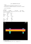
1. 建立如下图所示的装配图
尺寸描述如下:
板长360mm 宽84MM 上板厚10mm 下板后 30mm
为了说明分析情况与实际相符,螺栓分布不对称距离中心分别为 140mm 和100mm 装配体分为上下两个板结构
上板为板1 下板为板2
材料铸铁铸铁
弹性模量 145e9 145e9
伯松比0.25 0.25
密度7.3G/CM 7.3G/CM
螺栓螺帽
材料碳钢碳钢
弹性模量 200E9 200E9
伯松比0.3 0.3
密度7.9 7.9
2 .对装配体划分网格
为了计算准确有考虑计算机性能,选择二次单元,solid 8node 183 单元
划分完效果图如下:
可以看到这是自由网格划分的情况,用的是四面体单元 精度不如二次六面体单元
四面体单元和三角形单元混合的使用
下面进行求解自由模态
选择分析类型和设置约束之后求解得到结果
其中设置的是以板2下面约束所有自由度。
自由状态的模态分析结果。
与下面的约束方法做比较。
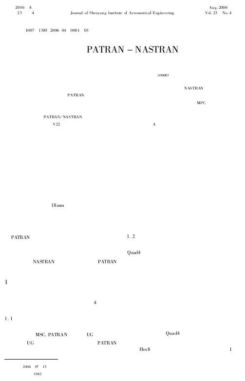
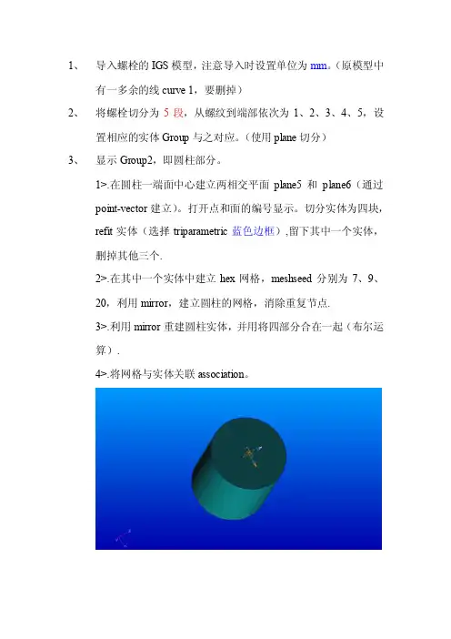
1、导入螺栓的IGS模型,注意导入时设置单位为mm。
(原模型中有一多余的线curve 1,要删掉)2、将螺栓切分为5段,从螺纹到端部依次为1、2、3、4、5,设置相应的实体Group与之对应。
(使用plane切分)3、显示Group2,即圆柱部分。
1>.在圆柱一端面中心建立两相交平面plane5和plane6(通过point-vector建立)。
打开点和面的编号显示。
切分实体为四块,refit实体(选择triparametric蓝色边框),留下其中一个实体,删掉其他三个.2>.在其中一个实体中建立hex网格,meshseed分别为7、9、20,利用mirror,建立圆柱的网格,消除重复节点.3>.利用mirror重建圆柱实体,并用将四部分合在一起(布尔运算).4>.将网格与实体关联association。
4、显示Group3,即圆柱与螺栓端部的倒角部分。
建模方法与圆柱部分相同,建好网格后,将Group2和Group3的网格合并在一起。
5、显示Group4,即螺栓端部的正六棱柱。
1>.将底部平面用plane5和plane6分为四部分。
不要删掉六棱柱的底面,即相当于重建图的8个面。
只取其中的四分之一,删掉其余的面。
2>.用两点的连线将不规则的面打断为两个曲面四边形,这样就可以画出quad网格。
在边上种下meshseed(要与圆台部分协调),绘制quad网格。
3>.两次mirror后+消除重复节点后建立底面网格。
list这些网格,创建Group记为surface。
删掉新建的平面。
4>.将网格沿棱柱高度方向sweep,注意拉伸长度为6.35485mm。
将网格与实体关联association。
5>.显示Group2、3、4,消除重复节点。
6、显示Group1,即螺纹部分。
1>.利用plane5和plane6分割上端面为四个面。
不要删掉原面,新建四个面,与第5步一样,建立与圆柱协调的网格。
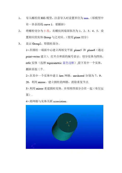
某沿海双体客船系泊锚泊支撑结构设计作者:王轩黄涣青来源:《广东造船》2020年第02期摘要:本文介紹了中国船级社《规范》对系泊锚泊设备支撑结构的设计和计算方法,并以某沿海双体客船为实例,对该船首尾系泊锚泊设备支撑结构的设计进行阐述。
基于Patran/Nastran有限元软件,建立包含舷墙和锚机基座的船体有限元模型,对各系泊锚泊设备进行受力分析,校核其支撑结构强度。
计算结果表明,该船系泊锚泊支撑结构满足《规范》的相关强度要求,可为同类船舶系泊锚泊支撑结构设计提供参考。
根据计算结果,对设计方案提出建议和注意事项。
关键词:系泊锚泊;支撑结构;强度计算中图分类号:U663.7 文献标识码:AAbstract: This paper introduces the design and calculation method of supporting structure of mooring and anchoring equipment in the rules of China Classification Society (CCS), and takes a coastal passenger catamaran as a design example to describe the design method of fore and aft mooring equipment supporting structure. The finite element model of hull including bulwark structure and windlass foundation is established based on Patran / Nastran software, and the force analysis and strength check are carried out for the mooring and anchoring equipment and its supporting structure. The results show that the supporting structure of the ship meets the relevant strength requirement of the CCS’s rules and can provide reference for the design of mooring and anchoring supporting structure of similar ships. Some suggestions and matters needing attentions are put forward according to the calculation results.Key words: Mooring and anchoring; Supporting structure; Strength calculation1 前言船舶系泊锚泊设备在工作时,会受到较大的集中载荷。

1 概述螺栓是机载设备设计中常用的联接件之一。
其具有结构简单,拆装方便,调整容易等优点,被广泛应用于航空、航天、汽车以及各种工程结构之中。
在航空机载环境下,由于振动冲击的影响,设备往往产生较大的过载,对作为紧固件的螺栓带来强度高要求。
螺栓是否满足强度要求,关系到机载设备的稳定性和安全性。
传统力学的解析方法对螺栓进行强度校核,主要是运用力的分解和平移原理,解力学平衡方程,借助理论和经验公式,理想化和公式化。
没有考虑到连接部件整体性、力的传递途径、部件的局部细节(如应力集中、应力分布)等等。
通过有限元法,整体建模,局部细化,可以弥补传统力学解析的缺陷。
用有限元分析软件MSC.Patran/MSC.Nastran提供的特殊单元来模拟螺栓连接,过程更方便,计算更精确,结果更可靠。
因此,有限元在螺栓强度校核中的应用越来越广泛。
2 有限元模型的建立对于螺栓的模拟,有多种模拟方法,如多点约束单元法和梁元法等。
多点约束单元法(MPC)即采用特殊单元RBE2来模拟螺栓连接。
在螺栓连接处,设置其中一节点为从节点(Dependent),另外一个节点为主节点(Independent)。
主从节点之间位移约束关系使得从节点跟随主节点位移变化。
比例因子选为1,使从节点和主节点位移变化协调一致,从而模拟实际工作状态下,螺栓对法兰的连接紧固作用。
梁元法模拟即采用两节点梁单元Beam,其能承受拉伸、剪切、扭转。
通过参数设置,使梁元与螺栓几何属性一致。
本文分别用算例来说明这两种方法的可行性。
2.1 几何模型如图1所示组合装配体,底部约束。
两圆筒连接法兰通过8颗螺栓固定。
端面受联合载荷作用。
图1 三维几何模型2.2 单元及网格抽取圆筒壁中性面建模,采用四节点壳元(shell),设置壳元厚度等于实际壁厚。
法兰处的过渡圆弧处网格节点设置密一些,其它可以相对稀疏。
在法兰上下两节点之间建立多点约束单元(RBE2,算例1,图3)或梁元(Beam, 算例2,图4)来模拟该位置处的螺栓连接。
1、导入螺栓的IGS模型,注意导入时设置单位为mm。
(原模型中有一多余的线curve 1,要删掉)2、将螺栓切分为5段,从螺纹到端部依次为1、2、3、4、5,设置相应的实体Group与之对应。
(使用plane切分)3、显示Group2,即圆柱部分。
1>.在圆柱一端面中心建立两相交平面plane5和plane6(通过point-vector建立)。
打开点和面的编号显示。
切分实体为四块,refit实体(选择triparametric蓝色边框),留下其中一个实体,删掉其他三个.2>.在其中一个实体中建立hex网格,meshseed分别为7、9、20,利用mirror,建立圆柱的网格,消除重复节点.3>.利用mirror重建圆柱实体,并用将四部分合在一起(布尔运算).4>.将网格与实体关联association。
4、显示Group3,即圆柱与螺栓端部的倒角部分。
建模方法与圆柱部分相同,建好网格后,将Group2和Group3的网格合并在一起。
5、显示Group4,即螺栓端部的正六棱柱。
1>.将底部平面用plane5和plane6分为四部分。
不要删掉六棱柱的底面,即相当于重建图的8个面。
只取其中的四分之一,删掉其余的面。
2>.用两点的连线将不规则的面打断为两个曲面四边形,这样就可以画出quad网格。
在边上种下meshseed(要与圆台部分协调),绘制quad网格。
3>.两次mirror后+消除重复节点后建立底面网格。
list这些网格,创建Group记为surface。
删掉新建的平面。
4>.将网格沿棱柱高度方向sweep,注意拉伸长度为6.35485mm。
将网格与实体关联association。
5>.显示Group2、3、4,消除重复节点。
6、显示Group1,即螺纹部分。
1>.利用plane5和plane6分割上端面为四个面。
不要删掉原面,新建四个面,与第5步一样,建立与圆柱协调的网格。

结构刚度对机翼连接件连接螺栓载荷分配的影响王启明【摘要】机翼连接件是静不定结构,载荷的传递很难用传统的静定结构进行受力分析.利用PATRAN/NASTRAN软件对机翼连接件进行有限元建模,对连接件存在的螺栓连接和端面接触问题,进行了合理的有限元模拟,重点分析了翼型结构特性对螺栓载荷分配的影响.为比较结构刚度变化对螺栓载荷的影响,分别调整连接件局部刚度和结构整体刚度,通过有限元分析,得出了螺栓载荷分配随结构刚度的变化规律,对机翼连接结构设计具有一定的参考价值.【期刊名称】《机械制造与自动化》【年(卷),期】2016(045)001【总页数】4页(P50-53)【关键词】机翼;连接件;有限元模型;结构刚度;载荷【作者】王启明【作者单位】南京航空航天大学航空宇航学院,江苏南京210016【正文语种】中文【中图分类】V214.1+1;TP391.9机翼连接件是飞机结构中典型的连接构件,其结构特征决定了传力特性和载荷分配关系,是结构设计的重要环节之一。
连接件在使用中始终处于交变载荷作用,受力情况复杂,容易产生应力集中和结构疲劳现象,机翼连接件很难用传统的静定结构传力路线分析方法来确定受力情况和危险部位[1]。
工程上通常通过建立有限元模型的方法来进行受力特征分析,确定螺栓载荷和危险部位。
目前对于机械连接多钉结构钉载分配方面的研究文献很多。
谢鸣九[2]研究了多排钉连接的各钉排的承载比例,发现钉排数越多,中间的钉排承载越小,多于4排钉的连接对降低最严重钉排承载比例的作用很小。
杨晓宇[3]研究了不同刚度板的连接,其钉载分配类似,但不再对称,载荷向刚度大的板一侧的螺栓上转移。
文献[4]用梁元与弹簧元模拟螺栓连接进行了比较,表明梁元和弹簧元都适于研究钉群载荷的分配,同时提出采用梁元加间隙元模拟螺栓与螺栓孔之间的挤压作用, 能够更准确地反映螺栓孔附近的应力场。
以往的大多数文献研究的是比较规则的板钉之间单钉或多钉的钉载分配,而对于实际工程结构机械连接研究较少。

双锥密封结构设计蒲弦【摘要】用MSC.Patran&Nastran有限元分析软件建立三维分析模型对某氨合成塔的双锥密封系统进行应力分析,阐述此类非线性接触分析的过程.【期刊名称】《化工设计》【年(卷),期】2013(023)002【总页数】4页(P26-29)【关键词】双锥环密封;有限元;接触分析【作者】蒲弦【作者单位】中国成达工程有限公司成都610041【正文语种】中文密封结构的设计是压力容器结构设计的重要部分。
通常的密封形式有强制密封,半自紧密封和自紧密封三种形式。
在低、中压压力容器中通常采用强制密封结构,如法兰连接结构,其特点是依靠上紧螺柱产生垫片预紧力,从而达到初始密封,当压力升高时,垫片能产生足够的回弹力而达到操作工况下的密封能力。
在高压容器的密封结构中,通常采用半自紧式密封,如双锥密封,透镜垫密封等,其原理类似于强制密封,在预紧时,通过螺柱的预紧达到垫片的预紧载荷形成初始密封,当操作工况下的压力上升时,由于螺柱呈拉伸趋势,从而使垫片产生的轴向回弹力有减小趋势,径向方向由于压力作用,产生向外扩展趋势并紧密贴合于密封面达到更好的密封;自紧式密封,通常用于超高压设备中,如楔形垫密封结构,随着压力的升高,密封面上的压紧力随之增大,密封更为可靠。
图1 双锥密封结构高压设备的密封结构设计中采用的双锥密封结构形式,是典型的半自紧式密封系统。
双锥密封系统主要由筒体端部、双锥环垫、非金属软垫或金属软垫、压紧盖、主螺柱、螺母组成,见图1。
按新修订的GB 150-2011标准,双锥密封可适用的温度范围0~400℃,压力为6.4MPa~35MPa,直径为400mm~3200mm。
相比GB150-98版,直径范围上限由2000mm变为3200mm,并对影响密封性能的径向间隙g值的调整为(0.1%~0.075%)D1。
对于0℃以下的操作工况可以参照标准进行设计。
常规设计时,双锥密封系统的设计主要分为双锥密封结构尺寸的设计和主螺柱的设计。
MSC的应用实例--螺栓建模MSC软件公司是计算机辅助工程(CAE)行业的最初领导者,是从“Nastran公司”成长成为真正的市场和技术的模拟软件的领先者,包括线性和非线性有限元分析(FEA),多体动力学,控制系统,以及许多其他应。
我们的产品能够准确,可靠地预测产品在未来现实世界中的表现,以帮助工程师可以设计更好,更创新的产品——快速和富有成本效率的。
使用MSC产品,企业能够消除缓慢而昂贵的物理测试,通过创建和测试“虚拟原型”,可以快速作出任何环境或条件下的性能评估,以实现持久的竞争优势。
Patran是世界上使用最广泛的有限元分析(FEA)预/后处理软件,能够提供实体建模,网格划分,以及为MSC Nastran,Marc, Abaqus, LS-DYNA, ANSYS,和Pam-Crash提供分析设置。
MSC Nastran的是世界上使用最广泛的有限元分析(FEA)求解器。
当涉及到模拟压力,动力,还是现实世界的震动以及复杂的系统时,MSC Nastran仍然是目前世界上最好的和最值得信赖的软件。
今天,有限元求解器是可靠和准确的,足以通过FAA和其他监管机构的认证,所以零件到复杂装配的制造商都选择了有限元求解器。
SimXpert是新一代计算机辅助工程(CAE)应用软件,应用在使用有限元和多体动力学(MBD)进行的建模和分析中。
与MSC的先进的多学科综合(MD)求解器技术相结合,SimXpert提供了一个有效的“终端到终端”的解决方案,该方案能够使您从进行计算机辅助设计(CAD)转为在一个易于使用的应用程序中进行分析报告。
Marc和Mentat相结合,为隐式非线性有限元分析提供完整的解决方案(预处理,解决和后处理)。
Marc 为接触,大压变和多物理饭呢西提供了最容易使用和最强大的能力,从而能够解决当今的静态和准静态非线性问题。
双剪多排螺栓连接螺栓孔接触域应力分布研究徐建薪;陈文俊;李顶河;贾宝慧【摘要】Based on the method of dealing with contact problem, a finite element analysis model of multiple bolt-jointed plate was established by MSC.Patran/Nastran software. The stress distribution around bolt-hole contact area was investigated. During analyzing variation of stress distribution in each row of bolt hole, the changes of the bolt-hole clearance and the roughness on the contact surface were mainly considered. It is found that bolt-hole clearance and friction coefficent have greater influences on stress distribution in the bolt -hole extruded surface, but these factors can not destroy the similarity of stress distribution in each row of bolts. In the process of modeling,the bolt wss defined as the flexible contact body. Considering the contact friction as well as elastic deformation between the bolt and aluminum plate,the results are more accurate and reliable than that of previous analysis model that bolts were defined as the rigid body.%基于接触问题的研究方法,利用由MSC.Patran/Nastran软件建立的多排双剪螺栓连接有限元模型,对螺栓-孔接触域上的应力分布进行了研究.研究过程中主要考虑在不同的间隙和接触面粗糙度下,各排螺栓的应力分布变化规律.研究发现间隙和粗糙度对孔受压面上的应力影响较大,但不能破坏各排螺栓孔应力分布规律的相似性.在建模过程中,将螺栓定义为可变性接触体,考虑了螺栓与铝板之间的接触摩擦以及相互间弹性变形,比以往的刚性体螺栓具有更高的准确性和可靠性.【期刊名称】《中国民航大学学报》【年(卷),期】2011(029)005【总页数】4页(P8-11)【关键词】螺栓连接;应力分布;接触应力;有限元法【作者】徐建薪;陈文俊;李顶河;贾宝慧【作者单位】中国民航大学航空工程学院,天津300300;中国民航大学航空工程学院,天津300300;中国民航大学航空工程学院,天津300300;中国民航大学航空工程学院,天津300300【正文语种】中文【中图分类】TB31;V229在航天、航空、交通等工程领域,螺栓连接是最常用的机械连接方式。
Patran实验报告飞行器制造083614 孙诚骁实验一:二维面受力本实验采用面单元,旨在说明平面薄板端点受力后的应力情况,采用面单元,isomesh的网格划分,平面端点处受到向下的8N的力,材料采用铝,弹性模量取10e6Von-mises屈服条件下的应力图,应力最大值出现在根部,打到2.25e4MPa实验二:梁单元受力本实验旨在说明1D单元网格划分和2D单元网格划分的受力分析在pratran中计算结果相同,以证明patran软件在这方面的正确性1.矩形截面端点加载采用面单元网格划分,isomesh、quad4;末端方形截面左上端点受到10N向下的力,根部固支;材料为铝。
计算结果为最大应力出现在根部,为356Mpa2.杆结构加载对比采用节点划分单元。
根部固支,受到10N向下的力,作用点在12,与末端11节点距离为0.75,采用铝材料。
计算结果为根部应力最大为360Mpa(L型杆末端加力)下图旨在证明力系简化的正确性,将上图中的力平移到11节点,力分成了作用在11节点的向下的10N的力和一个X方向大小为7.5Nm的扭矩。
分析结果与上图相同。
(等效载荷:直杆末端受力与弯矩)实验三:3D结构受力分析本实验采用3D实体建模,采用Tetmesh、tet10网格划分。
实体受到孔边集中力,模拟螺栓连接,底部三孔固支。
材料为铝。
(变形后与变形前对比)(von-mises应力分布图)(孔边应力图)实验四:平板受力采用自定义的单元网格划分,分为面单元和线单元,面单元和线单元规整排列。
材料为铝,受力为面压力。
(z方向变形图)(Von-mises应力图)。
锚机支撑结构局部强度两种直接计算方法对比王佚;张少雄;张华【摘要】In the direct strength assessment of the windlass's foundation and its supporting structures, two methods to apply the loadings are adopted, and the stress results are compared and analyzed.It can be concluded that both of the methods can be used to assess the local strength of the windlass's foundation and its supporting structures when the stress level is low, when the stress is close to the allowable stress, the method using MPC is recommended.%采用两种加载方式对某浮吊锚机基座及相关船体结构的局部强度进行直接计算,并对比分析两种方法所得的应力结果,结果表明,两种方法是应力结果差别较大,在应力水平较低时两种方法都可以用来计算校核基座及其支撑结构的局部强度;当应力水平接近许用应力时,建议采用MPC加载方式计算评估。
【期刊名称】《船海工程》【年(卷),期】2015(000)006【总页数】6页(P50-54,59)【关键词】锚机;局部强度;有限元;直接计算【作者】王佚;张少雄;张华【作者单位】武汉理工大学交通学院,武汉430063;武汉理工大学交通学院,武汉430063;中国船级社上海审图中心,上海200135【正文语种】中文【中图分类】U663.7随着船舶吨位不断增大,锚系泊力越来越大。
参数化建模的螺栓法兰连接刚度分析蒋国庆;李家文;唐国金【摘要】为分析几何参数对螺栓法兰连接刚度的影响,用 MSC.Patran 软件的二次开发工具 PCL(Patran Command Language)建立了螺栓法兰连接的参数化模型。
研究了螺栓法兰连接刚度随连接结构几何参数的变化规律并进行了灵敏度分析。
经分析可知,连接结构刚度对开孔位置比例参数最敏感,其次是上法兰厚度。
当上部段长度大于某一数值时,连接结构刚度对上部段长度参数不敏感,这一结论能为连接结构动力学简化建模提供一定理论参考。
%In order to analyze the effects of geometric parameters on the stiffness of bolted flange joint,a parameterized model of bolted flange joint was constructed by using PCL (Patran Command Language)on the platform of software MSC.Patran.The law of the stiffness of bolted flange joint with the change of geometric parameters was studied,and the sensitivity of geometric parameters was analyzed based on the parameterized model.The results show that theratio of the location of hole is the most sensitive factor to the stiffness of bolted flange joint,and the next one is thickness of upper flange.When the length of upper body is up to a const,the stiffness of bolted flange joint is insensitive to the length of upper body,and this conclusion can provide a reference to simplify the dynamic model of joint.【期刊名称】《国防科技大学学报》【年(卷),期】2014(000)006【总页数】5页(P180-184)【关键词】PCL;螺栓法兰连接;参数化;灵敏度【作者】蒋国庆;李家文;唐国金【作者单位】国防科技大学航天科学与工程学院,湖南长沙 410073;国防科技大学航天科学与工程学院,湖南长沙 410073;国防科技大学航天科学与工程学院,湖南长沙 410073【正文语种】中文【中图分类】V435螺栓法兰结构具有构造简单、可靠性高、可操作性好、使用维护简便[1]等特点,在工业结构中应用十分广泛。
MSC 软件公司: Patran 产品介绍产品介绍Patran 软件介绍集成的并行框架式有限元前后处理及分析仿真系统随着世界市场竞争的日趋激烈, 制造厂商们越来越清楚的意识到 CAE 在其产品设计制造过程中的重要地位;由于产品性能仿真所涉及学科的多样性和 CAD 系统间各具特色,迫切需要能够将多种CAE 仿真集成在一个易学易用、统一完整的平台上。
Patran正是从这一角度出发开发的有限元框架式平台,设计者可以方便地根据自己的需求进行多学科的工程分析和数据交换。
因此,Patran被广泛应用于航空、航天、汽车、船舶、铁道、机械、制造业、电子、建筑、土木、国防、生物力学、食品包装、教学研究等各个行业。
一. Patran 的主要特点◆符合CAE流程的用户界面◆极好的兼容性、开放性◆强大的客户化定制功能(PCL语言)◆CAD 模型的直接访问技术(DGA)◆高级面网格剖分功能,可在复杂的带有缺陷的曲面上快速生成高质量的面网格,并提供方便的用户可控性◆支持多种CAE求解器◆独特的复合材料建模工具LAMINATE MODELER◆支持疲劳分析建模◆独特的变量场技术◆不同硬件平台和操作系统下数据库兼容◆大模型快速图形操作航空发动机结构分析模型汽车发动机部件模型曲轴模型二. Patran 的主要功能1.用户界面和软件性能图形用户界面Patran友好的用户界面条理清晰, 符合CAE操作流程,最多不超过三级的菜单按"事件"激发, 使用户可随意接通任何分析任务。
丰富的电子表格工具, 如弹出或下拉式菜单与表格、滑动条、图形图标、按钮。
" 单击和拖动"及多功能屏汽车分析模型幕拾取选择等, 可用于输入和管理数据。
各类表格均使用普通的工程术语, 当需要时辅助表格或自动弹出或自动消失,整个界面直观易懂。
Patran对大模型的操作响应极快,包括网格剖分、图形优化、数据库优化、内存管理及屏幕刷新等,都能快速给出操作结果,这样将大大加快分析速度。
Suranaree J. Sci. Technol. 14(4):331-345Fatigue and Fracture Research Group, Department of Mechanical and Manufacturing Engineering,University of Putra Malaysia, 43400 Serdang, Selangor, Malaysia. E-mail: aidy@.my *Corresponding authorSIMULATION AND EXPERIMENTAL WORK OF SINGLE LAP BOLTED JOINT TESTED IN BENDINGAidy Ali *, Ting Wei Y ao, Nuraini Abdul Aziz, Muhammad Yunin Hassan and Barkawi SahariReceived: Jun 13, 2007; Revised: Nov 29, 2007; Accepted: Nov 30, 2007AbstractThis paper presents the simulation and experiment work on the prediction of stress analysis in a single lap bolted joint under bending loads. A three-dimensional finite element model of a bolted joint has been developed using MSC Patran and MSC Nastran FEM commercial package. In the simulation, different methods in modelling the contact between the joint, which affects the efficiency of the models were detailed. Experimental work was then conducted to measure strains and deformations of the specimens for validation of the developed numerical model. A four-point bending load type of testing was used in both the simulation and experiment works. The results from both simulation and experiment were then compared and show good agreement. Several factors that potentially influenced the variation of the results were noted. Finally, critical areas were identified and confirmed with the stress distribution results from simulation.Keywords: Bolted joints, FEM, MSC Nastran, MSC PatranIntroductionA bolted joint is one of the joining techniques employed to hold two or more parts together to form an assembly in mechanical structures. One of the advantages of a bolted joint over other joint types, such as welded and riveted joints, is that they are capable of being dismantled.A bolted j oint is considered as an important element to be employed in civil, mechanical and aeronautic structures.The previous studies on the behaviour of a single lap bolted joint were mostly dedicated to tension load at the end of plate. An early studywas performed by Ireman (1998) in which a three-dimensional finite element model of bolted composite j oints was developed to determine the non-uniform stress distribution through the thickness of composite laminates in the vicinity of a bolt hole. The single lap bolted joint was loaded in tension. A similar study was carried out by McCarthy et al. (2005) where the effects of bolt-hole clearance on the mechanical behaviour of a bolted composite (graphite/epoxy) j oint were investigated. Furthermore,Ju et al. (2004) studied the nominal applied(a)Figure 1. (a) Geometry and (b) marking of SAE Grade 5 Hex bolt333 Suranaree J. Sci. Technol. V ol. 14 No. 4; October-December 2007Geometry ModellingIn simulation, the geometry scale factor is determined as 1,000 (millimeter). Generally, the unit used in MSC Patran modelling is listed in Table 3 below.The geometry of the model is based on two solid plates (170 × 74 × 9 mm), one support plate (40 × 74 × 9 mm), and a unit consisting of a bolt and a nut. The bolt hole, of radius 6.25mm, is edited in the upper and lower plate by Boolean method and the substrate. The diameter of the bolt shank is assumed to fully fit in the bolt hole. Figure 2 shows the geometry of the FEM model. As illustrated, the position of origin is pointed by the arrow; direction represents the length of the plate, y direction represents the width of the plate, and z direction represents the thickness of the plate.Table 1. Properties and dimension of the bolt and nutMaterial type Medium carbon steel,Quenched and tempered Modulus of elasticity, E200 GPaPoisson’s ratio, Å0.29Proof strength586 MPaMinimum tensile yield strength634 MPaMinimum tensile ultimate strength827 MPaNominal length, L38.1 mmNominal diameter, D12.3 mmHeight of bolt, H7.0 mmWidth across flat, F18.5 mmWidth across corners, C21.5 mmHeight of nut11.0 mmTable 2. Properties and dimension of the platesMaterial type Mild steelModulus of elasticity, E200 GPaPoisson’s ratio, Å0.29Thickness9.0 mmWidth74.0 mmTable 3. Unit and parameter used in MSC Patran ModellingParameter Unit (SI)Length m mForce NMass TonnesTime SecondStress MPa (N/mm2)Density Tonnes/mm334Simulation and Experimental work of Single Lap Bolted Joint Tested in BendingIn order to assist the analysis, the stresses at the regimes of interest were analysed as labelled in Figure 3. The stress distribution along the middle of surfaces of upper plate symmetry is taken from Profile (a) and Profile (b). Profile (c) and Profile (d) are designed to compare the stress distribution along the bolt hole in different locations. Profile (e) is taken along the middle of the bolt.Mesh GenerationThe element used on the bolt and plates is the same with SOLID type Tet10. The total elements in the model are 6,665 and the numbers of nodes are 11,954. The action of “Equivalent”is applied on the mesh of the model to delete the nodes which are duplicated between the surface contacts. Finally, the mesh was verified to test the failure of aspect ratio, edge angle, face skew, collapse, normal offset, tangent offset, Jacobian ratio and Jacobian zero. The verification summary (Figure 4) showed the number of failures the elements involved. Zero number of failures is desired to minimize error in the analysis process.A contact element was introduced through multi-point constraint (MPC). MPC is employed in the finite element model to solve the problem of the more detailed free body load in the overall model. MPC is A linear combination of displace-ment. Generally, one displacement is dependent on the remaining independent displacement (Brown, 1987). In this model, three types of MPC were introduced in different situation. The first MPC is created between the bolt and the two plates. The MPC type used is Rigid (fixed). A single point constraint is used to prevent rigid body motion. As shown in Figure 5, Node 10824 in the middle of the bolt shank was defined as an independent term and the nodes on the bolt hole of the plates are defined as dependent terms. The second MPC, RBE2 was employed on the overlap region between the upper plate and support plate as illustrated in Figure 6.Finally, the third MPC Explicit was used to define the contact condition between two plates. In this technique, the dependent term is on the edge of the lower plate while the inde-pendent terms are the nodes of the upper plate in the overlap region. The coefficient of friction is input and 6 degrees of freedom is selected. The value of coefficient of friction is assumed as 0.74 (Beardmore, 2007).Boundary ConditionIn this section, displacement is created to constrain the model from translating when a bending load is applied. The ideal displacement is applied in a line/curve to uniform the displace-ment distribution. The locations of displacement are 25 mm and 225 mm in x direction from the origin. However, in this model, the applicationFigure 2. Geometry modelling and position of originSuranaree J. Sci. Technol. V ol. 14 No. 4; October-December 2007335Figure 3. Profile (a) to (e) of interest in stress distributionFigure 4. Verification of meshFigure 5. Location and terms of MPC 1336Simulation and Experimental work of Single Lap Bolted Joint Tested in Bendingregion is determined by those nodes which are on the desired lines (Figure 7). These nodes are constrained by fixing the degrees of freedom; translations are in x, y, and z directions. LoadingsIn this step, two types of loads were considered which are the clamping force and bending force. The clamping force is applied by uniform pressure onto the overlap area between the bolt nut and the plates (Figure 8).A clamping force of 100 N is modelled by using a negative pressure value. The bending force is applied onto the upper plate by selecting those nodes which are close to the ideal location as shown in Figure 9. The load locations applied is 85 mm and 165 mm in direction x in origin. Experimental ProceduresThe experimental work was carried out in the Strength Laboratory at UPM to test four-point-bending on a single lap bolted joint. The results obtained in the experimental measurements are load-displacement and load-strain data. The experimental load-displacement curves wereFigure 6. MPC 2 between upper plate and support plateFigure 7. Boundary condition of the joint337 Suranaree J. Sci. Technol. V ol. 14 No. 4; October-December 2007obtained directly from the testing machine. Strains at selected points on the joint surface were measured while bending forces were controlled manually by the Instron Universal Testing Machine. The surface of the lower plate was strain-gauged in the axial direction. Figure 10 shows the position of the unidirec-tional strain gauge, which had a 5 mm gauge length. Axial strain in the plate is observed for every increment of 1 kN. The specimen and jigs were mounted on the universal testing machine as illustrated in Figure 11. The bending load was applied by the lower load cell vertically, while the top load cell was fixed. The application of the load was controlled manually to obtain the strains measurement for every increasing load level.Results and DiscussionJoint DeformationThe deformed shape of the finite element model is shown together with the actual defor-mation in Figure 12. The experimental load-deflection curves were found to be essentiallyFigure 8. Clamping force in uniform pressureFigure 9. Application of bending load338Simulation and Experimental work of Single Lap Bolted Joint Tested in BendingFigure 10. Strain-gauge (a) location (b) set upFigure 11. Experimental configurationAll dimensions in mm (a)(b)339 Suranaree J. Sci. Technol. V ol. 14 No. 4; October-December 2007linear up to and including 7 kN. Since the experi-mental specimen deformation becomes non-linear plastic behavior after 7 kN, the shape of the experimental and finite element model with applied load 7 kN is shown for comparison.It can be seen that the finite element model displays similar deformation shape to the experiment. From Figure 12(b), penetration of the master line (upper plate) into slave nodes (lower plate) shows the effect of contact between two deformable bodies. It is seen from Figure 12(a) and (b) that the agreement of the presence of a gap between the upper plate and lower plate due to the effect of the bending load is gener-ally good. The experimental load-displacement curves were found to be essentially linear untilan applied load of 7 kN, so the displacements of the experimental and finite element model were measured over this range. Figure 13 shows the calibration curves of load-displacement of the experimental and finite element model under elastic region of three tested samples.Progressive Stress Distribution at Different Load LevelIn this section, stress distribution of the joint is observed at different load levels to track the stress distribution in each parts of the joint as shown in Figure 14. This technique possesses accurate prediction of stress distri-bution. The applied load levels used in the analysis are 0 kN, 1 kN, 4 Kn, and 7 kN. The (a)(b)Figure 12. Joint deformation of (a) experimental specimen and (b) FEM model340Simulation and Experimental work of Single Lap Bolted Joint Tested in Bendingrelative magnitude of the stress distribution on the bolt head decreases with the increasing load level when compared with the stress on the plates. It can be observed that the bolt nut starts to loosen when bending force is applied. As expected, higher stress is distributed at the bending and constraint area as illustrated in Figure 15 when the specimen experienced 15 kN bending load. Non-symmetrical stress distribu-tion along the x-axis is due to the non-uniform mesh in the model.Stress Distribution of Interest RegimesStress distribution along a path is studied by developing several regimes of interest in order to assist the analysis. Profile (a) and Profile (b) given in Figure 16 show the compari-son of stress distribution on both surfaces of the upper plate. The purpose of mapping these profiles is to observe the tension and compres-sive stress of bending. Along the path of both profiles, the stress increases gradually to the edge of the bolt hole, no stress exists in the hole, and the stress decreases smoothly to the end of the plate. The upper and lower stress distributions observed were similar; these represent the maximum tension and maximum compressive stress having the same value as well as established in text books. The highest stress is found at the edge of the bolt hole which is caused by the combination of clamping force and bending force.In order to measure the stress distribu-tion along the bolt hole surface of both plates, Profile (c) and Profile (d) were developed. The stress in this section is the same as the stress in the bolt for no clearance between the hole and bolt. The paths of both profiles begin from the edge of the lower plate bolt hole along y axis. The results of the stresses distribution of these two profiles are shown in Figure 17. The trend of stress along the path shows that the maximum stress occurs between the contact of the upper and lower plates. This phenomenon is caused by the combination of contact stress, clamping force and bending force. Obvious differences between the stress of Profile (c) and Profile (d) can be seen. This occurs when heavier contact stress between the bolt shank and bolt hole occurs due to bending. Then again, higher stress at the edge of the bolt hole shows agree-ment with the clamping force between the bolt nut and plates.Finally, the stress distribution in the bolt is measured by observing Profile (e) as shown in Figure 18. It is interesting to note that theFigure 13. Comparison of load-displacement curve between the experiment and FEM model(a)(b)(c)(d)Figure 14.Progressive stress distribution at different load levels (a) 0 kN, (b) 1 kN, (c) 4 kN, and(d) 7 kNFigure 15. Deformation of specimen after 15 kN bending forceFigure 16. Comparison of Profile (a) and (b) stress distribution along the pathFigure 17. Comparison of Profile (c) and (d): stress distribution along the pathstress changes non-uniformly along the path and increases sharply at the end of the bolt head.This phenomenon is due to the bending force increasing the tension in the bolt head.In spite of the critical area occuring on the surface of upper plate of the single lap bolted joint as predicted, it is interesting to investigate the critical area of the bolt and nut, since it was the main component in the joint. From the simulation result, it was observed that the critical areas in terms of V on Mises stress, of the bolt and nut were between the clamping surfaces of the bolt head. The critical area of the FEM bolt-nut as well as the experimental specimen bolt is shown in Figure 20. The simulation shows that the bolts will experienced cracks and failures. On the other hand, the plate will experienced deformation due to the bolt pen-etration will loaded in bending. The joint strength of the bolted joint still relies on the strength of its bolts in both cases, when thetension and bending loads were applied.Figure 18. Profile (e) stress distribution along the pathFigure19.(a) Critical area in terms of Von Mises criterion in the joint (b) closer view of thecritical area (c) experimental specimen. (The arrows points to the critical area of the joint)(c)and Stanley, W.F. (2005). Three-dimen-sional finite element analysis of single-bolt, single-lap composite bolted joint:Part I – Model development and valida-tion. Composite Structure, 71(2):140-155. Su, R.K.L. and Siu, W.H. (2004). Nonlinear response of bolt groups under in-planeloading. Engineering Structures, 26(3):403-413.Unified Engineering. (2006). H ex head bolt makings. Aurora, IL. Available from: Inc./scitech/bolt/boltmarks.html. Accessed date: Apr 26,2007.。