Are employers discriminating with respect to weight- European Evidence using Quantile Regression

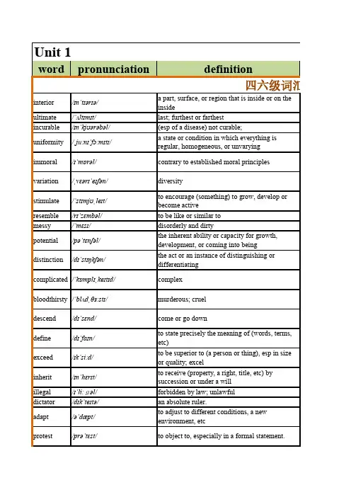
access/ˈæksɛs/the act of approaching or entering device/dɪˈvaɪs/ a machine or tool used for a specific taskclue/kluː/something that helps to solve a problem or unravel a mysteryliberalism/ˈlɪbərəˌlɪzəm/the state or quality of being liberal.chronology/krəˈnɒlədʒɪ/the science that deals with the determination of dates and the sequence of eventsgraphologist/græˈfɒlədʒɪst/a specialist in inferring character from handwritingretrospect/ˈrɛtrəʊˌspɛkt/the act of surveying things past genetic/dʒɪˈnɛtɪk/of or relating to genetics, genes portray/pɔːˈtreɪ/make a picture ofdisintegrate/dɪsˈɪntɪˌɡreɪt/to become reduced to components, fragments, or particlesgrilled/ɡrɪld/cooked on a grill or gridirongregarious/ɡrɪˈɡɛərɪəs/enjoying the company of othersravenous/ˈrævənəs/extremely hungryslither/ˈslɪðə/to move or walk with a sliding motion, as a snakesalvage/ˈsælvɪdʒ/the act of saving any goods or property in danger of damage or destructionape/eɪp/ a monkey inflammable/ɪnˈflæməbəl/liable to catch fire concentric/kənˈsɛntrɪk/having a common centreauditorium/ɔːdɪˈtɔːrɪəm/the area of a theater or concert hall where the audience sitsinscription/ɪnˈskrɪpʃən/something inscribed, esp words carved or engraved on a coin, tomb, etcinhale/ɪnˈheɪl/breathe intitan/ˈtaɪtən/ a person of great strength or sizeprenatal/priːˈneɪtəl/previous to birth or to giving birth四六级范围外词汇pounce/pouns/to spring or swoop with intent to seize someone or somethingbeverage/ˈbɛvərɪdʒ/any drink, usually other than watersourdough/ˈsaʊəˌdəʊ/(of bread) made with fermented dough used as a leaven生僻词For years, newspaper companies have been offering Web access free.The program detects the e-reader and automatically downloads new content to the device.They distract us mid-conversation and make us miss the critical clue in the mystery we're watching at the theater.Liberalism, above all, means emancipation—emancipation from one's fears, his inadequacies, from prejudice, from discrimination ... from poverty.The book also offers the first accurate and in-depth chronology of aturbulent journey from criminal to icon.They hire a graphologist and make us submit handwriting samples.However harmless they are in retrospect, they never fail to startle, always causing me to pause and look around.Law would bar insurers and employers from discriminating based ongenetic testing.The cruelest thing a man can do to a woman is to portray her as perfection.Before these images, all words disintegrate and fall lifeless into the ashes.They are typically served in the form of grilled or poached fillets.外词汇The problem was that her gregarious confidence vanished in social settings.Beware of false prophets, who come to you in sheep's clothing but inwardly are ravenous wolves.On campus-visit days, worries slither into the thoughts of the hosts.After a decade of poor planning, the space agency is hoping to salvage what it can.He was, however, convinced that the hairs were not of a bear or ape.The shock scattered its glowing contents through the car, and in an instant the highly inflammable woodwork was blazing.Bands of color in concentric circles are also a popular design.The auditorium, band room and choir room are off limits because they have been condemned.Cards are blank inside for your personal inscription.They will notice how air fills their lungs when they inhale and gets pushed out when they exhale.The soft drink titans are struggling for control of the market.Most cases are diagnosed after birth now, but if the blood test is widelyadopted it could become chiefly a prenatal event.We all know the power of waiting quietly for the right moment to pounce upon an opportunity.No longer a luxury item, the beverage has become a common sightworldwide.词With some rustic sourdough bread, it made a delicious appetizer for ourdinner.。

职业歧视英语作文英文回答：Occupational discrimination, also known as job discrimination, refers to the unfair treatment of an individual or group based on their protected characteristics, such as race, religion, gender, sexual orientation, disability, or age. This discrimination can manifest in various forms, including hiring, firing, promotion, compensation, benefits, and working conditions.There are various laws and regulations in place to prohibit occupational discrimination. In the United States, the Civil Rights Act of 1964, the Equal Employment Opportunity Act of 1972, and the Americans withDisabilities Act of 1990 are key pieces of legislation that protect individuals from workplace discrimination. These laws prohibit employers from discriminating against employees based on their protected characteristics and require them to provide reasonable accommodations foremployees with disabilities.In addition to legal protections, employers have a moral and ethical responsibility to prevent and address occupational discrimination within their organizations. Creating a diverse and inclusive workplace fosters a positive work environment, improves employee morale, and enhances productivity.To combat occupational discrimination, employers can implement various strategies, such as:Conducting regular audits: Regularly reviewing hiring, promotion, and compensation practices to identify any disparities based on protected characteristics.Providing diversity and inclusion training: Educating employees on the importance of diversity, equity, and inclusion and equipping them with the skills to prevent and address discrimination.Establishing clear policies: Developing andcommunicating policies that prohibit discrimination and provide guidance on appropriate workplace behavior.Encouraging employee reporting: Creating a safe and confidential way for employees to report incidents of discrimination without fear of retaliation.Taking disciplinary action: Investigating and taking appropriate disciplinary action against individuals who engage in discriminatory behavior.By implementing these strategies, employers can createa workplace where all employees are treated fairly and have an equal opportunity to succeed.中文回答：职业歧视，也被称为就业歧视，是指基于种族、宗教、性别、性取向、残疾或年龄等受保护特征，对个人或群体进行不公平对待。

Mark Scheme (Results)Summer 2019Pearson Edexcel International Advanced Level In Information Technology (IT)(WIT11) Paper 01Edexcel and BTEC QualificationsEdexcel and BTEC qualifications are awarded by Pearson, the UK’s largest awarding body. We provide a wide range of qualifications including academic, vocational, occupational and specific programmes for employers. For further information visit our qualifications websites at or . Alternatively, you can get in touch with us using the details on our contact us page at /contactus.Pearson: helping people progress, everywherePearson aspires to be the world’s leading learning company. Our aim is to help everyone progress in their lives through education. We believe in every kind of learning, for all kinds of people, wherever they are in the world. We’ve been involved in educati on for over 150 years, and by working across 70 countries, in 100 languages, we have built an international reputation for our commitment to high standards and raising achievement through innovation in education. Find out more about how we can help you and your students at:/ukSummer 2019Publications Code WIT11_01_1906_MSAll the material in this publication is copyright© Pearson Education Ltd 2019General Marking Guidance•All candidates must receive the same treatment. Examiners must mark the first candidate in exactly the same way as they mark the last.•Mark schemes should be applied positively. Candidates must be rewarded for what they have shown they can do rather than penalised for omissions.•Examiners should mark according to the mark scheme not according to their perception of where the grade boundaries may lie.•There is no ceiling on achievement. All marks on the mark scheme should be used appropriately.•All the marks on the mark scheme are designed to be awarded. Examiners should always award full marks if deserved, i.e. if the answer matches the mark scheme. Examiners should also be prepared to award zero marks if the candidate’s response is not worthy of creditaccording to the mark scheme.•Where some judgement is required, mark schemes will provide the principles by which marks will be awarded and exemplification may be limited.•When examiners are in doubt regarding the application of the mark scheme to a candidat e’s response, the team leader must be consulted.•Crossed out work should be marked UNLESS the candidate has replaced it with an alternative response.GuidanceThe diagram shows the functionality – the location of particular devices may vary. Allow radio signals for connecting devices as long as a receiver is included.Award one mark for each item to a maximum of ten marks:a)microprocessor / processor / embedded computer in control box / server / computerb)modem / router in control box /attached or wired to the boxc)timer / clock in box or from internetd)microprocessor (or device credited in (a)) connects to Internet via router/modeme)red light / traffic camera on main/side roadf)red light sensor identified, motion (radar, camera)g)speed sensor on main/side road (radar, camera) (must be at entrance to the village)h)appropriate vehicle sensor on side road, proximity (pressure, radar, induction loop, camera)i)radio receiverj)wireless signal to radio receiver (vehicle is not needed for the mark)k)all sensors, lights, cameras and radio receiver connect to switch Allow software based clock / timer for (c)Pearson Education Limited. Registered company number 872828with its registered office at 80 Strand, London, WC2R 0RL, United Kingdom。

高三英语职业单选题50题1. A doctor needs to have excellent ____ skills to diagnose diseases accurately.A. communicationB. observationC. calculationD. writing答案：B。

解析：本题考查医生职业所需技能相关词汇。

医生需要有出色的观察（observation）技能来准确诊断疾病。

communication 沟通）技能对医生也重要，但相比之下，观察技能更直接与准确诊断疾病相关；calculation（ 计算）更多与工程师等职业相关；writing（ 写作）不是诊断疾病最关键的技能。

2. In a school, a teacher is often required to ____ different teaching methods to meet students' needs.A. adaptB. adjustC. adoptD. adept答案：C。

解析：本题考查与教师职业相关的词汇。

adopt有采用、采纳的意思，教师需要采用不同的教学方法来满足学生需求。

adapt是适应、改编；adjust是调整；adept是熟练的，是形容词，不符合此处语法要求。

3. An engineer must be good at ____ blueprints accurately.A. drawingB. paintingC. writingD. typing答案：A。

解析：本题考查工程师职业相关技能。

工程师必须擅长准确地绘制（drawing）蓝图。

painting更多指绘画艺术方面；writing 是书写文字；typing是打字，都不符合工程师绘制蓝图这一工作内容。

4. A nurse should have strong ____ skills to take good care of patients.A. care - takingB. patient - handlingC. emotional - intelligenceD. physical - strength答案：C。

【（更新版）国家开放大学电大《管理英语4》网考形考任务题库及答案】(更新版)国家开放大学电大《管理英语4》网考形考任务题库及答案形考任务1 一、选择填空题（每题10分，共5题）题目1— Is it possible for you to work out the plan tonight? —__________ 选择一项：B. I think so. 题目2—Could you give us a speech on management functions some day this week? —________________. 选择一项：C. I＇d love to, but I＇m busy this week 题目3______ his anger the employees called him Mr. Thunder, but they loved him. 选择一项：A. Due to 题目4______ managers spend most of their time in face-to-face contact with others, but they spend much of it obtaining and sharing information. 选择一项：C. Not only do 题目5ATT found that employees with better planning and decision-making skills were ______ to be promoted into management jobs. 选择一项：A. more likely 题目6 二、阅读理解：根据文章内容，判断正误（共50分）。

Who Killed Nokia? Nokia executives attempted to explain its fall from the top of the smartphone pyramid with three factors: 1) that Nokia was technically inferior to Apple, 2) that the company was complacent and 3) that its leaders didn＇t see the disruptive iPhone coming. It has also been argued that it was none of the above. Nokia lost the smartphone battle because of divergent shared fears among the company＇s middle and top managers which led to company-wide inertia that left it powerless to respond to Apple＇s game. Based on the findings of an in-depth investigation and 76 interviews with top and middle managers, engineers and external experts, the researchers discovered a culture of fear due to temperamental leaders and that frightened middle managers were scared of telling the truth. The fear that froze the company came from two places. First, the company＇s top managers had a terrifying reputation. Some members of Nokia＇s board and top management were described as “extremely temperamental” and they regularly shouted at people “at the top of their lungs”. It was very difficult to tell them things they didn＇t want to hear. Secondly, top managers were afraid of the external environment and not meeting their quarterly targets,which also impacted how they treated middle managers. Top managers thus made middle managers afraid of disappointing them. Middle managers were told that they were not ambitious enough to meet top managers＇goals. Fearing the reactions of top managers, middle managers remained silent or provided optimistic, filtered information. Thus, middle managers directly lied to top management. Worse, a culture of status inside Nokia made everyone want to hold onto vested power for fear of resources being allocated elsewhere if they delivered bad news or showed that they were not bold or ambitious enough to undertake challenging assignments. Beyond verbal pressure, top managers also applied pressure for faster performance in personnel selection. This led middle managers to over promise and under deliver. One middle manager told us that “you can get resources by promising something earlier, or promising a lot. It＇s sales work.” While modest fear might be h ealthy for motivation, abusing it can be like overusing a drug, which risks generating harmful side effects. To reduce this risk, leaders should coordinate with the varied emotions of the staff. Nokia＇s top managers should have encouraged safe dialogue, internal coordination and feedback to understand the true emotion in the organization. 操作提示：正确选T，错误选F。

劳动英语作文短语英文回答：Labor Law Essentials。

Minimum Wage。

The minimum wage is the lowest hourly or monthly wage that employers are legally required to pay their workers.It is typically set by government legislation and varies from country to country.Employers who fail to pay the minimum wage may face fines or legal action.Overtime Pay。

Overtime pay refers to additional compensation thatemployees are entitled to receive when they work beyond their regular hours.The specific rules for overtime pay, such as the threshold for eligibility and the rate of pay, vary depending on the jurisdiction.Overtime pay helps to ensure that employees arefairly compensated for their extra work.Health and Safety Regulations。

Employers have a legal responsibility to provide a safe and healthy workplace for their employees.This includes implementing safety protocols, providing proper training, and maintaining a hazard-free environment.Failure to comply with health and safety regulations can result in legal penalties and potential harm to employees.Employee Benefits。

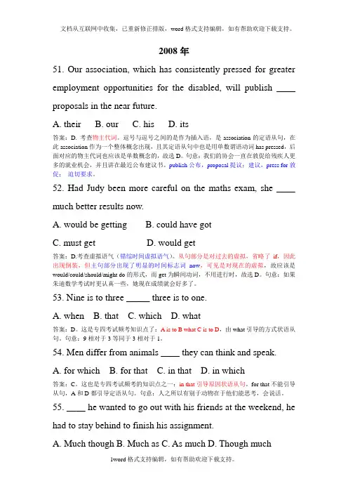
2008年51. Our association, which has consistently pressed for greater employment opportunities for the disabled, will publish ____ proposals in the near future.A. theirB. ourC. hisD. its答案：D. 考查物主代词。

逗号与逗号之间的是作为插入语，是association的定语从句，在此association作为一个整体概念出现，且其定语从句中也是用单数谓语动词has pressed，后面对应的物主代词也应该是单数概念的，故选D。

句意：我们的协会一直在敦促给残疾人更多的就业机会，并且讲在最近公布建议书。

publish公布，proposal提议；建议，press for敦促；迫切要求。

52. Had Judy been more careful on the maths exam, she ____ much better results now.A. would be gettingB. could have gotC. must getD. would get答案：D.考查虚拟语气（错综时间虚拟语气）。

从句部分是对过去的虚拟，省略了if，因此出现倒装，但主句部分出现了明显的时间标志词now，可见是对现在的虚拟，故应该是would/could/should/might do的形式，而get为瞬间动词，不用进行时，故选D。

句意：如果朱迪数学考试时更认真一些，她现在成绩就会好多了。

53. Nine is to three _____ three is to one.A. whenB. thatC. whichD. what答案：D。

这是专四考试频考知识点了：A is to B what C is to D，由what引导的方式状语从句。

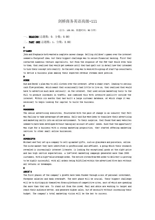
剑桥商务英语高级-111(总分：100.00，做题时间：90分钟)一、READING(总题数：0，分数：0.00)二、PART ONE(总题数：1，分数：8.00)AE-GAMESJohn and Stephanie both wanted a complete career change. Selling children's games over the internet seemed a foolproof idea, but their biggest challenge was to secure financial backing. First they contacted numerous venture capitalists, but from the response of the few that would even talk to them, they realised they would get nowhere until they had spelt out in detail how they intended to turn their concept into reality. So the next step was to work with a group of start-up consultants, to devise a business plan making their expected revenue streams more precise.BSUREKSue and Derek's plan was to sell clothes over the internet. After a shaky start, leading to serious cash flow problems, which meant they occasionally had little to live on, they realised they would have to advertise much more seriously: on the internet, they used online marketing tools to the full to produce increases in traffic, and combined this with intensive publicity outside the internet. Within six months they had built a large customer database, at which stage it was necessary to begin looking for capital to build the business.CWONDERWEBTwo senior advertising executives, frustrated with the pace of change in an industry they felt was failing to take advantage of new media, Sally and Sue were keen to translate their advertising and marketing skills into an online environment. To their surprise, they found that many websites seemed to have been developed without taking any account of users' needs. Sure that the opportunity was ripe for a business with a strong marketing proposition, they started offering marketing services to other small online businesses.DSUPERGIFTSMichael and Tony set up a company to sell up market gifts, such as glassware and porcelain, online. The niche market they have identified is professional and affluent, a group which their research revealed is increasingly internet literate, is looking for exceptional goods at the right price and has high service expectations. A low-level marketing campaign generated more than 2000 customers, with a high-value average order. The entire system from web order to delivery is proving to be highly successful, with all orders being fulfilled within the advertised five days without any returns or breakages.EABBIE'SThe first phases of the company's growth have been funded through a mix of personal investment, foregone salaries and bank overdraft. The next phase will be crucial. Their biggest challenge will be to distinguish themselves from a plethora of competitive sites, most of which are spending far more than they are. To stand out from the crowd, Paul and Abbie are working to target and reach their audience better, and generate higher sales, but of necessity without increasing their budget. The company's total marketing vision will be the key to success.（分数：8.00）(1).These people have not paid themselves out of their company's income so far.（分数：1.00）填空项1:__________________ （正确答案：E）解析：(2).These people had knowledge which they wanted to exploit in a different type of company.（分数：1.00）填空项1:__________________ （正确答案：C）解析：(3).These people's initial efforts to obtain start-up funding were unsuccessful.（分数：1.00）填空项1:__________________ （正确答案：A）解析：(4).These people have developed a very effective process for handling sales.（分数：1.00）填空项1:__________________ （正确答案：D）解析：(5).These people devised a mixed media approach to advertising.（分数：1.00）填空项1:__________________ （正确答案：B）解析：(6).These people felt that they could improve companies' focus on customers.（分数：1.00）填空项1:__________________ （正确答案：C）解析：(7).These people intend to make their marketing more cost-effective.（分数：1.00）填空项1:__________________ （正确答案：E）解析：(8).These people are targeting a relatively small number of discerning clients.（分数：1.00）填空项1:__________________ （正确答案：D）解析：三、PART TWO(总题数：1，分数：6.00)Shoppers wary of 'premium' goodsOne of the marketing industry's favourite terms is 'premium' - usually taken to mean 'luxury' or 'top quality'. The ideal is to create a premium car, wristwatch or perfume - something that appears to transcend the ordinary. When they succeed, marketers are able to charge high prices for the resulting product.However, manufacturers should take note of a recent survey of shoppers' attitudes to so-called premium goods. (9) In fact, the tag seems to have become devalued by overuse.Consumers of all socio-economic backgrounds are very keen to buy the best - but not all product categories lend themselves to a premium status. 'Premium' can be used in any category where image is paramount, and that includes cars, toiletries, clothes and electronics. (10) Banking and insurance are typical of this second group.More than 70 per cent of consumers interviewed in the survey said that a premium tag on everyday items such as coffee or soap is an excuse to charge extra for products that don't always have extra benefits. (11) The prevalence of such a suspicious attitude makes life hard for the marketers. While the word 'luxury' had a clear and definable meaning among respondents - most related it to cars - 'premium' was found to be harder to define. Oddly, the only category apart from cars where 'premium' was understood to mean something specific was bread. (12) Several respondents said they would never pay much for a standard sliced loaf but on special occasions would happily pay double for something that qualifies as a treat.Packaging was found to be an important factor in charging extra for premium products, with sophisticated design enabling toiletries, electronics or food items to sell for far more. Shoppersare willing to pay extra for something that has had thought put into its outward appearance. (13) Yet the knowledge has no impact on their choice.The profit margin on premium-priced toiletries and beauty items can be as much as 300--400 per cent - and in excess of 500 per cent for hi-fi and other electronic goods. (14) In a crowded marketplace such as cars or mobiles, it's far more difficult to achieve this transformation than you might think.A The term is less effective, however, in areas where style and fashion play a smaller role.B The product hidden behind this attractive exterior may be exactly the same as an item selling for half the price, and shoppers may be quite aware of this.C The results suggest that the term 'premium' means very little to consumers.D A fifth of them went further, and dismissed the very word as simply a way of loading prices.E It follows that price and utility are not the only factors in play when it comes to purchasing decisions.F With such an incentive, the challenge for marketers is to find the triggers that can turn an ordinary product into something consumers will accept as premium.G The survey found that consumers were prepared to pay top prices for speciality items, just as long as prices for everyday products remained low.H When they succeed, marketers are able to charge high prices for the resulting product.（分数：6.00）填空项1:__________________ （正确答案：C）解析：填空项1:__________________ （正确答案：A）解析：填空项1:__________________ （正确答案：D）解析：填空项1:__________________ （正确答案：G）解析：填空项1:__________________ （正确答案：B）解析：填空项1:__________________ （正确答案：F）解析：四、PART THREE(总题数：1，分数：6.00)Bruce Petter has not always been an executive. He started his career pumping petrol at a filling station, as he explains: 'After I left the army, my friend's father, who was Managing Director of a petrol company, recommended that I go into the oil industry. My great- uncle was running our own family petrol company, and I learnt the ropes at a petrol station. I subsequently married the daughter of the Marketing Director but this did not make for the happiest of scenarios. Depending on which side of the family they came from, my relatives thought I should support either my great-uncle or my farther-in-law, so I decided the time had come for me to leave the warring factions to fight it out among themselves and move on.'He became founding Director of the Petrol Retailers Association. But after a few years he decided, 'I was getting to the stage where I wanted to move on again, so when I heard about the Management Consultants Association (MCA) post, I applied.'He was aware that the selection process for the head of any trade association would, by definition, be protracted because of the difficulty of getting very busy people with mainstream business interests together. The association had 30 member companies at the time, representing a large proportion of the best-known names in the sector, and 'they all wanted to have a look at this individual who had applied to represent their interests, so I saw an awful lot of the membership'.His principal area of expertise, he feels, is in running a trade association and the briefing that he has been handed suggests that this will be of prime value. 'If you were to ask me if I was ever going to be an expert management consultant, the answer would be no. But I am, I hope, able to articulate their views, to push through policies they want to see in operation and to improve their image. I hope to make management consultancy a powerful voice in government and industry.'The President of the MCA confirms what landed Petter the job. 'We saw a lot of people, but there were three things in particular that impressed us about Brace. His experience of running a trade association was key and it seemed to us that he had a good understanding of how to relate to and inspire a membership made up of very busy partners, often in very large but also some considerably smaller firms. We are also aware that management consultancy is not always portrayed in a favourable light and he has done quite a bit of work on public image and has some very positive views in this area.'So, Mr Petter has taken over from retiring Director Brian O'Rorke, and a change of mood is now in the air. O'Rorke was at the helm for 13 years and his successor is reticent when it comes to predicting how his own approach will differ. 'Brian did a magnificent job of sustaining the Association, of holding it together through thick and thin.' I detect a 'but' in his voice. But? 'I think if you ask anybody who or what the MCA was under his direction, the temptation would be to say "Brian O'Rorke". 'Petter feels his own style will be very much determined by the objectives of the members: he sees himself as a channel for those aims. 'I don't want the MCA to be perceived as Bruce Petter's empire, but rather the members' empire,' he says. Mr Petter clearly has a difficult task ahead, but many of his staff will welcome a more open, modem style and there's every indication he will be a success.（分数：6.00）(1).What do we learn about Bruce Petter in the first paragraph?（分数：1.00）A.He likes to think of himself as a loyal person.B.He has a negative view of family-run businesses.C.His military background came in useful later in his career.D.An awkward situation influenced the development of his career. √解析：(2).When Petter applied for the post of Director of the MCA, he knew that（分数：1.00）A.a decision was likely to take a long time. √B.not everyone in the Association was interested in him.C.he would have to face intense competition.D.some members would oppose his appointment.解析：(3).What does Petter believe he is able to change?（分数：1.00）A.the views the MCA holds on industryB.the way in which the MCA decides on policyC.how the MCA is perceived by other people √D.the MCA's relations with other trade associations解析：(4).Which of the following does the MCA President mention as a reason for appointing Petter?（分数：1.00）A.his ability to motivate members of an association √B.his experience of working in different tradesC.his broad network of business contactsD.his previous work in management consultancy(5).The writer notices that, when Petter talks about his predecessor, he（分数：1.00）A.expresses some regret for how the Association dealt with him.B.thinks he had been there for too long.C.questions changes he made within the Association.D.indicates he has mixed feelings about his leadership styl √解析：(6).Petter says his aim as Director of the MCA is to（分数：1.00）A.modernise the Association.B.carry out the Association's wishes. √C.set an example of firm leadership to his staff.D.expand the membership of the Association.解析：五、PART FOUR(总题数：1，分数：10.00)Sickness at workSmall firms are counting the cost of sickness among employees. Research estimates that illness cost small businesses in Britain a month and a half in lost (21) last year. A recent (22) of more than 1,000 small and medium enterprises revealed that last year the average small business lost around 42 days through staff phoning in sick, and that this had a serious (23) on 27 per cent of smaller companies.Just over one in ten employees took time off for seven days in a(24) Of these, 9.5 per cent were ill for a week on more than one occasion. In Britain, employees can take sick (25) for up to a week before they have to produce a medical certificate. Owner-managers were far less likely to be off sick than their staff: 3.3 days on average, compared with the 10 days taken by employees.The head of the research team said, 'The most common (26) of absence was minor illness, such as colds or flu, but back strain, fractures and the like (27) for very nearly as much. Of greater (28) is that more that 40 per cent of employers felt that their employees' sickness may not have been genuine.'Employers can do more to protect themselves by drawing up adequate (29) of employment that outline the company's sick pay (30) Enhanced sick pay is then at the employer's discretion.（分数：10.00）A.capacityB.productivity √C.capabilityD.efficiency解析：A.reportB.enquiryC.statementD.survey √解析：A.resultB.consequenceC.impressionD.impact √解析：A.row √C.seriesD.sequence解析：A.leave √B.breakC.timeD.absence解析：A.reasonB.symptomC.cause √D.motive解析：A.contributedB.accounted √C.totalledD.credited解析：A.concern √B.anxietyC.regardD.bother解析：A.detailsB.itemsC.particularsD.terms √解析：A.ideasB.notionsC.policies √D.intentions解析：六、PART FIVE(总题数：1，分数：10.00)Employment with Kinson plcStaff Support Advisers requiredWe are a newly-formed division of Kinson plc, one of the UK's largest quoted companies, and provide business customers (31) solutions that combine leading-edge e-commerce technology and an integrated nationwide customer support network.The formation of this new division has created a number of exciting and challenging roles within the call centres of two (32) our seven sites. We have vacancies (33) Staff Support Advisers. Working closely with the Business Managers, your job will (34) to gear the business up for the challenges ahead by implementing a programme of radical change. When completed, this programme will enable the management team to use our people resources more effectively, and (35) so doing facilitate the implementation of our company's business plan. You will be involved in all aspects of human resources activity, including providing advice and guidance to your business partners and policy development, in (36) to implementing any training and development initiatives the company may launch from time to time.We are looking for talented individuals (37) good generalist grounding has been gained in a customer services or customer-focused environment where your flair and ideas (38) currently being underused. You must be able to influence business decisions from a human resources perspective and create innovative solutions. You should also be a resilient, adaptable team player, as (39) as having a track record of coaching others. In return, an excellent salary and benefits package is (40) often The successful applicant will have the advantage of outstanding opportunities for personal development and advancement.（分数：10.00）填空项1:__________________ （正确答案：WITH）解析：填空项1:__________________ （正确答案：OF）解析：填空项1:__________________ （正确答案：FOR）解析：填空项1:__________________ （正确答案：BE）解析：填空项1:__________________ （正确答案：BY/IN）解析：填空项1:__________________ （正确答案：ADDITION）解析：填空项1:__________________ （正确答案：WHOSE）解析：填空项1:__________________ （正确答案：ARE）解析：填空项1:__________________ （正确答案：WELL）解析：填空项1:__________________ （正确答案：ON）解析：七、PART SIX(总题数：1，分数：12.00)CHIEF EXECUTIVE’S REVIEWThe prime focus for management recently has been the integration into the Group ofDamon Beds. This acquisition is very much greater part of our strategy to grow our41 presence in the UK branded furniture market. We are neither convinced that42 leveraging the proven brand management expertise of which we are proud is the43 optimum route to continued and sustainable growth in shareholder value. Overall,44 sales grew more quickly than 9%, to reach ￡125 million. This represents a small45 increase in market share such as our strategy to build share in growing, added value46 sectors gains momentum. Our established brands had another excellent year with47 volumes and turnover at record levels. While we have increased capacity to cope with48 significantly increased demand, boosted by the return to television advertising in early49 last year. The purpose of the campaign is how to reinforce our position as the UK's50 leading volume bed business by improving brand awareness still further on and, more51 importantly, communicating to consumers regarding the message about the uniqueness52 of the product and yet the benefits and reasons for choosing our beds. Earlyindications show that the campaign is already having the desired effect.（分数：12.00）填空项1:__________________ （正确答案：NEITHER）解析：填空项1:__________________ （正确答案：CORRECT）解析：填空项1:__________________ （正确答案：CORRECT）解析：填空项1:__________________ （正确答案：QUICKLY）解析：填空项1:__________________ （正确答案：SUCH）解析：填空项1:__________________ （正确答案：CORRECT）解析：填空项1:__________________ （正确答案：WHILE）解析：填空项1:__________________ （正确答案：IN）解析：填空项1:__________________ （正确答案：HOW）解析：填空项1:__________________ （正确答案：ON）解析：填空项1:__________________ （正确答案：REGARDING）解析：填空项1:__________________ （正确答案：YET）解析：八、WRITING(总题数：0，分数：0.00)九、PART ONE(总题数：1，分数：2.00)（分数：2.00）__________________________________________________________________________________________ 正确答案：(Sample AREPORTThis pie chart shows the number of employees in each factory in the year 2003. The factory in Bristol has the most employees with a number of 600. The factory in Leeds has 350 employees and finally, London employs 150 employees. Bristol made each quarter most of the profits also if it is slowly going down during the year. The profits in Leeds remain stable except for the 3rd quarter where the profits decreased but not dramatically. The factory in London has the worse profits, but they reached a high in the 2nd quarter. Afterwards the profits remain stable. As a result we can see that more the number of employees in the factory is high, more it will have a positiv impact on the profit.Band 3This is a simplistic answer, but the range of structure and vocabulary is nevertheless adequate for the task and there are minimal errors. The target reader would be informed about the trend in profits.Sample BThis report outlines the development of profits in three plants, in London, Leeds and Bristol, in 2003 and describes the staffing situation in each plant.Bristol, the company's largest factory, employed 600 people and reached profits of ￡12 millionin the first quarter of 2003. The profits declined steadily, dropping to ￡9 million in the last quarter.The factory in Leeds had a workforce of 350 people. This made it the company's second largest plant. Profits remained almost unchanged at ￡8 million. In the third quarter however, they reached a low at ￡7.5 million. The London factory's workforce comprised 150 people. Profits did not vary much and remained just over ￡3 million. Nevertheless, they peaked in the second quarter with earnings exceeding the ￡4 million level.Band 5This is a virtually flawless answer, which fits all the descriptors for a band 5.)解析：十、PART TWO(总题数：3，分数：6.00)2.· This year, your company has used an advertising agency to promote your products or services. Your boss has asked you to write a report about the advertising campaign which the agency arranged. · Write the report for your boss:· out lining what the advertising campaign consisted of· indicating what you feel the strengths and weaknesses of the campaign were· explaining how successful you feel the advertising has been· suggesting ideas for future advertising.（分数：2.00）__________________________________________________________________________________________ 正确答案：(Sample CIntroductionThis report sets out to illustrate the strengths and weaknesses of our advertising campaign and recommend the appropriate version for future advertising.FindingsIn order to generate the competitive advantage in today's hyper-competitive globle market, we had successfully engaged a well-known advertising agency who has delivered its job perfectly. As the arrangement of our agency, we have attened an exhibition.They have produced a series of pop advertisement show on television as well as building up a commercial web successfully. There are tremendous benefits have been generated by taking that three action.1. Through attending the well-know exhibition, not only we have increased the awareness of our customer, but also we haved demonstrated our product of new type mobile phone to their best advantages.2. We have successfully built up the image of American myth among our target group - young generation through the vivid television shows our product is already the symbol of dynamic energetic image.3. Our customers have gain a easier access to us by visiting our newly launched web-site through which they can access to our automated order system and again the date they need.On the other hand, the advertising campaign also exist some disadvantages.1. The advertisement on television has narrowed the range of our customers. Not only the robust young generation should be taken account of the advertisement producing but also the dynamic business executives should be involved in our consideration.ConclusionsThe advertising campaign has increased the customers' awareness and generated the sales, foster tremendous potential customers and enhanced our reputation effectively. Most importantly, all of these three ways of advertising have present our product effectively and buit up ourdistinguished image among customers. The weakness also exist in narrowing our target customers. RecommendationWe should renew our contract of with our advertising agency and lure them to enlarge our image among the aggressive businessman and perfect our web advertising by giving our customers more tools to make them magement their relationship with us.Band 2This is an ambitious attempt at the task, particularly in terms of vocabulary. However, it is marred by numerous errors, which obscure communication. This lack of clarity has a negative effect on the reader.Sample DBackground and purpose of the report Our company, Fish-pro Ltd, carried out an advertising campaign in summer 2004 in co- operation with advertising agency RGS Ltd. Aim of this report is to evaluate how succesfully the campaign was carried out and also to asses main points which need to be taken into account when organising summer 2005 campaign.Content of the campaignIn the campaign three different methods were used when the customers were approached. Firstly, the current customers of Fish-pro were contacted by sending them a letter including a catalogue presenting all the new products Fish-pro has available. In, addition the general public was approached by the use of two mass medias: magazines and the radio.Strengths and weaknesses of the campaignThe strength of the campaign was that by using three different methods to approach the current and prospective customers, Fish-pro was able to reach an audience of 100,000 future customers. In addition, according to the survey made withing the current customers after the campaign, Fish-pro strengthened its image as the number one store of proffessional fishing equipment. The weakness of the campaign according to the survey and according to my personal view was that the campaign was very similar to the campaigns that the competitors of Fish-pro have introduced earlier. Therefore it is not certain that Fish-pro is able to increase its market share in the highly competative fishing equipment markets.Future advertising campaignsWhen starting to prepare the summer 2005 campaign I suggest that Fish-pro would carry out a more visible and in certain ways more 'aggressive' campaign compared to the 2004 campaign.Band 4This is a very well-organised answer with fairly natural use of language and a good range of structures. However, the final content point is not well developed and there are a number of errors.)解析：3.· You have seen the following advertisement and you want to enter your organisation for the award.Most Improved Organisation AwardIf your organisation has made improvements in the last year affecting employees and customers, write and tell us about them. The most improved organisation will win a silver cup and money to help pay for a further improvement benefiting staff.· Write your letter to the competition secretary, Michael James:· introducing your organisation and saying what it does· describing improvements your organisation has made in the last year which have affected staff and customers· saying how you would spend the prize money to benefit staff.（分数：2.00）__________________________________________________________________________________________ 正确答案：(Sample EGeneva, the 27th November 2004Dear Sir,I am writing regarding the advertisement called 'Most Improved Organisation Award.'I work in a bank in Geneva. We are specialized in private banking.Our organisation made big improvements for handicaped people last year.They rebuilt the building to order to make it accessible to wheelchairs. But they also engaged two deaf and two blind people. Being next to those people several employees asked to learn their language. The bank then organised lessons for braille and sign language.This new experience touched many clients and the building is now accessible for everybody. Furthermore, there is a new positive motivation and atmosphere inside the organisation.If the bank win the price, we will reinvest the money into advertisement for disabled people and we will create a foundation. We would like help people to communicate and to help handicaped people to find interesting jobs. It will be a hard task but a nice one.I hope that you will be touched by the effort made.If you have any requests or need any further information, please do not hesitate to call me.I look forward to hearing from you and remain,Yours faithfully,Franqoise DupontSenior Private BankerBand 3This is a safe, umambitious answer, which fulfils all the criteria for a band 3.Sample FDear Michael James:I've read the information of Most Improved Organisation Award in newspapers and feel it a good opportunity for my organisation. Well, our organisation is not for profit. The aim of my organisation is to help those animals which need help. We treat those lovely animals as our good friends because we think life is also important to those animals although they could not speak. With development of industry, the level of life of us human beings has improved a lot while that to those animals is getting worse and worse. During last year, we have saved about 1,000 kinds of animals. When finding a dying animal, we immediately send it to the animal hospital and then take good care of it. When the animal recovers, we actively get touch with those kind people who are willing to help or animal organisations. After sending those lives to related people or organisations, we leave our telephone number and keep touch with them. As far as we know, 80% of animals we saved have been leading a happy life while the others have died for age.Every member of my organisation is perfect. They are kind and warm-hearted. Through our efforts, more and more people have come to realize that animals also have the same right of living as our human beings.Comparing with those organisations for profit, I don't dare to say how much profit my organisation has reiceived. But I think profit is not the only factor in the award, isn't it?If we are honored enough to gain the award, we'll spend all the award on investment on animal hospitals and animal medical care.I believe that what we are doing is a good deed and we also believe that our organisation is the most improved one!We're waiting for your reply and please contact me on 241989 during business hours. Thank you. Yours,。

就业歧视英语作文Title: Employment Discrimination: A Persistent Issue。

Employment discrimination remains a significant challenge in today's society, despite various efforts to address it. Discrimination in the workplace can take many forms, including but not limited to, race, gender, age, disability, and language proficiency. In this essay, wewill focus on the issue of English language proficiency discrimination.First and foremost, it is essential to acknowledge that proficiency in English is often seen as a prerequisite for many jobs, especially in multinational corporations or industries with a global reach. While English proficiency can indeed be advantageous in such contexts, it should not be used as a basis for discriminating against individuals who may not be native English speakers or who may have varying levels of proficiency.One of the most common manifestations of English language discrimination in the workplace is during thehiring process. Many employers specify English proficiency as a requirement for certain positions, often without considering whether such proficiency is genuinely necessary for the job at hand. This practice not only excludes qualified candidates who may be proficient in other languages but also perpetuates systemic inequalities, particularly for immigrants and non-native English speakers.Moreover, even after being hired, employees who do not meet arbitrary English language standards may face discrimination in terms of job assignments, promotions, and opportunities for career advancement. This not only affects the individual's professional growth but also contributesto a hostile work environment where certain employees are made to feel inferior based on their language abilities.It is crucial to recognize that language proficiency does not equate to competence or intelligence. Many individuals who may not be fluent in English are highly skilled and capable workers who can contributesignificantly to their organizations if given the chance. Employers must prioritize skills, qualifications, and experience over language proficiency alone when making hiring and promotion decisions.Furthermore, workplace policies and practices should be inclusive and accommodating of employees with diverse linguistic backgrounds. Employers can implement measures such as providing language training programs, offering multilingual support services, and fostering a culture of respect and acceptance for linguistic diversity. By doing so, organizations can harness the full potential of their workforce and create a more equitable and inclusive workplace environment.In addition to actions taken by employers, policymakers also have a role to play in addressing employment discrimination based on English language proficiency. Legislation and regulations should be enacted to prohibit discriminatory practices in hiring, promotion, and workplace treatment based on language. Furthermore, government agencies and advocacy groups can provideresources and support to individuals who have experienced discrimination and empower them to assert their rights in the workplace.In conclusion, employment discrimination based on English language proficiency is a persistent issue that undermines the principles of fairness, equality, and meritocracy in the workplace. It is imperative for employers, policymakers, and society as a whole to recognize the value of linguistic diversity and take proactive measures to combat discrimination in all its forms. Only by fostering inclusive and equitable workplaces can we fully realize the potential of every individual and build a more just and prosperous society.。

在工作中应该禁止年龄歧视的英语作文全文共6篇示例，供读者参考篇1Age Discrimination at Work is Really Unfair and BadMy name is Billy and I'm 10 years old. Today I want to tell you why I think age discrimination in the workplace is really unfair and bad and shouldn't be allowed.What is age discrimination? It's when someone is treated differently or not given the same opportunities just because of their age. For example, an older person might not get hired for a job they are qualified for just because the employer thinks they are too old. Or a younger person might not get promoted because their boss thinks they are too young and inexperienced. That's age discrimination and it's wrong!Imagine if you worked really hard at your job, showed up on time every day, did great work, and never got in trouble, but then you didn't get a promotion just because of your age. That wouldn't be fair at all! You should get opportunities at work based on your skills, experience, qualifications and how well youdo your job - not on how old or young you are. Age shouldn't matter if you are amazing at your job.Older workers have tons of valuable knowledge from all their years of experience. They can teach younger employees so much. And younger workers have fresh ideas and energy. Both older and younger workers have important strengths that make them good employees. Workplaces should value all their workers no matter their age.Age discrimination can really hurt people's feelings and make them feel bad about themselves for no good reason. If you are treated worse just because of your age, it's hurtful and demoralizing. No one should have to feel that way at their workplace. We all deserve to be treated with respect.Not only is age discrimination unfair and mean, it's also really dumb for companies. If they discriminate against someone just for being older or younger, they could be missing out on hiring or promoting amazing employees who would help the company be successful. That's like shooting yourself in the foot! Companies shouldn't limit their talent pool for silly reasons like age.There are laws in some places that make age discrimination illegal, which is good. But age discrimination still happens a lot,which is bad. We need stricter laws to totally ban and punish age discrimination so it stops happening everywhere.I asked my grandpa about this and he told me that when he was younger, age discrimination was even more common and accepted, which is crazy! He said older workers used to get pushed out of their jobs and denied opportunities just for being older, even if they were great at their job. Can you imagine?? That's so messed up. Thankfully things have gotten a little better, but we still have more work to do.My grandpa's friend Mr. Thompson was an amazing engineer but he lost his job right before he could retire just because his company thought he was too old, even though he was awesome at his work. That's horrible! Mr. Thompson had to struggle to find a new job and delay his retirement because of the company's unfair age discrimination. Stories like that make me sad and angry.On the flip side, I know some young people who are incredibly hard workers but don't get taken seriously just because they are younger. My aunt is only 25 but she's wicked smart and always gets great reviews at her job. But she hasn't been promoted yet because her old fossil boss thinks she's too young and inexperienced, even though she works her tail off.That boss is just being a big jerk with his dumb age discrimination.Whether someone is 25 or 65, they should get the same opportunities as everyone else if they are qualified and do amazing work. Age discrimination is unfair, hurtful, and dumb. We need to ban it completely through strict laws with major punishments for companies that discriminate so everyone gets treated fairly no matter their age.At the end of the day, it doesn't matter if you're 25 or 65 - what matters is the quality of your work and contributions. That's what companies should care about, not someone's age. If you're great at your job, you deserve opportunities. Age discrimination needs to be obliterated so we can all get hired, get promoted, and get treated with respect based on our skills and hard work, not on how old or young we are. We're all human beings who deserve fairness at work no matter our age. It's that simple!Age discrimination is really unfair, dumb, and mean. Let's get rid of it forever so all workers of all ages can feel good and be judged only by the awesomeness of their work, not by their age. Thanks for reading my essay! I hope it convinced you that age discrimination in the workplace is whack and needs to be banned with strict punishments. We can and must end agediscrimination once and for all through stronganti-discrimination laws. The end.篇2Age Discrimination at Work is Not Fair!Have you ever noticed that some people treat others differently just because of their age? It's not right and it's called age discrimination. Age discrimination happens when someone is treated unfairly because they are younger or older. Just like it's not okay to treat someone badly because of their skin color or gender, it's also not okay to judge or mistreat someone for being a certain age.At school, the teachers are not allowed to be mean to students just for being younger or older than others. The same rules should apply at work too! Whether someone is a fresh graduate just starting their career or a seasoned employee with decades of experience, they deserve to be treated with equal respect and given the same opportunities as everyone else who is doing a good job.I really don't like age discrimination because it can lead to some very unfair situations. An older worker who is amazing at their job could get passed over for a promotion, just becausetheir boss thinks they are "too old" even though they work super hard. That's not right at all! Or a young person fresh out of college could have a tough time getting hired for an entry-level position because employers think they are "too young" and "inexperienced," even if they are really smart and eager to learn. No one should be judged just for their age!People of all ages have valuable skills, experiences, and perspectives to contribute at their jobs. Older employees often have deep knowledge, proven leadership abilities, and strong work ethics that make them extremely valuable. And younger employees can bring new energy, creativity, and tech-savvy skills that are so important these days. At their best, workplaces should blend the diverse talents of employees from different age groups. Everyone benefits when age diversity is respected and valued.But age discrimination gets in the way of creating positive workplaces that celebrate our differences. It breeds unfair treatment, hurts morale, and deprives companies of top talent just because of someone's age group. That's why I believe age discrimination needs to be fully prohibited to protect workers' rights and allow the best employees to thrive, no matter their age.I think there should be strict laws against age discrimination, just like there are laws against discriminating based on race, religion, gender and disability status. Companies should never be allowed to consider age when hiring, promoting, or deciding who gets opportunities and whose jobs are secure. It should be totally illegal to make employment decisions based on arbitrary age factors rather than employees' skills, qualifications and job performance. With clear anti-discrimination laws and trainings in place, people would be protected against being treated unfairly due to age bias.There's no good reason to allow age discrimination to keep happening in today's workplaces. Young or old, we all deserve to have equal chances to work hard and achieve our career dreams without facing hurtful age stereotypes or restrictions. So let's put an end to unfair treatment based on age, and make sure all workers have opportunities to use their unique talents regardless of how many years they've been alive. A more age-inclusive workforce is a stronger, smarter, and much more just workforce for all of us.篇3Why Old People Shouldn't Be Treated Badly at WorkHave you ever noticed how grown-ups sometimes treat really old people differently than younger people? Maybe they talk down to them like they're babies, or make jokes about them being forgetful or moving slowly. That's called age discrimination, and I think it's really mean and unfair.Old people have just as much value as anyone else. They've been around a long time and seen and done so many things, so they're actually a lot wiser than young folks in many ways. My grandma knows everything about gardening and can grow the most amazing tomatoes. And my grandpa can fix anything - cars, appliances, you name it. Their generations invented most of the useful things we use today!But some people act like just because old people move a little slower or have wrinkly skin, they must not be very smart or capable anymore. That's not true at all! Sure, some old people do get a little more forgetful or have health problems as they age. But so do lots of young people. We're all human and all have our own strengths and weaknesses no matter how old we are.At work, older people bring so much experience and knowledge that younger people just don't have yet. They've been working hard their whole lives, so they definitely know what they're doing. A business would be crazy not to value thosekinds of skilled, hardworking employees just because of their age.Can you imagine if someone didn't hire you for a job you really wanted just because of how old you are? Or if your boss passed you over for a promotion, and gave it to someone younger instead, even though you're way better at the job? That would be so unfair and dumb!Unfortunately, that kind of age discrimination happens a lot. Many workplaces look down on older workers and choose not to hire or promote them just based on their birthdays. Some companies even force people to retire at a certain age, which is absolutely ridiculous if the person is still able to work just fine.Older workers have mortgages and families to support, just like everyone else. Forcing them out of a job they're great at just because of their age can make their lives really difficult. That's just mean and disrespectful after everything they've contributed to society over the decades.What's worse is that age discrimination is still legal in many places! Can you believe that? In those places, bosses are actually allowed to reject someone for a job solely because they have grey hair or are over a certain age. That's so backwards! Age is just a unavoidable fact of life, not some kind of bad quality.If someone is qualified for a job and good at it, their age shouldn't matter at all. An 80-year-old professor isn't automatically worse at teaching just because of their age. A70-year-old carpenter has way more building skills than a new kid on the construction site. We should be appreciating their valuable experience, not pushing them out just for getting older!In my opinion, age discrimination in the workplace is totally unacceptable and should be banned everywhere. Employees must be judged only on their work performance and qualifications for the job - not on how many birthdays they've had. That's only fair. Older people deserve the same rights, job opportunities, and respect as everyone else.Just imagine how you would feel as an old person getting turned down for a job you're fully capable of just because the boss thinks you're too old and fragile. You'd feel absolutely horrible and disrespected after working so hard your whole life. No one should have to go through that kind of hurtful discrimination just for growing older.Growing old is a natural part of life that happens to all of us if we're lucky enough. Older people have so much to teach us and so many amazing life experiences to share. They've helped build this world for young people like me. The very least we cando is treat them with kindness, equality and respect in the workplace - not make them feel like disposable items just for getting wrinkles and grey hair.I really hope that protective laws against age discrimination in hiring, promotion and forced retirement become standard everywhere. Until then, we should all make an effort to appreciate older workers and everything they have to offer. Just because someone is old doesn't make them any less smart, skilled or hardworking. Judge people based on what's actually important - their character and abilities - not their age. Discriminating against elders is plain wrong and hopefully will soon be illegal everywhere it still sadly exists.篇4Age Discrimination is Really Not Fair at Work!Hi there! My name is Jamie and I'm 10 years old. Today I want to talk to you about something that I think is super unfair and needs to stop - age discrimination in the workplace. What does that mean? Well, it's when people get treated differently at their jobs just because of how old they are. Older people and younger people can both face this kind of discrimination. It's not right at all!Let me give you some examples to explain what I mean. Let's say there's a company that needs to hire someone new. Two people apply for the job - one is 25 years old and the other is 55 years old. They both have the same exact qualifications and experience. But the company decides to hire the 25 year old instead of the 55 year old just because they think the younger person is "a better fit." That's age discrimination against the older worker!Or imagine a workplace where all the older employees get passed over for promotions and raises, while the younger employees keep moving up. The bosses think the younger people are more "dynamic" and have more "energy." But the older workers are just as good at their jobs! That's also age discrimination.Age discrimination can even happen to younger workers too. Some employers think people right out of school are "too inexperienced" or "not mature enough" to handle important jobs. So they only hire and promote people older than 30 or 35. That's discrimination against younger people based only on their age, not their actual skills.No matter if it's happening to older or younger people, I think age discrimination at work is completely unfair. A person'sage doesn't determine how good they'll be at their job. There are awesome workers of ALL ages! People should be hired, promoted, and treated based only on their qualifications, experience, and how well they perform - not their date of birth.When companies discriminate like this, they could be missing out on hiring or keeping their very best people. They're judging books by their covers instead of the contents inside. That's just silly! Older people bring so much experience and wisdom to jobs. And younger people have fresh perspectives and new ideas. Workplaces should value what all generations have to offer.Plus, discriminating against people for something they can't control, like their age, is just plain mean. It can really hurt people's feelings and make them feel bad about themselves for no good reason. Nobody should have to experience that at their workplace. Jobs should make people feel happy and valued, not inferior because of their age.If people of all ages are allowed to get hired and promoted fairly, it creates awesome diverse workplaces. That's good for employers because diversity leads to better problem solving. It's also good for workers because they can learn a ton from peopleof different ages and backgrounds. Mixing it up makes everything better!I really hope that countries all around the world make laws to completely ban age discrimination at work. Nobody's age should hold them back from getting hired somewhere, doing their best work, and earning promotions and raises they deserve. We need to create workplaces that are fair for everyone, no matter their age.We should judge people only by their character, talents, and work ethic - NOT by their number of birthdays. An awesome23-year-old employee deserves the exact same opportunities as an awesome 67-year-old employee. That's what true fairness and equality means. Age doesn't define people, it's just a number!So let's fight to end this unfair age discrimination in the workplace everywhere. Whether you're a kid, a teenager, a young adult, a middle-aged person, or a senior citizen - you deserve to get an equal chance. We're all human beings who want to work hard, support our families, and live happy lives. Don't let anybody's age get in the way of that!篇5Age Discrimination Should Be Banned in the WorkplaceHave you ever heard of age discrimination? It's when someone is treated unfairly because of how old they are. I think age discrimination in the workplace is really mean and it should be banned!What is age discrimination? It's when older workers are not given the same chances as younger workers, just because of their age. Or sometimes, younger workers get treated badly too, just for being young! This happens when bosses won't hire people, give them promotions, or treat them with respect just based on how old they are.I think age discrimination is super unfair. A person's age doesn't mean they are a good worker or a bad worker. We shouldn't judge people just by a number! There are great workers of all ages - young and old.Instead of looking at age, employers should look at someone's skills, experience, and how hard they are willing to work. Those are the things that really matter when it comes to being a good employee. Not how many years they've been alive!Imagine if you worked really hard at your job, showed up on time, did great work, and were kind to everyone. Then someone younger than you gets promoted over you, just because they are younger! That wouldn't be fair at all. You should get thatpromotion because of your hard work and experience, not because of your age.Or what if you were looking for your first job and all the bosses said "Sorry, you're too young and too inexperienced for this job." Before you even got a chance to show what you could do! That's age discrimination against younger people, and it's not right.Everyone deserves a fair chance at a job, no matter their age. Older people have valuable experience that can help a company. And younger people have fresh ideas and energy to bring to the workplace. Companies should want workers of all ages to create a diverse and dynamic team.Not only is age discrimination unfair, but I think it's also illegal in many places. That means it's against the law to treat someone differently at their job just because of how old they are. There are laws that protect workers from this kind of unfair treatment.However, age discrimination still happens a lot, which is really sad. Some employers have negative attitudes towards hiring older workers because they think they can't learn new skills or will cost more in health insurance. That's just wrong! Older workers have lots to offer.And some employers don't like to hire younger workers because they think they are inexperienced or will job-hop to a different company. But lots of young people are hard workers who just need a chance to prove themselves.Ultimately, people of all ages can be great employees if they have the right skills and attitude. Employers should pick the best person for the job, regardless of how old they are. Judging someone just based on their age is discrimination, and it can lead to a company missing out on amazing talent.So in my opinion, age discrimination needs to be banned in workplaces everywhere. It's unfair, illegal, and hurts both companies and workers. We should judge people based on their character, abilities, and work ethic, not their age. After all, you can be an amazing worker at 20 or 65! What matters most is how you treat others and how hard you're willing to work.I hope that when I'm older, age discrimination will be a thing of the past. Everyone deserves a fair chance at a good job, no matter if they are young or old. Hard work and talent should be what counts, not how many birthdays you've had. That's why age discrimination in the workplace has to go! Let's make the world of work a fairer place for people of all ages.篇6Age Discrimination Should Be Banned in the WorkplaceHi friends! Today I want to talk about something very important called age discrimination. Have you ever heard of that before? It's when someone is treated unfairly just because of how old they are. Can you believe that? Just because someone is older or younger, they get treated worse than others. That doesn't seem right at all!Age discrimination happens a lot in the workplace. The workplace is where grown-ups go to do their jobs and earn money. Some bosses and managers don't want to hire older workers or workers who are younger than a certain age. They think older people can't do the job as well or that younger people don't have enough experience. But that's not fair at all!My grandma is 70 years old and she is one of the smartest, most hard-working people I know. She still works part-time at the library and she is amazing at her job. She knows where every book is, she helps all the kids find what they need, and she works really hard. Just because she's older doesn't mean she can't do her job well. That's age discrimination and it's wrong.On the other hand, some companies don't want to hire younger workers right out of school. They think young people are lazy or don't know what they're doing. But lots of young people are very motivated to get good jobs and work hard. My older brother just graduated from college and he's been looking for his first big job. He studied really hard and gets great grades. Just because he's younger doesn't mean he can't be a good worker. Not giving him a chance is also age discrimination.Whether someone is old or young, tall or short, they should be judged only on their abilities to do the job, not their age. It's not fair to say someone can't work somewhere just because of how old they are. That's discrimination, plain and simple.Everyone deserves a fair chance at a good job if they are qualified and can do the work. Grandma has decades of experience from working her whole life. My brother has a brand new degree and learned all the latest skills in school. They both deserve opportunities based on what they can do, not how old they are.Age discrimination can make people feel bad about themselves too. Older workers who get fired or can't get hired might feel sad and useless, like they have nothing left to contribute. That's not right at all! Older people are wise and haveso much knowledge to share. Just because you're old doesn't mean you're no good anymore.Younger workers who face discrimination might also feel hurt and get discouraged. If they keep getting rejected for jobs just because they are young and "inexperienced", they may start to doubt themselves. But everyone has to start somewhere! We were all inexperienced once until we got our first job and learned new things. Younger people deserve a fair shot too.So in the end, I think age discrimination of any kind should be totally banned in the workplace. It's mean, it's unfair, and it hurts people's feelings. What does someone's age have to do with how well they can do a job anyway? There are awesome workers of all ages who deserve respect and opportunities.Companies should look at each worker as an individual and decide if they are right for the job, no matter if they are 20 years old or 80 years old. Skills, experience, motivation, and ability are what really matter, not someone's age. Grandma and my brother are both super workers and it would be wrong for a boss to discriminate against them just based on their age. That's just silly and mean. It's time we stopped age discrimination once and for all!。