Counterparty risk and the pricing of defaultable securities

Financial Markets and Institutions, 8e (Mishkin)Chapter 20 The Mutual Fund Industry20.1 Multiple Choice1) At the beginning of 2013, mutual funds held about ________ of the U.S. stock market was held by mutual funds.A) 30%B) 50%C) 10%D) 70%Answer: ATopic: Chapter 20.1 The Growth of Mutual FundsQuestion Status: Updated from Previous Edition2) The origins of mutual funds can be traced back to the mid to late 1800s in________.A) England and ScotlandB) New York CityC) BostonD) GermanyAnswer: ATopic: Chapter 20.1 The Growth of Mutual FundsQuestion Status: New Question3) ________ intermediation means that small investors can pool their funds with other investors to purchase high face value securities.A) LiquidityB) FinancialC) DenominationD) ShareAnswer: CTopic: Chapter 20.2 Benefits of Mutual FundsQuestion Status: Previous Edition4) Mutual funds offer investors all of the following exceptA) greater-than-average returns.B) diversified portfolios.C) lower transaction costs.D) professional investment management.Answer: ATopic: Chapter 20.2 Benefits of Mutual FundsQuestion Status: Previous Edition5) Mutual fundsA) pool the resources of many small investors by selling these investors shares and using the proceeds to buy securities.B) allow small investors to obtain the benefits of lower transaction costs in purchasing securities.C) provide small investors a diversified portfolio that reduces risk.D) do all of the above.E) do only A and B of the above.Answer: DTopic: Chapter 20.2 Benefits of Mutual FundsQuestion Status: Previous Edition6) ________ enables mutual funds to consistently outperform a randomly selected group of stocks.A) Managerial expertiseB) DiversificationC) Denomination intermediationD) None of the aboveAnswer: DTopic: Chapter 20.2 Benefits of Mutual FundsQuestion Status: Previous Edition7) At the end of 2012 there were over ________ separate mutual funds with total assets over ________.A) 800; $10 trillionB) 7,500; $13 trillionC) 10,000; $10 trillionD) 1,000; $7 trillionAnswer: BTopic: Chapter 20.2 Benefits of Mutual FundsQuestion Status: Updated from Previous Edition8) Most mutual funds are structured in two ways. The most common structure is a(n) ________ fund, from which shares can be redeemed at any time at a price that is tied to the asset value of the fund. A(n) ________ fund has a fixed number of nonredeemable shares that are traded in the over-the-counter market.A) closed-end; open-endB) open-end; closed-endC) no-load; closed-endD) no-load; loadE) load; no-loadAnswer: BTopic: Chapter 20.3 Mutual Fund StructureQuestion Status: Previous Edition9) Which of the following is an advantage to investors of an open-end mutual fund?A) Once all the shares have been sold, the investor does not have to put in more money.B) The investors can sell their shares in the over-the-counter market with low transaction fees.C) The fund agrees to redeem shares at any time.D) The market value of the fund's shares may be higher than the value of the assets held by the fund.Answer: CTopic: Chapter 20.3 Mutual Fund StructureQuestion Status: Previous Edition10) The net asset value of a mutual fund isA) determined by subtracting the fund's liabilities from its assets and dividing by the number of shares outstanding.B) determined by calculating the net price of the assets owned by the fund.C) calculated every 15 minutes and used for transactions occurring during the next 15-minute interval.D) calculated as the difference between the fund's assets and its liabilities. Answer: ATopic: Chapter 20.3 Mutual Fund StructureQuestion Status: Previous Edition11) ________ funds are the simplest type of investment funds to manage.A) BalancedB) Global equityC) GrowthD) IndexAnswer: DTopic: Chapter 20.4 Investment Objective ClassesQuestion Status: Previous Edition12) The majority of mutual fund assets are now owned byA) individual investors.B) institutional investors.C) fiduciaries.D) business organizations.E) retirees.Answer: ATopic: Chapter 20.2 Benefits of Mutual FundsQuestion Status: Previous Edition13) Capital appreciation funds select stocks of ________ and tend to be ________ risky than total return funds.A) large, established companies that pay dividends regularly; moreB) large, established companies that pay dividends regularly; lessC) companies expected to grow rapidly; moreD) companies expected to grow rapidly; lessAnswer: CTopic: Chapter 20.4 Investment Objective ClassesQuestion Status: Previous Edition14) From largest to smallest in terms of total assets, the four classes of mutual funds areA) equity funds, bond funds, hybrid funds, money market funds.B) equity funds, money market funds, bond funds, hybrid funds.C) money market funds, equity funds, hybrid funds, bond funds.D) bond funds, money market funds, equity funds, hybrid funds.Answer: BTopic: Chapter 20.4 Investment Objective ClassesQuestion Status: Previous Edition15) Measured by assets, the most popular type of bond fund is the ________ bond fund.A) state municipalB) strategic incomeC) governmentD) high-yieldAnswer: BTopic: Chapter 20.4 Investment Objective ClassesQuestion Status: Previous Edition16) People who take their money out of insured bank deposits to invest in uninsured money market mutual funds have ________ risk because money market funds invest in ________ assets.A) high; long-termB) low; short-termC) high; short-termD) low; long-termAnswer: BTopic: Chapter 20.4 Investment Objective ClassesQuestion Status: Previous Edition17) The largest share of assets held by money market mutual funds isA) Treasury bills.B) certificates of deposit.C) commercial paper.D) repurchase agreements.Answer: CTopic: Chapter 20.4 Investment Objective ClassesQuestion Status: Previous Edition18) Which of the following is a feature of index funds?A) They have lower fees.B) They select and hold stocks to match the performance of a stock index.C) They do not require managers to select stocks and decide when to buy and sell.D) All of the above.Answer: DTopic: Chapter 20.4 Investment Objective ClassesQuestion Status: Previous Edition19) A deferred-load mutual fund charges a commissionA) when shares are purchased.B) when shares are sold.C) both when shares are purchased and when they are sold.D) when shares are redeemed.Answer: DTopic: Chapter 20.5 Fee Structure of Investment FundsQuestion Status: Previous Edition20) Over the past twenty years, mutual fund fees have ________, largely because________.A) fallen; SEC fee disclosure rules have led to greater competitionB) risen; investors have learned that funds with high fees provide better performanceC) risen; there has been collusion between large mutual fund companiesD) fallen; advances in information technology have lowered transaction costs Answer: ATopic: Chapter 20.5 Fee Structure of Investment FundsQuestion Status: Previous Edition21) Which of the following is most likely to be a no-load fund?A) Value fundsB) Hedge fundsC) Growth fundsD) Index fundsAnswer: DTopic: Chapter 20.5 Fee Structure of Investment FundsQuestion Status: Previous Edition22) When investors switch between funds within the same fund family, mutual funds may chargeA) a contingent deferred sales charge.B) a redemption fee.C) an exchange fee.D) 12b-1 fees.E) an account maintenance fee.Answer: CTopic: Chapter 20.5 Fee Structure of Investment FundsQuestion Status: Previous Edition23) The Securities Acts of 1933 and 1934 did notA) regulate the activities of investment funds.B) require funds to register with the SEC.C) include antifraud rules covering the purchase and sale of fund shares.D) apply to investment funds.Answer: BTopic: Chapter 20.6 Regulation of Mutual FundsQuestion Status: Previous Edition24) The largest share of total investment in mutual funds is inA) stock funds.B) hybrid funds.C) bond funds.D) money market funds.Answer: ATopic: Chapter 20.4 Investment Objective ClassesQuestion Status: Previous Edition25) Over ________ of the total daily volume in stocks is due to institutions initiating trades.A) 70%B) 50%C) 25%D) 90%Answer: ATopic: Chapter 20.6 Regulation of Mutual FundsQuestion Status: New Question26) Hedge funds areA) low risk because they are market-neutral.B) low risk if they buy Treasury bonds.C) low risk because they hedge their investments.D) high risk because they are market-neutral.E) high risk, even though they may be market-neutral.Answer: ETopic: Chapter 20.7 Hedge FundsQuestion Status: Previous Edition27) The near collapse of Long Term Capital Management was caused byA) the high management fees charged by the fund's two Nobel Prize winners.B) the fund's high leverage ratio of 20 to 1.C) a sharp decrease in the spread between corporate bonds and Treasury bonds.D) a sharp increase in the spread between corporate bonds and Treasury bonds.E) the fund's shift away from a market-neutral investment strategy.Answer: DTopic: Chapter 20.7 Hedge FundsQuestion Status: Previous Edition28) Conflicts arise in the mutual funds industry because ________ cannot effectively monitor ________.A) investment advisers; directorsB) directors; shareholdersC) shareholders; investment advisersD) investment advisers; stocks that will outperform the overall marketAnswer: CTopic: Chapter 20.8 Conflicts of Interest in the Mutual Fund IndustryQuestion Status: Previous Edition29) Late trading is the practice of allowing orders received ________ to trade at the ________ net asset value.A) before 4:00 PM; 4:00 PMB) after 4:00 PM; 4:00 PMC) after 4:00 PM; next day'sD) before 4:00 PM; previous day'sAnswer: BTopic: Chapter 20.8 Conflicts of Interest in the Mutual Fund IndustryQuestion Status: Previous Edition30) Market timingA) takes advantage of time differences between the east and west coasts of the United States.B) takes advantage of arbitrage opportunities in foreign stocks.C) takes advantage of the time lag between the receipt and execution of orders.D) is discouraged by the stiff fees mutual funds charge every investor for buying and then selling shares on the same day.Answer: BTopic: Chapter 20.8 Conflicts of Interest in the Mutual Fund IndustryQuestion Status: Previous Edition31) Late trading and market timingA) allow large, favored investors in a mutual fund to profit at the expense of other investors in the fund.B) hurt ordinary investors by increasing the number of fund shares and diluting the fund's net asset value.C) are both A and B of the above.D) are none of the above.Answer: CTopic: Chapter 20.8 Conflicts of Interest in the Mutual Fund Industry Question Status: Previous Edition32) Which of the following is not a proposal to deal with abuses in the mutual fund industry?A) Strictly enforce the 4:00 PM net asset value rule.B) Make redemption fees mandatory.C) Disclose compensation arrangements for investment advisers.D) Increase the number of dependent directors.Answer: DTopic: Chapter 20.8 Conflicts of Interest in the Mutual Fund IndustryQuestion Status: Previous Edition33) ________ means the investors can convert their investment into cash quickly at a low cost.A) Liquidity intermediationB) Denomination intermediationC) DiversificationD) Managerial expertiseAnswer: ATopic: Chapter 20.2 Benefits of Mutual FundsQuestion Status: Previous Edition34) At the start of 2014, one share of Berkshire Hathaway's A-shares was trading at over $150,000. ________ in an mutual fund gives a small investor access to these shares.A) Liquidity intermediationB) Denomination intermediationC) DiversificationD) Managerial expertiseAnswer: BTopic: Chapter 20.2 Benefits of Mutual FundsQuestion Status: Previous Edition35) Mutual fund companies frequently offer a number of separate mutual funds called ________.A) indexesB) complexesC) componentsD) actuariesAnswer: BTopic: Chapter 20.4 Investment Objective ClassesQuestion Status: Previous Edition36) Equity funds can be placed in which class according to the Investment Company Institute?A) Capital appreciation fundsB) World fundsC) Total return fundsD) All of the aboveAnswer: DTopic: Chapter 20.4 Investment Objective Classes Question Status: Previous Edition37) Government bonds are essentially default risk-free, ________ returns.A) and will yield highB) and will yield the highestC) but will have relatively lowD) none of the aboveAnswer: CTopic: Chapter 20.4 Investment Objective ClassesQuestion Status: Previous Edition38) ________ bonds combine stocks into one fund.A) HybridB) Money marketC) MunicipalD) EquityAnswer: ATopic: Chapter 20.4 Investment Objective ClassesQuestion Status: Previous Edition39) All ________ are open-end investment funds that invest only in money market securities.A) Stock fundsB) Bond fundsC) Money market mutual fundsD) all of the aboveAnswer: CTopic: Chapter 20.4 Investment Objective ClassesQuestion Status: Previous Edition20.2 True/False1) The larger the number of shares traded in a stock transaction, the lower the transaction costs per share.Answer: TRUETopic: Chapter 20.2 Benefits of Mutual FundsQuestion Status: Previous Edition2) The increase in the number of defined contribution pension funds has slowed the growth of mutual funds.Answer: FALSETopic: Chapter 20.1 The Growth of Mutual FundsQuestion Status: Previous Edition3) Mutual funds accounted for $5.3 trillion, or 27%, of the $19.5 trillion U.S. retirement market at the beginning of 2013.Answer: TRUETopic: Chapter 20.2 Benefits of Mutual FundsQuestion Status: Updated from Previous Edition4) Among the investors in mutual funds, only about 25% cite preparing for retirement as one of their main reasons for holding shares.Answer: FALSETopic: Chapter 20.2 Benefits of Mutual FundsQuestion Status: Updated from Previous Edition5) Open-end mutual funds are more common than closed-end funds.Answer: TRUETopic: Chapter 20.3 Mutual Fund StructureQuestion Status: Previous Edition6) The net asset value of a mutual fund is the average market price of the stocks, bonds, and other assets the fund owns.Answer: FALSETopic: Chapter 20.3 Mutual Fund StructureQuestion Status: Previous Edition7) A mutual fund's board of directors picks the securities that will be held and makes buy and sell decisions.Answer: FALSETopic: Chapter 20.4 Investment Objective ClassesQuestion Status: Previous Edition8) Money market mutual funds originated when the brokerage firm Merrill Lynch offered its customers an account from which funds could be taken to purchase securities and into which funds could be deposited when securities were sold. Answer: TRUETopic: Chapter 20.4 Investment Objective ClassesQuestion Status: Previous Edition9) A deferred load is a fee charged when shares in a mutual fund are redeemed. Answer: TRUETopic: Chapter 20.5 Fee Structure of Investment FundsQuestion Status: Previous Edition10) Several academic research studies show that investors earn higher returns by investing in mutual funds that charge higher fees.Answer: FALSETopic: Chapter 20.5 Fee Structure of Investment FundsQuestion Status: Previous Edition11) Hedge funds have a minimum investment requirement of between $100,000 and$20 million, with the typical minimum investment being $1 million.Answer: TRUETopic: Chapter 20.7 Hedge FundsQuestion Status: New Question12) SEC research suggests that about three-fourths of mutual funds let privileged shareholders engage in market timing.Answer: TRUETopic: Chapter 20.8 Conflicts of Interest in the Mutual Fund IndustryQuestion Status: Previous Edition13) One factor explaining the rapid growth in mutual funds is that they are financial intermediaries that are not regulated by the federal government.Answer: FALSETopic: Chapter 20.1 The Growth of Mutual FundsQuestion Status: Previous Edition14) Whether a fund is organized as a closed- or an open-end fund, is will have the same basic organizational structure.Answer: TRUETopic: Chapter 20.3 Mutual Fund StructureQuestion Status: Previous Edition15) The primary purpose of loads is to provide compensation for sales brokers. Answer: TRUETopic: Chapter 20.5 Fee Structure of Investment FundsQuestion Status: Previous Edition16) Mutual funds are regulated under four federal laws designed to protect investors. Answer: TRUETopic: Chapter 20.6 Regulation of Mutual FundsQuestion Status: Previous Edition20.3 Essay1) What benefits do mutual funds offer investors?Topic: Chapter 20.2 Benefits of Mutual FundsQuestion Status: Previous Edition2) How is a mutual fund's net asset value calculated?Topic: Chapter 20.3 Mutual Fund StructureQuestion Status: Previous Edition3) How did money market mutual funds originate and why did they become especially popular in the late 1970s and early 1980s?Topic: Chapter 20.1 The Growth of Mutual FundsQuestion Status: Previous Edition4) How does the governance structure of mutual funds lead to asymmetric information and conflicts of interest?Topic: Chapter 20.8 Conflicts of Interest in the Mutual Fund IndustryQuestion Status: Previous Edition5) Describe the practices of late trading and market timing and explain how these practices harm a mutual fund's shareholders.Topic: Chapter 20.8 Conflicts of Interest in the Mutual Fund IndustryQuestion Status: Previous Edition6) Discuss the proposals that have been made to reduce the conflict of interest abuses in the mutual funds industry.Topic: Chapter 20.8 Conflicts of Interest in the Mutual Fund IndustryQuestion Status: Previous Edition7) How is an index fund different from the other four primary investment objective classes for mutual funds?Topic: Chapter 20.4 Investment Objective ClassesQuestion Status: New Question8) Discuss the four primary classes of mutual funds available to investors.Topic: Chapter 20.4 Investment Objective ClassesQuestion Status: Previous Edition9) What are the five benefits of mutual funds?Topic: Chapter 20.2 Benefits of Mutual FundsQuestion Status: New Question10) What is the difference between an open-end and a closed-end mutual fund? Topic: Chapter 20.3 Mutual Fund StructureQuestion Status: New Question11) What are two key differences between a traditional mutual fund and a hedge fund?Topic: Chapter 20.7 Hedge FundsQuestion Status: New Question。

25-9
Futures Markets
• The Chicago Mercantile Exchange (CME) is by far the largest.
• Others include:
– The Philadelphia Board of Trade (PBOT) – The MidAmerica Commodities Exchange – The Tokyo International Financial Futures Exchange – The London International Financial Futures Exchange
25-11
CME After Hours
• Extended-hours trading on GLOBEX runs from 2:30 p.m. to 4:00 p.m dinner break and then back at it from 6:00 p.m. to 6:00 a.m. CST.
OJ Metals & Petroleum
Copper Gold
Unleaded gasoline Financial
British Pound Japanese Yen
Eurodollar
McGraw-Hill/Irwin
Contract Size
Exchange
5,000 bushels 5,000 bushels 10 metric tons
– Its not an option: both parties are expected to hold up their end of the deal.
– If you have ever ordered a textbook that was not in stock, you have entered into a forward contract.

芝加哥大学1.金融数学(1) Background requirementsThere are two main criteria for evaluating applications tothe program, the first is by far the most important:∙ A solid background in Mathematics comparableto a bachelor of science degree in mathematics oranother field of physical sciences is essential. Youshould have solid knowledge of multivariablecalculus, linear algebra and differential equations. If you do not have this knowledge you might look into our Financial Mathematics Preparation Course or courses with similar contents at alocal university. Computer programming ability, especially in Matlab and C++, is also useful and is essential in working afterwards. If you don't have programming experience we recommend that you take the optional course in C++ programming. Some exposure to probability andstatistics is also useful. The biggest reason people are not admitted is inadequate mathematical preparation; it is not possible to "figure it out as you go along."∙We also look at prior industrial experience. A bit of experience has the effect of making you confident that this is the career you really want. This requirement is more flexible than the need for mathematical competence.(2) Application requirementsThere are several application requirements. The application form itself provides more details about each of the requirements.∙Both the GRE General Test and the GRE Math Subject Tests are required. However, if you received your bachelor's degree prior to June of 2007, you are exempt from any GRErequirements.Please consult the GRE website for testing dates, and select dates which will provide results in time for application review. Link to ETS website for GRE testing information.We do not require (and are not interested in) other exam scores, such as GMAT..∙TOEFL. Most foreign applicants must take the TOEFL. The exceptions are students from certain English-speaking countries such as Canada and UK. Please visit the Office of InternationalAffairs website for criteria:https:///students/prospective/toefl.shtml∙Three letters of recommendation. We recommend that even students who have been out of school for a while get at least one recommendation from a professor (preferably a mathprofessor) who can attest to their mathematical abilities.Our institution and department codes for the TOEFL and GRE exams are:Institution Code Department CodeTOEFL Exam 1832 72GRE Exam 1832 0799(3) Contact UsExecutive DirectorWilliam A. DeRonne, Ph.D.Phone: (773) 702-1458Email: bderonne@Career DevelopmentEdonna E. LarkinsPhone: (773) 702-0618Email: elarkins@General InformationAshley DossPhone: (773) 834-4385Email: adoss@Saria BartholomewPhone: (773) 702-1902Email: sariab@Multimedia, Web and ITMichael JehlikPhone: (773) 702-7383Email: mjehlik@(4) Faculty & ResearchHenri Berestycki, DirectorHenri Berestycki is Professor and Director of the Centre d'analyse et de mathematique sociales (CAMS) at the Ecole des hautes etudes en sciences sociales (EHESS) in Paris. He has been a regular visiting faculty member of the Department of Mathematics at the University of Chicago since 2005. He has taught at University Paris VI, Ecole normale superieure and Ecole Polytechnique in France. His research interests include partial differential equations, variational calculus, nonlinear analysis, mathematical models of the financial markets, mathematical models in biology and ecology and modeling in social sciences. Among his many recognitions, this year he was awarded the French Legion of Honor.http://cams.ehess.fr/document.php?id=891William DeRonne, Executive DirectorWilliam DeRonne, Ph.D. has more than 30 years of experience in domestic and international financial markets; most recently he was the President, CEO and Chief Compliance Officer of Fox River Financial Resources. He has experience in all the primary markets as well as their derivatives and has worked in China, Japan and Europe. He managed and directed researchers and traders at TradeLink LLC, Market Liquidity Network, LLC and Chicago Research & Trading. He was Senior Vice President and Director of FinancialEngineering/Quantitative Research and Chairman of the Risk Reviewand Management Committee for Nations Bank.Niels O. Nygaard, Founding DirectorProfessor in the Department of Mathematics at the University of Chicago since 1982. Prior to joining the University of Chicago he taught at Princeton University. He holds a Ph.D. in Mathematics from MIT. Professor Nygaard was the Director of the Financial Mathematics Program since its inception in 1996 until April 2010. Besides his interest in Financial Mathematics he has done research in Arithmetic, Algebraic Geometry and Number TheoryNeil A. Chriss, Advisory DirectorNeil Chriss is the Founder, Chief Investment Officer and CEO at Hutchin Hill Capital, LP. Prior to founding Hutchin Hill in October 2007, Neil was a managing director at SAC Capital Management (2003–2007). Previously, Neil was a portfolio manager at Goldman Sachs Asset Management (1998-2000). In 2000, Neil founded ICor Brokerage, an electronic trading platform for swaps and options, which was subsequently acquired by Reuters Plc. Neil holds PhD and BS degrees in Mathematics from the University of Chicago, and an MS in Mathematics from the California Institute of Technology. He has held academic positions in the mathematics departments of Harvard University, the Institute for Advanced Study, and the University of Toronto. Neil serves in an advisory capacity to the Finance Committee of the Institute for Advanced Study in Princeton, NJ (2008–Present). Additionally, he is a founding board member, and a member of the Executive Committee, of Math for America (2003–Present). Neil is an Advisory Director of the University of Chicago’s Financial Mathematics Program. He also serves on the Board of Trustees at Harvey Mudd College in Claremont, CA. Neil holds a patent for his invention, “Method and System for Portfolio Optimization from Ordering Information”.John ZerolisJohn Zerolis is currently Associate Director of the Program on Financial Mathematics, teaches "Portfolio Theory and Risk Management" (with Jon Frye and Paul Staneski), and is also the founder of Angle Vista LLC, which provides quantitative market and credit risk modeling and training to clients. In the course of his career, he has developed leading edge visualization, simulation, and factor modeling techniques for valuing and hedging equity, index and FX options. Previous roles include Head of Risk Analysis at Brinson Partners, Global Head of Risk Analytics at Swiss Bank Corporation, and Vice President of Quantitative Research atO'Connor and Associates, where he was responsible for designing real-time equity option trading and risk control systems.Yuri BalasanovYuri Balasanov, Ph.D. Head of Research and Trading at AQ Strategies, LLC. Yuri has worked in the financial industry since 1991. He has been teaching Financial Mathematics at the University of Chicago since 1997. Prior to launching Alpha Quant Fund at AQ Strategies LLC he worked at Lotsoff Capital Management as Chief Investment Officer; at Ritchie Capital Management as Director of Quantitative Research and Quantitative Trader; at Bank of America as leading quantitative researcher; and at Chicago Research and Trading (CRT) as quantitative researcher. Prior to becoming an industry practitioner Yuri taught at the Moscow State University where he also received his Master’s degree in Applied Mathematics and Ph. D. in Probability and Statistics. Interest Rate DerivativesLida DolocLida Doloc has been an Adjunct Professor in Financial Mathematics at the University of Chicago since 2004. She has been a Quantatative Research Analyst in the Financial Industry for the past fifteen years. Lida studied at the Université Paris Sud (Paris XI) and the Universitatea din Bucuresti.Jon FryeJon Frye is senior economist in global supervision at the Federal Reserve Bank of Chicago, where he researches portfolio credit risk models and their application at banks. Prior to the Fed, he devised market risk and counterparty exposure models at large U.S. banks. He holds a Ph.D. in Economics from Northwestern University.Jon.Frye@ Portfolio Theory and Risk Management IIJeff GrecoPrincipal of Bluehaven Management Group, LLC, an Evanston, Illinois based hedge fund manager. Prior to Bluehaven, he was a Senior Research Analyst with Bank of America's Global Derivative Products Group and Senior Research Associate with Deerfield Capital Management, a Chicago based hedge fund manager. He holds an MS in Applied Mathematics from the University of Chicago and an MS in Mathematics from Carnegie Mellon University. Fixed Income Derivatives I and II; Alfred KanzlerAlfred Kanzler is Director of Risk Management at Vara Capital, a global macro hedge fund. He holds a Ph. D. in Theoretical Chemistry from the University of Chicago. Prior to Vara Capital he was at Ritchie Capital, where he managed the implementation of risk management systems. Prior to Ritchie Capital he developed risk and pricing models and managed software projects for largeinternational banks. Foreign ExchangeGregory F. LawlerGreg Lawler has been Professor of Mathematics and Professor of Statistics at the University of Chicago since 2006 after previously holding positions at Duke and Cornell Universities. He received his Ph.D. in mathematics from Princeton University. His research is in fine properties of random walk and Brownian motion with an emphasis on problems arising in statistical physics. His books include "Intersections of Random Walks", "Introduction to Stochastic Processes", "Conformally Invariant Processes in the Plane", and (with V. Limic) "Random Walk: A Modern Introduction". He has served as editor-in-chief of Annals of Probability and is a Fellow of the American Academy of Arts and Sciences.Roger LeeAssistant Professor in the Department of Mathematics at the University of Chicago. Mathematical Foundations of Option Pricing,Numerical Methods for PDEsJack W. MosevichJack W. Mosevich holds a Ph.D. in Mathematics from the University of British Columbia. He is currently working on return enhancement using derivatives and possible use of new technologies such as neural nets and genetic algorithms. Mr. Mosevich regularly presents talks on derivatives and option risk management. He was formerly Associate professor of Computer Science at The University of Waterloo, Canada. Advanced Option PricingPer A. MyklandProfessor in the Department of Statistics. He holds a Ph.D. in Statistics from the University of California, Berkeley and an M. Sc. in Statistics from the University of Bergen, Norway. His main research interests are: Martingale theory, likelihood theory, and applications of Probability Theory and Statistics in Finance. Mr Mykland has been joint chairman of the Consulting Program at the Department of Statistics and been a statistical consultant to the Norweigan StateOil Corporation. Stochastic CalculusIzzy H. NelkenIzzy H. Nelken is Principal at Supercomputing Applications. He holdsa Ph.D. in Computer Science from Rutgers University. Currently he isediting a book on fixed income options and is the editor of "TheHandbook on Exotic Options." Mr. Nelken has taught courses oncredit derivatives, exotic options, equity swaps and credit and pricerisk of derivatives. Advanced Option PricingPaul StaneskiPaul Staneski is a Managing Director and Head of DerivativesSolutions & Training at Credit Suisse. He has over 30 years ofexperience in the investment industry. Paul has worked as an equityresearch analyst, a quantitative portfolio strategist, and a statisticalanalyst in addition to his current role educating CS clients aboutfinancial markets and products. He also has 10 years of full-timeuniversity teaching experience. He has a B.A. in Economics fromWilliam & Mary and M.S. and Ph.D. degrees in Applied Mathematicsfrom Old Dominion University. He also has a Financial Risk Managercertification from the Global Association of Risk Professionals. (5) Recommended ReadingBelow is a list of recommended texts (several of which will be used in the program). The book by Boas contains most of the mathematics that entering students should be familiar with, while the early chapters in Hull's book are a good introduction to the financial products that are the basis of study for the program.Author TitleMary L. Boas Mathematical Methods in the Physical SciencesSebastien Bossu and Philippe Henrotte Finance and Derivatives: Theory and PracticeJohn C. Hull Options, Futures and Other DerivativesNeil A. Chriss Black-Scholes and Beyond: Option Pricing ModelsP. Wilmott, S. Howison, J. Dewynne The Mathematics of Financial DerivativesPatrick Billingsley Probability and MeasureJonathan E. Ingersoll, Jr. Theory of Financial Decision MakingSome other recommended readings. These are more to get a feel for how business works on Wall Street and not everything is centered around quants. Here are Neil Chriss' picks:Author TitleEdwin Lefevre Reminiscences of a Stock OperatorWarren E. Buffett The Essays of Warren Buffett: Lessons for Corporate America Benjamin Graham, Jason Zweig The Intelligent Investor: The Definitive Book On Value InvestingDaniel Reingold, Jennifer Reingold Confessions of a Wall Street Analyst: A True Story of Inside Information and Corruption in the Stock MarketJoel Greenblatt, Andrew Tobias The Little Book That Beats the MarketJoel Greenblatt, Jr. You Can Be a Stock Market Genius: Uncover the Secret Hiding Places of Stock Market ProfitsPeter Kaufman, Warren E. Buffett, Charles T. Munger Poor Charlie's Almanac Expanded Second Edition. The Wit and Wisdom of Charles T. MungerJohn A. Tracy, CPA How to Read a Financial Report: Wringing Vital Signs Out of the NumbersJohn Burr Williams The Theory of Investment ValueMark Rubinstein A History of the Theory of Investments: My Annotated Bibliography Some picks by Robert Frey:Author TitleMichael Lewis Moneyball: The Art of Winning an Unfair GameEdwin O. Thorp Beat the Dealer: A Winning Strategy for the Game of Twenty-OneWilliam Poundstone Fortune's Formula: The Untold Story of the Scientific Betting System That Beat the Casinos and Wall StreetRobert J. Frey Lecture notes from Stony Brook, AMS-511 Foundations of Quantitative Finance(6) Online Application申请网址：/new/msfm/prospective/plan_applications.php。

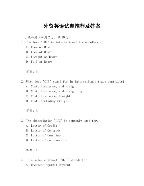
外贸英语试题推荐及答案一、选择题（每题2分，共20分）1. The term "FOB" in international trade refers to:A. Free on BoardB. Free of BoardC. Freight on BoardD. Full of Board答案：A2. What does "CIF" stand for in international trade contracts?A. Cost, Insurance, and FreightB. Cost, Insurance, and FreightingC. Cost, Insurance, FreightD. Cost, Including Freight答案：A3. The abbreviation "L/C" is commonly used for:A. Letter of CreditB. Letter of ContractC. Letter of CommitmentD. Letter of Confirmation答案：A4. In a sales contract, "D/P" stands for:A. Document against PaymentB. Direct PaymentC. Discounted PaymentD. Due Payment答案：A5. The term "T/T" in international trade transactions usually means:A. Transfer of TitleB. Transfer of TradeC. Telegraphic TransferD. Trade Transfer答案：C6. Which of the following is not a type of international trade document?A. Commercial InvoiceB. Bill of LadingC. Certificate of OriginD. Passport答案：D7. The term "EXW" in international trade is known as:A. Ex WorksB. Ex WarehouseC. Exclusive WorksD. Export Works答案：A8. "CIP" in international trade is short for:A. Carriage and Insurance Paid toB. Carriage in ProgressC. Cost, Insurance, and PaymentD. Cost, Including Payment答案：A9. What does "FCA" stand for in international trade?A. Free CarrierB. Full Container atC. Freight Carrier AgreementD. Forwarding Contract Agreement答案：A10. The term "D/A" in international trade usually refers to:A. Document against AcceptanceB. Direct AcceptanceC. Discounted AcceptanceD. Due Acceptance答案：A二、填空题（每题1分，共10分）11. The most common method of payment in international trade is ______.答案：Letter of Credit (L/C)12. When a seller offers goods "FOB", the risk passes to thebuyer when the goods pass over the ______.答案：ship's rail13. "CIF" includes the cost of the goods, ______, and insurance.答案：freight14. A ______ is a document that provides evidence of the origin of goods.答案：Certificate of Origin15. "T/T" can be used for both international and domestic payments and is quick and convenient.答案：Telegraphic Transfer16. "D/P" requires the buyer to pay for the goods before receiving the ______.答案：documents17. "EXW" means that the seller makes the goods available to the buyer at their ______.答案：place of business18. "CIP" terms require the seller to arrange for ______ and insurance.答案：carriage19. "FCA" means that the seller fulfills their obligations when the goods are handed over to the ______.答案：first carrier20. "D/A" is a method of payment where the documents are released to the buyer upon ______ of the draft.答案：acceptance三、简答题（每题5分，共30分）21. Explain the difference between "FOB" and "CIF" terms in international trade.答案："FOB" (Free on Board) terms mean that the seller's responsibility ends when the goods are loaded onto the ship, and the buyer bears all costs and risks from that point. "CIF" (Cost, Insurance, and Freight) terms include theseller's responsibility for the cost of the goods, freight to the agreed destination, and insurance.22. What are the advantages and disadvantages of using a Letter of Credit (L/C) in international trade?答案：Advantages include security for both the buyer and seller, as payment is guaranteed by a bank. Disadvantages include additional costs for bank fees and potential delays due to the time needed for bank processing.23. Describe the process of a Documentary Collection (D/P) in international trade.答案：In a Documentary Collection, the seller's bank forwards shipping documents to the buyer's bank, which then presents them to the buyer for payment. Once payment。

关于合同谈判纪要的呈批件英文回答：Memorandum.To: Senior Management.From: [Your Name]Date: March 8, 2023。

Subject: Contract Negotiation Memorandum.Introduction.The purpose of this memorandum is to summarize the key points discussed and agreements reached during the recent contract negotiations with [Counterparty Name]. The negotiations covered a range of issues, including pricing, terms of payment, delivery schedule, and dispute resolution.Negotiation Highlights.Pricing: We were able to negotiate a favorable price point that aligns with our budget and business objectives.Terms of Payment: We agreed to a payment schedule that provides flexibility and minimizes financial risk.Delivery Schedule: The delivery schedule was revised to accommodate our operational timelines and ensure timely completion of the project.Dispute Resolution: We established a clear dispute resolution process that promotes timely and efficient resolution of any potential conflicts.Key Agreements.The contract will be for a term of [duration] years.The contract will include a non-disclosure agreementto protect sensitive information.We will have the right to terminate the contract for cause in the event of material breach by the counterparty.The contract will be governed by the laws of [jurisdiction].Next Steps.We are currently working to finalize the contract language and will submit the final draft for your review and approval within the next [number] days. Once the contract is finalized and executed, we will proceed with the implementation of the agreement.Conclusion.The contract negotiations were conducted in a professional and collaborative manner. We believe that the agreements reached serve the best interests of both parties and lay the foundation for a successful partnership.中文回答：呈批件。

derivative securities analysis -回复Derivative securities analysis is a critical aspect of investment management, providing investors with insight into the potential risks and rewards associated with these complex financial instruments. This article aims to break down the concept of derivative securities analysis, exploring the steps and considerations taken in the evaluation process.Step 1: Understanding Derivative SecuritiesDerivative securities are financial contracts whose value is derived from an underlying asset. Common types of derivative securities include options, futures contracts, swaps, and forward contracts. An essential first step in derivative securities analysis is gaining a thorough understanding of these instruments and their characteristics.Step 2: Assessing Market ConditionsOnce the investor understands the basics of derivative securities, the next step involves assessing the market conditions. This includes analyzing factors such as interest rates, exchange rates, market volatility, and economic indicators that impact the underlying asset. Evaluating these conditions helps determine thepotential risks and opportunities associated with the derivative security.Step 3: Identifying Investment ObjectivesBefore delving into the analysis of derivative securities, investors need to identify their investment objectives. This can involve determining the desired risk tolerance, return expectations, and investment time horizon. Different derivative securities offer varying risk-reward profiles, so aligning investment objectives with the appropriate securities is crucial.Step 4: Analyzing the Derivative SecurityThe analysis of a derivative security typically involves conducting a variety of quantitative and qualitative evaluations. Quantitative analysis involves examining the mathematical models used to price the derivative security, such as options pricing models like the Black-Scholes model. This analysis helps assess the fair value of the derivative and potential profit or loss scenarios under different market conditions.Qualitative analysis, on the other hand, involves a deeper assessment of the factors that may impact the derivative security'svalue. This can include evaluating the creditworthiness of counterparties involved in the contract, the regulatory environment, and geopolitical risks.Step 5: Assessing Risk-Return CharacteristicsDerivative securities often come with various risks, including counterparty risk, liquidity risk, and market risk. Evaluating and understanding these risks is crucial in the analysis process. Investors must assess the risks associated with the derivative security and compare them to the potential returns. This analysis helps in determining if the risks are adequately compensated by the potential profits.Step 6: Monitoring and Re-evaluatingOnce an investment decision is made, it is essential to continuously monitor the derivative security's performance and market conditions. Market dynamics can change quickly, impacting the value and risks associated with the security. Regular monitoring and re-evaluation help ensure that investment objectives are continuously met and adjustments can be made if necessary.In conclusion, derivative securities analysis is a comprehensive process that involves understanding the instrument, assessing market conditions, identifying investment objectives, analyzing the security, assessing risk-return characteristics, and monitoring and re-evaluating. By following these steps and considering various factors, investors can make informed decisions about derivative securities and manage their risks effectively.。

随机利率下含信用风险的欧式期权的定价涂淑珍;黄婧;李时银【摘要】In this paper, we derive explicit pricing formula for vulnerable call options where the credit risk is handled in a hybrid model. We describe the process of default via a doubly stochastic Poisson process, and assume that the intensity processλof Poisson process follows an mean-reverting process. Moreover, the default intensity processλcorrelates with the underling asset and the value of the firm mutually. By applying equivalent martingale measure, we derive closed-form solutions of the pricing formulae within a general Gaussian interest rate framework.%采用混合定价方法给出了含信用风险的欧式期权在利率是随机情况下的模型。

采用公司定价模型中的补偿率，同时假定违约过程服从重Poisson随机过程。

其中违约过程的强度函数λ服从均值回复过程，且它与标的资产价格和公司价值相关。

运用等价鞅测度变换，给出了在随机利率框架下，含信用风险的期权价格的闭解。

【期刊名称】《龙岩学院学报》【年(卷),期】2015(000)005【总页数】8页(P18-25)【关键词】随机利率;重Poisson随机过程;信用风险;等价鞅测度【作者】涂淑珍;黄婧;李时银【作者单位】龙岩学院福建龙岩 364000;龙岩学院福建龙岩 364000;厦门大学福建厦门 361005【正文语种】中文【中图分类】O213数学·物理考虑信用风险的期权定价是当今金融研究的一个重要领域.对信用风险的定价模型主要有两种方法:结构模型(公司企业价值模型)和简化模型(强度函数模型).结构模型最早由Black和[1]和[2]提出,若期权到期时, 企业资产总值小于它的负债总额,则违约发生.这个框架内的主要问题是对公司价值以及公司资本结构的变化进行建模,相关研究成果有：Ammann [3], Johnson和[4],Klein和[5].而简化模型则是用一个外生的随机过程(通常用Poisson过程)来描述违约事件的发生,此方法主要要解决的问题是违约过程强度函数的确定,Jarrow和[6],Leung和[7], Guo和Jarrow 等[8]给出了该框架下的相关结论.本文采用混合定价模型来对含信用风险的欧式期权进行定价.用外生的重Poisson 过程来描述违约事件的发生,重Poisson随机过程的强度函数遵从均值回复过程.当违约发生时,采用公司价值模型中的补偿率,即期权多方到期时至多只能得到承诺支付的部分比率,该比率用来表示,其中VT,D分别表示公司资产价值和公司负债.同时,本文假定利率是随机的,服从高斯利率模型,且违约强度函数与标的资产价格和公式资产价值相关.在前人研究的基础上,先给出在远期风险中性测度下,标的资产以及公司资产价值的远期价格,通过等价鞅测度变换给出了含信用风险的欧式期权在远期测度下的定价方程及价格闭解.设(Ω,F,(Ft)t≥0,P) 为一完备的概率空间,(Ft)t≥0 为其上的对t递增的子σ域.假定对随机变量的所有叙述几乎处处成立,或几乎必然成立,P是风险中性概率,是右连续的,F0包含了当前时刻以及之前的所有信息.用(X):=EP(X|Ft)表示随机变量在t时刻以及t之前所有信息都已知情况下的条件期望.假定f(t,T)为远期利率,满足如下微分方程其中W为标准的布朗运动过程是Ft-适应的, 则瞬时利率为特殊的远期利率,满足r(t)=f(t,t),到期日为T的零息债券在t时的价格用远期利率来表示为P(t,T).同时,本文以零息债券价格P(t,T)为计价标准券,则价格变量it的远期价格可表示为.St表示股票的价格,Vt表示公司资产价值,则在风险中性概率测度P下,它们遵从如下几何布朗运动过程:其中r(t)遵从高斯利率模型,σS(t),σV(t) 是时间的确定性函数, 是P测度下的标准布朗运动过程.命题1[9] 在风险中性测度P下,到期日为T的零息债券价格为P(t,T)满足如下微分方程其中s.由命题1,可以得到如下命题.命题2 在风险中性测度P下,的微分形式分别如下设ξt是一重Poisson随机过程,违约强度函数为λt,满足均值回复过程[11],即其中α,m,σλ 为常数, 是标准的布朗运动过程.设期权的到期日为T,违约发生的时间为τ,τ=inf{t|ξt=1,0≤t≤T}表示过程{ξt}(t≥0)第一个事件的到达时间,则滤子,其中≤t),i=S,V,λ以及Ht=σ(I(τ≤s),s≤t).定义一个新的滤子，则τ的条件概率为[12]为简化计算,引入新的等价概率测度F,满足其中为违约风险的市场价格[13].命题3 SF,VF在新测度F下遵循的过程分别为:其中βi(t,T)=σi(t)+σ'(t,T),i=S,V是有界的和时间的确定性的函数.是F测度下的标准布朗运动.命题4[13] λ(t)在新测度F下遵循的过程为由Ito随机微分方程的知识[10],SF,VF和λ(t)的解为计算如下积分其中最后一步的计算应用了Fubini定理.为下文计算方便,定义令,其中i∈{S,V,λ}, 则SF(T,T),是ηS(t,T),ηV(t,T),ηλ(t,T)的函数,SF,VF和可以重新写成标准布朗运动) 的协方差矩阵为由于测度变换并不影响变量间的协方差,因此在F测度下,)的协方差矩阵仍为上式.由标准布朗运动的定义,有ηi(t,T),∀i∈{S,V,λ}遵从均值为0,方差为(t,T)的正态过程. 因此两两之间的协方差为对应的相关系数为为简化计算,作如下定义:由此,得到(ηS,ηV,ηλ)的相关系数矩阵记为从而联合分布函数为引理[14] 设某一风险收益在到期日T的收益为I(t≤τ≤T)δY+I(t>T)Y,若Y,δ是一G-可测的随机变量,τ,G,F的定义如1.2,令,则有进一步,如果Y是一FT-可测的随机变量,则有本文采用含信用风险的期权定价的混合模型.考虑含信用风险的期权具有双重风险:市场风险和违约风险,借助公司价值模型的补偿率,同时采用以强度为基础的的破产函数确定违约的发生.传统模型中假定违约过程是外生的,即违约强度与标的资产价格,企业价值不相关,但在现实经济社会中,违约强度λ与它们紧密相关.同时违约强度λ在实际中不太可能是确定性的,也不会任意变动,而是围绕其均值上下波动,故本文假定λ服从均值回复过程.同时,我们假定无风险利率是随机的,遵从高斯利率模型. 定理用重Poisson的随机过程{ξt}(t≥0)来控制违约过程,其中它的强度过程{λt}(t≥0)遵循均值回复过程,且违约强度过程{λt}(t≥0)与标的资产价格,企业价值的过程两两相关的情况下,承诺到期支付为XT=(ST-K)+,违约补偿率为cVTD的欧式期权在远期测度下的定价公式为(这里为了简化计算,初始时间为0 时刻)：其中的表达式如前所述.证明在高斯利率框架下,用远期中性测度推导含信用风险的期权的价格.含信用风险的期权在到期T时的价值为:其中第一部分为企业没有违约时的到期支付,第二部分为违约发生时的补偿支付.根据鞅定价原理,该期权在初始时刻的价值为这里用到P(T,T)=1.由引理,将(4)和I(τ>0)=1带入上式得,为方便起见,令EF[·]=EF[·|F0], 同时将上式拆分成四项X0=E1-E2+E3-E4,其中下面分别计算E1,E2,E3和E4.E1的计算.将式(1),(3)以及S(0,T)代入E1得由,故令,则有). 而对于SF(T,T)≥K,由(1),可以得到≥.通过简单的计算,可以得到下式: 定义x,令y=x,则其中n(·,·)是2维联合正态分布N(0,0,1,1;ρ)的密度函数,n(·),N(·)分别表示标准正态分布的密度函数和分布函数.第一个等号的成立运用N(b1)=1-N(-b1)这一结论.因此有其中类似E1的计算,同理可以得到E2的表达式如下：E3的计算.计算如下式子其中将式(1)和(2)以及S(0,T)代入得类似于(6)式的计算方法,得到对于的计算如下所示定义其中,则). 令,则有其中n(y1;Σ)表示三维正态分布N(0,0,0,1,1,1;Σ)的密度函数.综上,E3为类似E3的计算,同理可以得到E4的表达式如下：综合(6-9),即可得到式(5),证毕.本文采用混合定价模型,给出了考虑信用风险下,利率为随机利率时的欧式期权的价格.在传统模型的基础上,假定利率遵从高斯利率过程,违约强度函数遵从重Poisson 随机过程,且它与标的资产和企业价值都相关,这与传统模型相比更为接近实际情况,用此模型来定价含信用风险的欧式期权所得到的定价方程更为合理.本文建模过程中涉及到两种不同类型的不确定,一种不确定性来源于标的资产和公司资产价格,另一种则是来源于违约时间的不确定,而且这两种不确定存在相关关系.应用Nicole El Karoui给出的相关结论,通过计算最后给出了简化之后的期权价格如定理所示.可以从以下几个方面来扩展我们的研究,可以放宽假设,如公司的债务D可以考虑随机过程,同时可以把此方法用于含信用风险的多资产期权的定价问题,与传统方法相比,用该方法得到的解更为简化.【相关文献】[1] Black Fischer,Myron Scholes. The pricing of options and corporate liabilities[J]. The journal of political economy,1973,81(3): 637-654.[2] Merton Robert C. On the pricing of corporate debt: The risk structure of interestrates[J]. The Journal of Finance,1974,29(2): 449-470.[3] Ammann Manuel. Credit risk valuation: methods, models, and applications[M]. New York:Springer, 2001:194-200.[4] Johnson Herb, Rene Stulz. The pricing of options with default risk[J]. The journal of finance, 1987,42(2): 267-280.[5] Klein Peter, Michae lInglis. Pricing vulnerable European options when the option’s payoff can increase the risk of financial distress[J]. Journal of banking and finance, 2001,25(5):993-1012.[6] Jarrow Robert, Yu Fan. Counterparty risk and the pricing of defaultable securities[J]. The Journal of Finance, 2001,56(5):1765-1799.[7] Leung Kwai Sun, Kwok Yue Kuen. Counterparty risk for credit default swaps: Markov chain interacting intensities model with stochastic intensity[J]. Asia-Pacific Financial Markets, 2009,16(3): 169-181.[8] Guo Xin, Jarrow Robert, Yan Zeng. Modeling the recovery rate in a reduced form model[J]. Mathematical Finance, 2009,19(1): 73-97.[9] Duffie Darrell, Pan Jun, Kenneth Singleton. Transform analysis and asset pricing for affine jump-diffusions[J]. Econometrica, 2000,68(6): 1343-1376.[10] Kloeden Peter E.,Eckhard Platen. Numerical solution of stochastic differential equations[M]. New York: Springer,1992:253-266.[11] Fouque Jean-Pierre, George Papanicolaou, Ronnie Sircar. K. Mean-reverting stochastic volatility[J].International Journal of Theoretical and Applied Finance,2000,3(1):101-142.[12] 宋丽平,李时银. 违约风险定价模型的推广与应用[J].厦门大学学报:自然科学版,2005,44(5):616-620.[13] Blanchet Scalliet, Christophette, Nicole El Karoui, etc. Dynamic asset pricing theory with uncertain time-horizon[J]. Journal of Economic Dynamics and Control, 2005,29(10): 1737-1764.[14] Su Xiaonan, Wang Wensheng. Pricing options with credit risk in a reduced form model[J]. Journal of the Korean Statistical Society, 2012,41(4):437-444.。

No hedging Remained on book
Modern CRM Recent years Portfolio approach Scientific models Market value approach Mark to market or
model Credit derivative Integrated with
1. Introduction to Credit Risk Management
1.1 Definition and forms 1.2 Nature and Characteristics 1.3 Measurement 1.4 Management Strategies, and Instruments 1.5 History and Regulation 1.6 Traditional CRM vs. Modern CRM
Chapter 3 Credit Risk Management
1.Introduction to Credit Risk Management 2.Credit analysis and credit risk measuring: Traditional
approach 3.Credit analysis and credit risk measuring: Modern
5Cs
Character Capital Capacity Collateral Cycle or (Economic) Conditions + level of interest rates (nonlinear relationship
What cause credit risk?
Factors affecting the capability of borrowers: cash flow from different sources:

CFA衍生工具(Derivatives)考点解析对于很多想参加CFA考试的同学来说，对于CFA的考试内容还不是很了解。

我就为大家分享一下CFA考试的考试科目：1、道德与职业行为标准(Ethics and Professional Standards)2、定量分析(Quantitative)3、经济学(Economics)4、财务报表分析(Financial Statement Analysis)5、公司理财(Corporate Finance)6、权益投资(Equity Investments)7、固定收益投资(Fixed Income)8、衍生工具(Derivatives)9、其他类投资（Alternative Investments）10、投资组合管理(Portfolio Management)Derivatives（金融衍生品）很多CFA考生都认为一级里的Derivatives（金融衍生品）非常难，碰到这个章节就觉得十分头疼。

好在这个部分在考试中占比仅为5%，有些考生甚至采取了丢车保帅的做法。

提醒大家，不必对此产生畏难情绪。

CFA一级考试金融衍生品科目考试以前有一些计算，但现在以定性题目为主，要求考生能理解其中原由，难度有所下降。

随着国内逐渐开放衍生品市场，越来越需要有衍生品专业知识的人才。

这部分的衍生品主要介绍衍生品的一些基本知识，包括衍生品的种类及市场区分，4大类衍生品的基本定价原理，以及简单期权策略。

CFA一级考试的Derivatives（金融衍生品）具体的内容知识点包含1个study session，3个reading。

其中，Reading 57对衍生品市场进行了区别，并对4大类衍生品进行了基本定义；Reading 58讲衍生品的定价和估值的基本原理，并对4大类衍生品的基本定价做了介绍；Reading 59对期权做了进一步分析，介绍两种期权及两种期权策略的应用。

从CFA考试的重要度来看，Reading 58、Reading 59是最重要的，Reading 57其次，其他Reading重要性不大。

高三英语经济术语练习题50题1.The value of a currency is determined by many factors, including supply and demand. If the supply of a currency increases, its value is likely to _____.A.increaseB.decreaseC.remain unchangedD.fluctuate randomly答案：B。

解析：当一种货币的供应量增加时，根据供求关系，供大于求会导致其价值下降。

选项A 增加错误；选项C 保持不变错误；选项D 随机波动不准确，一般供应量增加价值倾向于下降。

2.In international trade, the exchange rate between two currencies can affect the price of imported and exported goods. If the exchange rate of a country's currency appreciates, the price of its exports is likely to _____.A.increaseB.decreaseC.remain unchangedD.depend on other factors答案：A。

解析：如果一个国家的货币汇率升值，那么其出口商品的价格会上升，因为同样的商品以本币计价不变，但换算成外币价格升高。

选项B 下降错误；选项C 保持不变错误；选项D 不准确，汇率升值出口价格通常会上升。

3.Different forms of money include cash and digital currency. Which of the following is an advantage of digital currency over cash?A.It is more widely accepted.B.It is easier to counterfeit.C.It offers more privacy.D.It is more convenient for online transactions.答案：D。

6级 – 呆坏账 被归为坏账 本金和利息的还款不大可能 银行可能会觉得必须变现抵押品才可 以还款 利息不能入账 (香港金管局90天逾期) 需要全额或部分拨备
50
信贷风险评级系统(续)
7级 – 损失 清算或结业的后阶段 需要全额拨备 收回款项的可能性很小 要进行相应的撇账
51
信贷风险评级系统(续)
41
按信贷等级分类的信贷组合
集团政策规定维持对FG1-3的92%信贷风险
42
信贷等级
43
信贷风险评级系统
7个信贷级别Vs5个信贷级别
对借款人评级Vs对单项借款评级
44
信贷风险评级系统(续)
1 级– 低风险 极佳的财务状况, 流动性,资本状况， 收入, 现金流, 管理和还款能力 借款由现金全额保证或是由 “Euromoney” 杂志评选出来的前100 家银行所签发的备用信 用证担保 借款人的穆迪评级是 Aaa 到>A3或是标准普尔评级是
AAA 到A
45
信贷风险评级系统(续)
2级 – 满意风险 令人满意的或是较好的财务状况, 流 动性,资本 状况, 收入, 现金流, 管理和 还款能力 Байду номын сангаас款人的穆迪评级是 Baa1 到Baa3或是标准普尔评 级是BBB+ 到BBB-
46
信贷风险评级系统(续)
3级 – 一般风险 收入或现金流有变差迹象 没有审计过的财务报表 账户交易记录或是还款纪录有问题 需要更频繁的监控 还款能力尚可 借款人的穆迪评级是 Ba1 到Ba3或是
标准普尔评级是BB+ 到BB-
47
信贷风险评级系统(续) 4 级– 关注级别 财务状况持续恶化 需要频繁的监控 还款能力尚可

巴塞尔协议第三版核心词汇I. 巴三六大目标一、更严格的资本定义（Increased Quality of Capital）：1．一级资本金包括：(1) 核心一级资本，(也叫普通股一级资本，common equity tier 1 capital)：只包括普通股（common equity）和留存收益（retained earning），巴三规定，少数股东权益（minority interest）、递延所得税(deferred tax)、对其他金融机构的投资(holdings in other financial institutions) 、商誉（goodwill）等不得计入核心一级资本。

(2) 其他一级资本：永久性优先股（non-cumulative preferred stock）等二、更高的资本充足要求（Increased Quantity of Capital）1．核心一级资本充足率(common equity tier 1 capital)：最低4.5%。

2．一级资本充足率：6%3．资本留存缓冲(capital conservation buffer)：最低2.5%，由普通股（扣除递延税项及其他项目）构成，用于危机期间（periods of stress）吸收损失，但是当该比率接近最低要求将影响奖金和红利发放(earning distributions）4．全部核心一级资本充足率(核心一级资本+资本留存缓冲)：最低7%5．总资本充足率（minimum total capital）：8%6．总资本充足率+资本留存缓冲最低要求：10.5%7．逆周期资本缓冲（counter-cyclical buffer）0—0.25%：在信贷增速过快(excessive credit growth)，导致系统范围内风险积聚时生效。

*** 巴三新资本要求：巴塞尔III将巴塞尔II中提出的一级资本、二级资本，并将一级资本重新划分为核心一级资本(主要包括普通股和留存收益)以及其他一级资本两大类。

• • • • It pays LIBOR + 0.8% to the outside lender It receives LIBOR (due to the Swap) It pays 5% (due to the Swap) Net effect: (Fixed) interest rate payment of 5.8%
• • • • It pays 5.2% to the outside lender It pays LIBOR (due to the Swap) It receives 5% (due to the Swap) Net effect: (Floating) interest rate payment of LIBOR + 0.2%.
A B
5%
Derivatives - Spring I 2016
3
Using the Swap to Transform a Liability (1)
• For company B the swap could be used to transform a floating-rate loan into a fixed-rate loan. Suppose that B borrowed $100 million at LIBOR + 80 basis point (0.8%). After B has entered into the swap, it really has 3 sets of cash flows:
LIBOR 5.2%
•
LIBOR
FI B
A
4.985%
5.015%LIBOR来自+ 0.8%•
•
In each case the FI has two separate contracts. If one company defaults the financial institution still has to honour its agreement with the other company. The 3/4 basis point spread compensates the financial institution for the default risk it is bearing and for its intermediation. In practise, financial institutions may not match counterparties and effectively stand ready to initiate these agreements (warehousing). One can view 4.985% and 5.015% as bid/ask rates quoted by the FI. The average value of these quoted bid/ask rates is generally called the swap rate.

ReferencesAcharya,V.,Engle,R.F.,Figlewski,S.,Lynch,A.W.and Subrahmanyam,M.G.(2009)Centralized Clearing for Credit Derivatives,in Restoring Financial Stability:How to Repair a Failed System ,Acharya,V .and Richardson,M.(eds),John Wiley &Sons Inc.Albanese,C.,D’Ippoliti,F.and Pietroniero,G.(2011)Margin Lending and Securitization:Regulators,Modelling and Technology,working paper.Altman,E.(1968)Financial Ratios,Discriminant Analysis and the Prediction of Corporate Bankruptcy.Journal of Finance ,23,589–609.Altman,E.(1989)Measuring Corporate Bond Mortality and Performance,Journal of Finance ,44(4,September),909–922.Altman,E.and Kishore,V.(1996)Almost Everything You Wanted to Know About Recoveries on Defaulted Bonds,Financial Analysts Journal ,Nov/Dec.Amdahl,G.(1967)Validity of the Single Processor Approach to Achieving Large-Scale Computing Capabilities,AFIPS Conference Proceedings,30,483–485.Andersen,L.and Piterbarg,V .(2010a)Interest Rate Modelling Volume 1:Foundations and Vanilla Models ,Atlantic Financial Press.Andersen,L.and Piterbarg,V.(2010b)Interest Rate Modelling Volume 2:Term Structure Models ,Atlantic Financial Press.Andersen,L.and Piterbarg,V .(2010c)Interest Rate Modelling Volume 3:Products and Risk Manage-ment ,Atlantic Financial Press.Andersen,L.,Sidenius,J.and Basu,S.(2003)All your hedges in one basket,Risk Magazine ,November.Arvanitis,A.and Gregory,J.(2001)Credit:The Complete Guide to Pricing,Hedging and Risk Man-agement ,Risk Books.Arvanitis,A.,Gregory,J.and Laurent,J.-P.(1999)Building Models for Credit Spreads,Journal of Derivatives ,6(3,Spring),27–43.Baird,D.G.(2001)Elements of Bankruptcy ,3rd edition,Foundation Press,New York,NY .Basel Committee on Banking Supervision (BCBS)(2004)An Explanatory Note on the Basel II IRB Risk Weight Functions,October,.Basel Committee on Banking Supervision (BCBS)(2005)The Application of Basel II to Trading Activities and the Treatment of Double Default,.Basel Committee on Banking Supervision (BCBS)(2006)International Convergence of Capital Measurement and Capital Standards,A Revised Framework –Comprehensive Version,June,.Basel Committee on Banking Supervision (BCBS)(2009)Strengthening the resilience of the banking sector,Consultative document,December,.Basel Committee on Banking Supervision (BCBS)(2010a)Basel III:A global regulatory framework for more resilient banks and banking systems,December (Revised June (2011),.Basel Committee on Banking Supervision (BCBS)(2010b)Basel III counterparty credit risk –Frequently asked questions,November,.Basel Committee on Banking Supervision (BCBS)(2011)Capitalisation of bank exposures to central counterparties,December,." / . ओ * # $ 7 9 3 ओ 3 ओ436ReferencesBasurto,M.S.and Singh,M.(2008)Counterparty Risk in the Over-the-Counter Derivatives Market, November.IMF Working Papers,1–19,Available at SSRN:/abstract¼1316726. Bates,D.and Craine,R.(1999)Valuing the Futures Market Clearinghouse’s Default Exposure during the1987Crash,Journal of Money,Credit&Banking,31(2,May),248–272.Bliss,R.R.and Kaufman,G.G.(2005)Derivatives and Systemic Risk:Netting,Collateral,and Closeout (May10th),FRB of Chicago Working Paper No.(2005)-03.Available at SSRN:/ abstract¼730648.Black,F.and Cox,J.(1976)Valuing Corporate Securities:Some Effects of Bond Indenture Provisions, Journal of Finance,31,351–67.Black,F.and Scholes,M.(1973)The Pricing of Options and Corporate Liabilities,Journal of Political Economy,81(3),637–654.Bluhm,C.,Overbeck,L.and Wagner,C.(2003)An Introduction to Credit Risk Modeling,Chapman and Hall.Brace,A.,Gatarek,D.and Musiela,M.(1997)The Market Model of Interest Rate Dynamics, Mathematical Finance,7(2),127–154.Brady,N.(1988)Report of the Presidential Task Force on Market Mechanisms,US Government Printing Office,Washington DC.Brigo,D.and Masetti,M.(2005a)Risk Neutral Pricing of Counterparty Risk,in Counterparty Credit Risk Modelling,Pykhtin,M.(ed.),Risk Books.Brigo,D.and Masetti,M.(2005b)A Formula for Interest Rate Swaps Valuation under Counterparty Risk in presence of Netting Agreements,www.damianobrigo.it.Brigo,D.and Morini,M.(2010)Dangers of Bilateral Counterparty Risk:the fundamental impact of closeout conventions,working paper.Brigo,D.and Morini,M.(2011)Closeout convention tensions,Risk,December,86–90.Brigo,D.,Chourdakis K.and Bakkar,I.(2008)Counterparty Risk Valuation for Energy Commodities Swaps:Impact of Volatilities and Correlation.Available at SSRN:/ abstract¼1150818.Burgard,C.and Kjaer,M.(2011a)Partial differential equation representations of derivatives with coun-terparty risk and funding costs,The Journal of Credit Risk,7(3),1–19.Burgard,C.and Kjaer,M.(2011b)In the balance,Risk,November,72–75.Burgard,C.and Kjaer,M.(2012)A Generalised CVA with Funding and Collateral,working paper. /abstract¼2027195.Canabarro,E.and Duffie,D.(2003)Measuring and Marking Counterparty Risk,in Asset/Liability Management for Financial Institutions,Tilman,L.(ed.),Institutional Investor Books. Canabarro,E.,Picoult,E.and Wilde,T.(2003)Analyzing counterparty risk,Risk,16(9),117–122. Cesari,G.,Aquilina,J.,Charpillon,N.,Filipovic,Z.,Lee,G.and Manda,I.(2009)Modelling,Pricing, and Hedging Counterparty Credit Exposure,Springer Finance.Collin-Dufresne,P.,Goldstein,R.S.and Martin,J.S.(2001)The Determinants of Credit Spread Changes,Journal of Finance,56,2177–2207.Cooper,I.A.and Mello,A.S.(1991)The default risk of swaps,Journal of Finance,46,597–620. Das,S.(2008)The Credit Default Swap(CDS)Market–Will It Unravel?,February2nd,http:// /Article3.1018þM583ca062a10.0.html.Das,S.and Sundaram,R.(1999)Of smiles and smirks,a term structure perspective,Journal of Finan-cial and Quantitative Analysis,34,211–239.De Prisco,B.and Rosen,D.(2005)Modelling Stochastic Counterparty Credit Exposures for Deriva-tives Portfolios,in Counterparty Credit Risk Modelling,Pykhtin,M.(ed.),Risk Books. Downing,C.,Underwood,S.and Xing,Y.(2005)Is liquidity risk priced in the corporate bond market?, Working paper,Rice University.Duffee,G.(1998)The Relation Between Treasury Yields and Corporate Bond Yield Spreads,The Journal of Finance,LIII(6,December).Duffee,G.R.(1996a)Idiosyncratic Variation of Treasury Bill Yields,Journal of Finance,51,527–551.References437 Duffee,G.R.(1996b)On measuring credit risks of derivative instruments,Journal of Banking and Finance,20(5),805–833.Duffie,D.(1999)Credit Swap Valuation,Financial Analysts Journal,January-February,73–87.Duffie,D.(2011)On the clearing of foreign exchange derivatives,working paper.Duffie,D.and Huang,M.(1996)Swap rates and credit quality,Journal of Finance,51,921–950.Duffie,D.and Singleton,K.J.(2003)Credit Risk:Pricing,Measurement,and Management,Princeton University Press.Duffie,D.and Zhu,H.(2009)Does a Central Clearing Counterparty Reduce Counterparty Risk?, working paper.Edwards F.R.and Morrison,E.R.(2005)Derivatives and the Bankruptcy Code:Why the Special Treatment?,Yale Journal on Regulation,22,91–122.Ehlers,P.and Sch€o nbucher,P.(2006)The Influence of FX Risk on Credit Spreads,working paper. Engelmann,B.and Rauhmeier,R.(eds)(2006)The Basel II Risk Parameters:Estimation,Validation, and Stress Testing,Springer.Figlewski,S.(1984)Margins and Market Integrity:Margin Setting for Stock Index Futures and Options,Journal of Futures Markets,13(4),389–408.Financial Times(2008)Banks face$10bn monolines charges,June10th.Finger,C.(1999)Conditional Approaches for CreditMetrics Portfolio Distributions,CreditMetrics Monitor,April.Finger,C.(2000)Towards a better understanding of wrong-way credit exposure,RiskMetrics working paper number99-05,February.Finger,C.,Finkelstein,V.,Pan,G.,Lardy,J.-P.and Tiemey,J.(2002)CreditGrades technical document. RiskMetrics Group.Fitzpatrick,K.(2002)Spotlight on counterparty risk,International Financial Review,99,November 30th.Fleck,M.and Schmidt,A.(2005)Analysis of Basel II Treatment of Counterparty Risk,in Counter-party Credit Risk Modelling,Pykhtin,M.(ed.),Risk Books.Fons,J.S.(1987)The Default Premium and Corporate Bond Experience,Journal of Finance,42 (1March),81–97.Garcia-Cespedes,J.C.,de Juan Herrero,J.A.,Rosen,D.and Saunders,D.(2010)Effective Modelling of Wrong-Way Risk,CCR Capital and Alpha in Basel II,Journal of Risk Model Validation,4(1),71–98. Garcia-Cespedes,J.C.,Keinin,A.,de Juan Herrero,J.A.and Rosen,D.(2006)A Simple Multi-Factor ‘Factor Adjustment’for Credit Capital Diversification,Special issue on Risk Concentrations in Credit Portfolios(Gordy,M.ed.)Journal of Credit Risk,Fall.Gemen,H.(2005)Commodities and commodity derivatives,John Wiley&Sons Ltd.Geman,H.and Nguyen,V.N.(2005)Soy bean inventory and forward curve dynamics,Management science,51(7,July),1076–1091.Gemmill,G.(1994)Margins and the Safety of Clearing Houses,Journal of Banking and Finance,18 (5),979–996.Ghosh,A.,Rennison,G.,Soulier,A.,Sharma,P.and Malinowska,M.(2008)Counterparty risk in credit markets,Barclays Capital Research Report.Gibson,M.S.(2005)Measuring counterparty credit risk exposure to a margined counterparty,in Coun-terparty Credit Risk Modelling,Pykhtin,M.(ed),Risk Books.Giesecke,K.,Longstaff,F.A.,Schaefer,S.and Strebulaev,I.(2010)Corporate Bond Default Risk: A150ÀYear Perspective,NBER Working Paper No.15848,March.Glasserman,P.and Li,J.(2005)Importance Sampling for Portfolio Credit Risk,Management Science, 51(11,November),1643–1656.Glasserman,P.and Yu,B.(2002)Pricing American options by simulation:regression now or regression later?,in Monte Carlo and Quasi-Monte Carlo Methods,Niederreiter,H.(ed),Springer.Gordy,M.(2002)Saddlepoint approximation of credit riskþ,Journal of Banking and Finance,26, 1335–1353.438ReferencesGordy,M.(2004)Granularity Adjustment in Portfolio Credit Risk Management,in Risk Measures for the21st Century,Szeg€o,G.P.(ed.),John Wiley&Sons.Gordy,M.and Howells,B.(2006)Procyclicality in Basel II:can we treat the disease without killing the patient?,Journal of Financial Intermediation,15,395–417.Gordy,M.and Juneja,S.(2008)Nested Simulation in Portfolio Risk Measurement,working paper. Gregory,J.(2008a)A trick of the credit tail,Risk,March,88–92.Gregory,J.(2008b)A free lunch and the credit crunch,Risk,August,74–77.Gregory,J.(2009a)Being two faced over counterparty credit risk,Risk,22(2),86–90.Gregory,J.(2009b)Counterparty credit risk:the new challenge for globalfinancial markets,John Wiley and Sons.Gregory,J.(2010)Counterparty casino:The need to address a systemic risk,European Policy Forum working paper.www.epfl.Gregory J.(2011)Counterparty risk in credit derivative contracts,in,The Oxford Handbook of Credit Derivatives,Lipton,A.and Rennie,A.(eds),Oxford University Press.Gregory,J.and German,I.(2012)Closing out DV A,working paper.Gregory,J.and Laurent,J.-P.(2003)I will survive,Risk,June,103–107.Gregory,J.and Laurent,J.-P.(2004)In the core of correlation,Risk,October87–91.Gupton,G.M.,Finger C.C.and Bhatia,M.(1997)CreditMetrics Technical Document,Morgan Guaranty Trust Company,New York.Hamilton,D.T.,Gupton,G.M.and Berthault,A.(2001)Default and Recovery Rates of Corporate Bond Issuers:(2000),Moody’s Investors Service,February.Hardouvelis,G.and Kim,D.(1995)Margin Requirements:Price Fluctuations,and Market Participa-tion in Metal Futures,Journal of Money,Credit and Banking,27(3),659–671.Hartzmark,M.(1986)The Effects of Changing Margin Levels on Futures Market Activity,the Compo-sition of Traders in the Market,and Price Performance,Journal of Business,59(2),S147–S180. Hille,C.T.,Ring J.and Shimanmoto,H.(2005)Modelling Counterparty Credit Exposure for Credit Default Swaps,in Counterparty Credit Risk Modelling,Pykhtin,M.(ed.),Risk Books.Hills,B.,Rule,D.,Parkinson,S.and Young,C.(1999)Central Counterparty Clearing Houses and Financial Stability,Bank of England Financial Stability Review,June,22–133.Hughston,L.P.and Turnbull,S.M.(2001)Credit risk:constructing the basic building block,Economic Notes,30(2),257–279.Hull,J.(2010)OTC Derivatives and Central Clearing:Can All Transactions Be Cleared?,working paper,April.Hull,J.and White,A.(1990)Pricing interest-rate derivative securities,The Review of Financial Stud-ies,3(4),573–592.Hull,J.and White,A.(1999)Pricing interest rate derivative securities,Review of Financial Studies, 3(4),573–92.Hull,J.and White,A.(2004)Valuation of a CDO and an nth to Default CDS without Monte Carlo Simulation,Working paper,September.Hull,J.and White,A.(2011)CVA and Wrong Way Risk,Working Paper,University of Toronto. Hull,J.,Predescu,M.and White,A.(2004)The Relationship Between Credit Default Swap Spreads, Bond Yields,and Credit Rating Announcements,Journal of Banking&Finance,28(11November), 2789–2811.Hull,J.,Predescu,M.and White,A.(2005a)Bond Prices,Default Probabilities and Risk Premiums, Journal of Credit Risk,1(2Spring),53–60.Hull,J.,Predescu,M.and White,A.(2005b)The valuation of correlation-dependent credit derivatives using a structural model,Journal of Credit Risk,6(3),99–132.Hull,J.,Predescu,M.and White,A,(2005c)The Valuation of Correlation-Dependent Credit Derivatives Using a Structural Model.Available at SSRN:/abstract¼686481. International Swaps and Derivatives Association(ISDA)(2009)ISDA close-out protocol,available at .References439 Jamshidian,F.and Zhu,Y.(1997)Scenario Simulation:Theory and methodology,Finance and Sto-chastics,1,43–67.Jarrow,R.A.and Turnbull,S.M.(1992)Drawing the analogy,Risk,5(10),63–70.Jarrow,R.A.and Turnbull,S.M.(1995)Pricing options onfinancial securities subject to default risk, Journal of Finance,50,53–86.Jarrow,R.and Turnbull,S.M.(1997)When swaps are dropped,Risk,10(5),70–75.Jarrow,R.A.and Yu,F.(2001)Counterparty risk and the pricing of defaultable securities,Journal of Finance,56,1765–1799.Johnson,H.and Stulz,R.(1987)The pricing of options with default risk,Journal of Finance,42, 267–280.Jorion,P.(2007)Value-at-Risk:The new benchmark for managingfinancial risk,3rd edition, McGraw-Hill.Kealhofer,S.(1995)Managing Default Risk in Derivative Portfolios,in Derivative Credit Risk: Advances in Measurement and Management,Jameson,R.(ed.),Renaissance Risk Publications. Kealhofer,S.(2003)Quantifying credit risk I:Default prediction,Financial Analysts Journal,January/ February,30–44.Kealhofer,S.and Kurbat,M.(2002)The Default Prediction Power of the Merton Approach,Relative to Debt Ratings and Accounting Variables,KMV LLC,Mimeo.KMV Corporation(1993)Portfolio management of default risk,San Francisco:KMV Corporation. Kenyon,C.(2010)Completing CVA and Liquidity:Firm-level positions and collateralized trades, working paper,.Kolb,R.W.and Overdahl,J.A.(2006)Understanding Futures Markets,Wiley-Blackwell. Kroszner,R.(1999)Can the Financial Markets Privately Regulate Risk?The Development of Deriva-tives Clearing Houses and Recent Over-the-Counter Innovations,Journal of Money,Credit,and Banking,August,569–618.Laurent,J.-P.and Gregory,J.(2005)Basket Default Swaps,CDOs and Factor Copulas,Journal of Risk, 7(4),103–122.Leland,H.(1994)Corporate Debt Value,Bond Covenants,and Optimal Capital Structure,Journal of Finance,49,1213–1252.Levy,A.and Levin,R.(1999)Wrong-way exposure,Risk,July.Li,D.X.(1998)Constructing a credit curve,Credit Risk:A RISK special report,November,40–44. Li,D.X.(2000)On Default Correlation:A Copula Function Approach,Journal of Fixed Income, 9(4March),43–54.Lomibao,D.and Zhu,S.(2005)A Conditional Valuation Approach for Path-Dependent Instruments,in Counterparty Credit Risk Modelling,Pykhtin,M.(ed),Risk Books.Longstaff,F.A.and Schwartz,S.E.(1995)A Simple Approach to Valuing Risky Fixed and Floating Rate Debt,The Journal of Finance,L(3July).Longstaff,F.A.and Schwarz,S.E.(2001)Valuing American options by simulation:A simple least squares approach,The review offinancial studies,14(1),113–147.Martin,R.,Thompson,K.and Browne,C.(2001)Taking to the saddle,Risk,June,91–94.Mashal,R.and Naldi,M.(2005)Pricing multiname default swaps with counterparty risk,Journal of Fixed Income,14(4),3–16.Matthews,R.A.J.(1995)Tumbling Toast,Murphy’s Law and the Fundamental Constants,European Journal of Physics,16,172–176.McKenzie,D.(2006)An Engine,Not a Camera:How Financial Models Shape Markets,MIT Press. Meese,R.and Rogoff,K.(1983)Empirical Exchange Rate Models of the Seventies,Journal of Inter-national Economics,14,3–24.Mercurio,F.(2010)A LIBOR Market Model with Stochastic Basis,available at SSRN:/ abstract¼1583081.Merton,R.C.(1974)On the Pricing of Corporate Debt:The Risk Structure of Interest Rates,Journal of Finance,29,449–70.440ReferencesMilne,A.(2012)Central Counterparty Clearing and the management of Systemic Default Risk, working paper,Loughborough University School of Business and Economics.Moody’s Investors Service(2007)Corporate Default and Recovery Rates:1920-(2006),Moody’s Special Report,New York,February.Morini,M.and Prampolini,A.(2010)Risky Funding:A unified framework for counterparty and liquidity charges,working paper./abstract¼1669930.O’Kane, D.(2007)Approximating Independent Loss Distributions with an Adjusted Binomial Distribution,EDHEC working paper.O’Kane,D.(2008)Modelling Single-name and Multi-name Credit Derivatives,John Wiley&Sons Ltd.Ong,M.K.(ed.)(2006)The Basel Handbook:A Guide for Financial Practitioners,2nd edition, Risk Books.Picoult,E.(2002)Quantifying the Risks of Trading,in Risk Management:Value at Risk and Beyond, Dempster,M.A.H.(ed.),Cambridge University Press.Picoult,E.(2005)Calculating and Hedging Exposure,Credit Value Adjustment and Economic Capital for Counterparty Credit Risk,in Counterparty Credit Risk Modelling,Pykhtin,M.(ed.),Risk Books. Pindyck,R.(2001)The dynamics of commodity spot and futures markets:A primer,Energy Journal, 22(3),1–29.Pirrong,C.(2000)A Theory of Financial Exchange Organization,Journal of Law and Economics,437. Pirrong,C.(2009)The Economics of Clearing in Derivatives Markets:Netting,Asymmetric Informa-tion,and the Sharing of Default Risks Through a Central Counterparty.Available at SSRN:http:// /abstract¼1340660.Pirrong,C.(2011)The Economics of Central Clearing:Theory and Practice,ISDA Discussion Papers Series Number One(May).Piterbarg,V.(2010)Funding beyond discounting:Collateral agreements and derivatives pricing,Risk, 2,97–102.Polizu,C.,Neilson F.L.and Khakee,N.(2006)Criteria for Rating Global Credit Derivative Product Companies,Standard&Poor’s working paper.Press,W.H.,Teukolsky,S.A.,Vetterling W.T.and Flannery,B.P.(2007)Numerical Recipes:The Art of Scientific Computing,3rd Edition,Cambridge University Press.Pugachevsky,D.(2005)Pricing counterparty risk in unfunded synthetic CDO tranches,in Counter-party Credit Risk Modelling,Pykhtin,M.(ed.),Risk Books.Pykhtin,M.(2003)Unexpected recovery risk,Risk,16(8),74–78.Pykhtin,M.(2012)Model foundations of the Basel III standardised CV A charge,Risk,July,60–66. Pykhtin,M.and Sokol,A.(2012)If a Dealer Defaulted,Would Anybody Notice?,working paper. Pykhtin,M.and Zhu,S.(2007)A Guide to Modelling Counterparty Credit Risk,GARP Risk Review, July/August,16–22.Rebonato,R.(1998)Interest Rate Options Models,2nd edition,John Wiley and Sons,Ltd. Reimers,M.and Zerbs,M.(1999)A multi-factor statistical model for interest rates,Algo Research Quarterly,2(3),53–64.Remeza,A.(2007)Credit Derivative Product Companies Poised to Open for Business,Moody’s Inves-tor Services special report.Rosen,D.and Pykhtin,M.(2010)Pricing Counterparty Risk at the Trade Level and CVA Allocations, Journal of Credit Risk,6(Winter),3–38.Rosen,D.and Saunders,D.(2010)Measuring Capital Contributions of Systemic Factors in Credit Portfolios,Journal of Banking and Finance,34,336–349.Rowe,D.(1995)Aggregating Credit Exposures:The Primary Risk Source Approach,in Derivative Credit Risk,Jameson,R.(ed.),Risk Publications,13–21.Rowe,D.and Mulholland,M.(1999)Aggregating Market-driven Credit Exposures:A Multiple Risk Source Approach,in Derivative Credit Risk,2nd edition,Incisive Media,141–147.References441 Sarno,L.(2005)Viewpoint:Towards a Solution to the Puzzles in Exchange Rate Economics:Where do we Stand?,Canadian Journal of Economics,38,673–708.Sarno,L.and Taylor,M.P.(2002)The Economics of Exchange Rates,Cambridge University Press. Segoviano,M.A.and Singh,M.(2008)Counterparty Risk in the Over-the-Counter Derivative market, IMF working paper,November.Shadab,H.B.(2009)Guilty by Association?Regulating Credit Default Swaps,Entrepreneurial Busi-ness Law Journal,August19,forthcoming.Available at SSRN:/abstract¼1368026. Shelton,D.(2004)Back to Normal,Proxy Integration:A fast accurate method for CDO and CDO-squared pricing,Citigroup Structured Credit Research,August.Singh,M.(2010)Collateral,Netting and Systemic Risk in the OTC Derivatives Market,IMF working paper,November.Singh,M.and Aitken,J.(2009)Deleveraging after Lehman–Evidence from Reduced Rehypotheca-tion,March,IMF Working Papers,1–11,available at SSRN:/abstract¼1366171. Sokol,A.(2010)A Practical Guide to Monte Carlo CVA,in Lessons From the Crisis,Berd,A.(ed.), Risk Books.Sorensen,E.H.and Bollier,T.F.(1994)Pricing Swap Default Risk,Financial Analysts Journal,50 (3May/June),23–33.Soros,G.(2009)My three steps tofinancial reform,Financial Times,June17th.Standard&Poor’s(2007)Ratings Performance:2006Stability and Transition,New York,S&P,16th February.Standard&Poor’s(2008)Default,Transition,and Recovery:2008Annual Global Corporate Default Study and Rating Transitions,April2nd.Tang,Y.and Williams,A.(2010)Funding benefit and funding cost,in Counterparty Credit Risk, Canabarro,E.(ed.),Risk Books.Tavakoli,J.M.(2008)Structured Finance and Collateralized Debt Obligations:New Developments in Cash and Synthetic Securitization,John Wiley&Sons,Inc.Tennant,J.,Emery,K.and Cantor,R.(2008)Corporate one-to-five-year rating transition rates, Moody’s Investor Services Special Comment.Thompson,J.R.(2009)Counterparty Risk in Financial Contracts:Should the Insured Worry About the Insurer?,available at SSRN:/abstract¼1278084.Turnbull,S.(2005)The Pricing Implications of Counterparty Risk for Non-Linear Credit Products,in Counterparty Credit Risk Modelling,Pykhtin,M.(ed.),Risk Books.Tzani,R.and Chen,J.J.(2006)Credit Derivative Product Companies,Moody’s Investor Services, March.Vasicek,O.(1997)The Loan Loss Distribution,KMV Corporation.Vrins,F.and Gregory,J.(2011)Getting CV A up and running,Risk,October.Wilde,T.(2001)The regulatory capital treatment of credit risk arising from OTC derivatives exposures in the trading and the banking book,in ISDA’s response to the Basel Committee On Banking Supervision’s Consultation on The New Capital Accord,May(2001),Annex1.Wilde,T.(2005)Analytic Methods for Portfolio Counterparty Risk,in Counterparty Credit Risk Modelling,Pykhtin,M.(ed.),Risk Books.。

国际贸易英语试题及答案一、选择题（每题2分，共20分）1. What is the most common mode of international trade?A. BarterB. Cash on deliveryC. Letters of creditD. Countertrade2. Which of the following is not a type of documentary credit?A. Sight L/CB. Usance L/CC. Standby L/CD. Promissory note3. What does "FOB" stand for in international trade terms?A. Free on BoardB. Free of BoardC. Freight on BoardD. Freight or Board4. In a letter of credit transaction, who is responsible for the payment to the seller?A. The buyerB. The sellerC. The issuing bankD. The advising bank5. What is the meaning of "CIF" in international trade?A. Cost, Insurance, and FreightB. Cost, Insurance, and Freight to the PortC. Cost, Insurance, and Freight to the DestinationD. Cost, Insurance, and Freight to the Seller6. Which of the following is not a risk associated with international trade?A. Currency fluctuationB. Political instabilityC. Market demandD. Transportation delays7. What is the role of an export license in international trade?A. To authorize the export of goodsB. To guarantee the quality of goodsC. To provide insurance for the goodsD. To ensure the goods are not counterfeit8. What does "GSP" stand for?A. Generalized System of PreferencesB. Global System of PreferencesC. Government Sponsored ProgramD. Governmental Support Plan9. Which of the following is not a form of international trade agreement?A. Bilateral agreementB. Multilateral agreementC. Unilateral agreementD. Regional trade agreement10. What is the purpose of a bill of lading in international trade?A. To confirm the receipt of goodsB. To serve as a contract of carriageC. To provide insurance for the goodsD. To authorize the payment of goods二、填空题（每题1分，共10分）11. The term "DAP" in international trade refers to _________ (Delivered at Place).12. An _________ (International Chamber of Commerce) provides rules for international trade.13. The _________ (World Trade Organization) regulates international trade.14. A _________ (Letter of Credit) is a written commitment bya bank to pay a specified amount to the seller.15. The _________ (International Monetary Fund) provides financial assistance to member countries.16. The term "EXW" stands for _________ (Ex Works).17. The _________ (United Nations Conference on Trade and Development) promotes international trade.18. A _________ (Commercial Invoice) is a document issued by the seller to the buyer.19. The _________ (Harmonized Commodity Description and Coding System) is used for classifying goods for customs purposes.20. An _________ (Import License) is required to import certain types of goods into a country.三、简答题（每题5分，共30分）21. Explain the difference between a documentary collection and a documentary credit.22. What are the benefits of using a letter of credit in international trade?23. Describe the process of a typical international trade transaction involving a letter of credit.24. What are the main factors to consider when negotiating the terms of an international sales contract?四、案例分析题（每题15分，共30分）25. A company in China has agreed to sell goods to a buyer in the United States. The terms of the sale are FOB Shanghai. What are the responsibilities of the seller and the buyer under these terms?26. A buyer in Germany has received a shipment of goods froma seller in India. Upon inspection, the buyer finds that the goods are damaged. The terms of the sale were CIF Hamburg. What are the buyer's options and what should be the seller's response?五、论述题（每题10分，共10分）27. Discuss the impact of globalization on international trade and how it has changed the way businesses operate internationally.答案：一、选择题1-5 CADCA6-10 DABCA二、填空题11. Delivered at Place12. International Chamber of Commerce13. World Trade Organization14. Letter of Credit15. International Monetary Fund16. Ex Works17. United Nations Conference on Trade and Development18. Commercial Invoice19. Harmonized Commodity Description and Coding System20. Import License三、简答题21. A documentary collection involves the collection of payment for goods shipped, usually through a bank, while a documentary credit is a commitment by a bank to。

1. A box spread is a combination of a bull spread composed of two call options with strike pricesand and a bear spread composed of two put options with the same two strike prices.a)Describe the payoff from a box spread on the expiration date of the options.b)What would be a fair price for the box spread today? Define variables asnecessary.c)Under what circumstances might an investor choose to construct a box spread?d)What sort of investor do you think is most likely to invest in such an optioncombination, i.e. a hedger, speculator or arbitrageur? Explain your answer.2. Form a long butterfly spread using the three call options in the table below.C1X = $90 T = 180 daysC2X = $100T = 180 daysC3X = $110T = 180 daysPrice 16.3300 10.3000 6.0600DELTA 0.7860 0.6151 0.4365GAMMA 0.0138 0.0181 0.0187THETA -11.2054 -12.2607 -11.4208VEGA 20.4619 26.8416 27.6602RHO 30.7085 25.2515 18.5394a)What does it cost to establish the butterfly spread?b)Calculate each of the Greek measures for this butterfly spread position and explainhow each can be interpreted.c)How would you make this option portfolio delta neutral? What would be achieved bydoing so?d)Suppose that tomorrow the price of C1 falls to $12.18 while the prices of C2 and C3remain the same. Does this create an arbitrage opportunity? Explain.3.Consider a six month American put option on index futures where the current futures price is450, the exercise price is 450, the risk-free rate of interest is 7 percent per annum, thecontinuous dividend yield of the index is 3 percent, and the volatility of the index is 30percent per annum. The futures contract underlying the option matures in seven months.Using a three-step binomial tree, calculatea)the price of the American put option now,b)the delta of the option with respect to the futures price,c)the delta of the option with respect to the index level, andd)the price of the corresponding European put option on index futures.e)Apply the control variate technique to improve your estimate of the American optionprice and of the delta of the option with respect to the futures price.Note that the Black-Scholes price of the European put option is $36.704 and the delta with respect to the futures price given by Black-Scholes is –0.442.4. A financial institution trades swaps where 12 month LIBOR is exchanged for a fixed rateof interest. Payments are made once a year. The one-year swap rate (i.e., the rate thatwould be exchanged for 12 month LIBOR in a new one-year swap) is 6 percent. Similarlythe two-year swap rate is 6.5 percent.a)Use this swap data to calculate the one and two year LIBOR zero rates, expressingthe rates with continuous compounding.b)What is the value of an existing swap with a notional principal of $10 million thathas two years to go and is such that financial institution pays 7 percent and receives12 month LIBOR? Payments are made once a year.c)What is the value of a forward rate agreement where a rate of 8 percent will bereceived on a principal of $1 million for the period between one year and two years?Note: All rates given in this question are expressed with annual compounding.5.The term structure is flat at 5% per annum with continuous compounding. Sometime ago a financial institution entered into a 5-year swap with a principal of$100 million in which every year it pays 12-month LIBOR and receives 6%.The swap now has two years eight months to run. Four months ago 12-monthLIBOR was 4% (with annual compounding). What is the value of the swaptoday? What is the financial institution’s credit exposure on the swap?6.An American put option to sell a Swiss franc for USD has a strike price of 0.80and a time to maturity of 1 year. The volatility of the Swiss franc is 10%, theUSD interest rate is 6%, and the Swiss franc interest rate is 3% (both interestrates continuously compounded). The current exchange rate is 0.81. Use a threetime step tree to value the option.7. A European call option on a certain stock has a strike price of $30, a time tomaturity of one year and an implied volatility of 30%. A put option on the samestock has a strike price of $30, a time to maturity of one year and an impliedvolatility of 33%. What is the arbitrage opportunity open to a trader. Does theopportunity work only when the lognormal assumption underlying Black-Scholes holds. Explain the reasons for your answer carefully.8. A put option on the S&P 500 has an exercise price of 500 and a time to maturity ofone year. The risk free rate is 7% and the dividend yield on the index is 3%. The volatility of the index is 20% per annum and the current level of the index is 500.A financial institution has a short position in the option.a) Calculate the delta, gamma, and vega of the position. Explain how they canbe interpreted.b) How can the position be made delta neutral?c) Suppose that one week later the index has increased to 515. How can deltaneutrality be preserved?9.An interest rate swap with a principal of $100 million involves the exchange of 5%per annum (semiannually compounded) for 6-month LIBOR. The remaining life is 14 months. Interest is exchanged every six months. The 2 month, 8 monthand 14 month rates are 4.5%, 5%, and 5.4% with continuous compounding. Six-month LIBOR was 5.5% four months ago. What is the value of the swap? 10.The Deutschemark-Canadian dollar exchange rate is currently 1.0000. At the endof 6 months it will be either 1.1000 or 0.9000. What is the value of a 6 monthoption to sell one million Canadian dollars for 1.05 million deutschemarks.Verify that the answer given by risk neutral valuation is the same as that given by no-arbitrage arguments. Is the option the same as one to buy 1.05 milliondeutschemarks for 1 million Canadian dollars? Assume that risk-free interestrates in Canada and Germany are 8% and 6% per annum respectively.11.An American put futures option has a strike price of 0.55 and a time to maturity of1 year. The current futures price is 0.60. The volatility of the futures price is25% and the interest rate(continuously compounded) is 6% per annum. Use a four time step tree to value the option.12.Is it ever optimal to exercise early an American call option on a) the spot price ofgold, b) the spot price of copper, c) the futures price of gold, and d) the average price of gold measured between time zero and the current time. Explain youranswers.13.The future probability distribution of a stock price has a fatter right tail and thinnerleft tail than the lognormal distribution. Describe the effect of this on the prices of in-the-money and out-of-the-money calls and puts. What is the volatilitysmile that would be observed?14.A bank has just sold a call option on 500,000 shares of a stock. The strike price is40; the stock price is 40; the risk-free rate is 5%; the volatility is 30%; and thetime to maturity is 3 months.a) What position should the company take in the stock for delta neutrality?b) Suppose that the bank does set up a delta neutral position as soon as theoption has been sold and the stock price jumps to 42 within the first hour oftrading. What trade is necessary to maintain delta neutrality? Explain whetherthe bank has gained or lost money in this situation. (You do not need tocalculate the exact amount gained or lost.)c) Repeat part b) on the assumption that the stock jumps to 38 instead of 4215.A bank has sold a product that offers investors the total return (excludingdividends) on the Toronto 300 index over a one year period. The return is capped at 20%. If the index goes down the original investment of the investor is returned.a) What option position is equivalent to the productb) Write down the formulas you would use to value the product and explain indetail how you would decide whether it is a good deal to the investore a three step tree to value a three month American put option on wheat futures.The current futures price is is 380 cents, the strike price is 370 cents, the risk-free rate is 5% per annum, and the volatility is 25% per annum. Explaincarefully what happens if the investor exercises the option after two months.Suppose that the futures price at the time of exercise is 362 and the most recent settlement price is 360.17.a) A bank’s assets and liabilities both have a duration of 5 ye ars. Is the bankhedged against interest rate movements? Explain carefully any limitations of the hedging scheme it has chosen.b) Explain what is meant by basis risk in the situation where a company knowsit will be purchasing a certain asset in two months and uses a three-monthfutures contract to hedge its risk.18.a) Give an example of how a swap might be used by a portfolio manager.b) Explain the nature of the credit risks to a financial institution in a swapagreementANSWERS1.(a) The box spread pays off X2-X1 in all circumstances (b) It should be worththe present value of X2-X1 today, c) and d) An arbitrageur might invest in a box spread if it is mispriced in the market today.2.(a) 1.79 b) Greek letters are -0.0077, -0.0037, etc c) For delta neutrality we buy0.0077 of the underlying asset. Small changes in the price of the underlyingasset then have very little effect on the value of the whole portfolio d) Yes. We have a positive cash flow when we set up the butterfly spread today and a zero or positive cash in 180 days3.a) 40.13, b) -0.449, c) F0=S0e0.04*7/12 or S0=0.9769F0 so that delta with respect tothe index level is =0.439, d) 39.81, e) American option price becomes40.13+36.704-39.81=37.02. Delta becomes -0.449 +0.444-0.442=-0.4474.a) One year rate is5.827%, two-year rate is6.313%, b) -$91,239, c) $8,5045. 3.50. This is also the credit exposure.6.0.0217.Put is priced too high relative to call. Sell put and buy call. This worksregardless of whether the assumptions underlying Black-Scholes hold8.a) 0.371, -0.0038, -1.85, b) Sell 0.371 of index for each option sold, c) Deltachanges to 0.317 so 0.054 of index must be bought back9.$841,000 assuming floating is received.10.Assume that the exchange rate is DM per $. p is then 0.450 and the value of theoption is about 80,000 DM. Yes the two options are the same.11.0.03612.a) no b)yes c)yes d)yes13.This will lead to a smile where volatility increases with strike price. this is theopposite of what is usually observed.14.a) Delta of long position in one option is 0.563. Bank should buy 281,500 sharesb) Delta changes to 0.686. Bank should buy a further 61,500 shares. The bankhas a negative gamma and so is likely to have lost money from the big move, c) Delta changes to 0.427. The bank should sell 68,000 shares. It will have lost money in this situation as well15.Suppose that S0 is invested in the product where S0 is the index level today. Thevalue of the investment in one year is S0 plus the payoff from a bull spread. The bull spread is created from a long call option with strike price S0 and a short call option with strike price 1.2S0. the interest earned can be calculated byvaluing the options. This can be compared with other market opportunities. 16.Value is 15.14 cents. Total gain from exercise after 2 months is 8 cents. therewould be a 10 cent cash pay off and a short futures position worth -2 cents. 17.a) Limitations relate to possibility of non-parallel shifts in the term structure andthe possibility of large movements b) basis risk arises from the differencebetween spot and futures price in 2 months18.a) A swap could be used to change an asset earning a fixed rate of interest to oneearning a floating rate. b) credit risks arise from the possibility of a default when the swap has a positive value and the counterparty defaults.内容总结。

一、引言信用违约互换（CDS）是指交易双方达成的，约定在未来一定期限内，信用保护买方按照约定的标准和方式向信用保护卖方支付信用保护费用，由信用保护卖方就约定的一个或多个参考实体向信用保护买方提供信用风险保护的金融合约，属于一种合约类信用风险缓释工具。

CDS对我国金融市场的发展至关重要：一是CDS可通过与其他信用衍生品相互补足促进，推动整个信用衍生品市场的流动性，促进我国信用衍生品市场的发展；二是CDS有助于丰富我国银行间市场参与者的信用风险管理策略，促进信用风险在不同金融市场和经济领域的合理配置和分散，平滑信用风险对经济金融体系造成的波动，增强金融体系的抗风险能力；三是CDS有助于缓解我国中低评级企业发债难问题，提升企业融资效率。

目前，以民营企业为代表的中低评级发行人发债较为困考虑卖方违约风险的CDS定价研究于善丽（1.中国人民银行金融研究所博士后科研流动站，北京100800；2.银行间市场清算所股份有限公司，上海200002）摘要：文章基于Copula和CIR模型，对考虑卖方违约风险的CDS定价研究进行了梳理，报告了同类研究中多将贴现率和违约强度设为固定常数，可能会导致定价结果与实际偏差较大的问题，并通过建立CIR动态变化方程拟合违约强度构建违约时间的分布函数，建立CIR随机利率变化方程确定无风险贴现函数予以解决，以尽可能确保考虑卖方违约风险的CDS定价结果准确性。

数值分析表明，文章计算的CDS定价结果较合理，且考虑卖方违约风险的CDS价格低于不考虑卖方违约风险的价格，这主要是由于当卖方违约风险增加时，买方愿意支付的CDS保费会降低，与实际相符。

最后，文章从CDS定价信息、标的范围和参与主体方面提出建议，以期助力完善我国的CDS定价机制。

关键词：信用违约互换定价；交易对手风险；CIR中图分类号：F830.59；F224；F830.91文献标识码：A文章编号：1004-292X（2020）10-0071-07CDS Pricing Considering Default Risk of SellerYU Shan-li(1.Postdoctoral Research Station,Financial Research Institute,People's Bank of China,Beijing100800,China;2.Shanghai Clearing House,Shanghai200002,China)Abstract:Based on Copula and CIR models,this paper combs the CDS pricing research considering the seller's default risk,and reports that the discount rate and default intensity are set as fixed constants in similar studies,which may lead to a large deviation between the pricing results and the actual value.By establishing CIR to fit the default intensity,the distribution function of default time is constructed,and using CIR to established the risk-free discount function,this paper ensures the accuracy of CDS pricing.Numerical analysis shows that the CDS pricing results calculated in this study are reasonable,and the CDS price considering the seller's default risk is lower than the price without considering the seller's default risk,this is mainly because when the seller's default risk increases,the CDS premium that the buyer is willing to pay will decrease,which is consistent with the actual situation.Finally,this paper puts forward suggestions from the aspects of CDS pricing information,target range and participants in order to help improve the CDS pricing mechanism in China.Key words:CDS pricing;Counterparty risk;CIR收稿日期：2020-06-27基金项目：国家自然科学基金重点项目（71731003，71431002）；国家自然科学基金面上项目（71873103，71971051，71971034）；国家自然科学基金青年科学基金项目（71901055，71903019）；中国博士后科学基金资助项目（2018M641578）；爱德力智能科技（厦门）有限公司智能风险管控模型与算法项目（2019-01）。