H.264码率控制方案jvt-g012
- 格式:doc
- 大小:693.00 KB
- 文档页数:34
有关码率控制的FAQ--------By Hychong1.码率控制中几个参数含义的理解在RC中经常会碰到这几个参数,InitialDelayOffset, Pm_X1,Pm_X2,Pm_rgQp[20],Pm_rgRp[20],UpperBound1, UpperBound2, LowerBound,谁能解释一下他们的含义啊,在程序里多次出现,就是搞不懂他们是用来干什么的,郁闷!你应该先好好学习一下JVT-H017r3,先熟悉理论,然后把代码跑起来跟踪JM 的RC 流程怎么走的,然后结合理论来理解就容易明白得多了。
UpperBound1, UpperBound2, LowerBound 就是JVT-H017r3 中的公式18、19Pm_rgQp、Pm_rgRp、Pm_X1、Pm_X2 的含义是:double Pm_rgQp[20]; //++ 参数值传递过程中的中间临时变量,可直接用m_rgQp 替换double Pm_rgRp[20]; //++ 参数值传递过程中的中间临时变量,可直接用m_rgRp 替换double Pm_X1; //++ 参数值传递过程中的中间临时变量,可直接用m_X1 替换double Pm_X2; //++ 参数值传递过程中的中间临时变量,可直接用m_X2 替换而m_rgQp、m_rgRp、m_X1、m_X2 的含义是:double m_rgQp[21]; //++ FIFO 队列用来存储各个基本单元的量化步长double m_rgRp[21]; //++ FIFO 队列用来存储各个基本单元编码完成后的二次方程左边项double m_X1; //++ 二次模型第一个系数double m_X2; //++ 二次模型第二个系数FIFO 队列则是指计算二次模型参数时候的样本候选队列。
这些思想都是来源于“Scalable Rate Control for MPEG-4 Video”这篇文章,看了这篇文章你就明白了。
一种视频编解码技术码率控制算法的改进
罗圣敏
【期刊名称】《计算机仿真》
【年(卷),期】2010(027)005
【摘要】H.264标准是最新的视频编码国际标准.与以前的视频压缩标准相
比,H.264标准的编码可以实现高质量、低比特率的编码效果.但它的码率控制算法JVT-G017在帧级码率控制上存在不足,平均分配目标比特,线性预测目标平均绝对误差值(MAD),这导致了计算复杂度大和峰值信噪比低.对此,在JVT-G017算法基础上,对其画面组(COP)层、帧层和基本单元层码率控制算法进行了优化改进,改进了分配目标比特数、初始量化参数(QP)和平均绝对误差值的计算方法.实验结果表明,与JVT-H017算法相比,改进算法可以更精确地分配目标比特和控制码率,并能获得较高的峰值信噪比(PSNR).
【总页数】4页(P359-362)
【作者】罗圣敏
【作者单位】清远职业技术学院,广东,清远,511500;中山大学,广东,广州,510275【正文语种】中文
【中图分类】TN948
【相关文献】
1.一种用于极低码率视频编码的码率控制算法 [J], 李甬;王洪玉;李宏东;李洁冰
2.改进的帧级视频编码码率控制算法 [J], 范桂真;杨静;王超
3.一种对H.264视频编码码率控制算法的改进 [J], 周明朗;李征
4.一种对H.264视频编码码率控制算法的改进 [J], 周明朗;李征
5.基于H.264标准的视频码率控制算法的改进 [J], 覃焕昌;
因版权原因,仅展示原文概要,查看原文内容请购买。
h.264的码率控制策略本文详细讨论了H.264编码标准的,与MPEG-2的TM5模型进行了比较;并对JVT-G012提出的流量往返控制模型进行了探讨;最后对H.264码率控制提出了一些改进意见。
关键词:H.264 码率控制VBR CBR一、引言到目前为止,视频编码标准通常采用去除时空域相关性的帧内/帧间预测、离散余弦变换量化和熵编码技术,以达到较高的编码效率。
对视频通信而言,由于通信信道带宽有限,需对视频编码码率进行控制,来保证编码码流的顺利传输和信道带宽的充分利用。
针对不同的应用场合,学者们提出了多种码率控制(Rate Control)策略。
其中,实时编码码率控制方法主要有两种:用先前宏块编码产生的比特数来预测当前宏块编码产生比特数,或者通过视频编码率失真函数来预测当前宏块编码产生的比特数。
码率控制算法[1]就是动态调整编码器参数,得到目标比特数。
它为视频序列中的图像组GOP、图像或者子图像分配一定的比特。
现有的码率控制算法主要是通。
实际上,量化参数(QP)反映了空间细节压缩情况,如QP小,大部分的细节都会被保留;QP增大,一些细节丢失,码率降低,但图像失真加强和质量下降。
也就是说,QP和比特率成反比的关系,而且随着视频源复杂度的提高,这种反比关系会更明显。
码率控制有两种模式:VBR和CBR,即可变比特控制和固定比特控制。
VBR模式是一种开环处理,。
由于实际视频序列中的图像复杂度是不断变化的,细节多少、运动快慢等等,比特率也相应变化,不稳定。
CBR模式是一种闭环处理,。
它根据对源复杂度估计、解码缓冲的大小及网络带宽估计动态调整QP,得到符合要求的码率。
二、H.264码率控制结构作为新一代的视频压缩编码标准,H.264对多编码模式、编码参数自适应选择、上下文自适应熵编码、多参考帧的灵活选择、高精度预测、去方块滤波以及抗误码能力等方面进行了精雕细刻,采取了一系列切合实际的技术措施,大大提高了编码效率和网络自适应能力。
第36卷第5期2008年10月浙江工业大学学报J OURNAL OF ZH E J IAN G UN IV ERSIT Y OF TECHNOLO GYVol.36No.5Oct.2008收稿日期:2007212213作者简介:周志立(1979—),男,浙江平阳人.硕士研究生,主要研究方向为信号处理、视频压缩.基于H.264的码率控制的改进方法研究周志立1,阮秀凯2(1.浙江工业大学信息学院,浙江杭州310032;2.南京邮电大学,江苏南京210003)摘要:码率控制是H.264中的一个重要的组成部分,其目标是在特定的条件下调整编码后的码流来满足的实际需求.最佳的码率控制由合适的比特分配和精准的比特率控制所共同决定.首先阐述了H.264中的码率控制方法及其要解决的问题,然后对J V T 关于H.264中码率控制的几个重要提案进行了深入分析,在此基础上结合现阶段的一些研究成果讨论了H.264码率控制改进方法.关键词:H.264;码率控制;R 2D 模型;MAD 模型;比特率分配中图分类号:TN919.8 文献标识码:A 文章编号:100624303(2008)0520519204R esearch on the improvement method of rate control based on H.264ZHOU Zhi 2li 1,RUAN Xiu 2kai 2(1.School of Information Engineering ,Zhejiang University of Technology ,Hangzhou 310032,China ;2.Nanjing University of Post s and Telecommunications ,Nanjing 210003,China )Abstract :Rate cont rol is one of most important part in H.264.The goal of rate control is to satisfy t he real requirement s t hrough adjusting t he coded bit st ream under t he specific conditions.The best rate cont rol can be decided by t he appropriate allocation of bit s and p recision of t he bit rate cont rol.Firstly ,t he met hods of rate cont rol in H.264and t he p roblems which need to be solved are int roduced.Then several important resolutions about rate cont rol met hods in H.264propo sed by J V T are analyzed deeply.Based on t hese research result s ,some improved met hods of rate control in H.264are discussed.K ey w ords :H.264;rate co nt rol ;R 2D model ;MAD model ;allocation of bit s0 引 言H.264是联合视频专家组(Jiont Vedio Team ,J V T )制定的关于视频编码的新标准,它在吸取了以往标准的优点的同时又增加了自己的一些新特点,如统一视频编码层的符号编码,高精度、多模式的位估计,基于4×4的整数变换,以及分层的编码语法等.这使得H.264的算法具有很高的编码效率,在相同的重建图像质量下,能够比H.263节约50%左右的比特率.若没有码率控制任何视频编码都难以在实际中获得应用,因此,针对不同的标准和用途,这就使得作为视频编码的关键技术之一的码率控制技术成为目前研究的热点.事实上,由于H.264标准里仅规定了编解码器的码流结构而并没有规定编码的具体细节,这给码率控制的优化工作带来了极大的便利,同时由于H.264标准的主要精力集中在编码码流及解码方法上,而并没有很好地研究码率控制,这预示着H.264的码率控制部分有着潜在的较大提升空间的余地.码率控制任务就是通过调节量化参数,使图像序列的比特率尽可能地与目标比特率一致,同时在保证缓冲比特占有度稳定的前提下,尽量保证图像质量的稳定.考虑到H.264引入了率失真优化控制(Rate Distortion Optimization,RDO)进行模式选择,量化参数(Quantization Parameter,Q P)同时使用于率失真优化和码率控制之中,也就导致了著名的“鸡蛋”悖论:为了计算当前的Q P需要当前宏块的运动估计残差,而运动估计残差只有在率失真优化之后才能得到,如果用预测帧与当前帧的平均绝对误差(Meam Absolute Different,MAD)来表示运动估计残差,则上述的悖论可用可表达为:Q P→RDO→MAD→Q P.笔者首先对目前J V T关于H.264的三个重要提案作了必要的分析,然后在此基础上研究了现阶段部分学者所提出的改进方法,最后为H.264的码率控制的总结及对H.264码率控制的改进方法进行了展望.1 JVT重要提案的分析1.1 JVT2D030该提案主要分为以下几个步骤:(a)比特分配;(b)第一次RDO;(c)确定量化参数;(d)第二次RDO.显然,在J V T2D030中,解决“鸡蛋”悖论的方法是采用二次编码的方案,这样就极大地增加了编码的复杂度,这也是该方案难以应用于实时传输中的主要原因.J V T2D030中对于帧复杂度的估计与该帧类型有关,且不同类型的帧分别设有独立的虚拟缓存,这样就再度增加了它的编码复杂度.同时,由于它的率失真模型过于简单,这就难以得到的精确的码率控制.1.2 JVT2G012由于J V T2D030中的上述不足,J V T2G012就取代J V T2D030成为H.264的标准码率控制的方法.在J V T2G012中,通过利用了图像的时空的相关性取代二次编码来解决“鸡蛋”悖论,即用线性MAD模型来估计帧的复杂度,用M PEG24的二次R2D(Quadratic Rate Distortion)模型来计算量化参数,同时J V T2G012中提出了宏块单元的概念,其可以是帧、片或宏块.该提案的主要步骤如下:(a)目标比特分配(b)预测MAD(c)用二次R2D模型计算Q P(d)执行RDO.J V T2G012中目标比特率的分配方案是把剩余的比特数平均分配给未编码的帧,而没有根据具体帧的复杂度,MAD是作为帧的复杂度用来解决“鸡蛋”悖论的,它的值是根据已编码的帧通过线性预测得到,在得到目标比特数与MAD后,用二次R2D模型计算Q P,最后利用所得到的Q P进行RDO模式选择.然而,J V T2G012并没有充分利用图像的时空相关性:首先,在MAD线性预测模型上,它运用于所有的宏块预测,但是对于空间较远的宏块而言,其空间相关性就很小,这样预测所得到的数据就不准确.其次,R2D模型上,由于J V T2G012采用了文献[1]中的M PEG24Q2模型,采用线性回归分析进行参数更新,其数据是在最近的编码块中得到,只适用于同一帧[2],这样只能得到空间的相关性;这显然是不够的,因为在实际的编码中,没有空间相关性或者空间相关性较弱但时间相关性较强的经常发生.所以在预测得到的图像复杂度还不能充分反映图像的特征;而且,该方程只适用于MAD值较大的情况,当MAD值较小时,采用用此模型得到的效果就不够精确[3].1.3 JVT2O016J V T2O016继承J V T2G012的传统算法,针对的上述不足,J V T2O016把主要方向锁定为充分挖掘图像序列的时空相关性,侧重点放在RDO模型的改进上:(1)R2D模型:将J V T2G012中采用的二次R2 D模型在当前帧量化步长的中值点用泰勒级数展开,利用在同一帧中量化步长变化小的特点得到新的R2D模型.(2)失真模型:认为与图像内容一样,失真也存在时空相关性,所以相邻的宏块的失真分布是相似的.基于这种思想,有效了利用图像的时空相关性导出新的线性失真预测模型.(3)率失真优化模型:基于上述新的R2D模型和失真模型,利用拉格朗日优化算法得到一种新的率失真优化模型.2 码率控制的改进方法由于H.264采用了多种改进编码效率的技术,对于码率控制,针对不同的应用可以选择不同的技・25・浙江工业大学学报第36卷术,其码率控制模型的建立也应该结合实际应用做出调整.码率控制改进的目标主要有:提高输出码率控制精度使其能够最大程度的接近目标码率;提高编码后输出比特流的峰值信噪比(Peak Signal to Noise Ratio,PSN R),减少其波动;提高运算速度,使其能够在实时条件下能够得到应用.笔者主要从下面的三个方面讨论码率控制的改进并进行了详细分析:(1)改进目标比特率的分配.(2)为更好地解决“鸡蛋”悖论,改进MAD 模型.(3)改进R2D模型.2.1 分配目标比特率的改进上述提案中,目标比特率的分配仅由缓存占有度决定,并且将GO P中剩余的比特数平均分配给了该GO P中未编码的所有帧,这样如果缓存占有度较高时,新帧就会分配较少的比特数,这样很可能引起跳帧和信噪比下降,从而可能使一个视频序列的不一致性失真,最后引起视频的不连贯性,这在急剧变化或场景切换的情况下更加明显.而实际上由于序列的运动性,帧间的差异有时是很显著的,所以在进行帧级目标比特率估计时,需要考虑帧内帧间的复杂度,使得码率控制性能够得到提高,因此结合图像本身的复杂性来优化码率分配成为改进算法性能的一种有效方法.这类算法可利用图像时空相关性,以MAD,信号的能量,PSN R和图像的直方图等不同形式作为图像复杂性的度量参数,用于调整剩余比特的分配.基于这种思想,文献[4]提出按能量大小对宏块进行比特分配,最后指出这种方法能够得到较好编码效果,文献[5]则用差分序列直方图(Histogram of Diferential sequence,HOD)来表示图像的复杂度进行比特分配,且该文献指出HOD 能很好的反映图像的复杂度,并且具有较低的计算复杂度.这种方法的优点在于它不改变现有H.264码率控制算法的整体框架,对编码计算复杂度影响不大.2.2 MAD模型的改进J V T标准的码率控制中,引进MAD的概念是为了用MAD表示图像的复杂度,然后利用线性预测模型得到MAD的值,从而来解决“鸡蛋”悖论,但因为线性预测并没有充分利用图像时间空的相关性,所以它不能精确的控制码率.文献[6]提出用MAD radio来代替MAD的方法,其中MAD radio是在原来MAD线形预测的基础上除以已编帧的平均MAD得到,用所编帧的MAD平均值作为序列的复杂度,并指出MAD radio能很好的反映帧的运动激烈程度.MAD的预测也可参考H.264中的运动矢量的预测方法,假设E为当前宏块,A,B,C分别为E的左,上和右上方的三个相对应块,宏块E的运动矢量的预测值是通过A,B,C得到的,所以我们也可把这种方法用于MAD的预测,从而更加合理地利用图像时空的相关性.由于DC T系数也能很好地表示图像复杂度或运动激烈程度,如果DCT系数越大,就表示运动越激烈,反之,则表示运动越平缓.有此学者提出,有效比特位的概念,对于DCT系数Y,如果编码器的最小量化步长为X,其有效比特位定义为v ali dB it(Y)=0,i f y=0int(log2(abs(y/x)+1),i f y≠0同时验证了有效比特位与输出码率之间的相互关系:编码输出码率会随着有效比特位的增加而增加.还讨论了宏块有效比特位和编码输出码率之间的关系,提出了码率的预测模型,然后在此基础上建立了宏块级的码率控制算法.文献[7]提出了一种基于线性ρ域模型的码率控制算法.ρ的意义定义为:将一个宏块做D C T变换后的系数以量化步长X进行量化,得到的系数中“0”所占的比例,公式如下ρ(X)=∑|a|<Xp(a)该算法通过大量实验发现图像编码后的比特率与ρ可以近似认为服从线性关系,这样,码率控制问题就转变为如何确立Rate2ρ和ρ2Q P的关系.另外,衡量图像复杂度的标准有很多种,除了上面提到的参数外,运动矢量本身也部分体现了图像复杂度,一般情况下,运动矢量绝对值越大,图像变换速度越快,其运动也就更加剧烈,所以在研究图像复杂度方面,这也是一个有效地改进的方向.2.3 R2D模型的改进J V T标准算法采用的二次R2D模型是基于DCT系数拉普拉斯分布模型而建立的.然而,在低码率环境下,H.264码率失真不能很精确地吻合该模型.据此,文献[8]认为很多情况下用柯西分布来近似DC T系数的分布更为合理,该文献提出了一・125・第5期周志立,等:基于H.264的码率控制的改进方法研究种基于柯西分布的率失真模型,并简化得到如下近似形式以降低计算复杂度R(Q)≈aQαD(Q)≈bQβ其中a,b,α,β为常数,R,D,Q分别为码率,率失真和量化参数.J V T标准中,采用了二次R2D模型来计算Q P,而Q P的选择对性能的影响是至关重要的,如果Q P 选得太高则使得失真率过高,反之,如果选得Q P选得太低则输出的比特数就会急剧增加.大量的实验表明在Q P值基本在20-40之间,这时,Q P与R 之间的关系可近似地认为是线性的.此时,可以对R2D模型近似用一次模型来代替二次模型,这样就可大大地简化计算的复杂度,这种方法一般用于对失真度要求度不高但实时要求较为严格的场合.除上述的改进方法外,还可以在其它方面加以改进,比如在R2D模型上可根据特殊的应用对公式的细节加以修剪,从而简化它的计算复杂度,还可考虑从量化参数的选取及缓冲状态等方面考虑对码率控制的算法进行改进,还可考虑采用联合信源信道编码等,在低延时下可采用跳帧技术.3 结束语H.264具有很高的压缩效率,但这是以牺牲计算复杂度为代价的,因此,在实时应用的场合,它的应用得到了一定的限制.在保证准确码率控制的前提下,如何最大程度地降低计算的复杂度无疑是今后码率控制方法改进的热点.码率控制算法的改进点比较多,更多的结合图像序列的特征进行码率控制是很有潜力的一个方向,对于不同图像序列的运动特征及不同的应用,码率控制的方法也相应的有所不同,因此,建立一个各种序列各种场合都适应的控制模型是不切合实际的.参考文献:[1] TIHAO C,ZHAN G Y aqin.A new rate control scheme usingquadratic rate distortion model[J].IEEE T ransaction On CircuitsAnd Systems For Video T echnology,1997,2:2462250.[2] WU Yuan,L IN Shouxun,ZHAN G Y ongdong,et al.Optimumbit allocation and rate control for H.264/AVC[C].15t hMeeting,Busan,KR,2005:16222.[3] XU Jianfeng,HE Yun.A novel rate control for H.264[J].IEEET ransactions on Image processing.2004,23(5):8092812.[4] WAN G Ning,H E Yun.A new bitrate control strategy for H.264[J].IEEE Transactions on Signal Processing,2003,15(12):137021374.[5] L EE J,DICKINSON B W.Temporally adaptive motion inter2polation exploting temporal masking in visual perception[J].IEE Transactions on Image Processing,1994,3(5):5132526.[6] J IAN G Minqiang,YI Xiaoquan,L IN G Nam.Improved frame2layer rate control for H.264using MAD ratio[J].Circuit sand Systems ISCAS apos,2004,23(5):8132816.[7] SHINIH L P.Rate control using linear rate2ρmodel for H.264[J].signal Processing On Image Communication,2004,4:3142352.[8] YUCEL A,N EJ A T K.An analysis of t he DCT coefficent dis2tribution wit h t he H.264[J].IEEE International Conference,2004,17(5):1772180.(责任编辑:翁爱湘)・225・浙江工业大学学报第36卷。
基于运动检测的H.264码率控制的算法
李慧然;彭强;陈睿
【期刊名称】《计算机应用》
【年(卷),期】2008(28)2
【摘要】针对H.264/AVC 经典流控算法JVT-G012对运动剧烈图像流控效率的不足,提出了一种基于图像运动剧烈程度的流控算法.对运动剧烈的图像,在同一复杂度区域内,用前一帧实际编码码率与目标码率的差值调整当前帧目标码率,并且编码时利用最小率失真模式的原始帧和重建帧的SAD估计MAD值,根据二次模型估计量化参数优化拉格朗日参数.仿真试验证明与JVT-G012以及Jiang等对
H.264AVC的改进的码率控制算法相比,在运动剧烈或者场景切换时,虽然码率比JVT-G012略有增加但低于Jiang等的改进算法,并且变化剧烈的视频帧图像信噪比有明显的增加,平均信噪比也得到了提高.
【总页数】4页(P385-388)
【作者】李慧然;彭强;陈睿
【作者单位】西南交通大学,信息科学与技术学院,成都,610031;西南交通大学,信息科学与技术学院,成都,610031;中兴通讯股份有限公司,中心研究院,广东,深
圳,518057
【正文语种】中文
【中图分类】TP37
【相关文献】
1.基于人眼视觉系统的H.264/AVC码率控制算法 [J], 孙乐;戴明;陈晓露;王子辰;赵春蕾
2.一种基于视觉感知的H.264码率控制算法 [J], 田波;杨宜民;蔡述庭;
3.基于H.264编码域的显著运动检测算法 [J], 王靖雄;田翔;胡银丰
4.基于H.264 AVC的码率控制算法研究 [J], 李琳
5.一种基于运动检测的码率控制算法 [J], 刘振宇;周莉;陈杰
因版权原因,仅展示原文概要,查看原文内容请购买。
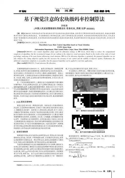
Science &Technology Vision 科技视界在视频编码标准H.264/AVC 中,通常以客观标准(如峰值信噪比,PSNR)来评价压缩后的视频质量,客观质量评定方法具有速度快、易实行的特点,但其结果往往不太符合人眼的主观视觉感受。
视觉心理学研究表明,人类视觉系统(HVS)对图像和视频的主观感知受到亮度、对比度、颜色、纹理、运动和位置等多种因素影响,并存在空间、时间和色彩的掩盖效应[1]。
在一个复杂的视觉场景中,人眼的注意力迅速被场景中感兴趣的区域所吸引,并优先处理这些信息,这个过程称为视觉注意。
对视觉注意机制的研究表明,人眼在观看视频图像时,视觉注意力往往不是均匀分布在整幅图像中,而是集中在其中的某些部分,对这些部分的图像失真也更加敏感[2]。
因此在视频编码过程中,对人眼注意力集中的区域分配较多的目标比特,以获得更好的视频质量,而对人眼处理优先级较低,不容易引起注意的区域分配较少的目标比特,提高视频编码效率。
1HVS 视觉注意特性视觉注意是HVS 的一种潜意识过程,同时也是人类最具体的认识过程,它受到两类因素影响:自顶向下(概念驱动)的因素和自底向上(刺激驱动)的因素[3]。
前者来自人类复杂的心理过程,受个人知识、兴趣爱好等因素影响,比如基于知识和经验的模式识别,它使人眼直接关注场景中某些对象的特征。
后者是指视频场景中与人眼光学属性和视网膜相关的因素,比如颜色、对比度、空间掩蔽、时间掩蔽和对象运动等。
目前视觉注意方面的研究,主要是通过建立自底向上的注意力分析模型来表示视觉内容,然而分析每种影响视觉注意因素的计算复杂度非常高,并不适合实时视频编码应用。
大量实验表明[4-5],视频场景中的对象运动和纹理区域是影响视觉注意力分布的最重要的因素,因此我们主要考虑这两方面因素优化目标比特分配。
2运动区域检测视频场景中的运动分为前景运动和背景运动,背景运动主要由摄像机的运动引起,如变焦、平移和旋转动作,以及场景光线变化;前景运动指视频中对象的运动。

一种H.264帧级码率控制改进算法
刘启;石志强
【期刊名称】《计算机仿真》
【年(卷),期】2008(025)005
【摘要】H.264是现在最新、最有前途的视频压缩标准.它的码率控制算法JVT-G012能获得良好的效果,但该算法在帧级码率控制上存在不足.在JVT-G012算法基础上,采取了一些帧级码率优化策略,用P帧亮度分量的平均绝对值差(MAD)比率来表示图像复杂度,同时根据编码图像复杂度和距离I帧的远近来合理有效的分配码率,增加了跳帧控制防止缓冲区发生上溢或者下溢,并且进行了场景切换检测.仿真采用Jm10.0,模拟了在恒定比特率(Constant Bit Rate,CBR)条件下,对算法和JVT-G012算法产生的编码质量进行对比.仿真结果表明,与JVT-G012算法相比,算法能使码率控制算法具有更高的效率、更有效地提高编码图像质量.
【总页数】4页(P105-108)
【作者】刘启;石志强
【作者单位】中国科学院研究生院,北京,100080;中国科学院软件研究所,北
京,100039
【正文语种】中文
【中图分类】TP391.41
【相关文献】
1.一种基于H.264/AVC宏块级改进的码率控制算法 [J], 金建;李小红;李寅
2.一种改进的H.264/AVC帧层码率控制算法 [J], 陈晓;刘海英
3.一种面向H.264标准的帧层码率控制算法改进 [J], 郭红英;蔡坚勇;涂钦;林潇;吴怡
4.一种H.264帧层码率控制的改进算法 [J], 段厚勇;汪同庆
5.一种改进的H.264帧层码率控制算法 [J], 吴军;胡建总;谢斌;王怡爽
因版权原因,仅展示原文概要,查看原文内容请购买。
针对H.264码率控制的初始量化参数选择算法0引言H.264/AVC是目前最通用的高性能视频编解码标准之一[1]。
码率控制作为视频编码中的一项重要技术,其目的是在满足带宽限制的前提下尽量提高解码端视频的质量[2]。
现有H.264码率控制提案包括JVT F086[3]、JVT G012[4]、JVT H017[5]。
目前H.264采用JVT H017提案所提算法[6-7],该算法中初始量化参数的选择与视频内容无关,影响码率控制性能。
针对这一问题,很多研究者提出了改进方案,文献[8-12]提出通过提取原始像素信息或预测信息表征视频内容特性来计算初始量化参数(QuantizationParameter,QP)的方法,文献[13]提出用神经网络来拟合初始QP的算法。
但这些算法的复杂度都很高,且不适用于IBBP编码结构。
本文详细分析了现有算法存在的问题,并通过实验发现像素平均比特率(bitsperpixel,bpp)与最优初始QP之间存在良好的幂指数关系,在此基础上提出一种有效预测初始QP算法,算法模型参数的计算被精心设计,算法复杂度很低。
3.2模型准确性验证使用H.264/AVC参考模型JM17.2[16],在多个目标比特率下,对不同内容特性序列使用所提模型预测得到初始QP。
图3所示预测初始QP与最优初始QP的比较结果。
4实验结果及分析为了验证提出算法的性能,使用H.264/AVC参考模型JM17.2,选取不同内容特性序列Akiyo、Silent、Paris、News、Football作为实验序列,编码前50帧,帧率30帧/s,开启码率控制,编码结构IPPP、IBBP。
表2、表3为改进算法与JVT H017算法率失真性能比较。
从表中可以看出,与JVT H017算法相比,本文改进算法在保证准确控制码率的前提下,峰值信噪比(PeakSignal to NoiseRatio,PSNR)有明显提高,ΔPSNR最大能提高1.1dB。
二、H.264标准的码率控制模块(rate control)规范描述H.264标准中码率控制方法的提案主要有三个:JVT-F086(2002)算法、JvT-G012(2003)算法和JVT-O016(2005)算法,后两种即通常所说的李氏提案和吴氏提案。
其JVT-F086可以看成是MPEG-2 TM5改进版本;JVT-G012算法用流量往返模型来分配每个基本单元目标比特数,并采用二次率失真函数计算量化参数后进行编码,而JVT-O016则继承了JVT-G012的传统算法,侧重于率失真优化RDO模型的改进,充分挖掘图像的时空相关性。
2.1 JVT-F086(2002)JVT-F086算法与MPEG-2的码率控制算法TM5类似,其工作流程同样由三步组成。
首先是目标比特分配,在图像编码前,估计出对下一帧图像编码所需要的比特数:接着是速率控制,通过一个虚拟缓存器,给每个宏块设定量化参数的参考值;最后是自适应量化,根据宏块的空间活动性来调整量化参数的参考值,以获得用于宏块的量化参数值。
JVT-F086算法结构如图2-1所示:图2-1 JVT-F086算法结构图在目标比特分配步骤中,首先对图像序列中的第一个I帧,P帧或B帧定义不同的总体复杂度的度量,具体可由下式得到:,具体可由下式得到:=115*bitrate/115=15*bitrate/115=5*bitrate/115得到总体复杂度的度量以后,再求得下一帧图像的目标比特数目,即,根据分配给该组图像(GOP)的总比特数R来计算。
如果当前图像GOP(INTRA帧)是第一个,那么R值更新如下:R=bitrate*(++1)/framerateN是GOP中图像的数目,和分别是当前GOP中未编码的P帧和B帧的数目,且R初始设定为0。
如果当前帧不是GOP中的第一个图像,如果图像序列中已编码比特数为nbits,那么R值更新如下:R- nbits→R计算出分配给下一帧的目标比特数后,步骤一将结果传递给步骤二,进行速率控制,速率控制步骤基于虚拟缓存器的概念,在编码宏j(j>=1)之前,虚拟缓存器饱和度基于图像类型来计算:=QP*10*bitrate/(31*framerate)=(QP+2)*10*bitrate/(31*framerate)=(QP+2)*10*bitrate/31这里,,,的值分别是对I,P,B帧型的虚拟缓存器的初始饱和度值。
JM参考软件采用G012的JVT自适应基本单元层码率控制算法1。
基础知识QP:Quantization Parameter量化参数RDO:Rate Distortion Optimization率失真优化MAD:Mean Absolute Difference绝对平均差值Basic Unit:基本单元Leaky Bucket Model:漏桶模型Linear Tracking Theory:线性跟踪理论Buffer Occupancy:缓冲占有率Buffer Fullness:缓冲充盈度Buffer Level:缓冲级别Quadratic Rate—Distortion Model:二次率失真模型VBR:Variable Bit Rate变比特率VBR:Constant Bit Rate恒定比特率HRD:Hypothetical Reference Decoder假想参考解码器Fluid Flow Traffic Model:流体传输模型GOP:Group of Pictures图像组1.1 蛋鸡悖论码率控制相关的宏块编码过程如下:码率控制→量化参数QP→率失真优化RDO→绝对平均差值MAD→编码问题:为了对宏块进行RDO,必须先用宏块的MAD值来确定宏块的QP值。
然而当前宏块的MAD值只有在RDO之后才可以获取,这样就产生了蛋鸡悖论。
解决办法:本文中提出了自适应基本单元层码率控制方案,提出基本单元和线性模型的概念.其中,基本单元可为一帧、一片或一个宏块。
而线性模型是用前一帧相同位置处的基本单元的MAD值来预测当前帧当前基本单元的MAD值,这样求MAD值就可以解决蛋鸡悖论.解决过程如下:采用漏桶模型和线性跟踪理论,根据已经确定的帧率、当前的缓冲占有率、目标缓冲级别和可获取的信道带宽来算出当前帧的目标码率。
剩余比特数则平均分配给当前帧中没有编码的基本单元,因为这些基本单元的MAD值还不知道.通过线性模型,可用前一帧相同位置处的基本单元的实际MAD值来预测出当前基本单元的MAD值.之后,用二次率失真模型来计算相应的QP值,从而用来对当前基本单元的每一宏块进行率失真优化.我们侧重考虑变比特率的情况,恒定比特率情况下也同样很适用.方案中还采用了一个虚拟缓冲来根据信道带宽的变化来调节编码过程。
视频编码线性码率控制模型任江涛;元辉;常义林;任光亮【摘要】为提高视频编码码率控制的性能,通过理论推导及实验验证提出了一种新的视频编码码率控制模型.通过该模型,编码器可以直接确定量化参数(Quantization Parameter, QP),而不必计算量化步长(Quantization Step, Qstep),进而避免了由Qstep确定QP 过程中的舍入误差,提高了码率控制的准确性.实验结果表明,与H.264/AVC采用的码率控制方法相比,提出的模型可使跳帧发生的概率更低,恢复视频的质量更稳定,实际码率与目标码率之间的偏差更小,同时,还能获得更高的峰值信噪比.【期刊名称】《电讯技术》【年(卷),期】2010(050)010【总页数】5页(P23-27)【关键词】视频编码;码率控制;率失真模型;量化参数;峰值信噪比【作者】任江涛;元辉;常义林;任光亮【作者单位】西安电子科技大学,ISN国家重点实验室,西安,710071;西安电子科技大学,ISN国家重点实验室,西安,710071;西安电子科技大学,ISN国家重点实验室,西安,710071;西安电子科技大学,ISN国家重点实验室,西安,710071【正文语种】中文【中图分类】TN919.81 引言视频压缩的最终目的是占用较少的资源,获得较高的视频质量。
实际应用中,考虑可用资源受限的条件下,为使接收端获得质量最好的恢复视频质量,码率控制成为视频编码器的重要组成部分[1]。
码率控制是指为编码器确定编码参数对视频进行编码,使得接收端恢复视频的质量在信道带宽、编码器缓冲区大小等受限的条件下尽可能高。
目前,H.264/AVC[2]的参考软件[3]将JVT-G012[4]和JVT-W042[5]作为其推荐使用的码率控制方案。
现有的码率控制机制普遍通过建立码率-量化步长(R-Qstep)模型[6-9]为编码器确定编码参数,比如JVT-G012和JVT-W042采用的二次模型[7]。
Joint Video Team (JVT) of ISO/IEC MPEG & ITU-T VCEG (ISO/IEC JTC1/SC29/WG11 and ITU-T SG16 Q.6)7th Meeting: Pattaya II ,Thailand, 7-14 March, 2003Document: JVT-G012 Filename: JVT-G012.docTitle: Adaptive Basic Unit Layer Rate Control for JVT Status: [Input Document to JVT]Purpose: [ Proposal]Author(s) or Contact(s): Zhengguo Li, Feng Pan, Keng PangLim, Genan Feng, Xiao Lin andSusanto RahardjaSignal Processing Program, Institutefor InfoComm Research21 Heng Mui Keng TerraceSingapore 119613Tel:Email:+65 6874 6874{ezgli,efpan,kplim,gnfeng,linxiao,rsusanto}@i2r.a-.sgSource: [Institute for InfoComm Research]_____________________________(Begin text of document here: 11-point font is suggested for short documents, 10 for long ones)1. IntroductionAn encoder employs rate control as a way to regulate varying bit rate characteristics of the coded bitstream in order to produce high quality decoded frame at a given target bit rate. Rate control is thus a necessary part of an encoder, and has been widely studied in standards, like MPEG 2, MPEG 4, H.263, and so on [1,2,3,4,5]. However, it has not been well studied for JVT. The rate control for JVT is more difficult than those for other standards. This is because the quantization parameters are used in both rate control algorithm and rate distortion optimization (RDO), which resulted in the following chicken and egg dilemma when the rate control is studied: to perform RDO for macroblocks (MBs) in the current frame, a quantization parameter should be first determined for each MB by using the mean absolute difference (MAD) of current frame or MB [1,2,7,8]. However, the MAD of current frame or MB is only available after the RDO. Moreover, the available channel bandwidth for the coding process can be either constant or time varying. We thus need to consider both the constant bit rate (CBR) case and the variable bit rate (VBR) case. However, the existing schemes focus on the CBR case [1,2,3,4].In this proposal, we present an adaptive basic unit layer rate control scheme for JVT by introducing a concept of basic unit and a linear model. The basic unit can be a frame, a slice, or an MB. The linear model is used to predict the MAD of current basic unit in the current frame by that of the basic unit in the co-located position of the previous frame. The chicken and egg dilemma is solved as follows: the target bit rate for the current frame is computed by adopting a leaky bucket model (漏桶模型)and linear tracking theory according to the predefined framerate, the current buffer occupancy, the target buffer level and the available channel bandwidth [6]. The remaining bits are allocated to all non-coded basic units in the current frame equally because the MADs of non-coded basic units are not known. The MAD of current basic unit is predicted by the linear model using the actual MAD of basic unit in the co-located position of previous frame. A quadratic rate-distortion (R-D) model [1,2] is used to calculate the corresponding quantization parameter, which is then used for the rate distortion optimization for each MB in the current basic unit. We focus on the VBR case while our scheme performs equally well in the CBR case. A virtual buffer is used in our scheme to help adjust the coding process according to the dynamics of the channel bandwidth. The buffer is not underflowednor overflowed. Since the model is almost the same as the leaky bucket model, our rate control is thus conformed to hypothetical reference decoder (HRD).To verify our scheme, we test our scheme in both the VBR case and CBR case. The bit rate curve for the VBR case is a predefined curve. It is shown that the number of actual generated bits is kept close to the bit rate curve and the buffer is neither underflowed nor overflowed. For the CBR case, we compare the coding efficiency of an encoder by using our rate control scheme with that of an encoder using a fixed quantization parameter. The target bit rate is generated by coding a test sequence with a fixed quantization parameter. The computed rate is then specified in the encoder using our rate control scheme. The coding efficiency is improved by up to 1.02dB by our scheme, and the average PSNR of all testing sequences is improved by 0.32dB. We also compare our scheme with F086 recommended by AHG by using the software AHM2.0 [9][10]. The PSNR is improved by up to 1.73dB, the maximum loss is 0.25dB, and the average PSNR of all testing sequences as recommended by the AHG is improved by 0.5dB. It should be mentioned that our scheme is one pass while F086 is partially two pass.2. Preliminary KnowledgeIn this section, we shall present the problem associated with the rate control for H.264.2.1 The Chicken and Egg DilemmaThe coding process of a MB related to the rate control is given byRate→Control→→→ParameterCodingQuantizatiMA DonRDOSince quantization parameters are specified in both rate control and RDO, there exists a problem when the rate control is implemented: to perform RDO for a MB, a quantization parameter should be first determined for the MB by using the MAD of MB. However, the MAD of current MB is onlyavailable after performing the RDO. This is a typical chicken and egg dilemma. Because of this, the rate control for H.264 is more difficult than those for MPEG 2, MPEG 4 and H.263. To study the rate control for H.264, we need to solve the problem to estimate the MAD of current MB. Besides this, we also need to compute a target bitrate for the current MB and to determine the number of contiguous MBs that share the same quantization parameter. To solve these problems, we need the following preliminary knowledge.2.2 Definition of A Basic UnitThe concept of a basic unit is defined byDefinition 1 Suppose that a frame is composed of mbpic N MBs. A basic unit is defined to be a group of contiguous MBs which is composed of mbunit N MBs where mbunit N is a fraction ofmbpic N .Denote the total number of basic units in a frame by unit N , which is computed bymbunitmbpic unit NN N =(1)Examples of a basic unit can be an MB, a slice, a field, or a frame. For example, consider a video sequence with QCIF size, mbpic N is 99. According to Definition 1,t mbunit N can be 1, 3, 9, 11, 33, or 99. The corresponding unit N is 99, 33, 11, 9, 3, and 1, respectively.It is noted that by employing a bigger basic unit, a higher PSNR can be achieved while the bit fluctuation is also bigger. On the other hand, by using a small basic unit, the bit fluctuation is less severe, but with slight loss in PSNR.2.3 A Fluid Flow Traffic ModelWe shall now present a fluid flow traffic model to compute the target bit for the current coding frame. Let gop N denote the total number of frames in a group of picture (GOP),),,2,1,,2,1(,gop j i N j i n == denote the jth frame in the ith GOP, and )(,j i c n B denote theoccupancy of virtual buffer after coding the jth frame. We then have)()(8)(}},)()()(,0min{max{)(,0,11,1,,,1,gop N i c i c s c s rj i j i j i c j i c n B n B B n B B F n u n A n B n B ==-+=++(2)where A(j i n ,) is the number of bits generated by the jth frame in the ith GOP, u(j i n ,) is the available channel bandwidth which can be either a VBR or a CBR, r F is the predefined frame rate, and s B is the buffer size and its maximum value is determined based on different level and different profile [7].Note that the initial buffer fullness is set at 8/s B . It can also be set at other value. Normally, the initial buffer fullness can be set at a low level if the bit fluctuation is very small.The model is similar to the leaky bucket model in [7] in the sense that .8/7s B F = In our design, we guarantee that the bitstream is contained in the above virtual buffer. Therefore, when the bitstream is input to an HRD with parameters s B B u R ==, and 8/7s B F =, the HRD buffer does not overflow nor underflow. In other words, our rate control scheme is conformed to HRD.2.4 A Linear Model for MA D PredictionWe now introduce a linear model to predict the MADs of current basic unit in the current frame by that of the basic unit in the co-located position of the previous frame. Suppose that the predicted MAD of current basic unit in the current frame and the actual MAD of basic unit in the co-located position of previous frame are denoted by cbMAD and pbMAD, respectively. The linearprediction model is then given by21*a MADa MADpbcb+=(3)where 1a and 2a are two coefficients of prediction model. The initial value of 1a and 2a are set to 1 and 0, respectively. They are updated after coding each basic unit. The linear model (3) is proposed to solve the chicken and egg dilemma.With the concept of basic unit, models (2) and (3), the steps in our scheme are given as follows: 1. Compute a target bit for the current frame by using the fluid traffic model (2) and linear tracking theory [5].)()(8)(}},)()()(,0min{max{)(,0,11,1,,,1,gop N i c i c s c s rj i j i j i c j i c n B n B B n B B F n u n A n B n B ==-+=++ (2))()()()()()(1,1,,1,,------+=j i gop rj i j i j i r j i r n A j N F n u n u n T n T (5)2. Allocate the remaining bits to all non-coded basic units in the current frame equally.3. Predict the MAD of current basic unit in the current frame by the linear model (3) using the actual MAD of basic unit in the co-located position of previous frame.4. Compute the corresponding parameter by using the quadratic R-D model [1,2].5. Perform RDO for each MB in the current basic unit by the quantization parameter derived from step 4 [7,8].Our proposed rate control scheme is composed of two layers: GOP layer rate control and frame layer rate control if the basic unit is selected as a frame. Otherwise, an additional basic unit layer rate control should be added. They will be presented in detail in the following sections.3. GOP Layer Rate ControlIn this layer, we need to compute the total number of remaining bits r T for all non-coded frames in each GOP and to determine the starting quantization parameter of each GOP. Same as [5], we assume that the GOP structure is IBBPBBP... P or IPPP…P, with I being an intra -coded picture, P being a forward predicted picture and B being a bi-directional predicted picture. The length of a GOP is usually 15-30 [4].3.1 Total Number of BitsIn the beginning of the ith GOP, the total number of bits allocated for the ith GOP is computed as follows:))(8(*)()(,11,0,gop N i c s gop ri i r n B B N F n u n T ---=(4)It can be shown from equation (4) that the coding results of the latter GOPs depend on those of the former GOPs. To ensure that all GOPs have a uniform quality, each GOP should use its own budget. In other words, the buffer occupancy should be kept at 8/s B after coding each GOP. Since the channel bandwidth may vary at any time, r T is updated frame by frame as follows:)()()()()()(1,1,,1,,------+=j i gop rj i j i j i r j i r n A j N F n u n u n T n T(5)In the case of CBR, i.e. )()(1,,-=j i j i n u n u , Equation (5) is simplified as)()()(1,1,,---=j i j i r j i r n A n T n T(6)In other words, Equation (5) is also applicable to the CBR case.3.2 Starting Quantization Parameter of Each GOPIn our scheme, the starting quantization parameter of the first GOP is a predefined quantization parameter 0QP . The I frame and the first P frame of the GOP are coded by 0QP . 0QP is predefined based on the available channel bandwidth and the GOP length. Normally, a small 0QP should be chosen if the available channel bandwidth is high and a big 0QP should be used if it is low. Under the same bandwidth, 0QP reduces by 1 if the GOP length increases by 15.The starting quantization parameter of other GOPs st QP is computed by15)()(810,,1gop i r N i r pPQP st N n T n T NSum QP gop ---=-(7)where p N is the total number of P frame in the previous GOP and PQPSumis the sum ofquantization parameters for all P frames in the previous GOP. Same as 0QP , st QP is adaptive to the GOP length and the available channel bandwidth.The I frame and the first P frame are coded using st QP .4. Frame Layer Rate ControlThe frame layer rate control scheme consists of two stages: pre-encoding and post-encoding.4.1 Pre-Encoding Stage:The objective of this stage is to compute quantization parameter for all frames. We shall first provide a simple method to compute the quantization parameters of B frames.4.1.1 Quantization parameters of B framesSince B frames are not used to predict any other frame, the quantization parameters can be greater than those of their adjacent P or I frames such that the bits could be saved for I and P frames. On the other hand, to maintain the smoothness of visual quality, the difference between the quantization parameters of two adjacent frames should not be greater than 2. Based on the observations, the quantization parameters of B frames are obtained through a linear interpolation method as follows:Suppose that the number of successive B frames between two P frames is L and the quantization parameters are 1QP and 2QP , respectively. The quantization parameter of the ith B frame is calculated according to the following two cases:Case 1. L=1. In other words, there is only one B frame between two P frames. The quantization parameter is computed by⎪⎩⎪⎨⎧+≠++=Otherwise2 if 22~121211QP QP QP QP QP B Q(8)Case 2 L>1. In other words, there are more than one B frame between two P frames. The quantization parameters are computed by)}1(2)},1(2,1)(max{min{~121-----++=i i L QP QP QP B Q i α(9)where α is the difference between the quantization parameter of the first B frame and 1QP , and is given by⎪⎪⎪⎩⎪⎪⎪⎨⎧+-=--=---=---=---≤----=Otherwise12QP 21212223201231212121212L QP L QP QP L QP QP L QP QP L QP QP α(10)The case that 1212+-<-L QP QP can only occur at time instant the video sequence switches from one GOP to another GOP.The final quantization parameter i QB is further adjusted by}51},1,~min{max{i i B Q QB =(11)4.1.2 Quantization Parameters of P FramesThe quantization parameters of P frames are computed via the following two steps:Step 1 Determine a target bit for each P frame. Step 1 is composed of the following two sub-steps.Step 1.1 Macroscopic control (budget allocation among pictures).The bit allocation is implemented by predefining a target buffer level for each P picture. The function of target buffer level is to compute a target bit for each P frame, which is then used to compute the quantization parameter. Since the quantization parameter of the first P frame is given at the GOP layer, we only need to predefine target buffer levels for other P frames in each GOP. After coding the first P frame in the ith GOP, we reset the initial value of target buffer level as)()(2,2,i c i n B n Tbl =(12)where )(2,i c n B is the actual buffer occupancy after coding the first P frame in the ith GOP.The target buffer level for the subsequent P frames is determined byr j i j i b j i p r j i j i p ps i j i j i F n u L n W n W F n u L n W NB n T b l n T b l n T b l )())(~)(~()()1)((~18/)()()(,,,,,2,,1,-+++---=+ (13)where )(~,j i p n W is the average complexity weight of P pictures, )(~,j i b n W is the average complexity weight of B pictures, and )(,j i n Tbl is the target buffer level. p W ~ and b W ~are computed by3636.1)()()()()()(8)(~*78)()(~8)(~*78)()(~,,,,,,1,,,1,,,j i b j i b j i b j i p j i p j i p j i bj i b j i b j i p j i p j i p n Q n S n W n Q n S n W n W n W n W n W n W n W ==+=+=-- (14)p S and b S are the number of bits generated by encoding the corresponding frame, and p Q andb Q are the corresponding quantization parameters.In the case that there is no B frame between two P frames, Equation (13) can be simplified as18/)()()(2,,1,---=+ps i j i j i NB n T b l n T b l n T b l(15)It can be easily shown that )(,gopNi n Tbl is about 8/s B . Thus, if the actual buffer fullness is exactlythe same as the predefined target buffer level, it can be ensured that each GOP uses its own budget. However, since the rate-distortion (R-D) model and the MAD prediction model are not accurate [1,2], there usually exists a difference between the actual buffer fullness and the target buffer level. We therefore need to compute a target bit for each frame to reduce the difference between the actual buffer fullness and the target buffer level. This is achieved by the following microscopic control.Step 1.2 Microscopic control (target bit rate computation).Using linear tracking theory [6], the target bits allocated for the jth frame in the ith GOP is determined based on the target buffer level, the frame rate, the available channel bandwidth and the actual buffer occupancy as follows:))()(()()(~,,,,j i c j i rj i j i n B n Tbl F n u n f -+=γ(16)wherein γ is a constant and its typical value is 0.75 when there is no B frame and 0.25 otherwise. If the actual number of generated bits is around the target, it can be easily shown that))()()(1()()(,,1,1,j i j i c j i j i c n Tbl n B n Tbl n B --≈-++γ(17)Therefore, a tight buffer regulation can be achieved by choosing a large γ.Meanwhile, the number of remaining bits should also be considered when the target bit is computed.)1()()1()()()()(ˆ,1,,1,,1,,-+-=---j N n W j Nn W n T n W n f r b j i b rp j i p j i r j i p j i(18)The target bit is a weighted combination of )(~,j i n f and )(ˆ,j i n f :)(~*)1()(ˆ*)(,,,j i ji j i n f n f n f ββ-+= (19)wherein β is a constant and its typical value is 0.5 when there is no B frame and is 0.9 otherwise.Step 2 Compute the quantization parameter and perform RDO.The MAD of current P frame is predicted by model (2) using the actual MAD of previous P frame.The quantization parameter pcQ ˆ corresponding to the target bit is then computed by using the quadratic model provided in [1,2]. The details on this can be found in [1,2,5], it is thus not elaborated in this section. To maintain the smoothness of visual quality among successive frames, the quantization parameter pc Q ~is adjusted by}}ˆ,2max{,2min{~pcpp pp pc Q Q Q Q -+= (20)where pp Q is the quantization parameter of the previous P frame.The final quantization parameter pc Q is further bounded by}}1,~max{,51min{pc pc Q Q =(21)The quantization parameter is then used to perform RDO for each MB in the current frame by using the method provided in [7,8]. The coding mode is selected by minimizing the following performance index:)|,,()|,,(mod QP MODE c s R QP MODE c s D e λ+(22) with pictures.B for ,285.04pictures;P I,for ,285.03/mod 3/mod QP e QP e ⨯⨯=⨯=λλ(23)If the picture is P or B and the SAD is adopted as the criterion, the lambda in motion estimation is give bye motion mod λλ=(24)4.2 Post-encoding Stage:There are three major tasks in this stage: update the parameters 1a and 2a of model (3), the parameters of quadratic R-D model, and determine the number of frames needed to be skipped. After encoding a picture, the parameters of model (3), as well as those of quadratic R-D model are updated. A method similar to that of R-D model in [1,2] is used where the window size is computed by using the method provided in [5] instead of that in [1,2].After encoding a frame, the actual of bits generated, A(),j i n is added to the current buffer occupancy. To ensure that the updated buffer occupancy is not too high, the frame skipping parameter postNis set to zero and increased until the following buffer condition is satisfied [1]:8.0*)(,s N j i c B n B post <+(25)wherein the buffer fullness is updated as follows:post ,,1,N 1 ;/)()()(<≤-=++++l F n u n B n B r l j i l j i c l j i c(26)5. Basic Unit Layer Rate ControlIf the basic unit is not selected as a frame, an additional basic unit layer rate control should be added to our scheme.Same as the frame layer rate control, the I frame is coded by single quantization parameter. It is computed in the same way as that at frame layer. The B frame is also coded by single quantization parameter. It is computed almost the same as that at the frame layer provided that 1QP and 2QP are replaced by the average values of quantization parameters of all basic units in the corresponding frame.In the remaining part of this section, we shall provide the basic unit layer rate control for each P frame.Same as the frame layer, we shall first determine the target bit for each P frame. The process is the same as that at the frame layer. The bits are then allocated to each basic unit. Since the MADs of all non-coded basic units in the current frame are not known, we allocate the remaining bits to all non-coded basic units in the current frame equally.The basic unit layer rate control selects the values of quantization parameters of all basic units in a frame, so that the sum of generated bits is close to the frame target )(,j i n f .The following is a step-by-step description of this method.Step 1 Compute the number of texture bits l t R , for the current basic unit. This step is composed of the following three substeps:Step 1.1 Compute the target bit for the current basic unit.Let )(,j i rb n f and ub N denote the number of remaining bits for the all non-coded basic unit in the current frame and the number of non-coded basic units, respectively. The initial values of )(,j i rb n f and ub N are )(,j i n f and unit N , respectively. The target bit for the current basic unit is given by ub rb N f /.Step 1.2 Compute the average number of header bits generated by all coded basic units:)1(~ˆ)11(~~1,,,1,,unithdr unitlhdr hdr l hdr l hdr l hdr N l m N l m m l m l m m -+=+-=-(27)where l hdr m,ˆ is the actual number of header bits generated by the lth basic unit in the current frame, 1,hdr m is the estimate from all basic units in the previous frame.Step 1.3 Compute the number of texture bits l t R ,.hdr ubrb l t m N f R -=,(28)Step 2 Predict the MAD of current basic unit in the current frame by model (3) using the actual MAD of basic unit in the same position of previous frame.Step 3 Compute the quantization parameter of current basic unit by using the quadratic R-D model. We need to consider the following three cases:Case 1 The first basic unit in the current frame.apf cb Q Q =(29)where apf Q is the average value of quantization parameters for all basic units in the previous frame.Case 2 0<rb f . In this case, the quantization parameter should be greater than that of previous basic unit such that the sum of generated bits is close to )(,j i n f , i.e.DQuant Q Q pbcb +=ˆ (30)where pb Q is the quantization parameter of previous basic unit. To reduce the blocking artifacts, DQuant is 1 if unit N is greater than 8 and is 2 otherwise.To maintain the smoothness of visual quality, the quantization parameter is further bounded by}}ˆ,,51min{,,1max{cbapf apf cb Q Q Q Q ∆+∆-= (31)where ∆ is 3 if mbunit N is less than the total number of MBs in a row, and 6 otherwise.Case 3 Otherwise. In this case, we shall first compute a quantization parameter cbQ ˆ by using the quadratic model. Similar to case 2, it is bounded by}},ˆmin{,max{~DQuant Q Q DQuant Q Q pbcb pb cb +-= (32)The objective is to reduce the blocking artifacts. Meanwhile, to maintain the smoothness of visual quality, it is further bounded by}}~,,51min{,,1max{cb apf apf cb Q Q Q Q ∆+∆-=(33)Step 4 Perform RDO for all MBs in the current basic unit.Step 5 Update the number of remaining bits and the number of non-coded basic units for the current frame.Step 6 After coding a whole frame, apf Q is updated.To obtain a good trade-off between average PSNR and bit fluctuation, mbunit N is recommended to be the number of MBs in a row for real time video communication, and unit N is recommended to be 9 for other applications.Comment: To reduce the number of bits used for the difference among the quantization parameters of MBs, the syntax of H.264 could be modified by inserting a flag in the beginning ofthe bit stream to indicate the exact number of MBs in the basic unit. We then only need to code the difference among the quantization parameters of basic unit instead of those of MBs.6. Experimental ResultsWe test our rate control scheme in both the VBR case and the CBR case. RDO is ON when the frame type is IPBBP and it is off when the frame type is IPPP.Group 1 Variable bit rate (VBR)Test conditions are given in Table 1. The test platform is JM6.1; Test sequences: News, Foreman, Container, Coastguard, and Silent; Format: QCIF(4:2:0); Input frame rate is 30 f/s, encoded frame rate is 15f/s; QP for the first I picture is 21; Bandwidth: 128000 bits/s (60≤j), 192000 bits/s1≤()≤j.15061≤Table 1 Test ConditionsThe experimental results for the sequences are given in the following Figures 1-5 and Table 2. It is shown that the actual generated bits are closed to their target bit rate and the actual buffer is kept close to its target buffer level. Moreover, the buffer is neither underflow nor overflow.Figure 1 Experimental results for Foreman Under VBRFigure 2 Experimental results for News Under VBRFigure 3 Experimental results for Silent Under VBRFigure 4 Experimental results for Container Under VBRFigure 5 Experimental results for Coastguard Under VBRTable 2 Experimental Results for sequences with QCIF size under VBRTest sequences: Paris, Mobile, Tempete and Goldfish; Format: CIF(4:2:0); Input frame rate is 30 f/s, encoded frame rate is 15f/s; QP for the first I picture is 26; Bandwidth: 512000 bits/s(60≤j.15061≤1≤≤j), 768000 bits/s ()The experimental results for the sequences are given in the following Figures 6-9 and Table 3. It is shown that the actual generated bits are closed to their target bit rate and the actual buffer is kept close to its target buffer level. Moreover, the buffer is neither underflow nor overflow.Figure 6 Experimental results for Paris Under VBRFigure 7 Experimental results for Tempete under VBRFigure 8 Experimental results for Mobile under VBRFigure 9 Experimental results for Goldfish under VBRTable 3 Experimental results for sequences with CIF size under VBRGroup 2 Constant bit rate (CBR)The test conditions and test sequences are given in Tables 4 and 5, respectively. Thebit rates are generated by coding the test sequences with fixed quantization parameters28,32,36,40 and they are the target bit rates for an encoder with our rate control scheme. When the frame type is IPPP, the initial quantization parameters of our scheme are 24,28,32, and 36 respectively. When the frame type is IPBBP, the initial quantization parameters are 26,30,34, and 38 respectively.Table 4 Test ConditionsThe experimental results are given in Tables 6-9. It can be shown from Tables 6-9 that the PSNR is improved by up to 1.02dB by using our scheme. The average PSNR of all testing sequences is improved by 0.32dB.Table 5 Testing sequences and the configure file.。