2012美国数学建模比赛赛题(中文)
- 格式:doc
- 大小:16.00 KB
- 文档页数:2

2001年A题(一)Choosing a Bicycle Wheel选择自行车车轮有不同类型的车轮可以让自行车手们用在自己的自行车上。
两种基本的车轮类型是分别用金属辐条和实体圆盘组装而成(见图1)。
辐条车轮较轻,但实体车轮更符合空气动力学原理。
对于一场公路竞赛,实体车轮从来不会用作自行车的前轮但可以用作后轮。
职业自行车手们审视竞赛路线,并且请一位识文断字的人推断应该使用哪种车轮。
选择决定是根据沿途山丘的数量和陡度,天气,风速,竞赛本身以及其他考虑作出的。
你所喜爱的参赛队的教练希望准备妥当一个较好的系统,并且对于给定的竞赛路线已经向你的参赛队索取有助于确定宜用哪种车轮的信息。
这位教练需要明确的信息来帮助作出决定,而且已经要求你的参赛队完成下面列出的各项任务。
对于每项任务都假定,同样的辐条车轮将总是装在前面,而装在后面的车轮是可以选择的。
任务1. 提供一个给出风速的表格,在这种速度下实体后轮所需要的体能少于辐条后轮。
这个表格应当包括相应于从百分之零到百分之十增量为百分之一的不同公路陡度的风速。
(公路陡度定义为一座山丘的总升高除以公路长度。
如果把山丘看作一个三角形,它的陡度是指山脚处倾角的正弦。
)一位骑手以初始速度45kph从山脚出发,他的减速度与公路陡度成正比。
对于百分之五的陡度,骑上100米车速要下降8kph左右。
任务2. 提供一个例证,说明这个表格怎样用于一条时间试验路线。
任务3. 请判明这个表格是不是一件决定车轮配置的适当工具,并且关于如何作出这个决定提出其他建议。
MCM2001B题Escaping a Hurricane's Wrath逃避飓风怒吼(一场恶风…)1999年,在Floyd飓风预报登陆之前,撤离南卡罗来纳州沿海地区的行动导致一场永垂青史的交通拥塞。
车水马龙停滞在州际公路I-26上,那是内陆上从Charleston通往该州中心Columbia相对安全处所的主要干线。
正常时轻松的两个小时驱车路要用上18个小时才能开到头。
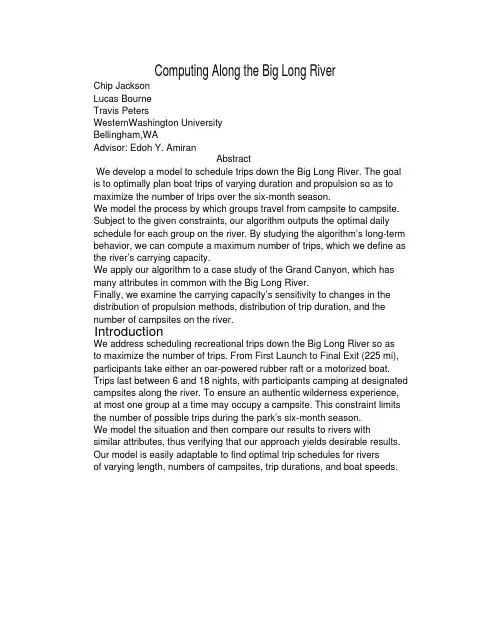
We develop a model to schedule trips down the Big Long River. The goalComputing Along the Big Long RiverChip JacksonLucas BourneTravis PetersWesternWashington UniversityBellingham,WAAdvisor: Edoh Y. AmiranAbstractis to optimally plan boat trips of varying duration and propulsion so as tomaximize the number of trips over the six-month season.We model the process by which groups travel from campsite to campsite.Subject to the given constraints, our algorithm outputs the optimal dailyschedule for each group on the river. By studying the algorithm’s long-termbehavior, we can compute a maximum number of trips, which we define asthe river’s carrying capacity.We apply our algorithm to a case study of the Grand Canyon, which hasmany attributes in common with the Big Long River.Finally, we examine the carrying capacity’s sensitivity to changes in thedistribution of propulsion methods, distribution of trip duration, and thenumber of campsites on the river.IntroductionWe address scheduling recreational trips down the Big Long River so asto maximize the number of trips. From First Launch to Final Exit (225 mi),participants take either an oar-powered rubber raft or a motorized boat.Trips last between 6 and 18 nights, with participants camping at designatedcampsites along the river. To ensure an authentic wilderness experience,at most one group at a time may occupy a campsite. This constraint limitsthe number of possible trips during the park’s six-month season.We model the situation and then compare our results to rivers withsimilar attributes, thus verifying that our approach yields desirable results.Our model is easily adaptable to find optimal trip schedules for riversof varying length, numbers of campsites, trip durations, and boat speeds.No two groups can occupy the same campsite at the same time.Campsites are distributed uniformly along the river.Trips are scheduled during a six-month period of the year.Group trips range from 6 to 18 nights.Motorized boats travel 8 mph on average.Oar-powered rubber rafts travel 4 mph on average.There are only two types of boats: oar-powered rubber rafts and motorizedTrips begin at First Launch and end at Final Exit, 225 miles downstream.*simulates river-trip scheduling as a function of a distribution of trip*can be applied to real-world rivers with similar attributes (i.e., the Grand*is flexible enough to simulate a wide range of feasible inputs; andWhat is the carrying capacity of the riverÿhe maximum number ofHow many new groups can start a river trip on any given day?How should trips of varying length and propulsion be scheduled toDefining the Problemmaximize the number of trips possible over a six-month season?groups that can be sent down the river during its six-month season?Model OverviewWe design a model thatCanyon);lengths (either 6, 12, or 18 days), a varying distribution of propulsionspeeds, and a varying number of campsites.The model predicts the number of trips over a six-month season. It alsoanswers questions about the carrying capacity of the river, advantageousdistributions of propulsion speeds and trip lengths, how many groups canstart a river trip each day, and how to schedule trips.ConstraintsThe problem specifies the following constraints:boats.AssumptionsWe can prescribe the ratio of oar-powered river rafts to motorized boats that go onto the river each day.There can be problems if too many oar-powered boats are launched with short trip lengths.The duration of a trip is either 12 days or 18 days for oar-powered rafts, and either 6 days or 12 days for motorized boats.This simplification still allows our model to produce meaningful results while letting us compare the effect of varying trip lengths.There can only be one group per campsite per night.This agrees with the desires of the river manager.Each day, a group can only move downstream or remain in its current campsiteÿt cannot move back upstream.This restricts the flow of groups to a single direction, greatly simplifying how we can move groups from campsite to campsite.Groups can travel only between 8 a.m. and 6 p.m., a maximum of 9hours of travel per day (one hour is subtracted for breaks/lunch/etc.).This implies that per day, oar-powered rafts can travel at most 36 miles, and motorized boats at most 72 miles. This assumption allows us to determine which groups can reasonably reach a given campsite.Groups never travel farther than the distance that they can feasibly travelin a single day: 36 miles per day for oar-powered rafts and 72 miles per day for motorized boats.We ignore variables that could influence maximum daily travel distance, such as weather and river conditions.There is no way of accurately including these in the model.Campsites are distributed uniformly so that the distance between campsites is the length of the river divided by the number of campsites.We can thus represent the river as an array of equally-spaced campsites.A group must reach the end of the river on the final day of its trip:A group will not leave the river early even if able to.A group will not have a finish date past the desired trip length.This assumption fits what we believe is an important standard for theriver manager and for the quality of the trips.MethodsWe define some terms and phrases:Open campsite: Acampsite is open if there is no groupcurrently occupying it: Campsite cn is open if no group gi is assigned to cn.Moving to an open campsite: For a group gi, its campsite cn, moving to some other open campsite cm ÿ= cn is equivalent to assigning gi to the new campsite. Since a group can move only downstream, or remain at their current campsite, we must have m ÿ n.Waitlist: The waitlist for a given day is composed of the groups that are not yet on the river but will start their trip on the day when their ranking onthe waitlist and their ability to reach a campsite c includes them in theset Gc of groups that can reach campsite c, and the groups are deemed “the highest priority.” Waitlisted groups are initialized with a current campsite value of c0 (the zeroth campsite), and are assumed to have priority P = 1 until they are moved from the waitlist onto the river.Off the River: We consider the first space off of the river to be the “final campsite” cfinal, and it is always an open campsite (so that any number of groups can be assigned to it. This is consistent with the understanding that any number of groups can move off of the river in a single day.The Farthest Empty CampsiteOurscheduling algorithm uses an array as the data structure to represent the river, with each element of the array being a campsite. The algorithm begins each day by finding the open campsite c that is farthest down the river, then generates a set Gc of all groups that could potentially reach c that night. Thus,Gc = {gi | li +mi . c},where li is the groupÿs current location and mi is the maximum distance that the group can travel in one day.. The requirement that mi + li . c specifies that group gi must be able to reach campsite c in one day.. Gc can consist of groups on the river and groups on the waitlist.. If Gc = ., then we move to the next farthest empty campsite.located upstream, closer to the start of the river. The algorithm always runs from the end of the river up towards the start of the river.. IfGc ÿ= ., then the algorithm attempts tomovethe groupwith the highest priority to campsite c.The scheduling algorithm continues in this fashion until the farthestempty campsite is the zeroth campsite c0. At this point, every group that was able to move on the river that day has been moved to a campsite, and we start the algorithm again to simulate the next day.PriorityOnce a set Gc has been formed for a specific campsite c, the algorithm must decide which group to move to that campsite. The priority Pi is a measure of how far ahead or behind schedule group gi is:. Pi > 1: group gi is behind schedule;. Pi < 1: group gi is ahead of schedule;. Pi = 1: group gi is precisely on schedule.We attempt to move the group with the highest priority into c.Some examples of situations that arise, and how priority is used to resolve them, are outlined in Figures 1 and 2.Priorities and Other ConsiderationsOur algorithm always tries to move the group that is the most behind schedule, to try to ensure that each group is camped on the river for aFigure 1. The scheduling algorithm has found that the farthest open campsite is Campsite 6 and Groups A, B, and C can feasibly reach it. Group B has the highest priority, so we move Group B to Campsite 6.Figure 2. As the scheduling algorithm progresses past Campsite 6, it finds that the next farthest open campsite is Campsite 5. The algorithm has calculated that Groups A and C can feasibly reach it; since PA > PC, Group A is moved to Campsite 5.number of nights equal to its predetermined trip length. However, in someinstances it may not be ideal to move the group with highest priority tothe farthest feasible open campsite. Such is the case if the group with thehighest priority is ahead of schedule (P <1).We provide the following rules for handling group priorities:?If gi is behind schedule, i.e. Pi > 1, then move gi to c, its farthest reachableopen campsite.?If gi is ahead of schedule, i.e. Pi < 1, then calculate diai, the number ofnights that the group has already been on the river times the averagedistance per day that the group should travel to be on schedule. If theresult is greater than or equal (in miles) to the location of campsite c, thenmove gi to c. Doing so amounts to moving gi only in such a way that itis no longer ahead of schedule.?Regardless of Pi, if the chosen c = cfinal, then do not move gi unless ti =di. This feature ensures that giÿ trip will not end before its designatedend date.Theonecasewhere a groupÿ priority is disregardedisshownin Figure 3.Scheduling SimulationWe now demonstrate how our model could be used to schedule rivertrips.In the following example, we assume 50 campsites along the 225-mileriver, and we introduce 4 groups to the river each day. We project the tripFigure 3. The farthest open campsite is the campsite off the river. The algorithm finds that GroupD could move there, but GroupD has tD > dD.that is, GroupD is supposed to be on the river for12 nights but so far has spent only 11.so Group D remains on the river, at some campsite between 171 and 224 inclusive.schedules of the four specific groups that we introduce to the river on day25. We choose a midseason day to demonstrate our modelÿs stability overtime. The characteristics of the four groups are:. g1: motorized, t1 = 6;. g2: oar-powered, t2 = 18;. g3: motorized, t3 = 12;. g4: oar-powered, t4 = 12.Figure 5 shows each groupÿs campsite number and priority value foreach night spent on the river. For instance, the column labeled g2 givescampsite numbers for each of the nights of g2ÿs trip. We find that each giis off the river after spending exactly ti nights camping, and that P ÿ 1as di ÿ ti, showing that as time passes our algorithm attempts to get (andkeep) groups on schedule. Figures 6 and 7 display our results graphically.These findings are consistent with the intention of our method; we see inthis small-scale simulation that our algorithm produces desirable results.Case StudyThe Grand CanyonThe Grand Canyon is an ideal case study for our model, since it sharesmany characteristics with the Big Long River. The Canyonÿs primary riverrafting stretch is 226 miles, it has 235 campsites, and it is open approximatelysix months of the year. It allows tourists to travel by motorized boat or byoar-powered river raft for a maximum of 12 or 18 days, respectively [Jalbertet al. 2006].Using the parameters of the Grand Canyon, we test our model by runninga number of simulations. We alter the number of groups placed on thewater each day, attempting to find the carrying capacity for the river.theFigure 7. Priority values of groups over the course of each trip. Values converge to P = 1 due to the algorithm’s attempt to keep groups on schedule.maximumnumber of possible trips over a six-month season. The main constraintis that each trip must last the group’s planned trip duration. Duringits summer season, the Grand Canyon typically places six new groups onthe water each day [Jalbert et al. 2006], so we use this value for our first simulation.In each simulation, we use an equal number of motorized boatsand oar-powered rafts, along with an equal distribution of trip lengths.Our model predicts the number of groups that make it off the river(completed trips), how many trips arrive past their desired end date (latetrips), and the number of groups that did not make it off the waitlist (totalleft on waitlist). These values change as we vary the number of new groupsplaced on the water each day (groups/day).Table 1 indicates that a maximum of 18 groups can be sent down theriver each day. Over the course of the six-month season, this amounts to nearly 3,000 trips. Increasing groups/day above 18 is likely to cause latetrips (some groups are still on the river when our simulation ends) and long waitlists. In Simulation 1, we send 1,080 groups down river (6 groups/day?80 days) but only 996 groups make it off; the other groups began near the end of the six-month period and did not reach the end of their trip beforethe end of the season. These groups have negligible impact on our results and we ignore them.Sensitivity Analysis of Carrying CapacityManagers of the Big Long River are faced with a similar task to that of the managers of the Grand Canyon. Therefore, by finding an optimal solutionfor the Grand Canyon, we may also have found an optimal solution forthe Big Long River. However, this optimal solution is based on two key assumptions:?Each day, we put approximately the same number of groups onto theriver; and?the river has about one campsite per mile.We can make these assumptions for the Grand Canyon because they are true for the Grand Canyon, but we do not know if they are true for the Big Long River.To deal with these unknowns,wecreate Table 3. Its values are generatedby fixing the number Y of campsites on the river and the ratio R of oarpowered rafts to motorized boats launched each day, and then increasingthe number of trips added to the river each day until the river reaches peak carrying capacity.The peak carrying capacities in Table 3 can be visualized as points ina three-dimensional space, and we can find a best-fit surface that passes (nearly) through the data points. This best-fit surface allows us to estimatethe peak carrying capacity M of the river for interpolated values. Essentially, it givesM as a function of Y and R and shows how sensitiveM is tochanges in Y and/or R. Figure 7 is a contour diagram of this surface.The ridge along the vertical line R = 1 : 1 predicts that for any givenvalue of Y between 100 and 300, the river will have an optimal value ofM when R = 1 : 1. Unfortunately, the formula for this best-fit surface is rather complex, and it doesn’t do an accurate job of extrapolating beyond the data of Table 3; so it is not a particularly useful tool for the peak carrying capacity for other values ofR. The best method to predict the peak carrying capacity is just to use our scheduling algorithm.Sensitivity Analysis of Carrying Capacity re R and DWe have treatedM as a function ofR and Y , but it is still unknown to us how M is affected by the mix of trip durations of groups on the river (D).For example, if we scheduled trips of either 6 or 12 days, how would this affect M? The river managers want to know what mix of trips of varying duration and speed will utilize the river in the best way possible.We use our scheduling algorithm to attempt to answer this question.We fix the number of campsites at 200 and determine the peak carrying capacity for values of R andD. The results of this simulation are displayed in Table 4.Table 4 is intended to address the question of what mix of trip durations and speeds will yield a maximum carrying capacity. For example: If the river managers are currently scheduling trips of length?6, 12, or 18: Capacity could be increased either by increasing R to be closer to 1:1 or by decreasing D to be closer to ? or 12.?12 or 18: Decrease D to be closer to ? or 12.?6 or 12: Increase R to be closer to 4:1.ConclusionThe river managers have asked how many more trips can be added tothe Big Long Riverÿ season. Without knowing the specifics ofhowthe river is currently being managed, we cannot give an exact answer. However, by applying our modelto a study of the GrandCanyon,wefound results which could be extrapolated to the context of the Big Long River. Specifically, the managers of the Big Long River could add approximately (3,000 - X) groups to the rafting season, where X is the current number of trips and 3,000 is the capacity predicted by our scheduling algorithm. Additionally, we modeled how certain variables are related to each other; M, D, R, and Y . River managers could refer to our figures and tables to see how they could change their current values of D, R, and Y to achieve a greater carrying capacity for the Big Long River.We also addressed scheduling campsite placement for groups moving down the Big Long River through an algorithm which uses priority values to move groups downstream in an orderly manner.Limitations and Error AnalysisCarrying Capacity OverestimationOur model has several limitations. It assumes that the capacity of theriver is constrained only by the number of campsites, the trip durations,and the transportation methods. We maximize the river’s carrying capacity, even if this means that nearly every campsite is occupied each night.This may not be ideal, potentially leading to congestion or environmental degradation of the river. Because of this, our model may overestimate the maximum number of trips possible over long periods of time. Environmental ConcernsOur case study of the Grand Canyon is evidence that our model omits variables. We are confident that the Grand Canyon could provide enough campsites for 3,000 trips over a six-month period, as predicted by our algorithm. However, since the actual figure is around 1,000 trips [Jalbert et al.2006], the error is likely due to factors outside of campsite capacity, perhaps environmental concerns.Neglect of River SpeedAnother variable that our model ignores is the speed of the river. Riverspeed increases with the depth and slope of the river channel, makingour assumption of constant maximum daily travel distance impossible [Wikipedia 2012]. When a river experiences high flow, river speeds can double, and entire campsites can end up under water [National Park Service 2008]. Again, the results of our model don’t reflect these issues. ReferencesC.U. Boulder Dept. of Applied Mathematics. n.d. Fitting a surface to scatteredx-y-z data points. /computing/Mathematica/Fit/ .Jalbert, Linda, Lenore Grover-Bullington, and Lori Crystal, et al. 2006. Colorado River management plan. 2006./grca/parkmgmt/upload/CRMPIF_s.pdf .National Park Service. 2008. Grand Canyon National Park. High flowriver permit information. /grca/naturescience/high_flow2008-permit.htm .Sullivan, Steve. 2011. Grand Canyon River Statistics Calendar Year 2010./grca/planyourvisit/upload/Calendar_Year_2010_River_Statistics.pdf .Wikipedia. 2012. River. /wiki/River .Memo to Managers of the Big Long RiverIn response to your questions regarding trip scheduling and river capacity,we are writing to inform you of our findings.Our primary accomplishment is the development of a scheduling algorithm.If implemented at Big Long River, it could advise park rangerson how to optimally schedule trips of varying length and propulsion. Theoptimal schedule will maximize the number of trips possible over the sixmonth season.Our algorithm is flexible, taking a variety of different inputs. Theseinclude the number and availability of campsites, and parameters associatedwith each tour group. Given the necessary inputs, we can output adaily schedule. In essence, our algorithm does this by using the state of theriver from the previous day. Schedules consist of campsite assignments foreach group on the river, as well those waiting to begin their trip. Given knowledge of future waitlists, our algorithm can output schedules monthsin advance, allowing managementto schedule the precise campsite locationof any group on any future date.Sparing you the mathematical details, allow us to say simply that ouralgorithm uses a priority system. It prioritizes groups who are behindschedule by allowing them to move to further campsites, and holds backgroups who are ahead of schedule. In this way, it ensures that all trips willbe completed in precisely the length of time the passenger had planned for.But scheduling is only part of what our algorithm can do. It can alsocompute a maximum number of possible trips over the six-month season.We call this the carrying capacity of the river. If we find we are below ourcarrying capacity, our algorithm can tell us how many more groups wecould be adding to the water each day. Conversely, if we are experiencingriver congestion, we can determine how many fewer groups we should beadding each day to get things running smoothly again.An interesting finding of our algorithm is how the ratio of oar-poweredriver rafts to motorized boats affects the number of trips we can send downstream. When dealing with an even distribution of trip durations (from 6 to18 days), we recommend a 1:1 ratio to maximize the river’s carrying capacity.If the distribution is skewed towards shorter trip durations, then ourmodel predicts that increasing towards a 4:1 ratio will cause the carryingcapacity to increase. If the distribution is skewed the opposite way, towards longer trip durations, then the carrying capacity of the river will always beless than in the previous two cases—so this is not recommended.Our algorithm has been thoroughly tested, and we believe that it isa powerful tool for determining the river’s carrying capacity, optimizing daily schedules, and ensuring that people will be able to complete their trip as planned while enjoying a true wilderness experience.Sincerely yours,Team 13955。
2012 MCM ProblemsPROBLEM A:The Leaves of a Tree"How much do the leaves on a tree weigh?" How might one estimate the actual weight of the leaves (or for that matter any other parts of the tree)? How might one classify leaves? Build a mathematical mode l to describe and classify leaves. Consider and answer the following:• Why do leaves have the various shapes that they have?• Do the shapes “minimize” overlapping individual shadows that are cast, so as to maximize exposure? Does the distribution of leaves within the “volume” of the tree and its branches effect the shape?• Speaking of profiles, is leaf shape (general characteristics) related to tree profile/branching structure?• How would you estimate the leaf mass of a tree? Is there a correlation between the leaf mass and the size characteristics of the tree (height, mass, volume defined by the profile)?In addition to your one page summary sheet prepare a one page letter to an editor of a scientific journal outlining your key findings.“多少钱树的叶子有多重?”怎么可能估计的叶子(或树为此事的任何其他部分)的实际重量?会如何分类的叶子吗?建立了一个数学模型来描述和分类的叶子。

2012年美国数学建模题目中文版第一篇:2012年美国数学建模题目解析2012年美国数学建模竞赛题目分为3个部分:A、B、C 部分,其中A、B两部分每个题目都设计成了开放式问题,而C部分则是两道严谨的数学证明题目。
A部分共有四个问题,分别为:1、搜索引擎的自动补充功能对于使用者的输入进行了什么样的预测和补全?如果这种功能可以被改变,在搜索引擎中进行必要的优化,会对搜索引擎的使用产生什么影响?2、在一个公共交通的网络中,如何合理地分配车辆保证所有的车辆在一定时间内都能够按时到达各自的终点站?3、如何在餐馆排队时,给不同的桌子和不同的人分配最佳位置,以便让顾客在餐厅等待的时间最短?4、针对特定的树木,如何编写算法来找到该树生长的变化,在叶片的数量和大小、气孔的数量和大小等方面的特征?对于这四个问题,考生需要通过分析问题,理清思路,构思模型,进行数据分析,最后得出自己的结论。
需要注意的是,每个问题都是非常开放式的,没有标准答案,最终得分并不会仅仅取决于观点是否正确,具体的解题过程、数据展示和准确度也是非常关键的。
B部分共有三个问题,分别为:1、如何通过旅游者在社交网络上的信息,帮助旅游者更好地定制旅游计划?2、如何在残缺不全的传媒报道中,找到事实并从中解读该事件?3、针对滑雪者在滑雪过程中的各种情况,如何预测他们的滑雪技巧以及未来的滑雪表现?对于B部分的三个问题,其实也都是很自由的问题,可以根据自己所擅长领域进行分析,构思自己的模型和算法,注重细节和数据展示。
C部分共有两个题目:1、已知一个最小二乘问题,其正则化后的解为稀疏的,试设计一个迭代算法在有效的处理机制下对其进行数值求解。
2、已知一个对象向一条线段上匀速运动,在线段的中途,运动的对象突然重力下落,如果目标是在最短的时间内捕捉该运动的对象,该怎样运动才是最优策略?对于C部分两个题目,需要在数学基础扎实的基础上进行思考,深入分析,构建出严谨的证明过程,注重逻辑和方法。
SummaryMany scholars conclude that leaf shape is highly related with the veins. Based on this theory, we assume the leaf growth in each direction satisfies a function. For the leaves in the same tree, the parameters are different; for those of separate trees, the function mode is different. Thus the shape of leaf differs from that of another. In the end of section 3, we simulate one growing period and depict the leaf shape.Through thousands of years of evolution, the leaves find various wa ys to make a full use of natural resources, including minimizing overlapping individual shadows. In order to find the main factors promoting the evolution of leaves, we analyze the distribution of adjacent leaves and the equilibrium point of photosynthesis and respiration. Besides, we also make a coronary hierarchical model and transmission model of the solar radiation to analyze the influence of the branches.As to the tree structure and the leaf shape, first we consider one species. Different tree shapes have different space which is built up by the branch quality and angle, effect light distribution, ventilation and humidity and concentration of CO2 in the tree crown. These are the factors which affect the leaf shape according to the model in section 1. Here we analyze three typical tree shapes: Small canopy shape, Open center shape and Freedom spindle shape, which can be described by BP network and fractional dimension model. We find that the factors mainly affect the function of Sthat affects the additional leaf area. Factors are assembled in different ways to create different leaf shapes. So that the relationship between leaf shape and tree profile/branching structure is proved.Finally we develop a model to calculate the leaf mass from the basic formula of . By adjusting the crown of a tree to a half ellipsoid, we first define thefunction of related factors,such as the leaf density and the effective ratio of leaf area. Then we develop the model using calculus. With this model, weapproximately evaluate the leaf mass of a middle-sized tree is 141kg.Dear editor,How much the leaves on a tree weigh is the focus of discussion all the time. Our team study on the theme following the current trend and we find something interesting in the process.The tree itself is component by many major elements. In our findings, we analyze the leaf mass with complicated ones, like leaf shape, tree structure and branch characteristics, which interlace with each other.With the theory that leaf shape is highly related with the veins, we assume theleaf growth in each direction satisfies a function . For the leaves in thesame tree, the parameters are different; for those of separate trees, the function mode is di fferent. That’s why no leaf shares the same shape. Also, we simulate one growing period and depict the leaf shape.In order to find the main factors promoting the evolution of leaves, we analyze the distribution of adjacent leaves and the equilibrium point of photosynthesis and respiration. Besides, we also make a coronary hierarchical model and transmission model of the solar radiation to analyze the influence of the branches.As to the tree structure and the leaf shape, different tree shapes have differe nt space which is built up by the branch quality and angle, effect light distribution, ventilation and humidity and concentration of CO2 in the tree crown that affect leaf shapes. Here we analyze three typical tree shapes which can be described by BP network and fractional dimension model. We find that the factors mainly affect the function of Sthat affects the additional leaf area. Factors are assembled in different ways to create different leaf shapes. So that the relationship between leaf shape and tree profile or branching structure is proved.Finally we develop the significant model to calculate the leaf mass from thebasic formula of . By adjusting the crown of a tree to a half ellipsoid,we first define the function of related factors and then we develop the model using calculus. With this model, we approximately evaluate the leaf mass of a middle-sized tree is 141kg.We are greatly appreciated that if you can take our findings into consideration. Thank you very much for your precious time for reading our letter.Yours sincerely,Team #14749Contents1. Introduction (4)2. Parameters (4)3. Leaves have their own shapes (5)3.1 Photosynthesis is important to plants (5)3.2 How leaves grow? (6)3.3 Build our model (7)3.4 A simulation of the model (10)4. Do the shapes maximize exposure? (14)4.1 The optimum solution of reducing overlapping shadows (14)4.1.1 The distribution of adjacent leaves (14)4.1.2 Equilibrium point of photosynthesis and respiration (15)4.2 The influence of the “volume” of a tree and its branches (17)4.2.1 The coronary hierarchical model (17)4.2.2 Spatial distribution model of canopy leaf area (18)4.2.3 Transmission model of the solar radiation (19)5. Is leaf shape related to tree structure? (20)5.1 The experiment for one species (21)5.2 Different tree shapes affect the leaf shapes (23)5.2.1 The light distribution in different shapes (23)5.2.2 Wind speed and humidity in the canopy (23)5.2.3 The concentration of carbon dioxide (24)5.3 Conclusion and promotion (25)6. Calculus model for leaf mass (26)6.1 How to estimate the leaf mass? (26)6.2 A simulation of the model (28)7. Strengths and Weakness (29)7.1 Strengths (29)7.2 Weaknesses (30)8. Reference (30)1. IntroductionHow much do the leaves on a tree weigh? Why do leaves have the various shapes that they have? How might one estimate the actual weight of the leaves? How might one classify leaves?We human-beings have never stopped our steps on exploring the natural world. But, as a matter of fact, the answer to those questions is still unresolved. Many scientists continue to study on this area. Recently , Dr. Benjamin Blonder (2010) achieved a new breakthrough on the venation networks and the origin of the leaf econo mics spectrum. They defined a standardized set of traits – density , distance and loopiness and developed a novel quantitative model that uses these venation traits to model leaf-level physiology .Now, it is commonly thought that there are four key leaf functional traits related to leaf economics: net carbon assimilation rate, life span, leaf mass per area ratio and nitrogen content.2. Parametersthe area a leaf grows decided by photosynthesisthe additional leaf area in one growing periodthe leaf growing obliquity Pthe total photosynthetic rate 0d R the dark respiration rate of leavesn P the net photosynthetic rateh the height of the canopyd the distance between two branchesdi the illumination intensity of scattered light from a given directionthe solar zenith angleh the truck highh the crown high13. Leaves have their own shapes3.1 Photosynthesis is important to plantsIt is widely accepted that two leaves are different, no matter where they are chosen from; even they are from the very tree. To understand how leaves grow is helpful to answer why leaves have the various shapes that they have.The canopy photosynthesis and respiration are the central parts of most biophysical crop and pasture simulation models. In most models, the acclamatory responses of protein and the environmental conditions, such as light, temperature and CO2 concentration, are concerned[1].In 1980, Farquhar et al developed a model named FvCB model to describe photosynthesis[2]:The FvCB model predicts the net assimilation rate by choosing the minimum between the Rubisco-limited net photosynthetic rate and the electron transport-limited net photosynthetic rate.Assume A n, A c, A j are the symbols for net assimilation rate, the Rubisco-limited net photosynthetic rate and the electron transport-limited net photosynthetic rate respectively, and the function can be described as:(1)(2)where and are the intercellular partial pressures of CO2 and O2,respectively, and are the Michaelis–Menten coefficients ofRubisco for CO2and O2, respectively, is the CO2compensation point inthe absence of (day respiration in andis the photosystem II electron transport rate that is used for CO2fixation and photorespiration[3][4].We apply the results of this model to build the relationship between the photosynthesis and the area a leaf grows during a period of time. It can be released as:(3)and are the area of the target leaf and the period of time it grows.is a function which can transfer the amount ofCO2into the area the leaf grows and the are parameters which affect S p. S p can be used as a constraint condition in our model.3.2 How leaves grow?As the collocation of computer hardware and software develops, people can refer to bridging biology, morphogenesis, applied mathematics and computer graphics to simulate living organisms[5], thus how to model leaves is of great challenge. In 2001, Dengler and Kang[6]brought up the thought that leaf shape is highly related to venation patterns. Recently, Runions[7] brought up a method to portray the leaf shape by analyzing venation patterns. Together with the Lindenmayer system (L-system), an advanced venation model can adjust the growth better that it solved the problem occurred in the previous model that the secondary veins are retarded.We knowleaves have various shapes.For example, leaves can be classified in to simple leaves which have an undivided blade and compound leaves whose blade is divided into two or more distinctleaflets such as the Fabaceae. As to the shape of a leaf, it may have marginal dentations of the leaf blades or not, and like a palm with various fingers or an elliptical cake. Judd et al defined a set of terms which describe the shape of leaves as follows [8]:We chose entire leaves to produce this model as a simplification. What’s more, they confirmed again that the growth of venations relates with that of the leaf.To disclose this relationship, Relative Elementary Rate of Growth (RERG) can be introduced to depict leaves growth [9]. RERG is defined as the growth rate per distance, in the definitive direction l at a point p of the growing object, yielding(4)Considered RERG , the growth patterns of leaves are also different. Roth-Nebelsick et al brought up four styles in their paper [10]:3.3 Build our modelWe chose marginal growth to build our model. Amid all above-mentioned studies, weFigure 3.1 Terms pertinent to the description of leaf shapes.Figure 3.2 A sample leaf (a) and the results of its: (b) marginal growth, (c) uniform isotropic (isogonic) growth, (d) uniform anisotropic growth, and (e) non-uniform anisotropic growth.Figure 3.3 The half of a leaf is settled in x-y plane like this with primary vein overlapping x-axis. The leaf grows in the direction of .assume that the leaf produce materials it needs to grow by photosynthesis to expand its leaf area from its border and this process is only affected by what we have discussed in the previous section about photosynthesis. The border can be infinitesimally divided into points. Set as the angle between the x-axis and thestraight line connecting the grid origin and one point on the curve,andas the growth distance in the direction of . To simplify the model, we assume that the leaf grows symmetrical. We put half of the leaf into the x-y plane and make the primary vein overlap x-axis.This is how we assume the leaf grows.In one circle of leaf growth, anything that photosynthesis provided transfers into theadditional leaf area, which can be described as:(5)while in the figure.In this case, we can simulate leaf growth thus define the leaf shape by using iterative operations the times N a leaf grow in its entire circle ①.① For instance, if the vegetative circle of a leaf is 20 weeks on average, the times of iterative operations N can beset as 20 when we calculate on a weekly basis.Figure 3.4 The curves of the adjacent growing period and their relationship.First, we pre-establish the border shape of a leaf in the x-y plane, yielding . where , the relevant satisfies:(6)(7) In the first growing period, assume , the growth distance in the direction of ,satisfies:(8)(9) It releases the relationship of the coordinates in the adjacent growing period. In this case, we can use eq.(9)to predict the new border of the leaf after one period of growth②:(10)And the average simple recursions are③:②That means, in the end of period 1.③As we both change the x coordinate and the y coordinate, in the new period, these two figures relate through those in the last period in the functions.(11)After simulate the leaf borders of the interactive periods, use definite integral ④ to settle parametersin the eq.(8) then can be calculated in each direction of , thus the exact shape of a leaf in the next period is visible.When the number of times N the leaf grows in its life circle applies above-mentioned recursions to iterate N times and the final leaf shape can be settled.By this model, we can draw conclusions about why leaves have different shapes. For the leaves on the same tree, they share the same method of expansion which can be described as the same type of function as Eq.(8). The reason why they are different, not only in a sense of big or small, is that in each growing period they acquire different amount of materials used to expand its own area. In a word, the parameters in the fixedly formed eq.(8) are different for any individual leaf on the same tree. For the leaves of different tree species, the corresponding forms of eq.(8) are dissimilar. Some are linear, some are logarithmic, some are exponential or mixtures of that, which settle the totally different expansion way of leaf, are related with the veins. On that condition, the characters can be divided by a more general concept such as entire or toothed.3.4 A simulation of the modelWe set the related parameters by ourselves to simulate the shape of a leaf and to express the model better.First we initialize the leaf shape by simulating the function of a leaf border at the④The relationship must meet eq.(5).Figure 3.5 and the recurrence relations.beginning of growing period 1 in the x-y plane. By observation, we assume that themovement of the initial leaf border satisfied:(12)Suppose the curve goes across the origin of coordinates, then the constraint conditionscan be:(13)Thus the solution to eq.(13) is:(14)By using Mathematica we calculatewhereandthe area of the half leaf is: (15)Wesettleaccording to the research by S. V . Archontoulisin et al [11] in eq.(3). On a weekly basis, theparameter. In eq.(15), we have .Figure 3.6When assume ,thus constraint condition eq.(5) becomes: (16)When eq.(8) is linear and after referring to Runions’s paper, we assume that Y -valuedecreases when X-value increases, which means the leaf grows faster at the end of theprimary vein. If the grow rate at the end of the primary vein is 0,as ,eq.(8) can be described as: (17)where b is decided by eq.(16).To settle the value of b , we calculate multiple sets of data by Excel then use a planecurve to trace them and get the approximation of b . In this method, we use grid toapproximate .Apparently,is monotone.When b is 2: The square of each square is 0.0139cm 2, and the total number of the squares in theadditional area is about 240. SoFigure 3.7When b is 2.5:Thesquare of each squareis 0.0240cm 2, and the total number of the squares in theadditional area is about 201. SoWhen b is 3:The square of each square is 0.0320cm 2, and the total number of the squares in the additional area is about 193. SoAfter comparing, we can draw a conclusion that fit eq.(16)best; accordingly, in period 1: (18)In each growing period, may be different for the amount of material produced isFigure 3.9Figure 3.8related with various factors, such as the change of relative location and CO 2 or O 2concentration, and other reasons. By using the same method, the leaf shape in period2 or other period can be generated on the basis of the previous growing period untilthe end of its life circle.What’s more, when eq.(8) is remodeled, the corresponding leaf shape can be changed.With , the following figure shows the transformationof a leaf shape in the firstgrowing period with the samesettled above and we can see that the shape will be dissected in the end.4. Do the shapes maximize exposure?4.1 The optimum solution of reducing overlapping shadows4.1.1 The distribution of adjacent leavesV ein is the foundation of the leaves. With the growing of veins, the leaves graduallyexpand around. The distribution of main and lateral veins plays an important decisiverole in the shapes of leaves. The scientists created a mathematical model which usesthree decisive factors - the relationship between the rate of photosynthesis, leaf life,carbon consumption or nitrogen consumption, to simulate the leaves’ shape. Becauseof carbon consumption is a constant for one tree, and we take the neighboring leavesin the same growth cycle to observe. So, we can only focus on one factor - the rate ofphotosynthesis.Figure 3.10The shape differs from figure 3.7-3.9, as the kind offunction of is different. In this case, it is a cubic model while a linear model in figure 3.7-3.9.Through the observation of dicotyledon, leaves on a branch will grow in a staggered way that can reduce the overlapping individual shadows of adjacent leaves and make them get more sunlight (Figure 4.1).Figure 4.1 The rotation distribution of leavesBase on the similar environment, we assume that adjacent leaves nearly have the same shape. From the perspective of looking down, the leaves grow from a point on the branch. So, we can simplify the vertical view of leaves as a circle of which the radius is the length of a vein which is represented with r. The width of the leaf is represented with w. The angle between two leaves is represented with β(Figure4.2).Figure 4.2 The vertical view of leavesThe leaves should use the space as much as possible, and for the leaf with one main vein, oval is the best choice. In general, βis between 15°and 90°. In this way, effectively reduce the direct overlapping area. According to the analysis of the first question, r and w are determined by the rate of photosynthesis and respiration. Besides, the width of leaf is becoming narrower when the main vein turns to be thinner.4.1.2 Equilibrium point of photosynthesis and respirationThe organism produced by photosynthesis firstly satisfies needs of leaf itself. Then the remaining organism delivered to the root to meet the growth needs of the tree. As we know, respiration needs to consume organism. If the light is not sufficient, organism produced by photosynthesis may no longer be able to afford the materials required for the growth of leaves. There should be an equilibrium point so as toprevent the leaf is behindhand in its circumstances.The formula [12] that describes the photosynthetic rate in response to light intensity with gradual exponential growth index can be expressed as:(19) Where P is total photosynthetic rate, m ax P is maximum photosynthetic rate ofleaves, a is initial solar energy utilization and I is photosynthetic photon quanta flux density .The respiration rate is affected by temperature ,using the formal of index to describe as follows:025102T d d R R -=⋅ (20)Where T is temperature and 0d R is the dark respiration rate of leaves, when the temperature is 25 degrees. As a model parameter, 0d R can be determined bynonlinear fitting. Therefore, the net photosynthetic rate can be expressed in the indexform as follows:(21)Where n P is the net photosynthetic rate, which does not include the concentration ofcarbon dioxide and other factors. The unit of n P is 21m ol m s μ--⋅⋅.We assume that the space for leaf growth is limited, the initial area of the leaf is 0S . At this point, the entire leaf happens to be capable of receiving sunlight. If the leaf continue to grow, some part of the leaf will be in the shadows and the area in the shadows is represented with x . Ignore the fluctuation cycle of photosynthesis and respiration, on average, the duration of photosynthesis is six hours per day . In the meanwhile, the respiration is ongoing all the time. When the area increased to S , we established an equation as follows:(22)where μ is the remaining organism created by the leaf per day . And from where 0μ=, which means the organism produced by photosynthesis has all been broken down completely in the respiration, we get the equilibrium point.4n n d S P x P R ⋅=+ (23) The proportion of the shaded area in the total area:4nn d P xS P R =+ (24)Cite an example of oak trees, we found the following data (Figure 4.3), which shows the relationship between net photosynthesis and dark respiration during 160 days. Thehabitat of the trees is affected by the semi-humid monsoon climate.Figure 4.3 The diurnal rate of net photosynthesis and dark respiration [13]In general, 217n P m ol m s μ--=⋅⋅,214d R m ol m s μ--=⋅⋅. Taking the given numbersinto the equation, we can get the result.0025xS =From the result, we can see that in the natural growth of leaves, with the weakening of photosynthesis, the leaves will naturally stop growing once they come across the blade between blocked. Therefore, the leaves can always keep overlapping individual shadows about 25%, so as to maximize exposure.4.2 The influence of the “volume” of a tree and its branches4.2.1 The coronary hierarchical modelMr. Bōken and Dr. J. Fischer (1987) found that in order to adequate lighting, leaves have different densities and the branches is distributed according to certain rules. They observed tropical plants in Miami, found that the ratio of main branch and two side branches is 1:0.94:0.87, and the angles between them are 24.4°and 36.9°. According to the computer simulation, the two angles can maximize the exposure of leaves.For simply, we use hemisphere to simulate the shape of the canopy. According to the light transmittance rate, we can divide the canopy into outer and inner two layers(Figure 4.3). The volume of the hemisphere depends on the size and distribution of branches.Figure 4.3 The coronary hierarchical modelThe angle between the branches will affect the depth of penetration of sun radiation and the distribution of leaves. Besides, thickness of the branches will affect the transfer of nutrients to the leaves.4.2.2 Spatial distribution model of canopy leaf areaAssume that the distribution of leaves is uniform in the section xz but not uniform in the y direction, as the figure 4.3. Then, we can get the formula of leaf area index (LAI) as follows [14]:/20/21(,)h d d dz x z dx LAI d -∂=⎰⎰(25)Where h is the height of the canopy , d is the distance between two branches, and (,)x z ∂ is the leaf area density function of the micro-body at the point (,)x z . x a is the function of leaf area which means the distribution of cross-section of the X direction, and Its value is a dimensionless, defined as follows: /2/21()d x d a x dx LAI d -=⎰ (26)()()x s a x d LAI C x =⋅⋅ (27)For the canopy which is not uniform in the horizontal direction, the distribution of its leaves is not entirely clear. We use s C to represent the distribution function of thedensity of leaves. s C can be expressed as a quadratic function or a Gaussiandistribution function.4.2.3 Transmission model of the solar radiationAssume that the attenuation of the solar radiation accords with the law of Beer-Lambert. The attenuation value at a point of canopy where the light arrives with a certain angle of incidence and azimuth is proportional to the length of the path, and the length can be calculated by Goudriaan function. Approximate function of the G function is shown as follows [15]:00(12)cos G G k G θ=+- (28)where k is a parameter decided by different plants.Take a micro unit in the canopy . Direct sunlight intercepted in this micro unit can be expressed in the following form:()(,)b b L dI I z G z dLAI =-Θ (29)Where b I means the direct sunlight, Θ is the solar zenith angle and L dL A I is the LAI on the path of light.Figure 4.4 Micro unit of the canopyThrough the integral and the chain rule, we can get the transmittance at the point (',')x z as follows:(,)[()]tan sin ()(',')exp()()h b b z G z a x z a z I x z I h ΘΘ∆Φ+=-⎰ (30)Average direct transmission rate:/2/21(')(',')'d b b d t z t x z dx d --=⎰(31)Different with the direct light, the scattered light in all directions is intercepted by theleaf surface from the upper hemisphere. The irradiance d dI of scattering at the point(',')x z can be expressed as follows:'cos d d b dI i t d ωθ=⋅⋅ (32) where d i is the illumination intensity of scattered light from a given direction.The transmission rate of the sun scattered light is as follows:2/2'00(',')1sin cos ()d b d I x z t d d I h ππθθθϕπ=⎰⎰ (33) Average scattering transmission rate:/2/21(')(',')'d d d d t z t x z dx d --=⎰(34)Global solar radiation reaching the canopy with a given depth z :(')()[(1)(')(')]d b d d I z I h k t z k t z ---=-+ (35)According to eq.(30) and eq.(33), the maximum depth the solar radiation can reach has a major link with h and θ. The shape of leaves have a relationship with photosynthesis. So, the h and θ of branches do have an influence on the leaves. Results showed that the light level and light utilization of high stem and open ce nter shape as well as small and sparse canopy shape were better than others .Double canopy shape ,spindle shape and center shape took second place ,while big canopy shape had the lowest light distribution [16].5. Is leaf shape related to tree structure?Due to internal and external factors, there are many kinds of tree shapes in the nature. For example, the apple's tree shape is semi-ellipsoidal, the willow's is hemispherical, the peach's likes a cup, the pine's likes cone and so on. The shape of their leaves varies. The leaf shape of apple is oval, pine's is needle, and the Indus's is palm. Is leaf shape related to tree shape? Even for the same species, there are many kinds of tree shapes. For instance, Small canopy shape, Open center shape, Freedom spindle shape, high stem and open center shape, Double canopy shape and so on. The sizes of leaves are different. Does the tree profile/branching structure effects the leaf shape?5.1 The experiment for one speciesTo solve this problem, we first consider the relationship of one tree species such as apple, which is semi-ellipsoidal. According to the second question, the hemispherical model is further extended to the semi-ellipsoidal model. Every tree individual shows irregularly because of natural and man-made factors, which reflects on the diversity of the crown in the canopy height direction of the changing relationship between the crown and canopy height. Figure 5.1 shows the relationship.Figure5.1 Schematic diagram of tree crown contourWhere 0h means the truck high, 1h means the crown high, 8710,,,,d d d d ⋅⋅⋅ meanscrown diameter. Tree shape with the scale change can be characterized in fractal dimension. Across the same scales, a fixed fractal dimension indicates the boundary shape's self-similarity; on different scales, the change of fractal dimension means that different processes or limiting factor has superiority. (Wiens, 1989)[17] According to the application of BP network and fractional dimension, we describe the tree shapes.[18]According to Li Guodong and Zhang Junke's work which detected and evaluated in different tree shapes of ‘Fuji’ apple. We choose three kinds of tree shapes to study; they are Small canopy shape, Open center shape and Freedom spindle shape as figure5.2 shows.。

2004年A题题目是研究人的指纹相同导致确认身份时产生错误的可能性和因为DNA相同导致产生错误的可能性。
这道题与生物有关。
2004年,美国提出了“科技展望——生物盾国家纳米技术”,针对微分子进行研究,与人体相关的DNA也就成为焦点。
指纹是区分人的重要参数,它由DNA决定,由于现在自然环境改变,人体的DNA也有可能发生变异,这样引起相同指纹出现也是有可能的。
研究这种变异的可能性有利于刑事案件的侦破,提高政府的防御能力等。
本题目可以采用机理分析法来建模。
可以采用计算机模拟人体染色体中的基因排列进而检验、统计排列结果与指纹形成情况B题题目:现在的快通系统在收费站、娱乐公园和其他的地方,正在越来越频繁的使用,来减少人们排队等候的时间,现在我们考虑为一个娱乐公园所设计的快通系统,在一次测试中,这个公园在几个游客比较多的景点旁都设置的快通系统,这个系统的设计创意是对于那些比较热门的景点,可以到旁边的一个机器,将其门票插入后出来一张纸条,上面写着具体的你可以回来时间段,比如说你把你的门票在1:15插到机子里,系统就会告诉你,你可以在3:30-4:30回来,这个时候队伍就比较短,你可以凭你的纸条加入这个队伍,很快就可以进入景点,为了防止游客同时在几个景点使用这个系统。
系统的机器只允许你一次在一个景点排队等候。
现在你是几个被公园雇佣的互相竞争的一个,你的职责是改善快通系统的运行。
很多游客都在抱怨测试期间系统的异常现象,比如说有一次系统提供的回到景点的时间是4小时以后,但是才过一会儿,在相同景点系统提供的时间只有1小时。
在另外一些时候根据快通系统组织起来的游客的等候队伍,就和普通的队伍一样长一样慢。
现在的问题是要提出并且测试一个模型,这个模型能让快通系统的等候纸条的发放能增加人们在公园的乐趣的目的。
问题的一部分就是首先决定衡量不同模型的标准,在你提交的报告里还要附带一份技术性的总结,以便公园的领导在不同的顾问所提出的模型中选择。
2012 ICM ProblemModeling for Crime BustingYour organization, the Intergalactic Crime Modelers (ICM), is investigating a conspiracy to commit a criminal act. The investigators are highly confident they know several members of the conspiracy, but hope to identify the other members and the leaders before they make arrests. The conspirators andthe possible suspected conspirators all work for the same company in a large office complex. The company has been growing fast and making a name for itself in developing and marketing computer software for banks and credit card companies. ICM has recently found a small set of messages from a group of 82 workers in the company that they believe will help them find the most likely candidates forthe unidentified co‐conspirators and unknown leaders. Since the message traffic is for all the office workers in the company, it is very likely that some (maybe many) of the identified communicators in the message traffic are not involved in the conspiracy. In fact, they are certain that they know some people who are not in the conspiracy. The goal of the modeling effort will be to identify people in the office complex who are the most likely conspirators. A priority list would be ideal so ICM could investigate, place under surveillance, and/or interrogate the most likely candidates. A discriminate line separating conspirators from non‐conspirators would also be helpful to distinctly categorize the people in each group. It would also be helpful to the DA’s office if the model nominated the conspiracy leaders.Before the data of the current case are given to your crime modeling team, your supervisor gives youthe following scenario (called Investigation EZ) that she worked on a few years ago in another city. Even though she is very proud of her work on the EZ case, she says it is just a very s mall, simple example, butit may help you understand your task. Her data follow:The ten people she was considering as conspirators were: Anne#, Bob, Carol, Dave*, Ellen, Fred, George*, Harry, Inez, and Jaye#. (* indicates prior known conspirators, # indicate prior known non‐conspirators)Chronology of the 28 messages that she had for her case with a code number for the topic of each message that she assigned based on her analysis of the message:Anne to Bob: Why were you late today? (1)Bob to Carol: That darn Anne always watches me. I wasn't late. (1)Carol to Dave: Anne and Bob are fighting again over Bob's tardiness. (1)Dave to Ellen: I need to see you this morning. When can you come by? Bring the budget files. (2)Dave to Fred: I can come by and see you anytime today. Let me know when it is a good time. Should I bring the budget files? (2)Dave to George: I will see you later ‐‐‐ lots to talk about. I hope the o thers are ready. It is important to get this right. (3)Harry to George: You seem stressed. What is going on? Our budget will be fine. (2) (4)Inez to George: I am real tired today. How are you doing? ( 5)Jaye to Inez: Not much going on today. Wanna go to lunch today? (5)Inez to Jaye: Good thing it is quiet. I am exhausted. Can't do lunch today ‐‐‐ sorry! (5)George to Dave: Time to talk ‐‐‐ now! (3)Jaye to Anne: Can you go to lunch today? (5)Dave to George: I can't. On my way to see Fred. (3)George to Dave: Get here after that. (3)Anne to Carol: Who is supposed to watch Bob? He is goofing off all the time. (1)Carol to Anne: Leave him alone. He is working well with George and Dave. (1)George to Dave: This is important. Darn Fred. How about Ellen? (3)Ellen to George: Have you talked with Dave? (3)George to Ellen: Not yet. Did you? (3)Bob to Anne: I wasn't late. And just so you know ‐‐‐ I am working through lunch. (1)Bob to Dave: Tell them I wasn't late. You know me. (1)Ellen to Carol: Get with Anne and figure out the budget meeting schedule for next week and help me calm George. (2)Harry to Dave: Did you notice that George is stressed out again today? (4)Dave to George: Darn Harry thinks you are stressed. Don't get him worried or he will be nosing around.(4)George to Harry: Just working late and having problems at home. I will be fine. (4)Ellen to Harry: Would it be OK, if I miss the meeting today? Fred will be there and he knows the budget better than I do. (2)Harry to Fred: I think next year's budget is s tressing out a few people. Maybe we should take time to reassure people today. (2) (4)Fred to Harry: I think our budget is pretty healthy. I don't see anything to stress over. (2)END of MESSAGE TRAFFICYour supervisor points outs that she assigned and coded only 5 different topics of messages: 1) Bob's tardiness, 2) the budget, 3) important unknown issue but assumed to be part of conspiracy, 4) George's stress, and 5) lunch and other social issues. As s een in the message coding, some messages had two topics assigned because of the content of the messages.The way your supervisor analyzed her situation was with a network that showed the communicationlinks and the types of messages. The following figure is a model of the message network that resulted with the code for the types of messages annotated on the network graph.Figure 1: Network of messages from EZ CaseYour supervisor points out that in addition to known conspirators George and Dave, Ellen and Carolwere indicted for the conspiracy based on your supervisor's analysis and later Bob self‐admitted his involvement in a plea bargain for a reduced sentence, but the charges against Carol were later dropped. Your supervisor is still pretty sure Inez was involved, but the case against her was never established.Your supervisor's advice to your team is identify the guilty parties so that people like Inez don't get off, people like Carol are not falsely accused, and ICM gets the credit so people like Bob do not have the opportunity to get reduced sentences.The current case:Your supervisor has put together a network‐like database for the current case, which has the same structure, but is a bit larger in scope. The investigators have some indications that a conspiracy is taking place to embezzle funds from the company and use internet fraud to steal funds from credit cards of people who do business with the company. The small example she showed you for case EZ had only 10known non‐conspirators. So far, the new case has 83 nodes, 400 links (some involving more than 1 topic), over 21,000 words of message traffic, 15 topics (3 have been deemed to be suspicious), 7 known conspirators, and 8 known non‐conspirators. These data are given in the attached spreadsheet files: Names.xls, Topics.xls, and Messages.xls. Names.xls contains the key of node number to the office workers' names. Topics.xls contains the code for the 15 topic numbers to a short description of the topics. Because of security and privacy issues, your team will not have direct transcripts of all the message traffic. Messages.xls provides the links of the nodes that transmitted messages and the topic code numbers that the messages contained. Several messages contained up to three topics. To help visualize the message traffic, a network model of the people and message links is provided in Figure 2.In this case, the topics of the messages are not shown in the figure as they were in Figure 1. These topic numbers are given in the file Messages.xls and described in Topics.xls.Figure 2: Visual of the network model of the 83 people (nodes) and 400 messages between thesepeople (links).Requirements:Requirement 1:So far, it is known that Jean, Alex, Elsie, Paul, Ulf, Yao, and Harvey are conspirators. Also, it is known that Darlene, Tran, Jia, Ellin, Gard, Chris, Paige, and Este are not conspirators. The three known suspicious message topics are 7, 11, and 13. There is more detail about the topics in file Topics.xls. Build a model and algorithm to prioritize the 83 nodes by likelihood of being part of the conspiracy and explain your model and metrics. Jerome, Delores, and Gretchen are the senior managers of the company. It would be very helpful to know if any of them are involved in the conspiracy.Requirement 2:How would the priority list change if new information comes to light that Topic 1 is also connected to the conspiracy and that Chris is one of the conspirators?Requirement 3: A powerful technique to obtain and understand text information similar to this message traffic is called semantic network analysis; as a methodology in artificial intelligence and computational linguistics, it provides a structure and process for reasoning about knowledge or language. Another computational linguistics capability in natural language processing is text analysis. For our crime busting scenario, explain how semantic and text analyses of the content and context ofthe message traffic (if you could obtain the original messages) could empower your team to developeven better models and categorizations of the office personnel. Did you use any of these capabilities on the topic descriptions in file Topics.xls to enhance your model?Requirement 4:Your complete report will eventually go to the DA so it must be detailed and clearly state your assumptions and methodology, but cannot exceed 20 pages of write up. You may include your programs as appendices in separate files that do not count in your page restriction, but including these programs is not necessary. Your supervisor wants ICM to be the world's best in solving white‐collar, high‐tech conspiracy crimes and hopes your methodology will contribute to solving important cases around the world, especially those with very large databases of message traffic (thousands of people with tens of thousands of messages and possibly millions of words). She specifically asked you to include a discussion on how more thorough network, semantic, and text analyses of the message contents could help with your model and recommendations. As part of your report to her, explain the network modeling techniques you have used and why and how they can be used to identify, prioritize, and categorize similar nodes in a network database of any type, not just crime conspiracies and message data. For instance, could your method find the infected or diseased cells in a biological network where you had various kinds of image or chemical data for the nodes indicating infection probabilities and already identified some infected nodes?*Your ICM submission should consist of a 1 page Summary Sheet and your solution cannot exceed 20 pages for a maximum of 21 pages.。

问题分析:首先通过阅读题目,抽象问题。
交代了问题的背景——舆情分析。
获得一些消息,消息是一群人的谈话的网络,要求从消息中找到同谋者和组织领导人。
1.仔细阅读题目,看看出题人要求你做到什么程度。
要得到的最终的结论:1. 一个优先级列表 2. 一个判别是否为同谋人的分界线要求这个模型具有一般性,而不是解决这一个特殊问题,更具有普遍性。
2.最后确定所有需要或者能够做的思路3.明确符合条件的思路4.建立简单模型5.逐渐增加复杂度,建立精细化模型6.论文完善论文读书报告Abstract首先介绍问题,然后简洁的解释自己的模型,侧重于建立模型之后得到了什么样的效果,或者结论,论文分为三个模型,这三个模型都过有简单到复杂的原则进行展开,首先模型1建立单个节点的判断方式,模型2建立节点与相邻节点共同作用确定结论,模型3则是通过整个信息网络来确定为同某者的概率,最后介绍自己模型具有很好的应用价值,可以适用于数据量庞大的事件。
Declaration of the given data对于数据量比较大的问题,这一步还是有必要的,对数据进行进一步的说明或者说是预处理。
1.对奇异数据(如果是冗余的数据)可以忽略不考虑,可是并不是所有的数据都是可以去掉的,对于这些数据就要进行数据的拟合近似进行数据总体的平滑性处理。
2.对数据应该仔细分析,一点一点认真看,把所有的噪点进行处理3.这其中可以包含对数据的假设性的近似(在你的模型需要的基础上),这就是数据的预处理这个paper可能对数据的预处理做得比较好。
是亮点。
Problem analysis and assumption这个部分写的就比较凌乱了,如果分条陈述可能更加直观一些,实话说,这个问题的假设比较困难,也就是说看起来没有什么好假设的,这个时候就应该把公理摆出来,就是公认为正确的不用用语言说明的基本假设。
假设所有的同谋者肯定至少和一个其他的同谋者进行交流,假设发出信息和受到信息具有相同的作用,没有什么区别(对于做出是否是同谋者的结论)。
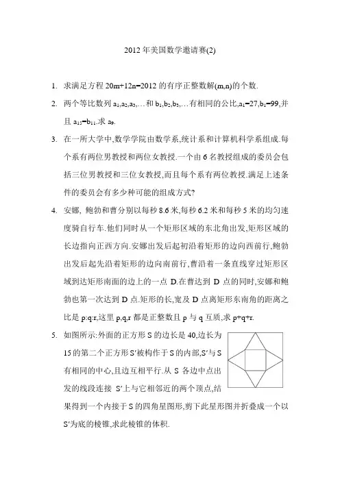
2012年美国数学邀请赛(2)1.求满足方程20m+12n=2012的有序正整数解(m,n)的个数.2.两个等比数列a1,a2,a3,⋯和b1,b2,b3,⋯有相同的公比,a1=27,b1=99,并且a15=b11.求a9.3.在一所大学中,数学学院由数学系,统计系和计算机科学系组成.每个系有两位男教授和两位女教授.一个由6名教授组成的委员会包括三位男教授和三位女教授,而且每个系有两位教授.满足上述条件的委员会有多少种可能的组成方式?4.安娜, 鲍勃和曹分别以每秒8.6米,每秒6.2米和每秒5米的均匀速度骑自行车.他们同时从一个矩形区域的东北角出发,矩形区域的长边指向正西方向.安娜出发后起初沿着矩形的边向西前行,鲍勃出发后起先沿着矩形的边向南前行,曹沿着一条直线穿过矩形区域到达矩形南面的边上的一点D.在曹达到D点的同时,安娜和鲍勃也第一次达到D点.矩形的长,宽及D点离矩形东南角的距离之比是p:q:r,这里p,q,r都是正整数且p与q互质,求p+q+r.5.如图所示:外面的正方形S的边长是40,边长为15的第二个正方形S'被构作于S的内部,S'与S有相同的中心,且边互相平行.从S各边中点出发的线段连接S'上与它相邻近的两个顶点,结果得到一个内接于S的四角星图形,剪下此星形图并折叠成一个以S'为底的棱锥,求此棱锥的体积.6. 令复数z=a+bi 有|z|=5,b>0,且使得(1+2i)z 3与z 5之间的距离达到最大,设z 4=c+di,求c+d.7. 令S 是一个递增的正整数数列,其中的每一个数用二进制表达时恰好有8个1,令N 是S 中的第1000个数,求N 被1000除的余数.8. 复数z 和w 满足z+w i 20=5+i,w+z i 12=-4+10i.求|zw|的最小值. 9. 实数x 和y 满足y sin x sin =3,y cos x cos =21,y 2sin x 2sin +y 2cos x 2cos 的值可以写成q p ,这里p 和q 是互质的正整数,求p+q.10. 已知n 是不大于1000的正整数,且存在一个正实数x,使得n=x[x],这样的n 有多少个?(注:[x]表示不大于x 的最大整数)11. 令f 1(x)=32-1x 33+,当n ≥2时,定义f n (x)=f 1(f n-1(x)).满足f 1001(x)=x-3的x 的值可以表示成nm ,这里m 和n 是互质的正整数,求m+n. 12. 对一个正整数p,如果n 与p 的任何一个倍数的差的绝对值都大于2,则定义正整数n 为“p -稳定数”.例如:“10-稳定数”的集合是{3,4,5,6,7,13,14,15,16,17,23,⋯}.求所有不超过10000且同时为“7-稳定数”,“11-稳定数”,“13-稳定数”的正整数的个数.13. 正∆ABC 的边长是111,有四个都与∆ABC 全等的不同的三角形AD 1E 1, AD 1E 2, AD 2E 3和 AD 2E 4,其中BD 1=BD 2=11.求 ∑=41k 2k )CE(.14. 在9个人形成的一个小组中,安排每个人都恰好与小组中的其他两个人握手.N 是可能发生的握手安排方式的种数.两个不同的握手安排,是指当且仅当至少有两个人,他们在某一个安排中握手了,那么他们在另一个安排中不握手.求N被1000除的余数.15.内接于圆ω的∆ABC有AB=5,BC=7,AC=3.∠A的平分线与边BC相交于D,与圆ω的第二个交点是E.设圆γ是以DE为直径的圆,圆ω与m,这里m和n是互质的正整数,求m+n.圆γ的第二个交点是F,AF2=n答案034 363 088 061 750125 032 040 107 496008 958 677 016 919。
1985 年美国大学生数学建模竞赛MCM 试题1985年MCM:动物种群选择合适的鱼类和哺乳动物数据准确模型。
模型动物的自然表达人口水平与环境相互作用的不同群体的环境的重要参数,然后调整账户获取表单模型符合实际的动物提取的方法。
包括任何食物或限制以外的空间限制,得到数据的支持。
考虑所涉及的各种数量的价值,收获数量和人口规模本身,为了设计一个数字量代表的整体价值收获。
找到一个收集政策的人口规模和时间优化的价值收获在很长一段时间。
检查政策优化价值在现实的环境条件。
1985年MCM B:战略储备管理钴、不产生在美国,许多行业至关重要。
(国防占17%的钴生产。
1979年)钴大部分来自非洲中部,一个政治上不稳定的地区。
1946年的战略和关键材料储备法案需要钴储备,将美国政府通过一项为期三年的战争。
建立了库存在1950年代,出售大部分在1970年代初,然后决定在1970年代末建立起来,与8540万磅。
大约一半的库存目标的储备已经在1982年收购了。
建立一个数学模型来管理储备的战略金属钴。
你需要考虑这样的问题:库存应该有多大?以什么速度应该被收购?一个合理的代价是什么金属?你也要考虑这样的问题:什么时候库存应该画下来吗?以什么速度应该是画下来吗?在金属价格是合理出售什么?它应该如何分配?有用的信息在钴政府计划在2500万年需要2500万磅的钴。
美国大约有1亿磅的钴矿床。
生产变得经济可行当价格达到22美元/磅(如发生在1981年)。
要花四年滚动操作,和thsn六百万英镑每年可以生产。
1980年,120万磅的钴回收,总消费的7%。
1986 年美国大学生数学建模竞赛MCM 试题1986年MCM A:水文数据下表给出了Z的水深度尺表面点的直角坐标X,Y在码(14数据点表省略)。
深度测量在退潮。
你的船有一个五英尺的草案。
你应该避免什么地区内的矩形(75200)X(-50、150)?1986年MCM B:Emergency-Facilities位置迄今为止,力拓的乡牧场没有自己的应急设施。
2012 Contest ProblemsMCM PROBLEMSPROBLEM A: The Leaves of a Tree"How much do the leaves on a tree weigh?" How might one estimate the actual weight of the leaves (or for that matter any other parts of the tree)? How might one classify leaves? Build a mathematical model to describe and classify leaves. Consider and answer the following:• Why do leaves have the various shapes that they have?• Do the shapes “minimize” overlapping individual shadows that are cast, so as to maximize exposure? Does the distribution of leaves within the “volume” of the tree and its branches effect the shape?• Speaking of profiles, is leaf shape (general characteristics) related to tree profile/branching structure?• How would you estimate the leaf mass of a tree? Is there a correlation between the leaf mass and the size characteristics of the tree (height, mass, volume defined by the profile)?In addition to your one page summary sheet prepare a one page letter to an editor of a scientific journal outlining your key findings.“一棵树的叶子有多重?”怎么能估计树的叶子(或者树的任何其它部分)的实际重量?怎样对叶子进行分类?建立一个数学模型来对叶子进行描述和分类。
2012年美国大学生数学建模竞赛A题题目翻译:一棵树的叶子。
一棵树的叶子有多重?怎么能估计树的叶子(或者树的任何其它部分)的实际重量?怎样对叶子进行分类?建立一个数学模型来对叶子进行描述和分类。
摘要我们构建了四个模型来研究叶的分类,叶子形状和叶片分布之间的关系,叶子的形状和树的轮廓的关联,以及一棵树的树叶总质量。
模型1处理叶的分类。
我们主要侧重于最显着的叶片的特征,即,形状。
我们创建七个几何参数以量化叶的形状。
然后,我们选择了六种常见的类型的叶子构造一个数据库。
通过计算的样品的与这些典型叶子的偏差指数,我们可以将叶子进行分类。
为了说明这个分类过程中,我们使用了枫叶作为测试。
模型2研究叶的形状和叶片分布之间的关系。
首先,我们将一棵树化为理想模型,然后介绍太阳高度的概念。
通过考虑叶片长度和节间在不同太阳高度下的关系,分析重叠的片叶阴影,我们发现树叶的形状和分布随着太阳高度进行优化以最大化接受阳光照射。
我们将该模型应用到三类试验树木。
模型3讨论树的轮廓和叶的形状之间可能存在关联。
基于叶脉和树的分支结构的相似性,我们认为,叶子的形状在二维上相似于一个树的轮廓。
采用模型1的方法,我们设置了几个参数来反映每棵树的大概形状,并通过它们的叶子将其进行比较。
在统计工具的帮助下,我们展示了一个树的轮廓与其叶子形状之间的粗略的关联。
模型4通那过给定的树的大小特征,估计了一棵树叶子的总质量。
并引入固碳率和树龄来建立叶的总质量和树的大小之间的联系。
由于单位质量的一个叶以一个恒等的速率固碳,固碳率与树龄之间是一个二次关系,并且树的年龄关系经历逻辑斯蒂增长。
介绍:我们解决四个主要子问题:•分类的叶子,•叶分布和叶片形状之间的关系,•树的轮廓和叶的形状的关系,和•一棵树叶片总质量的计算。
要解决的第一个问题,我们选择一组参数来量化叶片的形状特征和使用叶的形状作为我们的分类过程的主要标准。
对于第二个问题,由于叶子的形状影响着叶之间的重叠,我们将一片叶子直接投射到它下面的一片叶子的阴影重叠区域作为叶片分布和叶片形状之间的一个联系,我们假设叶片分布总是趋于尽量减少重叠的区域。
星际犯罪塑型(ICM)正在调查串谋犯犯罪行为。
调查是非常有信心,他们知道的几名成员的阴谋,但他们进行逮捕之前,希望能找出其他成员和领导人。
阴谋和所有可能涉嫌同谋为同一家公司在一个大办公室复杂的工作。
“公司一直快速增长,并为自己的名称,开发和销售计算机银行和信用卡公司的软件。
ICM最近发现了一个消息从一个小集组82个工人,他们认为在公司将帮助他们找到最有可能的候选人身份不明的同谋者和未知的领导人。
由于信息流量是所有的办公在该公司的工人,它很可能是一些(或许很多)在确定的传播者消息流量不涉及阴谋。
事实上,他们是一定的,他们知道有些人谁是不是在阴谋。
建模工作的目标将是确定人们在办公室复杂谁是最有可能的同谋。
一个优先列表将是理想的,因此ICM可以调查,监视之下的地方,和/或询问最有可能的候选人。
一个判别线分离从非同谋的同谋也将是有益的,以明显的分类,在每个人组。
这也将是有用的模型,如果提名的阴谋领导人检察官办公室。
在当前情况下的数据是给你的犯罪建模团队,你的上司给你以下情形(称为调查的EZ),她曾在几年前在另一座城市。
甚至虽然她是她对简易案件的工作感到非常自豪,她说,这是一个非常小的,简单的例子,但它可以帮助你了解自己的任务。
她的数据如下:她考虑为同谋的十人分别为:安妮#,鲍勃,卡罗尔,大卫*,艾伦,弗雷德,乔治·哈利,伊内兹和JAYE#的。
(*表示已知的同谋者,#表示事先已知nonconspirators)28消息,她为她的案件有编号为每个主题年表的消息,她分配的基础上分析她的消息:安妮对鲍勃:你为什么今天迟到了吗?(1)鲍勃对卡罗尔:这该死的安妮总是看着我。
我是不是晚了。
(1)卡罗尔对戴夫:安娜和鲍勃再次战斗是鲍勃的迟到。
(1)戴夫对艾伦:我要看看你今天早晨。
当你能来吗?带来的预算文件。
(2)戴夫对弗雷德:我能来,随时随地今天看到你。
让我知道什么时候是一个好时机。
我应该带来的预算文件吗?(2)戴夫对乔治:我会看到你以后---说不完的话。
2000到2012年AMC10美国数学竞赛0 0P 0 A 0 B 0 C 0D 0 全美中学数学分级能力测验(AMC 10)2000年 第01届 美国AMC10 (2000年2月 日 时间75分钟)1. 国际数学奥林匹亚将于2001年在美国举办,假设I 、M 、O 分别表示不同的正整数,且满足I ⨯M ⨯O =2001,则试问I +M +O 之最大值为 。
(A) 23 (B) 55 (C) 99 (D) 111 (E) 6712. 2000(20002000)为 。
(A) 20002001 (B) 40002000 (C) 20004000 (D) 40000002000 (E) 200040000003. Jenny 每天早上都会吃掉她所剩下的聪明豆的20%,今知在第二天结束时,有32颗剩下,试问一开始聪明豆有 颗。
(A) 40 (B) 50 (C) 55 (D) 60 (E) 754. Candra 每月要付给网络公司固定的月租费及上网的拨接费,已知她12月的账单为12.48元,而她1月的账单为17.54元,若她1月的上网时间是12月的两倍,试问月租费是 元。
(A) 2.53 (B) 5.06 (C) 6.24 (D) 7.42 (E) 8.775. 如图M ,N 分别为PA 与PB 之中点,试问当P 在一条平行AB 的直 在线移动时,下列各数值有 项会变动。
(a) MN 长 (b) △P AB 之周长 (c) △P AB 之面积 (d) ABNM 之面积(A) 0项 (B) 1项 (C) 2项 (D) 3项 (E) 4项 6. 费氏数列是以两个1开始,接下来各项均为前两项之和,试问在费氏数列各项的个位数字中, 最后出现的阿拉伯数字为 。
(A) 0 (B) 4 (C) 6 (D) 7 (E) 97. 如图,矩形ABCD 中,AD =1,P 在AB 上,且DP 与DB 三等分∠ADC ,试问△BDP 之周长为 。
2000到2012年A M C10美国数学竞赛全美中学数学分级能力测验(AMC 10)2000年 第01届 美国AMC10 (2000年2月 日 时间75分钟)1. 国际数学奥林匹亚将于2001年在美国举办,假设I 、M 、O 分别表示不同的正整数,且满足I ?M ?O =2001,则试问I ?M ?O 之最大值为 。
(A) 23 (B) 55 (C) 99 (D) 111 (E) 6712. 2000(20002000)为 。
(A) 20002001 (B) 40002000 (C) 20004000 (D) 40000002000 (E) 200040000003. Jenny 每天早上都会吃掉她所剩下的聪明豆的20%,今知在第二天结束时,有32颗剩下,试问一开始聪明豆有 颗。
754. Candra 她12月的账单为12.48元,而她1月的账单为17.54元,若她1月的上网时间是12月的两倍,试问月租费是 元。
(A) 2.53 (B) 5.06 (C) 6.24 (D) 7.42 (E) 8.775. 如图M ,N 分别为PA 与PB 之中点,试问当P 在一条平行AB 的直 在线移动时,下列各数值有 项会变动。
(a) MN 长 (b) △PAB 之周长 (c) △PAB 之面积 (d) ABNM 之面积(A) 0项 (B) 1项 (C) 2项 (D) 3项 (E) 4项6. 费氏数列是以两个1开始,接下来各项均为前两项之和,试问在P 0 A 0B 0C 0D 图3图2 图1 图0 费氏数列各项的个位数字中, 最后出现的阿拉伯数字为 。
(A) 0 (B) 4 (C) 6 (D) 7 (E) 97. 如图,矩形ABCD 中,AD =1,P 在AB 上,且DP 与DB 三等分 ?ADC ,试问△BDP 之周长为 。
(A) 3?33(B) 2?334 (C) 2?2 (D) 2533+ (E) 2?3358. 在奥林匹克高中,有52的新生与54的高二生参加AMC 10年级测验。
IMPORTANT CHANGE TO CONTEST RULES FOR MCM/ICM 2012:
2012年MCM/ICM的竞赛规则的重大变化:
Teams (Student or Advisor) are now required to submit an electronic copy (summary sheet and solution) of their solution paper by email to solutions@. Your email MUST be received at COMAP by the submission deadline of 8:00 PM EST, February 13, 2012. Teams are free to choose between MCM Problem A, MCM Problem B or ICM Problem C.
团队(学生或指导老师)必须将解决方案文件的电子副本(汇总表及解决方案)以电子邮件的形式发送到solutions@。
你们的电子邮件必须在美国东部时间2012年2月13日之前发送到COMAP。
团队可以自由选择MCM中的A、B题或ICM中的C题。
COMAP Mirror Site: For more in:
/undergraduate/contests/mcm/
COMAP是镜像网站:欲了解更多:
/undergraduate/contests/mcm/
MCM: The Mathematical Contest in Modeling
MCM:数学建模竞赛
ICM: The Interdisciplinary Contest in Modeling
ICM的:交叉学科建模竞赛
2012 Contest Problems
MCM PROBLEMS
PROBLEM A: The Leaves of a Tree
一个树的叶子
"How much do the leaves on a tree weigh?" How might one estimate the actual weight of the leaves (or for that matter any other parts of the tree)? How might one classify leaves? Build a mathematical model to describe and classify leaves. Consider and answer the following:
“一颗树上的叶子有多重?”如何估计这些叶子(或者一颗树的任何其他部分)的实际重量?又如何分类这些叶子?建立一个数学模型来描述和分类叶子。
考虑并回答下列问题:
• Why do leaves have the various shapes that they have?
为什么叶子有各种形状?
• Do the shapes “minimize” overlapping individual shadows that are cast, so as to maximize exposure? Does the distribution of leaves within the “volume” of the tree and its branches effect the shape?
这些叶子形状是以最小化来重叠自身阴影或者说是最大化来曝光吗?树叶“量”上的分布和树的分支影响了树叶的形状吗?
• Speaking of profiles, is leaf shape (general characteristics) related to tree profile/branching structure?
就树型而言,叶子的形状(一般特征)和树型/分支结构有关吗?
• How would you estimate the leaf mass of a tree? Is there a correlation between the leaf mass and the size characteristics of the tree (height, mass, volume defined by the profile)?
你将如何估计一棵树的叶质量?在树叶质量和树的大小特性(高度、重量或者体积)之间有一个关系吗?
In addition to your one page summary sheet prepare a one page letter to an editor of a scientific journal outlining your key findings.。