Diversity-Multiplexing-Delay Tradeoff in Selection Cooperation Networks with ARQ

A New Algorithm for Channel Estimation Based on Pilot-aided and EM in Software RadioOFDM SystemWU DingxueInstitute for Pattern Recognition and Artificial Intelligence, Huazhong University of Science and Technology, Wuhan 430076, China Computer Department,Huanggang Normal UniversityHuangGang City , ChinaE-mail:jsjwdx@Tian JinwenInstitute for Pattern Recognition and Artificial Intelligence, Huazhong University of Science and Technology, Wuhan 430076, Chinawudingxue@Abstract—In order to increase the transmission efficiency of OFDM system, considering the special structure of Software Radio OFDM system, this paper proposes gradient acceleration method of EM algorithm(▽-EM) for OFDM systems channel estimation with Pilot assisted symbol modulation expectation. The simulation result shows that the new method can reduce the complexity and iteration times, andit has also still lower BER compared to traditional method.Keywords- OFDM system, pilot , channel estimation , ▽-EM algorithm， software radioI.I NTRODUCTIONA Software-Defined Radio (SDR) system is a radio communication system where components that have typically been implemented in hardware (i.e. mixers, filters, amplifiers, modulators/demodulators,detectors. etc.)are instead implemented using software on a personal computer or other embedded computing devices. O rthogonal frequency-division multiplexing (OFDM), which can transform a frequency-selective fading channel into many parallel flat fading subchannels, is an efficient technique to combat multipath delay spread in high-rate wireless systems, especially CDMA system.The wireless systems combining OFDM and CDMA based on Software Radio will bring on a strong competitiveness, OFDM-CDMA based on Software Radio is called Software Radio OFDM system. In the coherent demodulation of OFDM system, the accurate estimation of channel is one of the key techniques to improve system performance.Software Radio OFDM channel estimation methods generally can be classified into two categories: one is the channel estimation method based on pilot; the other is blind channel estimation method. The former one consists of two steps: (1) collect the channel fading coefficients in pilot subcarrier; (2) interpolate the collected fading coefficients or conduct a fitting or approximation on the fading coefficients using its responding function of channel frequency domain.In wideband mobile channels, the pilot-symbol-aided channel estimation scheme has been proven tobe a feasible method for OFDM system1. Channelestimation techniques based pilot symbol arrangement inOFDM systems have been analyzed in2, there have manymethod, including linear, cubic interpolation, matched filter 2,6, radial basis function(RBF),and EM algorithm4,5, the best performance is EM combined with other method, such asspace-altering generalized EM method (SAGE)3, buttraditional EM algorithm has a big deficiency, itconvergences very slow, and has high complexity.We proposed a new way to reduced the complexity of the EM algorithm and accelerate the convergence in this paper, i.e the gradient EM algorithm(▽-EM), although a little performance degraded compared to Perfect CIR, but it is much better that the tradition methods(such as cubic interpolation) are. And it has fast convergence rate than Perfect CIR, It is a good tradeoff between bit error rate (BER) and rapidity.II.A MATHEMATICS MODELS OF SOFTWARE RADIO INOFDM-CDMA COMMUNICATIONS S YSTEM RECEIVERIn modern military communications, OFDM-CDMAcommunications become more and more important. It iswidely used in various strategical and tacticalcommunications, command and control, and intelligence delivering systems. However, for the present, spread spectrum communications system, the digitalization and software realization degree is very low. Considering that the key part of spread spectrum communications system is its receiving system, we realize a typical OFDM-CDMA communications system based on software radio, see Fig. 1.978-0-7695-3522-7/09 $25.00 © 2009 IEEE2009 International Conference on Communication Software and Networks DOI 10.1109/ICCSN.2009.100341III. C HANNEL ESTIMATION MODEL B ASED ON P ILOT -AIDED IN S OFTWARE R ADIO OFDM S YSTEMChannel estimation mode based on pilot-aided in software radio OFDM system is showed as Figure.2.Assume the number of subcarriers in Software Radio OFDM system is N, among which M subcarriers are usedfor transmit pilot symbol vector, noted as 1M × vector P .The binary code stream produced in information source ofsystem transmitting end is devided into N-M d =N parallel data streams. Each data stream is digitallymodulated through QPSK and becomes transmission datasymbol vector, noted as 1D N × vector n D . Pilot isinserted so that frequency domain sending data n S isproduced, which is send to IFFT module to be modulated.Insert cyclic prefix (CP) into the modulated data to convertit into the serial data to be send. After removing the CP ofthe receiving data in the receiving end, it is called FFT, andit becomes frequency domain receiving data n Y . Assumethe length of CP is bigger than channel impulse response length, then there is no ISI and ICI in the system. The relation between the nth receiving symbol and sending symbol in the Software Radio OFDM system is:()()()()n n n n Y k H k S k W k =+,0,1,,1k N =−" （1）The matrix expression is: (0)(0)(0)(1)(1)(1)(1)(1)(1)n n n n n n n n n Y S H Y S H Y N S N H N ⎡⎤⎡⎤⎡⎤⎢⎥⎢⎥⎢⎥⎢⎥⎢⎥⎢⎥=⎢⎥⎢⎥⎢⎥⎢⎥⎢⎥⎢⎥−−−⎣⎦⎣⎦⎣⎦#%#Simplified as:()n n n n Diag =+Y S H W （2）To simplify for later illustration, the index n is omitted, thus it is expressed as:()Diag =+Y S H W ()L Diag =+S F h W （3）Where ()Diag S refers to a diagonal matrix which takes each element of vector S as its diagonal element. W is an independent simultaneous distribution Gauss white noise vector. Assume the channel doesn’t change during anOFDM symbol cycle,[(0)(1)(1)]Th h h L =−h "is the channel impulseresponse and L is the length of the impulse response. ()H k is the fading coefficient of the kth subcarrier, 210()()L j kl Nl H k h l e π−−==∑,0,1,,1k N =−". Where L F is a submatrix of the descrete Fourier transformation matrix Figure 1. A mathematics models of software radio in OFDM-CDMA communications system receiverFigure 2. Channel estimation model based on pilot-aided in Software Radio OFDM systemof point N after the bottom N L − columns are removed. Where []2,j klN L k l e π−=F , 0,1,,1k N =−", 0,1,,1l L =−".Generally, pilot is inserted into data of the same interral f D and a complete ODFM sending symbol S is got:()()f S k S mD l =+()0((1))1f f P m l D m D l l D =⎧=⎨−+−⎩"=1,, （4）Define 1N × variable d()()f d k d mD l =+ 00((1))1f f l D m D l l D =⎧=⎨−+−⎩"=1,, （5）IV. GRADIENT EM ALGORITHM (▽-EM) B ASED ONP ILOT Assume the size of constellation map is C (4,QPSK) after the sending binary data stream is modulated through QPSK. The symbol in the constellation map is noted as ,1,2,,l q l C =".If h is given, the (,|)f Y d h can be taken as joint condition probability density function of intact data (),Y d . Suppose the channel doesn’t change during anOFDM symbol cycle, and the receiving data of Nsubcarriers are independent, then (,|)f Y d h 1((),()|())N Y k f Y k S k H k −==∏Where((),()|())Y f Y k S k Hk 22()()())2WY k S k H k σ−=−EM iteration algotithm is completed through thefollowing two steps:E-step: {}()()(|)log (,|)|,p p Q E f ′=h h Y d h h Y （6） M-step:(1)()arg max((|))p p Q +′=hhh h （7）That is, give the channel estimation value and receiving data of the pth iteration, get expectation value of (,|)f Y d h about d . The number h which can make the expectation value be the maximum one is the channel estimation value of the next iteration. In formula (5), thedistribution of d and channel parameter h are independentfrom each other, and log (,|)f Y d h log (|,)log (|)f f =+Y h d d h , so to get the conditional expectation of log (,|)f Y d h can be simplified as to determine the conditional expectation of log (|,)f Y h d . It is showed asthe following formula:{}()log (|,)|,p E f Y h d h Y()()21()exp(|,2p N n nD E σ⎧⎫⎪⎪=−⎨⎬⎪⎪⎩⎭h,Y,d h Y{}()21)()|,2p W WN E D σ=−−h,Y ,d h Y （8）Where()D h,Y,d 2()L diag =−Y S F h12()()()N k Y k S k H k −==−∑。

交叉滞后自由估计模型摘要：一、交叉滞后自由估计模型的简介二、交叉滞后自由估计模型的基本原理三、交叉滞后自由估计模型的应用领域四、交叉滞后自由估计模型的优缺点分析五、结论正文：交叉滞后自由估计模型是一种用于分析时间序列数据之间相关性的统计模型，特别是在处理面板数据时具有重要作用。

该模型在经济学、金融学、社会学等多个学科领域都有广泛应用。

交叉滞后自由估计模型的基本原理是通过构建多个滞后阶数不同的自回归模型，并使用最大似然估计方法来估计参数。

这种方法不仅考虑了数据之间的相关性，还允许研究者根据实际问题灵活选择合适的滞后阶数。

交叉滞后自由估计模型在以下领域中具有广泛应用：1.宏观经济学：用于分析不同国家或地区之间的经济增长、通货膨胀、利率等变量之间的关系。

2.金融学：用于研究股票、债券、汇率等金融变量之间的联动性，以及金融市场的风险传染。

3.社会学：用于探讨不同社会群体之间的互动、文化传播、生活习惯等现象。

4.环境科学：用于研究气候变化、生态系统、污染物排放等跨区域、跨时间的相关性。

交叉滞后自由估计模型具有以下优缺点：优点：1.模型具有较强的稳健性，能够处理不同滞后阶数的相关性问题。

2.允许研究者根据实际问题灵活选择合适的滞后阶数，提高了模型的实用性。

3.可以应用于多种学科领域，具有广泛的应用价值。

缺点：1.模型参数估计可能受到多重共线性问题的影响，导致参数估计不准确。

2.当滞后阶数较多时，模型的计算复杂度较高，可能需要较长时间来完成估计过程。

总的来说，交叉滞后自由估计模型是一种功能强大的统计分析方法，适用于处理各种复杂的相关性问题。

AgilentDigital Modulation in Communications Systems—An IntroductionApplication Note 1298This application note introduces the concepts of digital modulation used in many communications systems today. Emphasis is placed on explaining the tradeoffs that are made to optimize efficiencies in system design.Most communications systems fall into one of three categories: bandwidth efficient, power efficient, or cost efficient. Bandwidth efficiency describes the ability of a modulation scheme to accommodate data within a limited bandwidth. Power efficiency describes the ability of the system to reliably send information at the lowest practical power level.In most systems, there is a high priority on band-width efficiency. The parameter to be optimized depends on the demands of the particular system, as can be seen in the following two examples.For designers of digital terrestrial microwave radios, their highest priority is good bandwidth efficiency with low bit-error-rate. They have plenty of power available and are not concerned with power efficiency. They are not especially con-cerned with receiver cost or complexity because they do not have to build large numbers of them. On the other hand, designers of hand-held cellular phones put a high priority on power efficiency because these phones need to run on a battery. Cost is also a high priority because cellular phones must be low-cost to encourage more users. Accord-ingly, these systems sacrifice some bandwidth efficiency to get power and cost efficiency. Every time one of these efficiency parameters (bandwidth, power, or cost) is increased, another one decreases, becomes more complex, or does not perform well in a poor environment. Cost is a dom-inant system priority. Low-cost radios will always be in demand. In the past, it was possible to make a radio low-cost by sacrificing power and band-width efficiency. This is no longer possible. The radio spectrum is very valuable and operators who do not use the spectrum efficiently could lose their existing licenses or lose out in the competition for new ones. These are the tradeoffs that must be considered in digital RF communications design. This application note covers•the reasons for the move to digital modulation;•how information is modulated onto in-phase (I) and quadrature (Q) signals;•different types of digital modulation;•filtering techniques to conserve bandwidth; •ways of looking at digitally modulated signals;•multiplexing techniques used to share the transmission channel;•how a digital transmitter and receiver work;•measurements on digital RF communications systems;•an overview table with key specifications for the major digital communications systems; and •a glossary of terms used in digital RF communi-cations.These concepts form the building blocks of any communications system. If you understand the building blocks, then you will be able to under-stand how any communications system, present or future, works.Introduction25 5 677 7 8 8 9 10 10 1112 12 12 13 14 14 15 15 16 17 18 19 20 21 22 22 23 23 24 25 26 27 28 29 29 30 311. Why Digital Modulation?1.1 Trading off simplicity and bandwidth1.2 Industry trends2. Using I/Q Modulation (Amplitude and Phase Control) to Convey Information2.1 Transmitting information2.2 Signal characteristics that can be modified2.3 Polar display—magnitude and phase representedtogether2.4 Signal changes or modifications in polar form2.5 I/Q formats2.6 I and Q in a radio transmitter2.7 I and Q in a radio receiver2.8 Why use I and Q?3. Digital Modulation Types and Relative Efficiencies3.1 Applications3.1.1 Bit rate and symbol rate3.1.2 Spectrum (bandwidth) requirements3.1.3 Symbol clock3.2 Phase Shift Keying (PSK)3.3 Frequency Shift Keying3.4 Minimum Shift Keying (MSK)3.5 Quadrature Amplitude Modulation (QAM)3.6 Theoretical bandwidth efficiency limits3.7 Spectral efficiency examples in practical radios3.8 I/Q offset modulation3.9 Differential modulation3.10 Constant amplitude modulation4. Filtering4.1 Nyquist or raised cosine filter4.2 Transmitter-receiver matched filters4.3 Gaussian filter4.4 Filter bandwidth parameter alpha4.5 Filter bandwidth effects4.6 Chebyshev equiripple FIR (finite impulse response) filter4.7 Spectral efficiency versus power consumption5. Different Ways of Looking at a Digitally Modulated Signal Time and Frequency Domain View5.1 Power and frequency view5.2 Constellation diagrams5.3 Eye diagrams5.4 Trellis diagramsTable of Contents332 32 32 33 33 34 3435 35 3637 37 37 38 38 39 39 39 40 41 41 42 434344466. Sharing the Channel6.1 Multiplexing—frequency6.2 Multiplexing—time6.3 Multiplexing—code6.4 Multiplexing—geography6.5 Combining multiplexing modes6.6 Penetration versus efficiency7. How Digital Transmitters and Receivers Work7.1 A digital communications transmitter7.2 A digital communications receiver8. Measurements on Digital RF Communications Systems 8.1 Power measurements8.1.1 Adjacent Channel Power8.2 Frequency measurements8.2.1 Occupied bandwidth8.3 Timing measurements8.4 Modulation accuracy8.5 Understanding Error Vector Magnitude (EVM)8.6 Troubleshooting with error vector measurements8.7 Magnitude versus phase error8.8 I/Q phase error versus time8.9 Error Vector Magnitude versus time8.10 Error spectrum (EVM versus frequency)9. Summary10. Overview of Communications Systems11. Glossary of TermsTable of Contents (continued)4The move to digital modulation provides more information capacity, compatibility with digital data services, higher data security, better quality communications, and quicker system availability. Developers of communications systems face these constraints:•available bandwidth•permissible power•inherent noise level of the systemThe RF spectrum must be shared, yet every day there are more users for that spectrum as demand for communications services increases. Digital modulation schemes have greater capacity to con-vey large amounts of information than analog mod-ulation schemes. 1.1 Trading off simplicity and bandwidthThere is a fundamental tradeoff in communication systems. Simple hardware can be used in transmit-ters and receivers to communicate information. However, this uses a lot of spectrum which limits the number of users. Alternatively, more complex transmitters and receivers can be used to transmit the same information over less bandwidth. The transition to more and more spectrally efficient transmission techniques requires more and more complex hardware. Complex hardware is difficult to design, test, and build. This tradeoff exists whether communication is over air or wire, analog or digital.Figure 1. The Fundamental Tradeoff1. Why Digital Modulation?51.2 Industry trendsOver the past few years a major transition has occurred from simple analog Amplitude Mod-ulation (AM) and Frequency/Phase Modulation (FM/PM) to new digital modulation techniques. Examples of digital modulation include•QPSK (Quadrature Phase Shift Keying)•FSK (Frequency Shift Keying)•MSK (Minimum Shift Keying)•QAM (Quadrature Amplitude Modulation) Another layer of complexity in many new systems is multiplexing. Two principal types of multiplex-ing (or “multiple access”) are TDMA (Time Division Multiple Access) and CDMA (Code Division Multiple Access). These are two different ways to add diversity to signals allowing different signals to be separated from one another.Figure 2. Trends in the Industry62.1 Transmitting informationTo transmit a signal over the air, there are three main steps:1.A pure carrier is generated at the transmitter.2.The carrier is modulated with the informationto be transmitted. Any reliably detectablechange in signal characteristics can carryinformation.3.At the receiver the signal modifications orchanges are detected and demodulated.2.2 Signal characteristics that can be modified There are only three characteristics of a signal that can be changed over time: amplitude, phase, or fre-quency. However, phase and frequency are just dif-ferent ways to view or measure the same signal change. In AM, the amplitude of a high-frequency carrier signal is varied in proportion to the instantaneous amplitude of the modulating message signal.Frequency Modulation (FM) is the most popular analog modulation technique used in mobile com-munications systems. In FM, the amplitude of the modulating carrier is kept constant while its fre-quency is varied by the modulating message signal.Amplitude and phase can be modulated simultane-ously and separately, but this is difficult to gener-ate, and especially difficult to detect. Instead, in practical systems the signal is separated into another set of independent components: I(In-phase) and Q(Quadrature). These components are orthogonal and do not interfere with each other.Figure 3. Transmitting Information (Analog or Digital)Figure 4. Signal Characteristics to Modify2. Using I/Q Modulation to Convey Information72.3 Polar display—magnitude and phase repre-sented togetherA simple way to view amplitude and phase is with the polar diagram. The carrier becomes a frequency and phase reference and the signal is interpreted relative to the carrier. The signal can be expressed in polar form as a magnitude and a phase. The phase is relative to a reference signal, the carrier in most communication systems. The magnitude is either an absolute or relative value. Both are used in digital communication systems. Polar diagrams are the basis of many displays used in digital com-munications, although it is common to describe the signal vector by its rectangular coordinates of I (In-phase) and Q(Quadrature).2.4 Signal changes or modifications inpolar formFigure 6 shows different forms of modulation in polar form. Magnitude is represented as the dis-tance from the center and phase is represented as the angle.Amplitude modulation (AM) changes only the magnitude of the signal. Phase modulation (PM) changes only the phase of the signal. Amplitude and phase modulation can be used together. Frequency modulation (FM) looks similar to phase modulation, though frequency is the controlled parameter, rather than relative phase.Figure 6. Signal Changes or Modifications8One example of the difficulties in RF design can be illustrated with simple amplitude modulation. Generating AM with no associated angular modula-tion should result in a straight line on a polar display. This line should run from the origin to some peak radius or amplitude value. In practice, however, the line is not straight. The amplitude modulation itself often can cause a small amount of unwanted phase modulation. The result is a curved line. It could also be a loop if there is any hysteresis in the system transfer function. Some amount of this distortion is inevitable in any sys-tem where modulation causes amplitude changes. Therefore, the degree of effective amplitude modu-lation in a system will affect some distortion parameters.2.5 I/Q formatsIn digital communications, modulation is often expressed in terms of I and Q. This is a rectangular representation of the polar diagram. On a polar diagram, the I axis lies on the zero degree phase reference, and the Q axis is rotated by 90 degrees. The signal vector’s projection onto the I axis is its “I” component and the projection onto the Q axisis its “Q” component.Figure 7. “I-Q” Format92.6 I and Q in a radio transmitterI/Q diagrams are particularly useful because they mirror the way most digital communications sig-nals are created using an I/Q modulator. In the transmitter, I and Q signals are mixed with the same local oscillator (LO). A 90 degree phase shifter is placed in one of the LO paths. Signals that are separated by 90 degrees are also known as being orthogonal to each other or in quadrature. Signals that are in quadrature do not interfere with each other. They are two independent compo-nents of the signal. When recombined, they are summed to a composite output signal. There are two independent signals in I and Q that can be sent and received with simple circuits. This simpli-fies the design of digital radios. The main advan-tage of I/Q modulation is the symmetric ease of combining independent signal components into a single composite signal and later splitting such a composite signal into its independent component parts. 2.7 I and Q in a radio receiverThe composite signal with magnitude and phase (or I and Q) information arrives at the receiver input. The input signal is mixed with the local oscillator signal at the carrier frequency in two forms. One is at an arbitrary zero phase. The other has a 90 degree phase shift. The composite input signal (in terms of magnitude and phase) is thus broken into an in-phase, I, and a quadrature, Q, component. These two components of the signal are independent and orthogonal. One can be changed without affecting the other. Normally, information cannot be plotted in a polar format and reinterpreted as rectangular values without doing a polar-to-rectangular conversion. This con-version is exactly what is done by the in-phase and quadrature mixing processes in a digital radio. A local oscillator, phase shifter, and two mixers can perform the conversion accurately and efficiently.Figure 8. I and Q in a Practical Radio Transmitter Figure 9. I and Q in a Radio Receiver102.8 Why use I and Q?Digital modulation is easy to accomplish with I/Q modulators. Most digital modulation maps the data to a number of discrete points on the I/Q plane. These are known as constellation points. As the sig-nal moves from one point to another, simultaneous amplitude and phase modulation usually results. To accomplish this with an amplitude modulator and a phase modulator is difficult and complex. It is also impossible with a conventional phase modu-lator. The signal may, in principle, circle the origin in one direction forever, necessitating infinite phase shifting capability. Alternatively, simultaneous AM and Phase Modulation is easy with an I/Q modulator. The I and Q control signals are bounded, but infi-nite phase wrap is possible by properly phasing the I and Q signals.This section covers the main digital modulation formats, their main applications, relative spectral efficiencies, and some variations of the main modulation types as used in practical systems. Fortunately, there are a limited number of modula-tion types which form the building blocks of any system.3.1 ApplicationsThe table below covers the applications for differ-ent modulation formats in both wireless communi-cations and video. Although this note focuses on wireless communica-tions, video applications have also been included in the table for completeness and because of their similarity to other wireless communications.3.1.1 Bit rate and symbol rateTo understand and compare different modulation format efficiencies, it is important to first under-stand the difference between bit rate and symbol rate. The signal bandwidth for the communications channel needed depends on the symbol rate, not on the bit rate.Symbol rate =bit ratethe number of bits transmitted with each symbol 3. Digital Modulation Types and Relative EfficienciesBit rate is the frequency of a system bit stream. Take, for example, a radio with an 8 bit sampler, sampling at 10 kHz for voice. The bit rate, the basic bit stream rate in the radio, would be eight bits multiplied by 10K samples per second, or 80 Kbits per second. (For the moment we will ignore the extra bits required for synchronization, error correction, etc.)Figure 10 is an example of a state diagram of a Quadrature Phase Shift Keying (QPSK) signal. The states can be mapped to zeros and ones. This is a common mapping, but it is not the only one. Any mapping can be used.The symbol rate is the bit rate divided by the num-ber of bits that can be transmitted with each sym-bol. If one bit is transmitted per symbol, as with BPSK, then the symbol rate would be the same as the bit rate of 80 Kbits per second. If two bits are transmitted per symbol, as in QPSK, then the sym-bol rate would be half of the bit rate or 40 Kbits per second. Symbol rate is sometimes called baud rate. Note that baud rate is not the same as bit rate. These terms are often confused. If more bits can be sent with each symbol, then the same amount of data can be sent in a narrower spec-trum. This is why modulation formats that are more complex and use a higher number of states can send the same information over a narrower piece of the RF spectrum.3.1.2 Spectrum (bandwidth) requirementsAn example of how symbol rate influences spec-trum requirements can be seen in eight-state Phase Shift Keying (8PSK). It is a variation of PSK. There are eight possible states that the signal can transi-tion to at any time. The phase of the signal can take any of eight values at any symbol time. Since 23= 8, there are three bits per symbol. This means the symbol rate is one third of the bit rate. This is relatively easy to decode.Figure 10. Bit Rate and Symbol Rate Figure 11. Spectrum Requirements3.1.3 Symbol ClockThe symbol clock represents the frequency and exact timing of the transmission of the individual symbols. At the symbol clock transitions, the trans-mitted carrier is at the correct I/Q(or magnitude/ phase) value to represent a specific symbol (a specific point in the constellation).3.2 Phase Shift KeyingOne of the simplest forms of digital modulation is binary or Bi-Phase Shift Keying (BPSK). One appli-cation where this is used is for deep space teleme-try. The phase of a constant amplitude carrier sig-nal moves between zero and 180 degrees. On an I and Q diagram, the I state has two different values. There are two possible locations in the state dia-gram, so a binary one or zero can be sent. The symbol rate is one bit per symbol.A more common type of phase modulation is Quadrature Phase Shift Keying (QPSK). It is used extensively in applications including CDMA (Code Division Multiple Access) cellular service, wireless local loop, Iridium (a voice/data satellite system) and DVB-S (Digital Video Broadcasting — Satellite). Quadrature means that the signal shifts between phase states which are separated by 90 degrees. The signal shifts in increments of 90 degrees from 45 to 135, –45, or –135 degrees. These points are chosen as they can be easily implemented using an I/Q modulator. Only two I values and two Q values are needed and this gives two bits per symbol. There are four states because 22= 4. It is therefore a more bandwidth-efficient type of modulation than BPSK, potentially twice as efficient.Figure 12. Phase Shift Keying3.3 Frequency Shift KeyingFrequency modulation and phase modulation are closely related. A static frequency shift of +1 Hz means that the phase is constantly advancing at the rate of 360 degrees per second (2 πrad/sec), relative to the phase of the unshifted signal.FSK (Frequency Shift Keying) is used in many applications including cordless and paging sys-tems. Some of the cordless systems include DECT (Digital Enhanced Cordless Telephone) and CT2 (Cordless Telephone 2).In FSK, the frequency of the carrier is changed as a function of the modulating signal (data) being transmitted. Amplitude remains unchanged. In binary FSK (BFSK or 2FSK), a “1” is represented by one frequency and a “0” is represented by another frequency.3.4 Minimum Shift KeyingSince a frequency shift produces an advancing or retarding phase, frequency shifts can be detected by sampling phase at each symbol period. Phase shifts of (2N + 1) π/2radians are easily detected with an I/Q demodulator. At even numbered sym-bols, the polarity of the I channel conveys the transmitted data, while at odd numbered symbols the polarity of the Q channel conveys the data. This orthogonality between I and Q simplifies detection algorithms and hence reduces power con-sumption in a mobile receiver. The minimum fre-quency shift which yields orthogonality of I and Q is that which results in a phase shift of ±π/2radi-ans per symbol (90 degrees per symbol). FSK with this deviation is called MSK (Minimum Shift Keying). The deviation must be accurate in order to generate repeatable 90 degree phase shifts. MSK is used in the GSM (Global System for Mobile Communications) cellular standard. A phase shift of +90 degrees represents a data bit equal to “1,”while –90 degrees represents a “0.” The peak-to-peak frequency shift of an MSK signal is equal to one-half of the bit rate.FSK and MSK produce constant envelope carrier signals, which have no amplitude variations. This is a desirable characteristic for improving the power efficiency of transmitters. Amplitude varia-tions can exercise nonlinearities in an amplifier’s amplitude-transfer function, generating spectral regrowth, a component of adjacent channel power. Therefore, more efficient amplifiers (which tend to be less linear) can be used with constant-envelope signals, reducing power consumption.Figure 13. Frequency Shift KeyingMSK has a narrower spectrum than wider devia-tion forms of FSK. The width of the spectrum is also influenced by the waveforms causing the fre-quency shift. If those waveforms have fast transi-tions or a high slew rate, then the spectrumof the transmitter will be broad. In practice, the waveforms are filtered with a Gaussian filter, resulting in a narrow spectrum. In addition, the Gaussian filter has no time-domain overshoot, which would broaden the spectrum by increasing the peak deviation. MSK with a Gaussian filter is termed GMSK (Gaussian MSK).3.5 Quadrature Amplitude ModulationAnother member of the digital modulation family is Quadrature Amplitude Modulation (QAM). QAM is used in applications including microwave digital radio, DVB-C (Digital Video Broadcasting—Cable), and modems.In 16-state Quadrature Amplitude Modulation (16QAM), there are four I values and four Q values. This results in a total of 16 possible states for the signal. It can transition from any state to any other state at every symbol time. Since 16 = 24, four bits per symbol can be sent. This consists of two bits for I and two bits for Q. The symbol rate is one fourth of the bit rate. So this modulation format produces a more spectrally efficient transmission. It is more efficient than BPSK, QPSK, or 8PSK. Note that QPSK is the same as 4QAM.Another variation is 32QAM. In this case there are six I values and six Q values resulting in a total of 36 possible states (6x6=36). This is too many states for a power of two (the closest power of two is 32). So the four corner symbol states, which take the most power to transmit, are omitted. This reduces the amount of peak power the transmitter has to generate. Since 25= 32, there are five bits per sym-bol and the symbol rate is one fifth of the bit rate. The current practical limits are approximately256QAM, though work is underway to extend the limits to 512 or 1024 QAM. A 256QAM system uses 16 I-values and 16 Q-values, giving 256 possible states. Since 28= 256, each symbol can represent eight bits. A 256QAM signal that can send eight bits per symbol is very spectrally efficient. However, the symbols are very close together and are thus more subject to errors due to noise and distortion. Such a signal may have to be transmit-ted with extra power (to effectively spread the symbols out more) and this reduces power efficiency as compared to simpler schemes.Figure 14. Quadrature Amplitude ModulationCompare the bandwidth efficiency when using256QAM versus BPSK modulation in the radio example in section 3.1.1 (which uses an eight-bit sampler sampling at 10 kHz for voice). BPSK uses80 Ksymbols-per-second sending 1 bit per symbol.A system using 256QAM sends eight bits per sym-bol so the symbol rate would be 10 Ksymbols per second. A 256QAM system enables the same amount of information to be sent as BPSK using only one eighth of the bandwidth. It is eight times more bandwidth efficient. However, there is a tradeoff. The radio becomes more complex and is more susceptible to errors caused by noise and dis-tortion. Error rates of higher-order QAM systems such as this degrade more rapidly than QPSK as noise or interference is introduced. A measureof this degradation would be a higher Bit Error Rate (BER).In any digital modulation system, if the input sig-nal is distorted or severely attenuated the receiver will eventually lose symbol lock completely. If the receiver can no longer recover the symbol clock, it cannot demodulate the signal or recover any infor-mation. With less degradation, the symbol clock can be recovered, but it is noisy, and the symbol locations themselves are noisy. In some cases, a symbol will fall far enough away from its intended position that it will cross over to an adjacent posi-tion. The I and Q level detectors used in the demodulator would misinterpret such a symbol as being in the wrong location, causing bit errors. QPSK is not as efficient, but the states are much farther apart and the system can tolerate a lot more noise before suffering symbol errors. QPSK has no intermediate states between the four corner-symbol locations, so there is less opportunity for the demodulator to misinterpret symbols. QPSK requires less transmitter power than QAM to achieve the same bit error rate.3.6 Theoretical bandwidth efficiency limits Bandwidth efficiency describes how efficiently the allocated bandwidth is utilized or the ability of a modulation scheme to accommodate data, within a limited bandwidth. The table below shows the theoretical bandwidth efficiency limits for the main modulation types. Note that these figures cannot actually be achieved in practical radios since they require perfect modulators, demodula-tors, filter, and transmission paths.If the radio had a perfect (rectangular in the fre-quency domain) filter, then the occupied band-width could be made equal to the symbol rate.Techniques for maximizing spectral efficiency include the following:•Relate the data rate to the frequency shift (as in GSM).•Use premodulation filtering to reduce the occupied bandwidth. Raised cosine filters,as used in NADC, PDC, and PHS, give thebest spectral efficiency.•Restrict the types of transitions.Modulation Theoretical bandwidthformat efficiencylimitsMSK 1bit/second/HzBPSK 1bit/second/HzQPSK 2bits/second/Hz8PSK 3bits/second/Hz16 QAM 4 bits/second/Hz32 QAM 5 bits/second/Hz64 QAM 6 bits/second/Hz256 QAM 8 bits/second/HzEffects of going through the originTake, for example, a QPSK signal where the normalized value changes from 1, 1 to –1, –1. When changing simulta-neously from I and Q values of +1 to I and Q values of –1, the signal trajectory goes through the origin (the I/Q value of 0,0). The origin represents 0 carrier magnitude. A value of 0 magnitude indicates that the carrier amplitude is 0 for a moment.Not all transitions in QPSK result in a trajectory that goes through the origin. If I changes value but Q does not (or vice-versa) the carrier amplitude changes a little, but it does not go through zero. Therefore some symbol transi-tions will result in a small amplitude variation, while others will result in a very large amplitude variation. The clock-recovery circuit in the receiver must deal with this ampli-tude variation uncertainty if it uses amplitude variations to align the receiver clock with the transmitter clock. Spectral regrowth does not automatically result from these trajectories that pass through or near the origin. If the amplifier and associated circuits are perfectly linear, the spectrum (spectral occupancy or occupied bandwidth) will be unchanged. The problem lies in nonlinearities in the circuits.A signal which changes amplitude over a very large range will exercise these nonlinearities to the fullest extent. These nonlinearities will cause distortion products. In con-tinuously modulated systems they will cause “spectral regrowth” or wider modulation sidebands (a phenomenon related to intermodulation distortion). Another term which is sometimes used in this context is “spectral splatter.”However this is a term that is more correctly used in asso-ciation with the increase in the bandwidth of a signal caused by pulsing on and off.3.7 Spectral efficiency examples inpractical radiosThe following examples indicate spectral efficien-cies that are achieved in some practical radio systems.The TDMA version of the North American Digital Cellular (NADC) system, achieves a 48 Kbits-per-second data rate over a 30 kHz bandwidth or 1.6 bits per second per Hz. It is a π/4 DQPSK based system and transmits two bits per symbol. The theoretical efficiency would be two bits per second per Hz and in practice it is 1.6 bits per second per Hz.Another example is a microwave digital radio using 16QAM. This kind of signal is more susceptible to noise and distortion than something simpler such as QPSK. This type of signal is usually sent over a direct line-of-sight microwave link or over a wire where there is very little noise and interference. In this microwave-digital-radio example the bit rate is 140 Mbits per second over a very wide bandwidth of 52.5 MHz. The spectral efficiency is 2.7 bits per second per Hz. To implement this, it takes a very clear line-of-sight transmission path and a precise and optimized high-power transceiver.。

博时量化多因子-概述说明以及解释1.引言1.1 概述引言是一篇文章的开端，它为读者提供了一个整体的背景概述，引起读者的兴趣，并概括地介绍了文章的主题和结构。

本文的主题是博时量化多因子投资策略，下面将对概述部分展开介绍。

在现代投资领域中，投资者通过寻找有效的投资策略来获取更高的收益。

多因子投资策略是一种备受关注的投资方法，它通过综合考虑多个因素来选择和配置投资组合中的个股，以期获得相对于市场整体表现更好的投资回报。

博时量化多因子模型作为博时基金旗下的一种投资策略，采用了先进的量化分析方法，利用大数据和机器学习技术，从众多因子中选择和构建出适用于不同市场环境的投资组合。

它不仅考虑了传统的基本面因素，如估值、盈利能力和成长性等，还结合了技术指标和市场情绪等因素，以提高投资组合的优化效果。

通过博时量化多因子模型，投资者可以更加科学、系统地进行投资决策，提升投资回报的同时，降低风险。

在本文中，将首先介绍多因子投资策略的基本原理和优势，包括为什么多因子投资可以带来超额收益以及如何选择合适的因子。

接着将详细阐述博时量化多因子模型的构建方法和应用实例，分析其在不同市场环境下的表现和优势。

最后，将总结多因子投资的优势，并展望博时量化多因子模型的应用前景。

通过本文的阅读，读者将能够了解到多因子投资策略的基本原理和实施方法，以及博时量化多因子模型在投资领域的应用价值。

希望本文能够为投资者提供一些有价值的思考，帮助他们在投资决策中做出更加明智的选择。

1.2文章结构文章结构：本文分为引言、正文和结论三个部分。

引言部分主要包括概述、文章结构和目的三个方面。

首先，我们将概述本文的主题，即博时量化多因子投资策略，并介绍该策略在投资领域的重要性和研究意义。

其次，我们会具体阐述文章的结构，让读者对整个文章有一个清晰的了解。

最后，我们明确本文的目的，以鼓励读者对该主题进行深入研究，并为实践中的投资决策提供有益的参考。

接下来是正文部分，主要包括多因子投资策略和博时量化多因子模型两个方面。

AbstractMulti-Carrier Modulation is a technique for data-transmission by dividing a high-bit rate data stream is several parallel low bit-rate data streams and using these low bit-rate data streams to modulate several carriers. Multi-Carrier Transmission has a lot of useful properties such as delay-spread tolerance and spectrum efficiency that encourage their use in untethered broadband communications. OFDM is a multi-carrier modulation technique with densely spaced sub-carriers, that has gained a lot of popularity among the broadband community in the last few years. This report is intended to provide a tutorial level introduction to OFDM Modulation, its advantages nd demerits, and some applications of OFDM.Overview of the ReportThis report is organized as follows:●The first section of the report presents the OFDM System Model. Details of generation and demodulation of OFDM are presented, along with system design issues.●The second section of the report presents some of the important advantages of OFDM that suit its use in Broadband communications.●The third section of the report discusses the Peak Power Problem in OFDM and sometechniques used to overcome the problems of Power Amplifier Non-Linearity.●The fourth section of the report discusses Synchronization Issues associated with OFDM and some synchronization methods commonly used in OFDM●The fifth section of the report discusses a relatively new technique of combining OFDM with CDMA called Multi-Carrier CDMA(MC-CDMA). Transmitter and Receiver structures for MC-CDMA and some of the advantages offered by MC-CDMA are discussed.●The final section of the report presents some of the applications of OFDM for broadband communications. Applications such as DAB, DVB and WLAN are considered in some detail.1. OFDM System ModelOFDM is a multi-channel modulation system employing Frequency Division Multiplexing (FDM) of orthogonal sub-carriers, each modulating a low bit-rate digital stream.1.1. IntroductionIn older multi-channel systems using FDM, the total available bandwidth is divided into N non-overlapping frequency sub-channels.Each sub-channel is modulated with a separate symbol stream and the N sub-channels are frequency multiplexed.Even though the prevention of spectral overlapping of sub-carriers reduces (or eliminates) Inter-channel Interference, this leads to an inefficient use of spectrum.The guard bands on Either side of each sub-channel is a waste of precious bandwidth.To overcome the problem of bandwidth wastage,,we can instead use N overlapping (but orthogonal) sub-carriers, each carrying a baud rate of 1/T and spaced 1/T apart. Because of the frequency spacing selected, the sub-carriers are all mathematically orthogonal to each other. This permits the proper demodulation of the symbol streams without the requirement of non-overlapping spectra. Another way of specifying the sub-carrier orthogonality condition isto require that each sub-carrier have exactly integer number of cycles in the interval T.It can be shown that the modulation of these orthogonal sub-carriers can be represented as an Inverse Fourier Transform.Alternatively,one may use a DFT operation followed by low-pass filtering to generate he OFDM signal. The details of this method are explained in the next section.It must be noted that OFDM can be used either as a modulation or a multiplexing techniq.1.2. OFDM using Inverse DFTThe use of Discrete Fourier Transform (DFT) in the parallel transmission of data using Frequency Division Multiplexing was investigated in 1971 by Weinstein and Ebert [1].Consider a data sequence d0, d1, …,d N-1, where each dn is a complex symbol. (The data sequence could be the output of a complex digital modulator, such as QAM, PSK etc).Suppose we perform an IDFT on the sequence 2d n (the factor 2 is used purely for scaling purposes), we get a result of N complex numbers Sm (m = 0,1…,N-1) as:Where,Where, Ts represents the symbol interval of the original symbols. Passing the real part of the symbol sequence represented by equation (2.1) thorough a low-pass filter with each symbol separated by a duration of Ts seconds, yields the signal,Figure 1 : A OFDM ModulatorWhere, T is defined as NTs. The signal y(t) represents the baseband version of the OFDM signal.Figure 2 : Three Subcarriers within an OFDM symbolIt is easy to note from (2.3), that●The length of the OFDM signal is T.●The spacing between the carriers is equal to 1/T.●The OFDM symbol-rate is N times the original baud rate.●There are N orthogonal sub-carriers in the system.The signal defined in equation (2.3) is the basic OFDM symbol.1.3. Guard Time and Cyclic ExtensionOne of the main advantages of OFDM is its effectiveness against the multi-path delay spread frequently encountered in Mobile communication channels.The reduction of the symbol rate by N times, results in a proportional reduction of the relative multi-path delay spread,relative to the symbol time.To completely eliminate even the very small ISI that results,a guard time is introduced for each OFDM symbol.The guard time must be chosen to be larger than the expected delay spread, such that multi-path components from one symbol cannot interfere with the next symbol. It the guard time is left empty, this may lead to inter-carrier interference (ICI), since the carriers are no longer orthogonal to each other.To avoid such a cross talk between sub-carriers, the OFDM symbol is cyclically extended in the guard time. This ensures that the delayed replicas of the OFDM symbols always have an integer number of cycles within the FFT interval as long as the multi-path delay spread is less than the guard time.Figure 4 : Guard Time and Cyclic Extension - Effect of Multipath1.4. Raised Cosine WindowingIf the ODFM symbol were generated using equation (2.3), the power spectral density of this signal would be similar to the one shown in Fig (psd).The sharp-phase transitions caused by phase modulation results in very large side-lobes in the PSD and the spectrum falls off rather slowly (according to a sinc function). If the number of sub-carries were increased, the spectrum roll-off will be sharper in the beginning,but gets worse at frequencies a little further away from the 3-dB cut-off frequency. To overcome this problem of slow spectrum roll-off, a windowing may be used to reduce the side-lobe level.The most commonly used window is the Raised Cosine Window given by [2]:Here Tr is the symbol interval which is chosen to be shorter than the actual OFDM symbol duration, since the symbols are allowed to partially overlap in the roll-off region of the raised cosine window. Incorporating the windowing effect, the OFDM symbol can now be represented as:It must be noted that filtering can also be used as a substitute for windowing, for tailoring the spectrum roll-off. But windowing is preferred to filtering because, it can be carefully controlled. With filtering,one must be careful to avoid rippling effects in the roll-off region of the OFDM symbol.Rippling causes distortions in the OFDM symbol, which directly leads to less-delay spread tolerance.1.5. OFDM GenerationBased on the previous discussions, the method for generating an ODFM symbol is as follows.●First, the N input complex symbols are padded with zeros to get Ns symbols that are used to calculate the IFFT.The output of the IFFT is the basic OFDM symbol.●Based on the delay spread of the multi-path channel,a specific guard-time must be chosen (say Tg).A number of samples corresponding to this guard time must be taken from the beginning of the OFDM symbol and appended at the end of the symbol.Likewise,the same number of samples must be taken from the end of the OFDM symbol and must be inserted at the beginning.●The OFDM symbol must be multiplied with the raised cosine window to remove the powerof the out-of-band sub-carriers.The windowed OFDM symbol is then added to the output of the previous OFDM symbol with a delay of Tr, so that there is an overlap region of βTr between each symbol.Figure (modem) shows the block diagram of an OFDM transmitter and receiver.Figure 5 : OFDM Sytem Block Diagram1.6. OFDM System DesignOFDM system design, as in any other system design, involves a lot of tradeoff’s and conflicting requirements.The following are the most important design parameters of an OFDM system.The following parameters could be a part of a general OFDM system specification:●Bit Rate required for the system.●Bandwidth available.●BER requirements. (Power efficiency)●RMS delay spread of the channel.Guard TimeGuard time in an OFDM system usually results in an SNR loss in an OFDM system, since it carries no information.The choice of the guard time is straightforward once the multi-path delay spread is known. As a rule of thumb, the guard time must be at least 2-4 times the RMS delay spread of the multi-path channel. Further, higher-order modulation schemes (like 32 or 64 QAM) are more sensitive to ISI and ICI than simple schemes like QPSK.This factor must also be taken into account while deciding on the guard-time.Symbol DurationTo minimize the SNR loss due to the guard-time, the symbol duration must be set much larger than the guard time.But an increase in the symbol time implies a corresponding increase in the number of sub-carriers and thus an increase in the system complexity.A practical design choice for the symbol time is to be at least five times the guard time,which leads to an SNR loss that is reasonable.Number of Sub-carriersOnce the symbol duration is determined, the number of sub-carriers required can be calculated by first calculating the sub-carrier spacing which is just the inverse of the symbol time (less the guard period).The number of sub-carriers is the available bandwidth divided by the sub-carrier spacing.Modulation and Coding ChoicesThe first step in deciding on the coding and modulation techniques is determining the number of bits carried by an OFDM symbol.Then, a suitable combination of modulation and coding techniques can be selected to fit the input data rate into the OFDM symbols and, at the same time, satisfying the bit-error rate requirements.The choice of modulation and coding techniques are lot easier now, since each channel is assumed to almost A WGN and one doesn’t need to worry about the effects of multi-path delay spread.2. Advantages of OFDMOFDM possesses some inherent advantages for Wireless Communications.This section glances on few of the most important reasons on why OFDM is becoming more popular in the Wireless Industry today.2. 1. Multi-path Delay Spread ToleranceAs discussed earlier,the increase in the symbol time of the OFDM symbol by N-times (N being the number of sub-carriers), leads to a corresponding increase in the effectiveness of OFDM against the ISI caused due to multi-path delay spread.Further,using the cyclic extension process and proper design, one can completely eliminate ISI from the system.2.2. Effectiveness against Channel DistortionIn addition to delay variations in the channel, the lack of amplitude flatness in the frequency response of the channel also causes ISI in digital communication systems.A typical example would be the twister-pair used in telephone lines.These transmission lines are used to handle voice calls and have a poor frequency response when it comes to high frequency transmission.In systems that use single-carrier transmission, an equalizer might be required to mitigate the effect of channel distortion.The complexity of the equalizer depends upon the severity of the channel distortion and there are usually issues such as equalizer non-linearities and error propagation etc that cause additional trouble.In OFDM systems on the other hand, since the bandwidth of each sub-carrier is very small, the amplitude response over this narrow bandwidth will be basically flat (of course,one can safely assume that the phase response will be linear over this narrow bandwidth).Even in the case of extreme amplitude distortion, an equalizer of very simple structure will be enough to correct the distortion in each sub-carrier.。

A Literature Survey on the Energy Efficiency of MIMOSystemsApurva S. Gowda (asgowda@)Fall 2011Introduction:Multiple-Input Multiple-Output (MIMO) technology is being incorporated into wireless systems as it enables increased spectral efficiency through spatial multiplexing and increased signal quality through spatial diversity. A MIMO channel can be decomposed into a number, ‘L’, of parallel independent channels and by multiplexing independent d ata streams onto these channels. This increases the data rate by a factor of ‘L’. This gain is called multiplexing gain. In this way MIMO technology is used to increase spectral efficiency. MIMO technology is also used to increase the quality of signal by multi-stream beamforming. Here the channels gains are coherently combined to obtain a high diversity gain leading to improved signal quality. Thus a wireless system may use MIMO technology to obtain multiplexing gain, diversity gain or both.In this project, we intend to conduct a literature survey on the energy efficiency of these two methods in order to summarize an optimal trade-off between the two gains in terms of power consumption. A study on the energy consumption for transmission and by the processing circuitry of various MIMO with non-cooperative, half-cooperative and cooperative realizations in wireless sensor networks when both diversity and multiplexing gain are considered lead to the conclusion that both multiplexing and diversity gain must be exploited in order to have optimal energy efficiency [1]. Also an optimal constellation size can improve MIMO systems in terms of energy efficiency and cooperative MIMO systems are superior to non-cooperative MIMO systems over certain transmission distance ranges [2]. Several other studies on the energy efficiency of MIMO systems have been conducted [3;4;5].We will try to break down these various studies in terms of the different systems, their energy consumption for transmission and by the circuit, and the diversity gain and/or multiplexing gain achieved. By comparing these results the cost of increased diversity gain or increased multiplexing gain or both on energy consumption will be summarized.Schedule:The project will carried out in the following stages.1)Background: Further reading on MIMO systems and the trade –off between diversityand multiplexing gain.2)Literature survey and comparison: A detailed study of the focus papers to break downthe systems in terms of energy consumption, multiplexing and diversity gain and compare them.3)Further study: If time permits a generalized model for the energy consumption ofMIMO systems will be formed, considering both the transmission and circuit energy consumption, tested with measurements taken with an IEEE 802.11n standard WAP.References:Focus Papers:[1] W. Liu, X. Li and M. Chen, "Energy efficiency of MIMO transmissions in wireless sensor networks with diversity and multiplexing gains," ICASSP Proceedings, vol. 4, pp. 897, 2005.[2] S. Cui, A. Goldsmith and A. Bahai, "Energy-efficiency of MIMO and cooperative MIMO techniques in sensor networks," IEEE J. Select. Areas Commun., vol. 22, pp. 1089, 2004.[3] S. Lee and S. Park, "Transmission Energy Efficiency in MIMO-OFDM based WLAN with HCCA Channel Access Scheme," 2006 8th International Conference Advanced Communication Technology., pp. 1653, 2006.[4] L.X.H. Dai and Q. Zhou, "Energy efficiency of mimo transmission strategies in wireless sensor networks," International Conference on Computing, Communications and Control Technologies (CCCT), 2004.[5] Y. Gai, L. Zhang and X. Shan, "Energy Efficiency of cooperative MIMO with data aggregation in wireless sensor networks," IEEE Wireless Communications and Networking Conference, pp. 791, 2007.Supporting Papers:[6] D. Halperin, B. Greenstein, A. Sheth and D. Wetherall, "Demystifying 802.11n power consumption," In Proceedings of the 2010 International Conference on Power Aware Computing and Systems (HotPower'10), 2010.[7] Lizhong Zheng and D. N. C. Tse, "Diversity and multiplexing: a fundamental tradeoff in multiple-antenna channels," Information Theory, IEEE Transactions on, vol. 49, pp. 1073-1096, 2003.。

现代通信技术全面报告摘要：本文将从通信技术的发展历史、发展及特点、应用领域、前沿动态等方面来对现代通信技术进行全面的了解。

围绕着现代通信技术进行全面的分析与拓展，介绍了通信技术的发展现状，最后展望了未来通信技术发展的趋势。

关键字：通信技术。

正文：从古至今，人类的社会活动总离不开消息的传递和交换，古代的消息树、烽火台和驿马传令，以及现代社会的文字、书信、电报、电话、广播、电视、遥控、遥测等。

人类从未离开过信息的传递，通信就是信息的传递。

通信技术不仅仅改变了我们的生活，还促进了社会的发展。

从总体上来说，通信技术实际上就是通信系统和通信网的技术。

通信系统是指点对点通所需的全部设施；而通信网是由许多通信系统组成的多点之间能相互通信的全部设施。

而现代的主要通信技术有数字通信技术、程控交换技术、信息传输技术、通信网络技术、数据通信和数据网、ISDN与ATM技术、宽带IP技术、接入网与接入技术。

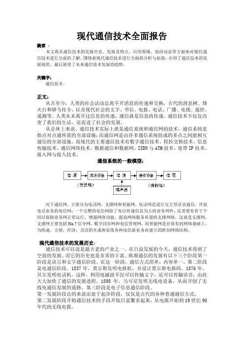
通信系统的一般模型：对于通信网，主要分为电话网，支撑网和智能网。

电话网是进行交互型话音通信，开放电话业务的电信网；一个完整的电信网除了有以传递信息为主的业务网外，还需要有若干个用以保障业务网正常运行，增强网络功能，提高网络服务质量的支撑网络，这就是支撑网，支撑网主要包括No.7信令网，数字同步网和电信管理网。

而智能网是在原有的网络基础上，为快速，方便，经济，灵活的生成和实现各种电信新业务而建立的附加网络结构。

现代通信技术的发展历史：通信技术可以说是最古老的产业之一。

在日益发展的今天，通信技术得到了空前的发展。

而它的历史也是非常的丰富。

纵观通信的发展有以下三个阶段第一阶段是语言和文字通信阶段。

在这一阶段，通信方式简单，内容单一。

第二阶段是电通信阶段。

1837年，莫尔斯发明电报机，并设计莫尔斯电报码。

1876年，贝尔发明电话机。

这样，利用电磁波不仅可以传输文字，还可以传输语音，由此大大加快了通信的发展进程。

1895年，马可尼发明无线电设备，从而开创了无线电通信发展的道路。

投资学课后答案APTChapter 10 Arbitrage Pricing Theory and Multifactor Models of Risk and Return Multiple Choice Questions1. ___________ a relationship between expected return and risk.A. APT stipulatesB. CAPM stipulatesC. Both CAPM and APT stipulateD. Neither CAPM nor APT stipulateE. No pricing model has found2. Consider the multifactor APT with two factors. Stock A has an expected return of 17.6%, a beta of 1.45 on factor 1 and a beta of .86 on factor 2. The risk premium on the factor 1 portfolio is3.2%. The risk-free rate of return is 5%. What is the risk-premium on factor 2 if no arbitrage opportunities exit?A. 9.26%B. 3%C. 4%D. 7.75%E. 9.75%3. In a multi-factor APT model, the coefficients on the macro factors are often called ______.A. systemic riskB. factor sensitivitiesC. idiosyncratic riskD. factor betasE. both factor sensitivities and factor betas4. In a multi-factor APT model, the coefficients on the macro factors are often called ______.A. systemic riskB. firm-specific riskC. idiosyncratic riskD. factor betasE. unique risk5. In a multi-factor APT model, the coefficients on the macro factors are often called ______.A. systemic riskB. firm-specific riskC. idiosyncratic riskD. factor loadingsE. unique risk6. Which pricing model provides no guidance concerning the determination of the risk premium on factor portfolios?A. The CAPMB. The multifactor APTC. Both the CAPM and the multifactor APTD. Neither the CAPM nor the multifactor APTE. No pricing model currently exists that provides guidance concerning the determination of the risk premium on any portfolio7. An arbitrage opportunity exists if an investor can construct a __________ investment portfolio that will yield a sure profit.A. small positiveB. small negativeC. zeroD. large positiveE. large negative8. The APT was developed in 1976 by ____________.A. LintnerB. Modigliani and MillerC. RossD. SharpeE. Fama9. A _________ portfolio is a well-diversified portfolio constructed to have a beta of 1 on one of the factors and a beta of 0 on any other factor.A. factorB. marketC. indexD. factor and marketE. factor, market, and index10. The exploitation of security mispricing in such a way that risk-free economic profits may be earned is called___________.A. arbitrageB. capital asset pricingC. factoringD. fundamental analysisE. technical analysis11. In developing the APT, Ross assumed that uncertainty in asset returns was a result ofA. a common macroeconomic factor.B. firm-specific factors.C. pricing error.D. neither common macroeconomic factors nor firm-specific factors.E. both common macroeconomic factors and firm-specific factors.12. The ____________ provides an unequivocal statement on the expected return-beta relationship for all assets, whereas the _____________ implies that this relationship holds for all but perhaps a small number of securities.A. APT; CAPMB. APT; OPMC. CAPM; APTD. CAPM; OPME. APT and OPM; CAPM13. Consider a single factor APT. Portfolio A has a beta of 1.0 and an expected return of 16%. Portfolio B has a beta of 0.8 and an expected return of 12%. The risk-free rate of return is 6%. If you wanted to take advantage of an arbitrage opportunity, you should take a short position in portfolio __________ and a long position in portfolio _______.A. A; AB. A; BC. B; AD. B; BE. A; the riskless asset14. Consider the single factor APT. Portfolio A has a beta of 0.2 and an expected return of 13%. Portfolio B has a beta of 0.4 and an expected return of 15%. The risk-free rate of return is 10%. If you wanted to take advantage of an arbitrage opportunity, you should take a short position in portfolio _________ and a long position in portfolio _________.A. A; AB. A; BC. B; AD. B; BE. No arbitrage opportunity exists.15. Consider the one-factor APT. The variance of returns on the factor portfolio is 6%. The beta of a well-diversified portfolio on the factor is 1.1. The variance of returns on thewell-diversified portfolio is approximately __________.A. 3.6%B. 6.0%C. 7.3%D. 10.1%E. 8.6%16. Consider the one-factor APT. The standard deviation of returns on a well-diversified portfolio is 18%. The standard deviation on the factor portfolio is 16%. The beta of thewell-diversified portfolio is approximately __________.A. 0.80B. 1.13C. 1.2517. Consider the single-factor APT. Stocks A and B have expected returns of 15% and 18%, respectively. The risk-free rate of return is 6%. Stock B has a beta of 1.0. If arbitrage opportunities are ruled out, stock A has a beta of __________.A. 0.67B. 1.00C. 1.30D. 1.69E. 0.7518. Consider the multifactor APT with two factors. Stock A has an expected return of 16.4%, a beta of 1.4 on factor 1 and a beta of .8 on factor 2. The risk premium on the factor 1 portfolio is 3%. The risk-free rate of return is 6%. What is the risk-premium on factor 2 if no arbitrage opportunities exit?A. 2%B. 3%C. 4%D. 7.75%E. 6.89%19. Consider the multifactor model APT with two factors. Portfolio A has a beta of 0.75 on factor 1 and a beta of 1.25 on factor 2. The risk premiums on the factor 1 and factor 2 portfolios are 1% and 7%, respectively. The risk-free rate of return is 7%. The expected return on portfolio A is __________ if no arbitrage opportunities exist.A. 13.5%B. 15.0%C. 16.5%D. 23.0%E. 18.7%20. Consider the multifactor APT with two factors. The risk premiums on the factor 1 and factor 2 portfolios are 5% and 6%, respectively. Stock A has a beta of 1.2 on factor 1, and a beta of 0.7 on factor 2. The expected return on stock A is 17%. If no arbitrage opportunities exist, the risk-free rate of return is ___________.A. 6.0%B. 6.5%C. 6.8%D. 7.4%E. 7.7%21. Consider a one-factor economy. Portfolio A has a beta of 1.0 on the factor and portfolio B has a beta of 2.0 on the factor. The expected returns on portfolios A and B are 11% and 17%, respectively. Assume that the risk-free rate is 6% and that arbitrage opportunities exist. Suppose you invested $100,000 in the risk-free asset, $100,000 in portfolio B, and sold short $200,000 of portfolio A. Your expected profit from this strategy would be ______________.A. ?$1,000B. $0C. $1,00022. Consider the one-factor APT. Assume that two portfolios, A and B, are well diversified. The betas of portfolios A and B are 1.0 and 1.5, respectively. The expected returns on portfolios A and B are 19% and 24%, respectively. Assuming no arbitrage opportunities exist, therisk-free rate of return must be ____________.A. 4.0%B. 9.0%C. 14.0%D. 16.5%E. 8.2%23. Consider the multifactor APT. The risk premiums on the factor 1 and factor 2 portfolios are 5% and 3%, respectively. The risk-free rate of return is 10%. Stock A has an expected return of 19% and a beta on factor 1 of 0.8. Stock A has a beta on factor 2 of ________.A. 1.33B. 1.50C. 1.67D. 2.00E. 1.7324. Consider the single factor APT. Portfolios A and B have expected returns of 14% and 18%, respectively. The risk-free rate of return is 7%. Portfolio A has a beta of 0.7. If arbitrage opportunities are ruled out, portfolio B must have a beta of__________.A. 0.45B. 1.00C. 1.10D. 1.22E. 1.33There are three stocks, A, B, and C. You can either invest in these stocks or short sell them. There are three possible states of nature for economic growth in the upcoming year; economic growth may be strong, moderate, or weak. The returns for the upcoming year on stocks A, B, and C for each of these states of nature are given below:25. If you invested in an equally weighted portfolio of stocks A and B, your portfolio return would be ___________ if economic growth were moderate.A. 3.0%D. 16.0%E. 17.0%26. If you invested in an equally weighted portfolio of stocks A and C, your portfolio return would be ____________ if economic growth was strong.A. 17.0%B. 22.5%C. 30.0%D. 30.5%E. 25.6%27. If you invested in an equally weighted portfolio of stocks B and C, your portfolio return would be _____________ if economic growth was weak.A. ?2.5%B. 0.5%C. 3.0%D. 11.0%E. 9.0%28. If you wanted to take advantage of a risk-free arbitrage opportunity, you should take a short position in _________ and a long position in an equally weighted portfolio of _______.A. A; B and CB. B; A and CC. C; A and BD. A and B; CE. No arbitrage opportunity exists.Consider the multifactor APT. There are two independent economic factors, F1and F2. The risk-free rate of return is 6%. The following information is available about two well-diversified portfolios:29. Assuming no arbitrage opportunities exist, the risk premium on the factor F1portfolio should be __________.A. 3%B. 4%C. 5%D. 6%E. 2%30. Assuming no arbitrage opportunities exist, the risk premium on the factor F2 portfolio should be ___________.A. 3%B. 4%C. 5%D. 6%E. 2%31. A zero-investment portfolio with a positive expected return arises when _________.A. an investor has downside risk onlyB. the law of prices is not violatedC. the opportunity set is not tangent to the capital allocation lineD. a risk-free arbitrage opportunity existsE. a risk-free arbitrage opportunity does not exist32. An investor will take as large a position as possible when an equilibrium price relationship is violated. This is an example of _________.A. a dominance argumentB. the mean-variance efficiency frontierC. a risk-free arbitrageD. the capital asset pricing modelE. the SML33. The APT differs from the CAPM because the APT _________.A. places more emphasis on market riskB. minimizes the importance of diversificationC. recognizes multiple unsystematic risk factorsD. recognizes multiple systematic risk factorsE. places more emphasis on systematic risk34. The feature of the APT that offers the greatest potential advantage over the CAPM is the ______________.A. use of several factors instead of a single market index to explain the risk-return relationshipB. identification of anticipated changes in production, inflation, and term structure as key factors in explaining the risk-return relationshipC. superior measurement of the risk-free rate of return over historical time periodsD. variability of coefficients of sensitivity to the APT factors for a given asset over timeE. superior measurement of the risk-free rate of return over historical time periods and variability of coefficients of sensitivity to the APT factors for a given asset over time35. In terms of the risk/return relationship in the APTA. only factor risk commands a risk premium in market equilibrium.B. only systematic risk is related to expected returns.C. only nonsystematic risk is related to expected returns.D. only factor risk commands a risk premium in market equilibrium and only systematic risk is related to expected returns.E. only factor risk commands a risk premium in market equilibrium and only nonsystematic risk is related to expected returns.36. The following factors might affect stock returns:A. the business cycle.B. interest rate fluctuations.C. inflation rates.D. the business cycle, interest rate fluctuations, and inflation rates.E. the relationship between past FRED spreads.37. Advantage(s) of the APT is(are)A. that the model provides specific guidance concerning the determination of the risk premiums on the factor portfolios.B. that the model does not require a specific benchmark market portfolio.C. that risk need not be considered.D. that the model provides specific guidance concerning the determination of the risk premiums on the factor portfolios and that the model does not require a specific benchmark market portfolio.E. that the model does not require a specific benchmark market portfolio and that risk need not be considered.38. Portfolio A has expected return of 10% and standard deviation of 19%. Portfolio B has expected return of 12% and standard deviation of 17%. Rational investors willA. borrow at the risk free rate and buy A.B. sell A short and buy B.C. sell B short and buy A.D. borrow at the risk free rate and buy B.E. lend at the risk free rate and buy B.39. An important difference between CAPM and APT isA. CAPM depends on risk-return dominance; APT depends on a no arbitrage condition.B. CAPM assumes many small changes are required to bring the market back to equilibrium; APT assumes a few large changes are required to bring the market back to equilibrium.C. implications for prices derived from CAPM arguments are stronger than prices derived from APT arguments.D. CAPM depends on risk-return dominance; APT depends on a no arbitrage condition, CAPM assumes many small changes are required to bring the market back to equilibrium; APT assumes a few large changes are required to bring the market back to equilibrium, implications for prices derived from CAPM arguments are stronger than prices derived from APT arguments.E. CAPM depends on risk-return dominance; APT depends on a no arbitrage condition and assumes many small changes are required to bring the market back to equilibrium.40. A professional who searches for mispriced securities in specific areas such as merger-target stocks, rather than one who seeks strict (risk-free) arbitrage opportunities is engaged inA. pure arbitrage.B. risk arbitrage.C. option arbitrage.D. equilibrium arbitrage.E. covered interest arbitrage.41. In the context of the Arbitrage Pricing Theory, as a well-diversified portfolio becomes larger its nonsystematic risk approachesA. one.B. infinity.C. zero.D. negative one.E. None of these is correct.42. A well-diversified portfolio is defined asA. one that is diversified over a large enough number of securities that the nonsystematic variance is essentially zero.B. one that contains securities from at least three different industry sectors.C. a portfolio whose factor beta equals 1.0.D. a portfolio that is equally weighted.E. a portfolio that is equally weighted and contains securities from at least three different industry sectors.43. The APT requires a benchmark portfolioA. that is equal to the true market portfolio.B. that contains all securities in proportion to their market values.C. that need not be well-diversified.D. that is well-diversified and lies on the SML.E. that is unobservable.44. Imposing the no-arbitrage condition on a single-factor security market implies which of the following statements?I) the expected return-beta relationship is maintained for all but a small number ofwell-diversified portfolios.II) the expected return-beta relationship is maintained for all well-diversified portfolios.III) the expected return-beta relationship is maintained for all but a small number of individual securities.IV) the expected return-beta relationship is maintained for all individual securities.A. I and III are correct.B. I and IV are correct.C. II and III are correct.D. II and IV are correct.E. Only I is correct.45. Consider a well-diversified portfolio, A, in a two-factor economy. The risk-free rate is 6%, the risk premium on the first factor portfolio is 4% and the risk premium on the second factor portfolio is 3%. If portfolio A has a beta of 1.2 on the first factor and .8 on the second factor, what is its expected return?A. 7.0%B. 8.0%C. 9.2%D. 13.0%E. 13.2%46. The term "arbitrage" refers toA. buying low and selling high.B. short selling high and buying low.C. earning risk-free economic profits.D. negotiating for favorable brokerage fees.E. hedging your portfolio through the use of options.47. To take advantage of an arbitrage opportunity, an investor wouldI) construct a zero investment portfolio that will yield a sure profit.II) construct a zero beta investment portfolio that will yield a sure profit.III) make simultaneous trades in two markets without any net investment.IV) short sell the asset in the low-priced market and buy it in the high-priced market.A. I and IVB. I and IIIC. II and IIID. I, III, and IVE. II, III, and IV48. The factor F in the APT model representsA. firm-specific risk.B. the sensitivity of the firm to that factor.C. a factor that affects all security returns.D. the deviation from its expected value of a factor that affects all security returns.E. a random amount of return attributable to firm events.49. In the APT model, what is the nonsystematic standard deviation of an equally-weighted portfolio that has an average value of σ(e i) equal to 25% and 50 securities?A. 12.5%B. 625%C. 0.5%D. 3.54%E. 14.59%50. In the APT model, what is the nonsystematic standard deviation of an equally-weighted portfolio that has an average value of σ(e i) equal to 20% and 20 securities?A. 12.5%B. 625%C. 4.47%D. 3.54%E. 14.59%51. In the APT model, what is the nonsystematic standard deviation of an equally-weighted portfolio that has an average value of σ(e i) equal to 20% and 40 securities?A. 12.5%B. 625%C. 0.5%D. 3.54%E. 3.16%52. In the APT model, what is the nonsystematic standard deviation of an equally-weighted portfolio that has an average value of σ(e i) equal to 18% and 250 securities?A. 1.14%B. 625%C. 0.5%D. 3.54%E. 3.16%53. Which of the following is true about the security market line (SML) derived from the APT?A. The SML has a downward slope.B. The SML for the APT shows expected return in relation to portfolio standard deviation.C. The SML for the APT has an intercept equal to the expected return on the market portfolio.D. The benchmark portfolio for the SML may be any well-diversified portfolio.E. The SML is not relevant for the APT.54. Which of the following is false about the security market line (SML) derived from the APT?A. The SML has a downward slope.B. The SML for the APT shows expected return in relation to portfolio standard deviation.C. The SML for the APT has an intercept equal to the expected return on the market portfolio.D. The benchmark portfolio for the SML may be any well-diversified portfolio.E. The SML has a downward slope, the SML for the APT shows expected return in relation to portfolio standard deviation, and the SML for the APT has an intercept equal to the expected return on the market portfolio are all false.55. If arbitrage opportunities are to be ruled out, each well-diversified portfolio's expected excess return must beA. inversely proportional to the risk-free rate.B. inversely proportional to its standard deviation.C. proportional to its weight in the market portfolio.D. proportional to its standard deviation.E. proportional to its beta coefficient.56. Suppose you are working with two factor portfolios, Portfolio 1 and Portfolio 2. The portfolios have expected returns of 15% and 6%, respectively. Based on this information, what would be the expected return on well-diversified portfolio A, if Ahas a beta of 0.80 on the first factor and 0.50 on the second factor? The risk-free rate is 3%.A. 15.2%B. 14.1%C. 13.3%D. 10.7%E. 8.4%57. Which of the following is (are) true regarding the APT?I) The Security Market Line does not apply to the APT.II) More than one factor can be important in determining returns.III) Almost all individual securities satisfy the APT relationship.IV) It doesn't rely on the market portfolio that contains all assets.A. II, III, and IVB. II and IVC. II and IIID. I, II, and IVE. I, II, III, and IV58. In a factor model, the return on a stock in a particular period will be related toA. factor risk.B. non-factor risk.C. standard deviation of returns.D. both factor risk and non-factor risk.E. There is no relationship between factor risk, risk premiums, and returns.59. Which of the following factors did Chen, Roll and Ross not include in their multifactor model?A. Change in industrial productionB. Change in expected inflationC. Change in unanticipated inflationD. Excess return of long-term government bonds over T-billsE. Neither the change in industrial production, change in expected inflation, change in unanticipated inflation, nor excess return of long-term government bonds over T-bills were included in their model.60. Which of the following factors did Chen, Roll and Ross include in their multifactor model?A. Change in industrial wasteB. Change in expected inflationC. Change in unanticipated inflationD. Change in expected inflation and Change in unanticipated inflationE. All of these factors were included in their model61. Which of the following factors were used by Fama and French in their multi-factor model?A. Return on the market index.B. Excess return of small stocks over large stocks.C. Excess return of high book-to-market stocks over low book-to-market stocks.D. All of these factors were included in their model.E. None of these factors were included in their model.62. Consider the single-factor APT. Stocks A and B have expected returns of 12% and 14%, respectively. The risk-free rate of return is 5%. Stock B has a beta of 1.2. If arbitrage opportunities are ruled out, stock A has a beta of __________.A. 0.67B. 0.93C. 1.30D. 1.69E. 1.2763. Consider the one-factor APT. The standard deviation of returns on a well-diversified portfolio is 19%. The standard deviation on the factor portfolio is 12%. The beta of thewell-diversified portfolio is approximately __________.A. 1.58B. 1.13C. 1.25D. 0.76E. 1.4264. Black argues that past risk premiums on firm-characteristic variables, such as those described by Fama and French, are problematic because ________.A. they may result from data snoopingB. they are sources of systematic riskC. they can be explained by security characteristic linesD. they are more appropriate for a single-factor modelE. they are macroeconomic factors65. Multifactor models seek to improve the performance of the single-index model byA. modeling the systematic component of firm returns in greater detail.B. incorporating firm-specific components into the pricing model.C. allowing for multiple economic factors to have differential effects.D. modeling the systematic component of firm returns in greater detail, incorporatingfirm-specific components into the pricing model, and allowing for multiple economic factors to have differential effects.E. none of these statements are true.66. Multifactor models such as the one constructed by Chen, Roll, and Ross, can better describe assets' returns byA. expanding beyond one factor to represent sources of systematic risk.B. using variables that are easier to forecast ex ante.C. calculating beta coefficients by an alternative method.D. using only stocks with relatively stable returns.E. ignoring firm-specific risk.67. Consider the multifactor model APT with three factors. Portfolio A has a beta of 0.8 on factor 1, a beta of 1.1 on factor 2, and a beta of 1.25 on factor 3. The risk premiums on the factor 1, factor 2, and factor 3 are 3%, 5% and 2%, respectively. The risk-free rate of return is 3%. The expected return on portfolio A is __________ if no arbitrage opportunities exist.A. 13.5%B. 13.4%C. 16.5%D. 23.0%E. 11.6%68. Consider the multifactor APT. The risk premiums on the factor 1 and factor 2 portfolios are 6% and 4%, respectively. The risk-free rate of return is 4%. Stock A has an expected return of 16% and a beta on factor 1 of 1.3. Stock A has a beta on factor 2 of ________.A. 1.33B. 1.05C. 1.67D. 2.00E. .95。

Diversity and Multiplexing:A Fundamental Tradeoff in Multiple-Antenna ChannelsLizhong Zheng,Member,IEEE,and David N.C.Tse,Member,IEEE Abstract—Multiple antennas can be used for increasing theamount of diversity or the number of degrees of freedom in wire-less communication systems.In this paper,we propose the pointof view that both types of gains can be simultaneously obtainedfor a given multiple-antenna channel,but there is a fundamentaltradeoff between how much of each any coding scheme canget.For the richly scattered Rayleigh-fading channel,we give asimple characterization of the optimal tradeoff curve and use it toevaluate the performance of existing multiple antenna schemes.Index Terms—Diversity,multiple input–multiple output(MIMO),multiple antennas,space–time codes,spatial multi-plexing.I.I NTRODUCTIONM ULTIPLE antennas are an important means to improvethe performance of wireless systems.It is widely under-stood that in a system with multiple transmit and receive an-tennas(multiple-input–multiple-output(MIMO)channel),thespectral efficiency is much higher than that of the conventionalsingle-antenna channels.Recent research on multiple-antennachannels,including the study of channel capacity[1],[2]andthe design of communication schemes[3]–[5],demonstrates agreat improvement of performance.Traditionally,multiple antennas have been used to increasediversity to combat channel fading.Each pair of transmit andreceive antennas provides a signal path from the transmitter tothe receiver.By sending signals that carry the same informationthrough different paths,multiple independently faded replicasof the data symbol can be obtained at the receiver end;hence,more reliable reception is achieved.For example,in a slowRayleigh-fading environment with one transmit and receiveantennas,the transmitted signal is passed throughcan beachieved:the average error probability can be made to decaylikeof each type of gain any coding scheme can extract:higher spatial multiplexing gain comes at the price of sacrificing diversity.Our main result is a simple characterization of the optimal tradeoff curve achievable by any scheme.To be more specific,we focus on the high-SNR regime,and think of a scheme as a family of codes,one for each SNR level.A scheme is said to have a spatial multiplexinggainif the rate of the scheme scalesliketheoptimal diversityadvantageprovided by the channel;andsymbols.We show that as long as the blocklength,the optimal diversitygain(transmitandreceive antennas were used for multiplexing and theremainingas longas ;hence,no more diversity gain can be extracted by coding over block lengths greaterthanthan using a block length equalto .The tradeoff curve can be used as a unified framework to com-pare the performance of many existing diversity-based and mul-tiplexing-based schemes.For several well-known schemes,wecompute the achieved tradeoffcurvesand compare it to the optimal tradeoff curve.That is,the performance of a scheme is evaluated by the tradeoff it achieves.By doing this,we take into consideration not only the capability of the scheme to combat against fading,but also its ability to accommodate higher data rate as SNR increases,and therefore provide a more complete view.The diversity–multiplexing tradeoff is essentially the tradeoff between the error probability and the data rate of a system.A common way to study this tradeoff is to compute the relia-bility function from the theory of error exponents [10].How-ever,there is a basic difference between the two formulations:while the traditional reliability function approach focuses on the asymptotics of large block lengths,our formulation is based on the asymptotics of high SNR (but fixed block length).Thus,in-stead of using the machinery of the error exponent theory,we exploit the special properties of fading channels and develop a simple approach,based on the outage capacity formulation [11],to analyze the diversity–multiplexing tradeoff in the high-SNR regime.On the other hand,even though the asymptotic regimeis different,we do conjecture an intimate connection between our results and the theory of error exponents.The rest of the paper is outlined as follows.Section II presents the system model and the precise problem formulation.The main result on the optimal diversity–multiplexing tradeoff curve is given in Section III,for blocklength .In Sec-tion IV ,we derive bounds on the tradeoff curve when the blocklength is lessthan.While the analysis in this sec-tion is more technical in nature,it provides more insights to the problem.Section V studies the case when spatial diversity is combined with other forms of diversity.Section VI discusses the connection between our results and the theory of error ex-ponents.We compare the performance of several schemes with the optimal tradeoff curve in Section VII.Section VIII contains the conclusions.II.S YSTEM M ODEL AND P ROBLEM F ORMULATIONA.Channel ModelWe consider a wireless linkwithis the complex path gainfrom transmitantennabeing the signals transmitted from antenna;attimesymbol times.In Section V ,our results are generalizedto the case when there is a multiple of such blocks,each of which experiences independent fading.AratecodewordsZHENG AND TSE:FUNDAMENTAL TRADEOFF IN MULTIPLE-ANTENNA CHANNELS 1075B.Diversity and MultiplexingMultiple-antenna channels provide spatial diversity ,which can be used to improve the reliability of the link.The basic idea is to supply to the receiver multiple independently faded replicas of the same information symbol,so that the probability that all the signal components fade simultaneously is reduced.As an example,consider uncoded binary phase-shift keying (PSK)signals over a single-antenna fading channel(in the above model).It is well known [12]that the proba-bility of error at high SNR (averaged over the fadinggain as well as the additive noise)isHere,we observe that by having the extra receive antenna,the error probability decreases with SNR at a faster speedof.Similar results can be obtained if we change the binary PSK signals to other constellations.Since the performance gain at high SNR is dictated by the SNR exponent of the error prob-ability,this exponent is called the diversity gain .Intuitively,it corresponds to the number of independently faded paths that a symbol passes through;in other words,the number of indepen-dent fading coefficients that can be averaged over to detect the symbol.In a general systemwithwhere(b/s/Hz),in contrasttofor single-antenna channels.This result suggests thatthe multiple-antenna channel can be viewedas parallel spatial channels ;hence thenumber is the total number of degrees of freedom to communicate.Now one can transmit independent information symbols in parallel through the spatial channels.This idea is also called spatial multiplexing .Reliable communication at rates arbitrarily close to the er-godic capacity requires averaging across many independent re-alizations of the channel gains over time.Since we are consid-ering coding over only a single block,we must lower the data rate and step back from the ergodic capacity to cater for the ran-domness of thechannel .Since the channel capacity increaseslinearlywith,in order to achieve a certain fraction of the capacity at high SNR,we should consider schemes that sup-port a data rate which also increases with SNR.Here,we thinkof a scheme as a family ofcodesof blocklength(b/s/Hz)and diversitygain(3)Foreachare similarly defined.Equation (3)can,thus,bewrittenas1076IEEE TRANSACTIONS ON INFORMATION THEORY,VOL.49,NO.5,MAY2003 commonly used as a diversity criterion in space–time codedesign.•In the standard formulation,diversity gain is an asymptoticperformance metric of one fixed code.To be specific,theinput of the fading channel is fixed to be a particular code,while SNR increases.The speed that the error probability(of a maximum-likelohood(ML)detector)decays as SNRincreases is called the diversity gain.In our formulation,we notice that the channel capacity increases linearlywith.Hence,in order to achieve a nontrivial fraction of the capacity at high SNR,the input data rate must also in-crease with SNR,which requires a sequence of codebooks with increasing size.The diversity gain here is used as a performance metric of such a sequence of codes,which is formulated as a“scheme.”Under this formulation,any fixed codehasmeasures how far the SNR is above theminimal required to support the target data rate.A dual way to characterize the performance is to plot the errorprobability as a function of the data rate,for a fixed SNR level.Analogous to Forney’s formulation,to take into considerationthe effect of the SNR,one should use the normalized datarate;hence,thespatial multiplexinggainis just a constant multipleofC ASEIn this section,we will derive the optimal tradeoff between thediversity gain and the spatial multiplexing gain that any schemecan achieve in the Rayleigh-fading multiple-antenna channel.We will first focus on the case that the blocklength,and discuss the other cases in Section IV.Fig.1.Diversity–multiplexing tradeoff,dm l r drrnnme n ma m m l l mu l l nnmam l di rnndn n ne l n n mo r de r r d m;ZHENG AND TSE:FUNDAMENTAL TRADEOFF IN MULTIPLE-ANTENNA CHANNELS1077Fig. 2.Adding one transmit and one receive antenna increases spatial multiplexing gain by 1at each diversity level.correspondsto .Theorem 2makes a more informative statement:if we increaseboth,as shownin Fig.2;i.e.,for any given diversity gainrequirement.The optimal tradeoff for this channelis plotted in Fig.3(a).The maximum diversity gain for thischannelis,and the total number of degrees of freedom in the channelis.Ifwe increase the size of the constellation for thesymboland the max-imal diversity provided by thechannel .For the precedingexample,in theform,since onesymbol is transmitted per symbol time.This is twice as much as that for the repetition scheme.However,the tradeoff curve achieved by the Alamouti scheme is still below the optimal for any1078IEEE TRANSACTIONS ON INFORMATION THEORY ,VOL.49,NO.5,MAY 2003In the literature on space–time codes,the diversity gain of a scheme is usually discussed for a fixed data rate,correspondingto a multiplexinggain .This is,in fact,the maximal diver-sitygain,one cannot distinguish the performance ofthe repetition scheme in (5)and the Alamouti scheme.More generally,the problem of finding a code with the highest (fixed)rate that achieves a given diversity gain is not a well-posed one:any code satisfying a mild nondegenerate condition (essentially,a full-rank condition like the one in [7])will have full diver-sity gain,no matter how dense the symbol constellation is.This is because diversity gain is an asymptotic concept,while for any fixed code,the minimum distance is fixed and does not de-pend on the SNR.(Of course,the higher the rate,the higher the SNR needs to be for the asymptotics to be meaningful.)Inthe space–time coding literature,a common way to get around this problem is to put further constraints on the class of codes.In [7],for example,each codewordsymbolis constrained to come from the same fixed constellation (c.f.[7,Theorem 3.31]).These constraints are,however,not fundamental.In contrast,by defining the multiplexing gain as the data rate normalized by the capacity,the question of finding schemes that achieves the maximal multiplexing gain for a given diversity gain becomes meaningful.B.Outage FormulationAs a step to prove Theorem 2,we will first discuss another commonly used concept for multiple-antenna channels:the outage capacity formulation,proposed in [11]for fading channels and applied to multiantenna channels in [1].Channel outage is usually discussed for nonergodic fadingchannels,i.e.,the channelmatrixis chosen randomly but is held fixed for all time.This nonergodic channel can be writtenas(7)where,andand the channel realization.Without loss of optimality,the input distribution can be taken to be Gaussian with a covari-ancematrixto get an upper bound on theoutage probability.On the otherhand,is a positive-semidefinite matrix.Noticethatis an increasing function on the cone of positive-definite Hermitian matrices,i.e.,ifby hence,the outage probabilitysatisfies (9)and we can without loss of generality assume the input (Gauss-ian)distribution to have covariancematrixwhich scaleswithaswhereZHENG AND TSE:FUNDAMENTAL TRADEOFF IN MULTIPLE-ANTENNA CHANNELS1079ratetofor;hence,.Wecan also generalize to the case that the fading distributionhas.In ageneral,with aprobability.To generalize this idea tomultiple-antenna systems,we need to study the probability thatthe singular valuesof are close to zero.We quote the jointprobability density function(pdf)of these singular values[14].Lemma3:Let bean.The precedingexpression can thus be writtenasindicates the level of singularityof the channelmatrix.Thelargerdescribes the outageevent in terms of the singularity level.With the distributionof,i.e.,with is the setofreal,and thus has no effect on the SNR exponent,andforany1080IEEE TRANSACTIONS ON INFORMATION THEORY,VOL.49,NO.5,MAY2003 Theorem4(Outage Probability):For the multiple-antennachannel(1),let the data ratebe,with.The outage probabilitysatisfies(13)wherecan be explicitly computed.Theresulting.Proof:See theAppendix.(15)which characterizes the near-singular distribution of the channelmatrix.This result has a geometric interpretation as follows.For,defineis a differentiable manifold;hence,the dimensionalityof,one needs tospecifyrows as a linear combination of them.These addupto,is the boundaryofinis near singular if it is close to theboundary,occurswhen is close to itsprojection,.This means that the componentofin dimensions is oforder.Conditioned on this event,the secondsmallest singular valueof beingsmall,is close to its boundary,with aprobability.By induction,(15)is obtained.Now the outage event at multiplexinggain.There are many choicesofthat leadto outage,one particularchoicetakes an integervalueforsmallest singularvalueslargest singular values are oforderis not an integer,say,andbetween integers,only one singular value of,corresponding to the typicalZHENG AND TSE:FUNDAMENTAL TRADEOFF IN MULTIPLE-ANTENNA CHANNELS1081 outage event,is adjusted to be barely large enough to supportthe data rate;therefore,the SNR exponent of the outageprobability,(16)whereofsize.Since the channel fading coefficientsin are notknown at the transmitter,we can assumethat is independentof.Conditioned on a specific channelrealization,writethe mutual information of the channelaserrorasin thesetNow choose theinput tominimize,we haveThis result says that conditioned on the channel outageevent,it is very likely that a detection error occurs;therefore,the outage probability is a lower bound on the error probability.The outage formulation captures the performance under infi-nite coding block length,since by coding over an infinitely longblock,the input can be reliably detected as long as the data rateis below the mutual information provided by the random real-ization of the channel.Intuitively,the performance improves asthe block length increases;therefore,it is not too surprising thatthe outage probability is a lower bound on the error probabilitywith any finite blocklength,Theorem2,however,contains a stronger result:with a finite blocklength,this bound is tight.That is,no more diversity gaincan be obtained by coding over a block longerthan,since the infinite block length performance is already achieved.Consider now the use of a random code for the multiantennafading channel.A detection error can occur as a result of thecombination of the following three events:the channelmatrixis atypically ill-conditioned,the additive noise is atypicallylarge,or some codewords are atypically close together.By goingto the outage formulation(effectively taking,the randomness in the last twoevents is averaged out.Consequently,when there is no outage,the error probability is very small;the detection error is mainlycaused by the bad channel event.With a finite blocklength,given thatthere is no channel outage,the error probability(for an i.i.d.Gaussian input)has an SNR exponent that is not smaller thanthat of the outage probability;hence,outage is still the domi-nating error event,as intheare two possible transmitted codewords,and.Suppose,conditioned on a certain realization of thechannel,is1082IEEE TRANSACTIONS ON INFORMATION THEORY ,VOL.49,NO.5,MAY 2003where is the additive noise on the directionofonly through the singular values.Letfor,wehave(19)A v e r a g i n g w i t h r e s p e c t t o t h e d i s t r i b u t i o n of,theminimum always occurswith,An alternative derivation of the bound (18)on the PEP gives some insight to the typical way in which pairwise error occurs.Letbe the nonzero eigenvaluesof .Sincedenotes equality in distribution.ConsiderThis probability is boundedby,from(15)Combining these,wehave,i.e.,it has the same order of magnitude as theadditive noise.D.Relationship to the Naive Union BoundThe key idea of the proof of Theorem2is to find the rightway to apply the union bound to obtain a tight upper boundon the error probability.A more naive approach is to directlyapply the union bound based on the PEP.However,the followingargument shows that this union bound is not tight.Consider the case when the i.i.d.Gaussian random code isused.It follows from(21)that the average PEP can be approx-imatedasis the difference between codewords.Denote.Giventhatoccurs,the channel is in deep fade and itis very likely that a detection error occurs.The average PEP is,therefore,lower-boundedby:,is plotted in Fig.4,in comparison to the optimaltradeoffcurve,even when we applied(22)to have an“optimistic”bound,it is still below theoptimalFig.4.Union bound of PEP.tradeoff curve.Therefore,we conclude that the union bound onthe average PEP is a loose bound on the actual error probability.This strongly suggests that to get significant multiplexing gain,a code design criterion based on PEP is not adequate.The reason that this union bound is not tight is as follows.Suppose is the transmitted codeword.When the channelmatrix isill-conditioned,is closeto formanyand then bound the error probability conditioned on the channelhaving no outage with the union bound based on the conditionalPEP.By doing this,we avoid the overcounting in the unionbound,and get a tight upper bound of the error probability.Itturns out thatwhen,the second term of thepreceding inequality has the same SNR exponent as the outageprobability,which leads to the matching upper and lower boundson the diversitygainissmall,with a random code from the i.i.d.Gaussian ensemble,the probability that some codewords are atypically close to eachother becomes significant,and the outage event is no longer thedominating error event.In this section,we will develop differenttechniques to obtain tighter bounds,which also provide more in-sights into the error mechanism of the multiple-antenna channel.A.Gaussian Coding BoundIn the proof of Theorem2,we have developed an upper boundon the error probability,which,in fact,applies for systems withany valuesofwhere the minimization is taken over thesetcan be computed explicitly.For conve-nience,we call a systemwithsystem,and define the func-tion,also writtenasis a linear function with theslope.For,has slope,which is strictlybelowand areplotted in Fig.5,with and2,respectively.In the next subsection,we will explore how the Gaussiancoding bound can beimproved.Fig.5.Upper and lower bounds for the optimal tradeoff curve.B.Typical Error EventThe key idea in the proof of Theorem2is to isolate a“bad-channel”event(26)and compute the error probability in the second term with theunion bound valuesof,it is loosefor.A natural attempt to improvethis bound is to optimize over the choicesofbe the nonzero eigenvaluesofasTo find the optimal choiceofforall;hence,furtherboundingby,the right-hand sideof(28)is lessthantoobtain the tightest upper bound from(26)is simply the outageevent.Discussion—Typical Error Event:Isolating the outage eventessentially bounds the conditional error probabilityby.For convenience,weassumealwayssatisfies,a detection error typ-ically occurswhen;in otherwords,when the channel has a singularity levelof,wehave,which is the same singularity level of the typical outage event;therefore,the detection error is typically caused by the channeloutage.On the other hand,when,we have forsome,correspondingtoofsize generated from the i.i.d.Gaussian ensemble.Fix a channelrealization.Assumethat is the transmitted codeword.For any othercodewordLet be the ordered nonzero eigen-valuesof.Writeis isotropic,it has the samedistributionas.Following(21),the PEP can beapproximatedas,with,anerror occurswhenwith a probability oforder,forall,wehavec o n t a i n i n g c ode w o r d s,w i t h p r o b-a b i l i tyt h a t a r e a t y p i c a l l y c l o s e t o.S u c h a“b a d c o d e w o r d”o c c u r s r a r e l y(w i t h p r o b a b i l i t y),b u t h a s a l a r g e p r o b-a b i l i t y t o b e c o n f u s e d w i t h t h e t r a n s m i t t e d c o d e w o r d;h e n c e,t h i s e v e n t d o m i n a t e s t h e o v e r a l l e r r o r p r o b a b i l i t y o f t h e c o d e.T h i s r e s u l t s u g g e s t s t h a t p e r f o r m a n c e c a n b e i m p r o v e d b yex-purgating these bad codewords.C.Expurgated BoundThe expurgation of the bad codewords can be explicitly car-ried out by the following procedure:3•Step1Generate a random codebook ofsize,witheachcodeword.Bychoosingk(30)for small .In fact,this property holds for any other distributions,from which thecodewords are independently generated.To see this,assume r2C0r(0)=.A l s o,(30)i s c e r t a i n l y t r u e f o r t h e d i s t r i b u t i o n s w i t h p r o b a b i l i t y m a s s e s ord e f i n e d i n(25).T h i s t h e o r e m g i v e s t h e f o l l o w i n g i n t e r e s t i n gb e t w e e n t h e G a u s s i a nc od i n g b o u n d de r i v e d i n Lt h e e x p u r g a t e d b o u n d:f o r a ns y s t e m w i t ho n e c a n g e t,f r o m i s o l a t i ng th e o u t a g e e v e n t,a di v e r s i t y g at r a n s m i t,a t a s p a t i a l m u l t i p l e x i n g g a i n o f,o n e c a n g e t a d i v e r s i t y g a i n ofa n d c o m p u t e t h e u p p e rb o u n d o n t h e e r r o r pr.S i n cea p p r o a c h e se r r or,a d i v e r s i t ys u c h t h a t b o t h t e r m s i n(31)a r e u p p e r-b o u n d e d b y,i.e.,t ob e e x p u r g a t e d t o i m p r o v e t h e e r r o r p r o b a b i l i t y o fc ode b o o k.C l e a r l y,t h e m o r e w e e x p u r g a t e,t h ep r o b a b i l i t y w e c a n g e t.H o w e v e r,t o m a k e s u r e te n o u g h c o d e w o r d s l ef t t o c a r r y t h e d e s i r e d d a t arNow with the expurgated codebook,the error probability(from union bound and(21))isare i.i.d.Gaussian distributed.If weexchangeand,,,andforand.,correspondingto the pointswith,which again matcheswith the upperbound.In this case,the maximal diversitygain.To see this,consider binary detectionwithand being the two possible codewords.Let.We candecompose the row vectorsof into the componentsindimensions,and.If,which has a proba-bility of orderwhenandcan achieve adiversitygain.First we can construct anotherschemeto be the transmitted code-word,lettransmitted-dimensional componentofin the directionofis trans-mitted is strictly largerthan.Since the average error probabilityis,there must be a majority of codewords,say,half of them,for which the nearest neighbor is atleastis not changed.Thisschemecodewords.Consequently,all theother .In this section,we consider the casewhen one can codeoverBlocks):For the block-fadingchannel,with a scheme that codesoverb/block),the optimal errorprobability is upper-boundedbyforforblocks.Hence,if we can afford to increase the codelengthin each channel use,and trade that for a higher data rate.Compare to the case when coding over single block,since both the upper and lower bounds on the SNR exponent are mul-tiplied by the samefactor;andfor.This corollary can be proved by directly applying the tech-niques we developed in the previous sections.Intuitively,with a code oflength.As an example,we consider the PEP.In contrast to(21),with codingoverforblocks.VI.C ONNECTION TO E RROR E XPONENTSThe diversity–multiplexing tradeoff is essentially the tradeoff between the error probability and the data rate of a communica-tion system.A commonly used approach to study this tradeoff for memoryless channels is through the theory of error expo-nents [10].In this section,we will discuss the relation between our results and the theory of error exponents.For convenience,we quote some results from [10].Lemma 9(Error Exponents):For a memoryless channel with transition probabilitydensityandrate(37)whereas,andsatisfying the input constraint,and(actually,we con-sideredterms have to be computed as well.Thus,while the theory of error ex-ponents is catered for characterizing the error probability for large blocklength.While we have not been able to verify this conjecture,we have shown that if we fix the inputdistributionandratesatisfying the input constraint,and(38)for-by-,and compare itagainst the optimal tradeoffcurve。