Finite element modelling of deformation characteristics of historical stone masonry shear walls
- 格式:pdf
- 大小:16.80 MB
- 文档页数:14
the mathematical theory of finiteelement methodThe mathematical theory of the finite element method (FEM) is a branch of numerical analysis that provides a framework for approximating solutions to partial differential equations (PDEs) using discretization techniques. The finite element method is widely used in engineering and scientific disciplines to simulate and analyze physical phenomena.At the core of the FEM is the concept of dividing a domain into a finite number of elements, which are connected at nodes. The unknown solution within each element is approximated using a simple function, referred to as the basis function. These basis functions are usually polynomials of a certain degree, and their coefficients are determined by solving a set of linear equations.The mathematical theory of the FEM involves several key concepts and techniques. One of the fundamental principles is the variational formulation, which transforms the PDE into an equivalent variational problem. This variational problem is then discretized using the finite element approximation, resulting in a system of algebraic equations.Another important aspect is the assembly process, where the contributions from each element are combined to form the global stiffness matrix and right-hand side vector. This assembly is based on the integration of the basis functions and their derivatives over the element domains.Error estimation and convergence analysis are also essential components of the mathematical theory of the FEM. Various techniques, such as the energy method and the posteriori error estimators, are used to assess the accuracy of the finite element solution and to determine the appropriate mesh refinement for achieving convergence.Furthermore, the mathematical theory of the FEM includes the treatment ofboundary conditions, imposition of symmetries, and the development of efficient solvers for the resulting linear systems. It also addresses issues such as numerical stability,并行 computing, and adaptivity.In summary, the mathematical theory of the finite element method provides a comprehensive framework for numerically solving PDEs. It encompasses concepts such as element discretization, variational formulation, assembly, error estimation, and convergence analysis, which collectively enable the accurate and efficient simulation of a wide range of physical problems.。
轧制过程中粗轧宽度变形的三维有限元模拟杨正波(梅山钢铁公司技术中心 南京 210039) 摘 要:应用MARC/autoforge商用有限元软件,对长方形轧件在热轧粗轧过程的宽度变形过程进行热力耦合模拟。
简介了宽展的种类及其组成,模拟研究中主要计算了板坯在粗轧过程中的宽展量。
分析计算说明,采用有限元模拟的方法可以较好地反映板坯宽度变形的实际情况。
关键词:宽度变形;轧制;有限元模拟Simulation of Three Dimensional Finite Element of WidthDeformation for Rougher in the Rolling ProcessYang Zhengbo(Technology Center of Meishan Iron&Steel Co.,Nanjing210039) K ey w ords:Widt h deformation;Rolling;Finite element simulation0 引 言 根据给定的坯料尺寸和压下量,来确定轧制后产品的尺寸,或者已知轧制后轧件的尺寸和压下量,要求定出所需坯料的尺寸,这是在拟订轧制工艺时首先遇到的问题。
要解决这类问题,首先要解决被压下金属的体积是如何沿轧制方向和宽度方向分配的,亦即如何分配延伸和宽展的。
因为只有知道了延伸及宽展的大小后,按照体积不变条件才有可能在已知轧前坯料尺寸及压下量的前提下,计算轧制后产品的尺寸;或者根据轧制后轧件的尺寸来推算轧制前所需要的坯料尺寸。
由此可见,研究轧制过程中宽展的规律具有很大实际意义。
1 宽展的种类和组成1.1 宽展的种类 在不同的轧制条件下,坯料在轧制过程中的宽展形式是不同的。
根据金属沿横向上流动的自由程度,宽展可分为自由宽展、限制宽展和强制宽展3种。
(1)自由宽展 坯料在轧制过程中,被压下的金属体积可以自由展宽的量。
此时,金属的流动除来自轧辊的摩擦阻力外,不受任何限制。
FINITE ELEMENT MODEL DEVELOPMENT AND VALIDATION FOR AIRCRAFT FUSELAGE STRUCTURESRalph D. Buehrle, Gary A. Fleming and Richard S. PappaNASA Langley Research CenterandFerdinand W. GrosveldLockheed Martin Engineering and Sciences18th International Modal Analysis ConferenceSan Antonio, TexasFebruary 7-10, 2000FINITE ELEMENT MODEL DEVELOPMENT AND VALIDATION FOR AIRCRAFT FUSELAGE STRUCTURESRalph D. Buehrle, Gary A. Fleming and Richard S. PappaNASA Langley Research CenterandFerdinand W. GrosveldLockheed Martin Engineering and SciencesAbstractThe ability to extend the valid frequency range for finite element based structural dynamic predictions using detailed models of the structural components and attachment interfaces is examined for several stiffened aircraft fuselage structures. This extended dynamic prediction capability is needed for the integration of mid-frequency noise control technology. Beam, plate and solid element models of the stiffener components are evaluated. Attachment models between the stiffener and panel skin range from a line along the rivets of the physical structure to a constraint over the entire contact surface. The finite element models are validated using experimental modal analysis results. The increased frequency range results in a corresponding increase in the number of modes, modal density and spatial resolution requirements. In this study, conventional modal tests using accelerometers are complemented with Scanning Laser Doppler Velocimetry and Electro-Optic Holography measurements to further resolve the spatial response characteristics. Whenever possible, component and subassembly modal tests are used to validate the finite element models at lower levels of assembly. Normal mode predictions for different finite element representations of components and assemblies are compared with experimental results to assess the most accurate techniques for modeling aircraft fuselage type structures. NomenclatureATC Aluminum Testbed CylinderEOH Electro-Optic HolographyERA Eigensystem Realization AlgorithmDOF(s)degree(s) of freedomFE finite elementFRF(s)frequency response function(s)Hz HertzMIF(s)mode indicator function(s)psig pounds per square inch gaugeSLDV Scanning Laser Doppler VelocimetryIntroductionImproved mid-frequency structural vibration and acoustic response predictions are required for design optimization and noise control applications in the aerospace and transportation industries. Finite element (FE) and boundary element methods are generally used for low frequency predictions where discrete modal behaviors dominate. Statistical energy analysis [1] and energy finite element analysis [2] are used in the high frequency region, characterized by high modal density. In the mid-frequency region, the assumption of high modal density used in the energy analysis formulations is no longer valid. Finite element analysis in the mid-frequency region becomes more difficult because the structural vibration wavelength decreases with increasing frequency requiring a finer element mesh to describe the dynamic response. Advances in computer technology provide the capability to solve FE analyses of increasing complexity. In this paper, the ability to extend the valid frequency range for FE based structural dynamic predictions using detailed models of the components and attachment interfaces is examined. Normal mode predictions for different finite element representations of components and assemblies are compared with experimental results to assess the most accurate techniques for modeling aircraft fuselage type structures.Hardware DescriptionThis paper focuses on two stiffened aircraft fuselage structures. The first structure is the Aluminum Testbed Cylinder (ATC). Figures 1 and 2 show the primary components of the ATC. The cylindrical section of the ATC is an all-aluminum structure that is 12 feet in length and 4 feet in diameter. The shell consists of a 0.040-inch thick skin that is stiffened by 11 ring frames and 24 equally spaced longitudinal stringers. Double lines of rivets and epoxy are used to attach the skin to the frames and stringers. The floor is constructed of aluminum honeycomb and is supported by cross members at each of the ring frames. Two-inch thick particleboard end plates provide stiff, terminating reflective surfaces for the enclosed acoustic cavity. The end plates contain several ½-inch diameter holes to allow the pressure on each side of the end plates to equalize during pressurized tests. The end domes are ¼-inch thick fiberglass composite structures allowing for pressurization of the interior to 7 psig to simulate flight conditions at altitudes up to 35000 feet. The second structure is an aluminum fuselage panel shown in Figure 3. The panel is representative of current aircraft construction but was manufactured without curvature to simplify the experimental and analytical modeling. The 47-by 72-inch aluminum panel consists of a 0.050-inch skin with six equally spaced longitudinal stringers and four equally spaced frame stiffeners. Single lines of rivets attach the stringers and frames to the skin. As shown in Figure 3, a bay is defined as a section of the panel skin that is bounded by the stringers and frames. The bay responses are the focus of the fuselage panel correlation efforts.Numerical ModelingGeometric and finite element models of the fuselage structures were developed in MSC/PATRAN. The models were generated based on the physical dimensions and material properties of the structures as specified in the manufacturing drawings. Normal mode analysis of the FE models was performed using the Lanczos method in MSC/NASTRAN.A detailed description of the baseline ATC finite element model is provided by Grosveld [3]. FE models of an isolated ring frame and longitudinal stringer were developed using bar, beam, plate, and solid elements. In addition, a hybrid model combining beam and plate elements was used to provide the required load path near the cutouts in the ring frame while attempting to minimize the number of degrees of freedom (DOFs). Normal mode predictions for the component models are compared with modal test data to assess the required level of modeling detail.The ATC framework, consisting of the interconnected ring frames and longitudinal stringers, was modeled using linear plate elements. Coincident nodes at the frame to stringer intersections were equivalenced. This constrains all six DOFs between the frames and stringers at these nodes. One motivation for using the 2-dimensional plate element for the frames and stringers is for the attachment of the skin. As described previously, the skin of the cylinder is attached to the frames and stringers using a double line of rivets and epoxy. The additional dimension provided by the plate elements allows the skin to be constrained over the width of the stiffener. In this way, each bay (unsupported skin section bounded by the frames and stringers) has the correct dimensions. A model of the baseline ATC including the cylinder frame with the skin attached was developed using linear plate elements. The coincident nodes at the stiffener to skin attachment locations were equivalenced. Normal mode predictions for the frame and baseline cylinder will be compared with modal test data.Finite element modeling of the fuselage panel [4] has focused on different stiffener to skin attachment models and their effects on the predicted bay motions. To characterize the panel dynamic response up to 1000 Hz, several methods of modeling the panel were examined. First, the required finite element mesh density of the panel skin was evaluated by performing a normal mode analysis of a single bay with clamped boundary conditions. The skin was modeled with linear plate elements. A mesh of 30 by 16 elements was found to provide a one-percent convergence on frequency and adequate spatial resolution to define the mode shapes through 1000 Hz. This resulted in 11682 linear plate elements for the overall panel skin.After establishing the model for the panel skin, three methods of modeling the stiffeners were evaluated. The simplest method is to model the stiffeners with beam elements. The beam elements are one-dimensional elements that have the effective cross-sectional properties (area, inertia’s, and torsional constant) of the stiffeners. Offsets from the skin to the stiffener neutral axis are also included. The beam elements are created along a line consistent with the rivet line that attaches the skin to the stiffeners. The beam stiffener model of the panel contains approximately 60,000 DOFs.A second method of modeling the stiffeners is to use two-dimensional linear plate elements. This requires a detailed model of the geometry of the stiffeners. The plate element model of the stiffeners can then be attached to the skin elements over the entire contact surface or along a line consistent with the rivet line on the physical structure. Normal mode analyses were performed for both the surface and rivet line constraint. The plate stiffener model with rivet line attachment contains approximately 141,000 DOFs.A third hybrid model of the stiffeners was generated to minimize the DOFs and provide the required load path near sections with cutouts. The frame sections with cutouts were modeled with plate elements and the stringers with continuous cross-sections were modeled with beam elements. For this model, the stiffener to skin attachment was along the rivet line. The hybrid stiffener model of the fuselage panel contains approximately 71,000 DOFs. Experimental ValidationExperimental modal analysis results were used to validate the normal mode predictions of the various finite element models. Modal tests of an isolated ring frame and longitudinal stringer were performed to verify the ATC component models. These tests were conducted with the structures suspended from bungee chord to simulate free-free conditions. Frequency response functions (FRFs) were acquired between the four reference accelerometers and impact force. Sufficient impact positions were used to capture the modal properties over the 0 to 200 Hz frequency range. The polyreference curevefitter in the Spectral Dynamics STAR software was used to determine the modal properties from the FRF data.To facilitate model updating, modal tests are planned for seven different levels of assembly for the ATC. Three assembly level modal tests have been conducted on the ATC [5]. First, the cylinder framework, composed of the interconnected ring frames and stringers, was tested prior to application of the skin. The second test configuration added the end plates to the cylinder frame. The third configuration is the baseline cylinder shown in figure 4, which is composed of the cylinder framework from configuration 1 with the skin applied. In each test configuration, the structure was supported by bungee chord to simulate free-free boundary conditions. The assembly level tests were conducted with multi-point random excitation and 207 accelerometer response measurements. The excitation and response measurement positions were selected based on pre-test predictions of the first 100 modes. FRFs were acquired over the 0 to 1000 Hz bandwidth. Because of the large number of modes excited in each test and the relatively low damping levels, Fourier transform block sizes as high as 64K were used. Mode indicator functions (MIFs) [6] were calculated from the FRFs to provide an estimate of the natural vibration frequencies of the structure. The Eigensystem Realization Algorithm (ERA) [7] was used to identify the modal parameters (natural frequencies, damping factors, and mode shapes) for each test configuration. Future tests of the ATC will incorporate the end plates, the domes, and the floor(configurations 4, 5, and 6). Configuration 7 will include pressurization of the fully assembled ATC to simulate flight conditions. The effects of pressurization on the measured modal properties will be examined. Local bay modes of the structure will be the most affected by the pressurization. This will require higher spatial resolution, non-contacting measurement techniques for model validation.The capabilities of two non-contacting measurement techniques were demonstrated on the 42- by 72-inch fuselage panel. For this study, validation of the predicted bay motions up to 1000 Hz was of primary interest. Scanning Laser Doppler Velocimetry (SLDV) and Electro-Optic Holography (EOH) measurement techniques were used to provide the required validation measurements. Scanning Laser Doppler Velocimetry (SLDV) data was acquired on the fuselage panel by the United States Naval Research Laboratory [8]. Soft spring support was used to simulate free-free boundary conditions. An electromagnetic shaker mounted on the longitudinal stringer above the center bay excited the structure with a 30 to 2000 Hz chirp. Three-axis velocity measurements were acquired over a grid of 42 x 64 measurement points. This resulted in 2688 measurement points over the 47- by 72-inch panel. At each point, 32 time series ensembles of 16384-points were collected at a sample rate of 12.5 kHz. The laser was then moved to the next measurement point and the process of exciting the panel and measuring the time series ensembles was repeated. From the time series ensembles, the FRFs were calculated between the velocity and drive point force with a 0.763 Hz resolution. At each frequency of interest, the modal response of the panel was determined from the real part of the FRFs.The Electro-Optic Holography (EOH) technique was used to measure the vibration modes of the center bay (Figure 3) of the fuselage panel [4]. EOH provides image-based, non-contacting quantitative measurements of the mean displacement amplitude of a vibrating structure. Current analysis methods are restricted to single frequency excitation. The panel was supported with bungee chords to simulate a free-free boundary condition. A piezoelectric actuator mounted on a longitudinal stringer just above the center bay provided sine excitation. The out-of-plane displacements of the center bay were observed on the computer screen and the input frequency was adjusted to maximize the displacements, indicating resonance for a given deformation pattern. Quantitative EOH measurements were obtained at 10 different resonant frequencies between 293.0 Hz and 831.7 Hz.Discussion of ResultsThe predicted natural frequencies for the bar, beam, plate and solid element models of the ATC longitudinal stringer are compared with the measured frequencies in Table 1. For the beam, plate, and solid element models the predictions are in excellent agreement with the experimental results. The effects of the shear center offset are not included in the bar model and this leads to inaccurate results for the higher frequency y-axis bending modes. From the results of the plate and solid element models, it was observed that the higher frequency y-axis bending modes begin to couple with torsional type motions. For this member with constant cross-sectional properties, the beam element model is sufficient to characterize the dynamics.For the ATC ring frame, the numerical and experimental natural frequencies are listed in Table 2. One frequency is listed for each set of repeated roots, due to the ring frame symmetry. The number of bending waves (n) define the out-of-plane mode shapes. The number of circumferential waves (i) define the in-plane shell mode shapes. Differences of more than 30% occur for the beam element model of the ring frame. This is attributed to the effects of the ring frame cutouts (see Figure 2) where the stringers are attached. The beam elements in the cutout sections have the equivalent properties for the reduced section. However, this does not adequately model the complex load transmission path around the cutouts. The plate model results consistently underpredict the frequencies. The solid model is in good agreement with the experimental results, but is too large for use at higher levels of assembly. A hybrid model combining beam and plate elements was developed to characterize the load path around the cutouts while minimizing the DOFs. The hybrid model results are within 7% of the experimental results.A representative frequency response function from the modal test on the ATC baseline cylinder is shown in figure 5. The mode indicator function for the baseline cylinder is shown in figure 6. The dips in the MIF (particularly those that extend to approximately zero) indicate the natural frequencies. From figures 5 and 6, it is easy to see the increasing modal density associated with the occurrence of the first bay mode at approximately 370 Hz. The high modal density is attributed to the 240 bays with the same nominal dimensions. This demonstrates the difficulties associated with FE model validation on a discrete mode basis in the mid-frequency region.Comparisons for the numerical and experimental natural frequencies for the ATC framework and baseline cylinder are provided for the first fifteen modes in Tables 3 and 4. Mode shapes were identified for torsion, bending, shearing, and cylinder shell modes. The number of circumferential waves (i) and the number of axial half-waves (j) define the shell modes. Figure 7 shows the measured i=3, j=2 mode for the baseline cylinder. As shown in the Tables, the predicted frequencies are within 16% of the measured frequencies. The accurate prediction of the shell modes is of particular interest for the acoustics application. These modes tend to be in better agreement, within 9% with one exception. The FE models generally overpredict the natural frequencies. This indicates a FE model that is too stiff. The constraint of all DOFs at the intersection of the stiffeners and at the stiffener to skin attachments is believed to be partially responsible for this overprediction. Work is ongoing for the numerical prediction and experimental validation of higher frequency modes of the cylinder bay areas bounded by the frames and stringers.Normal mode analysis of the panel finite element models results in 400 to 500 modes predicted in the 0 to 1000 Hz frequency range, depending on the stiffener model. The local bay modes of the panel are of primary importance for comparison with the EOH and SLDV data. The (l, m) modeshape of a bay is defined by “l” half sine waves along the horizontal and “m” half sine waves along the vertical direction. Figure 8 shows the (3,1), (2,2) and (5,1) deformation shapes of the fuselage panel center bay measured using SLDV and EOH and predicted using the plate stiffener model with rivet line attachment. In the figure, the black and white represent peak amplitudes that are 180 degrees out-of-phase. The deformation shapes are consistent and the measured and predicted frequencies are within 8.3%. Interaction between the bays of the panel result in local modes appearing over a band of frequencies. This is shown in Figures 9 and 10, where the panel has the same (2,1) mode shape for a bay but different bay interactions. For the mode shape at 231.7 Hz, the motion of a bay is 180 degrees out-of-phase with adjacent bays in both the vertical and horizontal directions. The phase pattern for the 236.6 Hz mode has the bays in-phase along the vertical direction but 180 degrees out-of-phase along the horizontal direction. Similar mode shapes were observed in the SLDV data at 203.7 Hz and 238.8 Hz, respectively.The validation of individual modes are complicated by the fact that similar bay deformation shapes appear over a range of frequencies due to the complex bay interactions. In an effort to provide a comparison between the predicted and experimental data, the natural frequencies corresponding to the most dominant response for a given bay deformation shape were selected. Figure 11 shows the predicted natural frequencies for the panel bay modes below 1000 Hz compared with the SLDV data. The plate stiffener model with surface attachment significantly overpredicts the natural frequencies above 500 Hz. This indicates the model is too stiff as compared to the actual panel. In contrast, the plate stiffener model with rivet line attachment is the most consistent with the SLDV data but tends to underpredict the natural frequencies.Summary and ConclusionsThe ATC modeling efforts yielded several significant findings. Beam element models are sufficient for characterizing the dynamic response of the continuous cross-section longitudinal stringers. However, at higher levels of assembly, plate element models of the stringers were required to incorporate a constraint over the width of the stiffener to skin attachment. This provides the correct dimensions for the bay areas bounded by the frames and stringers. Due to the complex load transmission path around the cutouts, higher order elements are required to characterize the dynamic response of the ring frame. ATC assembly level finite element models overpredict the natural frequencies. The constraint of all DOFs at the intersections of the stiffeners and at the stiffener to skin attachments is believed to be partially responsible for this overprediction. Validation of the ATC assembly level finite element models is continuing. Future tests will include the end plates, domes, and floor. Final phases of the program will examine the effects of pressurization on the ATC modal properties. Several different finite element models of the fuselage panel were examined for the purpose of characterizing the dynamic response at frequencies up to 1000 Hz. This effort focused on different stiffener to skin attachment models and their effects on the predicted bay motions. Comparisons between normal mode predictions and measured deformation shapes show that attachment models that constrain the skin over the entire contact surface with the stiffeners are too stiff. The best agreement with experimental results was obtained for the plate element model of the stiffeners with attachment to the skin along a line consistent with the rivet line of the physical structure. Predicted frequencies for the plate stiffener model with rivet line attachment were consistently lower than the measured frequencies. This indicates that further refinement of the model of the attachment interface is required. Modification of a large portion of the FE model may be required to incorporate additional details of the attachment interface. Extending the frequency range of interest beyond traditional FE analysis results in a large number of modes, increased modal density, and increased spatial resolution requirements. This provides significant challenges for FE model validation on a discrete mode basis. SLDV and EOH techniques demonstrated their usefulness in providing increased spatial resolution for the high frequency model validation of a fuselage panel.References[1] Burroughs, C. B., Fischer, R. W., and Kern, F. R., “An Introduction to Statistical Energy Analysis,” Journal of Acoustical Society of America, Volume 101, No. 4, April 1997, pp. 1779-1789.[2] Bouthier, O. M., and Bernhard, R. J., “Models of Space-Averaged Energetics of Plates,” AIAA Journal, Vol. 30, No. 3, March 1992, pp. 616-623.[3] Grosveld, F. W., “Structural Normal Mode Analysis of the Aluminum Testbed Cylinder (ATC),” AIAA Paper 98-1949, Proceedings of the 39th AIAA/ASME/ASCE Structures, Structural Dynamics, and Materials Conference, Long Beach, CA, April 1998.[4] Fleming, G. A., Buehrle, R. D., and Storaasli, O. L.,“Modal Analysis of an Aircraft Fuselage Panel Using Experimental and Finite-Element Techniques,” Proceedings of the 3rd International Conference on Vibration Measure-ments by Laser Techniques, Ancona, Italy, June 1998. [5] Pappa, R. S., Pritchard, J. I., and Buehrle, R. D., “Vibro-Acoustics Modal Testing at NASA Langley Research Center,” NASA/TM-1999-209319, May 1999.[6] Williams, R., Crowley, J., and Vold, H., “The Multivariate Mode Indicator Function in Modal Analysis,” Proceedings of the 3rd International Modal Analysis Conference, Orlando, Florida, January 1985, pp. 66-70.[7] Pappa, R. S., “ERA Bibliography,” Website: /SDB/Research/data/ERA_biblio.html, September 1998.[8] Vignola, J., and Houston, B. H., “A Three-Dimensional Velocity Measurement of a Periodically Ribbed Aircraft Panel Surface by Optical Vibrometry,” Proceedings of the 3rd International Conference on Vibration Measurements by Laser Techniques, Ancona, Italy, June 1998.Table 1. Experimental and numerical natural frequencies for the longitudinal stringerStringer mode shape MeasuredfrequencyBar modelfreq. errorBeam modelfreq. errorSolid modelfreq. errorPlate modelfreq. error [Hz][Hz][%][Hz][%][Hz][%][Hz][%]1st z bending8.89.085 3.29.02 2.59.10 3.49.15 4.0 1st y bending9.39.773 5.19.57 2.99.70 4.39.72 4.5 2nd z bending24.625.03 1.724.85 1.025.07 1.925.20 2.4 2nd y bending26.226.90 2.725.74-1.826.12-0.325.89-1.2 3rd z bending47.749.04 2.848.68 2.049.11 3.049.38 3.5 3rd y bending48.452.638.748.620.449.50 2.348.620.4 4th y bending76.286.7713.976.440.378.35 2.875.96-0.3 4th z bending78.581.01 3.280.42 2.481.10 3.381.58 3.9 5th y bending108.5129.1919.1107.5-0.9111.53 2.8106.60-1.8 5th z bending117.2120.91 3.2120.0 2.4120.98 3.2121.79 3.9 6th y bending144.8179.1223.7141.0-2.6148.53 2.6139.83-3.4 6th z bending163.4168.72 3.2167.5 2.5168.64 3.2169.96 4.0 Table 2. Experimental and numerical natural frequencies for the ring frameRing frame mode shape MeasuredfrequencyBeam modelfreq. errorSolid modelfreq. errorPlate modelfreq. errorHybrid modelfreq. error [Hz][Hz][%][Hz][%][Hz][%][Hz][%]Out-of-Plane, n=29.8414.0142.49.63-2.18.0-18.710.50 6.71 Out-of-Plane, n=331.4745.2643.830.90-1.826.1-17.133.22 5.56 Out-of-Plane, n=463.4991.0243.462.43-1.753.2-16.266.44 4.65 Out-of-Plane, n=5104.81147.5540.8102.63-2.187.3-16.7108.44 3.46 Out-of-Plane, n=6153.73211.2037.4150.02-2.4127.0-17.4157.46 2.43 In-Plane, i=234.3045.5132.732.78-4.431.3-8.735.64 3.91 In-Plane, i=397.95129.2732.093.67-4.488.7-9.4101.44 3.56 In-Plane, i=4186.29246.3732.3178.41-4.2167.9-9.9192.11 3.12 Table 3. First fifteen experimental and numerical naturalfrequencies for the ATC frameworkAnalysis Modal Test Mode Description Analysis /TestFrequency[Hz]Frequency[Hz]Error[%]11.0209.9231st torsion mode11.06 18.72416.2921st x bending mode14.93 18.72416.7451st y bending mode11.82 25.29621.9501st x shearing mode15.24 25.29622.5461st y shearing mode12.20 25.58122.8032nd torsion mode12.18 29.69429.363i=2, j=1 mode (1) 1.13 29.69429.418i=2, j=1 mode (2)0.96 36.14531.4912nd x bending mode14.78 36.14531.7462nd y bending mode13.86 35.56434.213i=2, j=2 mode (1) 3.95 35.56434.427i=2, j=2 mode (2) 3.30 44.35438.5423rd torsion mode15.08 46.16442.655i=2, j=3 mode (1)8.23 46.16542.969i=2, j=3 mode (2)7.44Table 4. First fifteen experimental and numerical natural frequencies for the ATC baseline cylinderAnalysis Modal Test Mode Description Analysis /Test Frequency[Hz]Frequency[Hz]Error[%]54.64850.820i=2, j=0 Rayleigh (1)7.5354.64851.176i=2, j=0 Rayleigh (2) 6.7857.68853.462i=2, j=0 Love mode (1)7.9157.68854.287i=2, j=0 Love mode (2) 6.26110.73100.146i=2, j=1 mode (1)10.57110.73102.123i=2, j=1 mode (2)8.43148.59141.375i=3, j=1 mode (1) 5.10148.59142.348i=3, j=1 mode (2) 4.39161.92152.390i=3, j=2 mode (1) 6.25161.92152.411i=3, j=2 mode (2) 6.24172.43160.102i=3, j=3 mode (1)7.70172.43161.829i=3, j=3 mode (2) 6.55198.93183.553i=3, j=4 mode (1)8.38198.93i=3, j=4 mode (2)230.12204.342i=2, j=2 mode (1)12.62shell longitudinal stringer ring frame end plate dome Figure 1. Aluminum Testbed Cylinder primary components.Figure 2. End view of Aluminum Testbed Cylinder showingring frame, floor and floor support.Figure 3. Fuselage panel showing vertical frames,longitudinal stringers, center bay, and exciter location.Figure 4. Modal test setup for baseline configuration of theAluminum Testbed Cylinder.Figure 5. Typical frequency response function from modaltest of baseline Aluminum Testbed Cylinder.。
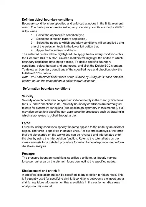
Defining object boundary conditionsBoundary conditions are specified and enforced at nodes in the finite element mesh. The basic procedure for setting any boundary condition except Contact is the same:1.Select the appropriate condition type.2.Select the direction (where applicable).3.Select the nodes to which boundary conditions will be applied usingone of the selection tools in the lower left button bar.4.Apply the boundary conditions.The selected nodes will be highlighted. To apply the boundary conditions click the Generate BCC's button. Colored markers will highlight the nodes to which boundary conditions have been applied. To delete specific boundary conditions, select the start and end nodes, and click the Delete BCC's button. To delete all boundary conditions of the specified type and direction, click the Initialize BCC's button.Note : You can either select faces of the surface by using the surface patches feature or use the node button to select individual nodes.Deformation boundary conditionsVelocityVelocity of each node can be specified independently in the x and y directions (or x, y, and z directions in 3d). Velocity boundary conditions are normally set to zero for symmetry conditions (see section on symmetry in this manual), but may also be set to a specified non-zero value for processes such as drawing in which a workpiece is pulled through a die.ForceForce boundary conditions specify the force applied to the node by an external object. The force is specified in default units. For die stress analysis, the force that the die exerted on the workpiece can be reversed and interpolated onto the dies by using the interpolation function. Refer to the tutorial labs on die stress analysis for a detailed procedure for using force interpolation to perform die stress analysis.PressureThe pressure boundary conditions specifies a uniform, or linearly varying, force per unit area on the element faces connecting the specified nodes. Displacement and shrink fitA specified displacement can be specified in any direction for each node. This is frequently used for specifying shrink fit conditions between a die insert and a shrink ring. More information on this is available in the section on die stress analysis in this manual.MovementThe movement of nodes on an object can be specified. If the movement boundary condition is specified, object movement controls must also be specified.ContactThe Contact boundary condition displays interobject boundary contact conditions on a given object. The user should gain some experience with DEFORM before using this option. The contact conditions are stored in three components to represent the fact that there are three degrees of freedom for any given node.ThermalHeat exchange with the environmentThis boundary condition specifies that heat exchange between element faces bounded by these nodes and their environment should occur. The contact boundary condition determines whether exchange will occur to the ambient atmosphere or to a contacting object.Heat fluxSpecifies an energy flux per unit area over the face of the element bounded by the nodes. Units are energy/time/area.Nodal heatSpecifies a heat source at the given nodes. Units are energy/time. TemperatureSpecifies a fixed temperature at the given nodes.Heat Exchange windowsThis function allows the user to define heat exchange conditions for local areas on a body by use of three dimensional window. To use heat exchange windows, perform the following actions:1.Go to the Boundary Conditions window.2.Select the Thermal tab.3.Select the Heat exchange windows button.4.Note the tools in the lower left corner of the display windowchanges and the new heat exchange window that comes up.5.At this point, heat exchange windows can be defined using the toolsin the lower left corner of the display window. Each window has its ownlocal environmental temperature, convection coefficient and emissivity.See Figure for an example heat exchange window.6.You can define up to 20 independent windows by the method. If tworegions share the same space, the lower number window wins. Diffusion [DIF]Diffusion with the environmentSpecifies diffusion of the dominant atom through the boundary elements bordered by the indicated nodes. Environment dominant atom content and surface reaction rate are specified under the Simulation Controls, Processing Conditions menu. Environment content and reaction rate for various regions of the part may be modified by using diffusion windows.Fixed atom contentSpecifies a fixed dominant atom content at the given nodes.Atom fluxSpecifies a fixed dominant atom flux rate over the elements bordered by the indicated nodes.2.4.11. Contact boundary conditionsContact boundary conditions are applied to nodes of a slave object, and specify contact between those nodes and the surface of a master object (see master-slave relationships under the Interobject data section). If a node is specified to be in contact with a particular object, it will placed on the surface of that object. If this requires changing the position of that node, it will be changed as necessary. Contact boundary conditions are generated under the InterObject , Contact Boundary Conditions.It is for this reason that the user should be VERY careful with how contact is specified. If it is improperly used, the mesh may be damaged and very often remeshing cannot aid this situation since the AMG cannot interpret the users intentions.Contact boundary conditions can be displayed for a given object using the Objects, Boundary Conditions, Advanced Deformation BCC's icon.。
Finite Element Analysis (FEA) Finite Element Analysis (FEA) is a powerful tool used in engineering to simulate and analyze the behavior of structures and components under various conditions. It is a numerical method that divides a complex system into smaller, simpler elements, allowing engineers to accurately predict how the system will respond to different loads and constraints. FEA has revolutionized the way engineers design and optimize structures, leading to safer, more efficient, and cost-effective solutions. One of the key benefits of FEA is its ability to simulate real-world conditions and scenarios that would be difficult or impossible to replicate in a physical test. By inputting material properties, boundary conditions, and loads into the FEA software, engineers can quickly analyze the stress, strain, and deformation of a structure, helping them identify potential failure points and optimize the design before manufacturing. This virtual testing not only saves time and resources but also reduces the risk of costly errors and failures in the field. FEA is widely used in various industries, including aerospace, automotive, civil engineering, and biomechanics, to name a few. In aerospace, FEA is used to analyze the structural integrity of aircraft components, ensuring they can withstand the extreme forces and vibrations experienced during flight. In automotive engineering, FEA helps optimize the design of vehicle components to improve performance, safety, and fuel efficiency. In civil engineering, FEA is used to analyze the stability of bridges, buildings, and other structures under different loading conditions. Despite its numerous advantages, FEA has its limitations and challenges. One of the main challenges is the accuracy of the results, which heavily depend on the input parameters, such as material properties and boundary conditions. Small errors in these parameters can lead to significant discrepancies in the simulation results, highlighting the importance of proper validation and verification of the FEA model. Additionally, FEA requires specialized training and expertise to use effectively, as well as powerful computing resources to handle the complex calculations involved in the analysis. Another important consideration when using FEA is the validation of the results through experimental testing. While FEA can provide valuable insights into the behavior of a structure, it is essential to validate the simulation resultsthrough physical testing to ensure the accuracy and reliability of the model. This iterative process of simulation and testing helps engineers refine their FEA models and improve the overall design of the structure. In conclusion, Finite Element Analysis is a valuable tool that has revolutionized the field of engineering by enabling engineers to simulate and analyze complex structures with accuracy and efficiency. While FEA offers numerous benefits, such as virtual testing, optimization, and cost savings, it also comes with challenges, such as accuracy, expertise, and validation. By understanding these limitations and best practices, engineers can harness the power of FEA to design safer, more reliable, and innovative structures that meet the demands of our modern world.。
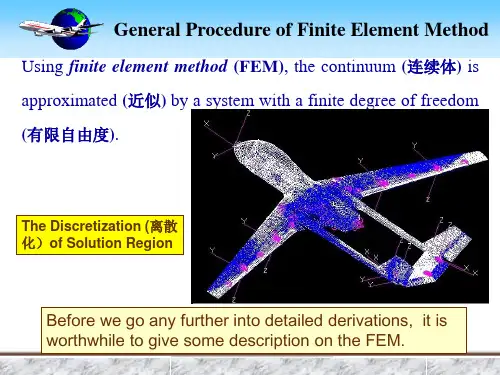
有限元仿真的英语Finite Element SimulationThe field of engineering has seen a remarkable evolution in recent decades, with the advent of advanced computational tools and techniques that have revolutionized the way we approach design, analysis, and problem-solving. One such powerful tool is the finite element method (FEM), a numerical technique that has become an indispensable part of the modern engineer's toolkit.The finite element method is a powerful computational tool that allows for the simulation and analysis of complex physical systems, ranging from structural mechanics and fluid dynamics to heat transfer and electromagnetic phenomena. At its core, the finite element method involves discretizing a continuous domain into a finite number of smaller, interconnected elements, each with its own set of properties and governing equations. By solving these equations numerically, the finite element method can provide detailed insights into the behavior of the system, enabling engineers to make informed decisions and optimize their designs.One of the key advantages of the finite element method is its abilityto handle complex geometries and boundary conditions. Traditional analytical methods often struggle with intricate shapes and boundary conditions, but the finite element method can easily accommodate these complexities by breaking down the domain into smaller, manageable elements. This flexibility allows engineers to model real-world systems with a high degree of accuracy, leading to more reliable and efficient designs.Another important aspect of the finite element method is its versatility. The technique can be applied to a wide range of engineering disciplines, from structural analysis and fluid dynamics to heat transfer and electromagnetic field simulations. This versatility has made the finite element method an indispensable tool in the arsenal of modern engineers, allowing them to tackle a diverse array of problems with a single computational framework.The power of the finite element method lies in its ability to provide detailed, quantitative insights into the behavior of complex systems. By discretizing the domain and solving the governing equations numerically, the finite element method can generate comprehensive data on stresses, strains, temperatures, fluid flow patterns, and other critical parameters. This information is invaluable for engineers, as it allows them to identify potential failure points, optimize designs, and make informed decisions that lead to more reliable and efficient products.The implementation of the finite element method, however, is not without its challenges. The process of discretizing the domain, selecting appropriate element types, and defining boundary conditions can be complex and time-consuming. Additionally, the accuracy of the finite element analysis is heavily dependent on the quality of the input data, the selection of appropriate material models, and the proper interpretation of the results.To address these challenges, researchers and software developers have invested significant effort in improving the finite element method and developing user-friendly software tools. Modern finite element analysis (FEA) software packages, such as ANSYS, ABAQUS, and COMSOL, provide intuitive graphical user interfaces, advanced meshing algorithms, and powerful post-processing capabilities, making the finite element method more accessible to engineers of all levels of expertise.Furthermore, the ongoing advancements in computational power and parallel processing have enabled the finite element method to tackle increasingly complex problems, pushing the boundaries of what was previously possible. High-performance computing (HPC) clusters and cloud-based computing resources have made it possible to perform large-scale, multi-physics simulations, allowing engineers to gain deeper insights into the behavior of their designs.As the engineering field continues to evolve, the finite element method is poised to play an even more pivotal role in the design, analysis, and optimization of complex systems. With its ability to handle a wide range of physical phenomena, the finite element method has become an indispensable tool in the modern engineer's toolkit, enabling them to push the boundaries of innovation and create products that are more reliable, efficient, and sustainable.In conclusion, the finite element method is a powerful computational tool that has transformed the field of engineering. By discretizing complex domains and solving the governing equations numerically, the finite element method provides engineers with detailed insights into the behavior of their designs, allowing them to make informed decisions and optimize their products. As the field of engineering continues to evolve, the finite element method will undoubtedly remain a crucial component of the modern engineer's arsenal, driving innovation and shaping the future of technological advancement.。
finite element modeler默认单位【原创版】目录1.Finite Element Modeling 简介2.Finite Element Modeler 默认单位3.默认单位的影响4.如何更改默认单位5.总结正文1.Finite Element Modeling 简介有限元建模(Finite Element Modeling)是一种数值分析方法,它通过将结构分解为许多小的、简单的部分(称为元素),然后对这些元素进行求解,最终得到整个结构的解。
这种方法被广泛应用于工程领域,如结构分析、热传导、流体力学等。
2.Finite Element Modeler 默认单位有限元建模器(Finite Element Modeler)是进行有限元分析的软件工具。
在使用这些软件时,我们通常需要关注的一个重要参数是单位的设置。
Finite Element Modeler 的默认单位是英制单位,即英里、英尺、英寸等。
3.默认单位的影响使用默认单位可能会对模型的精度和结果产生影响。
例如,当我们模拟一个结构时,如果单位设置不正确,可能会导致计算结果不准确,从而影响我们的分析和设计。
4.如何更改默认单位如果需要更改 Finite Element Modeler 的默认单位,可以按照以下步骤操作:(1)打开有限元建模软件,进入“文件”(File)菜单,选择“单位”(Units)选项。
(2)在弹出的“单位”(Units)对话框中,选择“公制”(Metric)作为单位制。
(3)点击“确定”(OK)按钮,完成单位设置。
5.总结在使用 Finite Element Modeler 进行有限元建模时,我们需要关注单位的设置,确保使用正确的单位制。
如果需要更改默认单位,可以通过上述步骤进行操作。
finite element procedures inengineering analysisFinite element procedures, also known as finite element analysis (FEA), are numerical techniques used in engineering analysis to simulate and solve complex problems involving structures, mechanical systems, and other physical phenomena. These procedures are based on the discretization of a continuum or a geometrical domain into a finite number of elements, interconnected at nodes.The primary goal of finite element procedures is to predict the behavior of a system under various loading conditions and boundary constraints. By breaking down the problem into smaller elements, the equations governing the behavior of the system can be formulated and solved using matrix-based numerical methods.One of the key advantages of finite element procedures is their ability to handle complex geometries and boundary conditions. They can be applied to structures with irregular shapes, holes, or curved surfaces, which would be challenging to analyze using traditional analytical methods. Additionally, finite element procedures allow for the simulation of a wide range of physical phenomena, including structural deformation, heat transfer, fluid flow, and electromagnetic fields.During the finite element analysis, a mesh is generated, which represents the discretized domain. The mesh consists of elements with defined shapes, such as triangles or quadrilaterals in 2D and tetrahedra or hexahedra in 3D. The nodes at the intersections of elements serve as points where the system's unknown variables, such as displacements or temperatures, are defined.Once the mesh is created, the governing equations, such as the equilibrium equations in structural analysis or the heat conduction equation in thermal analysis, are formulated for each element. These equations are then assembled into a global system of equations, which can be solved using numerical techniques, such as the Gaussian elimination or iterative methods.The results of the finite element analysis provide valuable insights into the behavior of the system, including stress distributions, deformations, temperature gradients, or fluid velocities. These results can be visualized d and analyzed to assess the performance, reliability, and safety of engineering designs.In summary, finite element procedures are essential tools in engineering analysis, allowing engineers to simulate and predict the behavior of complex systems with high accuracy. These procedures provide valuable insights into the performance and design优化 of various engineering structures and phenomena.。
Finite Elements in Analysis and Design43(2007)589–598/locate/finelEquivalent axial stiffness of various components in bolted jointssubjected to axial loadingFeras Alkatan,Pierre Stephan,Alain Daidie∗,Jean GuillotLaboratory of Mechanical Engineering of Toulouse,135Rangueil Avenue,31077Toulouse,Cedex04,FranceReceived27June2006;received in revised form18December2006;accepted30December2006Available online7March2007AbstractManaging the axial stiffness of various components in a bolted joint is a major industrial concern for modelling different tightening processes and for accurate fatigue dimensioning.This paper presents a new approach for calculating the axial stiffness of the several elements of a bolt(the head and the engaged part),the nut and the fastened plates.Finite element modelling based on deformation energy improves the existing models and take in to account the type of materials and coefficients of friction of various elements in contact.From these corrections, approaches for axial stiffness calculation based on empirical formulas are proposed for easier application and for future FE modelling bolted joints using beam elements.Finally,the theoretical study is validated by an original experimental approach.᭧2007Elsevier B.V.All rights reserved.Keywords:Bolted joint;Angle-controlled tightening;Axial stiffness;Bolt;Nut;Tapping;Contact;Modelling;Finite elements1.IntroductionStiffness of the subassemblies in a bolted joint reflects the overall behaviour of the assembly subjected axial loading which is mainly displacement along the axis of the bolts.Thus,man-aging the equivalent stiffness of the bolt,the nut and sub-assemblies is necessary for dimensioning in fatigue,modelling the tightening process and investigating the behaviour of these assemblies under thermal stresses.The1986VDI2230recommendation which is the most fre-quently used in industrial calculations and specialised research works like those developed by Bickford and Nassar[1],Guillot [2]was always questionable[3]and even completely modified in some references like the2003VDI2230[4].A benchmark of developed approaches anterior to1990can be found in Lenhoff et al.[5].However,it was the development offinite elements which led up to more accurate models.One should note that the main objective remains displacement along the axis of the bolt. In this framework,Wileman et al.[6]considered the washer as ∗Corresponding author.Tel.:+33561559731;fax:+33561559950.E-mail address:alain.daidie@insa-toulouse.fr(A.Daidie).0168-874X/$-see front matter᭧2007Elsevier B.V.All rights reserved. doi:10.1016/j.finel.2006.12.013a rigid body in simulating the interaction between the head of the bolt and the part.Unfortunately,this approach appeared to be irrealistic and inaccurate as shown by Guillot[3],Massol[7] and Zadoks[8].Lehnhoff et al.[5,9,10]calculated an average equivalent displacement for the nodes at the contact zone to simulate this interaction.To validate this approach,Massol[7]conducted experimen-tal measurements.Unfortunately,it was difficult to accurately determine the deformation of the subassemblies along the assembly axis.Thus,the results seemed mediocre.In this paper,a new approach for stiffness calculation is pre-sented:this approach takes into account the various geomet-rical parameters,the coefficient of friction and the materials properties in the case of axisymmetric loading.Three-dimensionalfinite elements(FEM)are conducted to calculate the apparent stiffness of the subassemblies using the deformation energy method.Then,results are compared to previous studies and validated by an original experimental approach.Finally,the various ratios necessary for stiffness calculation are integrated in an empirical formula that can be easily pro-grammable in a tool for industrial design office use.590F.Alkatan et al./Finite Elements in Analysis and Design43(2007)589–598 NomenclatureA d3thread root area(mm2)A p equivalent cross-section of fastened parts(mm2)A∗p dimensionless equivalent cross-section of fas-tened partsA s bolt stress area(mm2)A0bolt nominal cross-section(mm2)D nut nominal diameter(mm)d bolt nominal diameter(mm)D a diameter under bolt head(mm)D ext nut external diameter(mm)D p fastened plates diameter(mm)D∗p fastened plates dimensionless diameterD t bolt hole diameter(mm)D∗t bolt hole dimensionless diameterE bolt bolt modulus of elasticity(N/mm2)E head bolt head modulus of elasticity(N/mm2)E nut nut modulus of elasticity(N/mm2)E part fastened plates modulus of elasticity(N/mm2)E tapping tapped part modulus of elasticity(N/mm2)F tot applied axial load(N)H nut standardised height(mm)h height of bolt head(mm)K bolt.nut stiffness of the nut and engaged part of the bolt (N/mm)K head bolt head stiffness(N/mm)K p stiffness of fastened parts(N/mm)K∗p dimensionless stiffness of fastened partsK tapping stiffness of a tapped hole(N/mm)K bolt.tapping tapped hole and thread stiffness(N/mm) L p height of bolted parts(mm)L∗p dimensionless height of bolted partsL0length of bolt cylindrical part(mm)L1length of bolt threaded part(mm)p pitch of thread(mm)W e nut deformation energy induced in the nut(N mm)W e part deformation energy induced in the boltedparts(N mm)bolt correcting factor of the engaged part of theboltbolt.nut stiffness correcting factor of the nut and theengaged part of the boltbolt.tapping stiffness correcting factor of a tapped holeand the engaged part of the bolthead stiffness correcting factor of the bolt head threaded stiffness correcting factor of the boltthreaded parttapping stiffness correcting factor of a tapped hole 0displacement due to clamping(on preload-ing F0)(mm)coefficient of frictioneq equivalent coefficient of friction1coefficient of friction between the bolt andthe nut2coefficient of friction between the nut andthe fastened platestightening angle(degrees)2.Problem set up2.1.General approachIn the aim of developing a new general calculation method, the overall assembly is partitioned into functional parts:the threaded portion of the bolt,the bolt head,the threads engaged in the nut,the fastened plates and the threads engaged in the tapped subassembly(see Fig.1).The local approach consists of calculating the local rigidity of each of these functional parts. It is then extended to a more global approach to calculate the global stiffness of the bolted assembly.This classical approach is similar to the one used in VDI2230recommendation[11].2.2.Calculation of the equivalent stiffnessEach subassembly is assimilated to a spring with an equiv-alent stiffness(see Fig.3).Fromfinite element analysis,one can conclude(see Fig.3a)that under loading,the displacement of the upper part of the screw( )is proportional to the ap-plied load F[12].Calculating the stiffness K B and K p of each element apart is justified since due to local deformations at the interface head-part,it is difficult to accurately estimate the displacement along the axis,and consequently the length vari-ation(see Fig.2).Using the elastic deformation energy for each element,the equivalent stiffness can be deduced.Applying the principle of energy conservation to the considered system(see Fig.2a),and considering a free unfrictional contact in the rigid plane(x,z): 12F =W B+W p+W f,(1) where W B is the elastic deformation energy of the bolt,W p the elastic deformation energy of the part,W f the dissipatedfrictional energy at the interface head-part,and12F the work of the external forces.Consequently,the two cases which can be investigated are presented below.2.2.1.Unfrictional contact under head12F =W B+W p.(2) Since thefinite elements model show a linear behaviour,the stiffness of the springs can be calculated using the following relations:K B=F22W Band K p=F22W p.(3)F .Alkatan et al./Finite Elements in Analysis and Design 43(2007)589–598591fastened plates dFig.1.Definition of the various functional parts in a bolted joint.0.00−0.02−0.04−0.06−0.10−0.12−0.14−0.16−0.18−0.20−0.08Y Z XFig.2.Displacement of the loaded assembly (mm).This approach which neglects the frictional energy loss (W f )at the contact interface head-part can be considered satisfactory since for a standardised cylindrical head screw and for t =0.2the difference between the total calculated flexibility (S T =1/K B +1/K p )and the “measured”flexibility S = /F is less than 2%[12].2.2.2.Frictional contact under headFor a frictional contact at the interface head-part,the direc-tion of the contact forces is modified and consequently W B and W p since as shown in Eq.(4),mechanical energy is dissipated in the slipping area:W f =12F −(W B +W p ).(4)F is calculated by summing local values (F i i )at the nodesof the contact section.W B and W p are the software outputs set out by summing the elastic deformation energy of each element.One should note that the “springs”model (see Fig.3b)does not simulate the frictional energy loss.However,the equivalent axial stiffness K B and K p associated to the deformation energiesof the springs W B and W pcan be deduced using the followingModel of finite elements simulationEquivalent calculation modelFig.3.Definition of the equivalent model.relation:W B +W p +W f =12F =W B +W p .(5)It can be easily verified that the frictional lost energy isproportional to the elastic deformation energy,thus:12F =W B+W p = (W B +W p ),(6)592F.Alkatan et al./Finite Elements in Analysis and Design43(2007)589–598Fig.4.Digital calculation equivalent models.Bolt NutWe nutWeAssembled partContactregions3rzFig.5.Finite element meshing of the various regions.where,=F2(W B+W p).(7)From Eq.(3),one can deduce:K B=F22W Band K p=F22W p,(8)whereW B= W B and W p= W p.(9)From(7–9):K B=F1+W pW B,(10)K p=F1+W BW p.(11)Consequently,the equivalent stiffness K B K p is calculated byextracting out(W B,W p,F, )from thefinite element simula-tion.This approach is advantageous since it does not requiredisplacement along the axis.Besides,it is simple and accuratesince the elastic deformation energy is precisely estimated withthefinite element software.2.3.ModellingThefinite element model was developed under thefiniteelement software I-DEAS[13].The effects induced by thehelix angle are ignored since this angle has negligible effect onthe load distribution between the engaged threads as shown byFukuoka et al.[14]and Zhao[15].Two types of meshing wereinvestigated:a free meshing using10nodes linear bricks anda mapped meshing with eight nodes bricks elements.The lat-ter was retained since it generates a better element repartitionin the assembly and can be more advantageous for comparisonbetween different simulations and resolving contact problems.An axisymmetric model is considered and the study isreduced to an angular portion of3◦since a preliminary studyon various angle sectors showed that starting from a portion of3◦the results are identical.This meshing is parametrised withthe geometry of the model as shown in Fig.4.The contact be-haviour at the interfaces of the threads and at the nut-fastenedplates can be defined independently from the mesh(seeFig.5).The boundary conditions are defined on the assem-bly geometry in a cylindrical coordinate system(see Fig.5).Radial translations along the radial faces of the screw,the nutand the assembled parts are restrained( =0).The bottom ofan assembled part is also restrained in displacement along z-axis and the preload is applied by a imposed displacement( )F .Alkatan et al./Finite Elements in Analysis and Design 43(2007)589–598593at the bottom of the fixation.This approach is advantageous since several dimensional cases can be rapidly investigated.3.Results and analysis3.1.Stiffness of the bolt’s elementsCorrecting factors are used to assimilate the threaded part,the nut and tapping to the equivalent length of a cylindrical bar with cross-sections A s and A 0for the bolt head.Fig.6shows the current method [2,16]and the new modified model which takes into consideration the influence of the threads,the head,and the part in bolt–nut contact.The correcting factors are given by bolt .nut =E bolt ·A sd ·K bolt .nut ,(12a) tapping =E tapping ·A sd ·K tapping,(12b) thread =E bolt ·A sL ·K thread,(12c) head =E bolt ·A 0d ·K head.(12d)3.2.Stiffness of threaded portion of the boltMany studies were conducted concerning the stiffness of the threaded portion of the bolt (see Fig.6),which is classically assimilated to an equivalent section A eq equal to the resistant section [2,11].The purpose of this study is to refine this value by a weighting factor tread which corrects the threaded length L 1without modifying the defined equivalent section.Using the deformation energy method of several values for the undimensionless parameter p/d for large and fine pitch screws (see Fig.7),brings up results very close to those ob-tained in Section 1:the maximum relative variations,for sig-nificant values of p/d are around 4.5%.Consequently,the traditional use of an equivalent section is justified.Practically,identical values are obtained for threebolt new calculation modelinitial calculation modelαhead .d.L 1α.dor.ddab cFig.6.Calculation models relating to the bolt.types of materials,independently from the type of pitch.The evolution of the ratio A s /A eq with p/d is almost linear.The coefficient thread refines the equivalent length of the threaded part for fine and large pitch screw.Thus,a valid formulation for all types of screw is given: thread =A s A eq =0.956+0.534pd.(13)3.3.Stiffness of the bolt’s headMany studies have been conducted on the stiffness of thebolts head [7].In this framework,German rules VDI 2230[4,11]recommend a corrective factor equal to 0.4whereas Mas-sol [7]introduced a ratio head related to the geometry.This study assumes perfect adherence and does not take into con-sideration the sliding of the head on the fastened plates and consequently markedly modifies the zone of load introduction.Results presented in this paper show a weak influence of the nominal diameter of the bolt and the diameter of the subassem-blies.Note that the correcting factor is about 4%greater for a coefficient of friction close to 0.For a standardised head height,the influential parameters are the diameter of the tapped hole and the subassemblies materials (see Fig.8).For a coefficient of friction =0.2and a standardised head height (h =0.65d),the ratio head is given byhead =0.47+ d t −1.05dd −0.04E part E bolt −1 .(14)During the tightening process,radial deformation is set freeas if the “radial”coefficient of friction is equal to zero [12].Thus,the ratio head given by the empirical formula (14)should be increased about 3%whereas for a head height equal to the nominal diameter (optimum bolt head stiffness [12]),this ratio must be increased around 6%.3.4.Stiffness of the nut and the engaged part of the bolt It is important to accurately determine the axial stiffness of the nut since it dispatches the entire load through the bolt to the assembly Sawa and Maruyama [17]proposed a value of594F.Alkatan et al./Finite Elements in Analysis and Design43(2007)589–598the bolt.nut factor equal to0.7based on theoretical3D studiesand experimental results.From afinite element results,Fukuoka[18]suggests a valueof1.05for a coefficient of friction equal to0and0.65for acoefficient of friction equal to0.4.However,he recommendsa mean value equal to0.85.Recently,Guillot[2]proposed avalue of1.1d instead of0.4d(see Fig.6)to take into accountthe stiffness of the threads.Genelot[19]validated this proposalfor low coefficients of friction and large hole diameters.Note that the German VDI recommendation[4]distinguishesbetween the rigidity K bolt of the portion of the bolt inside thenut and the rigidity K nut of the nut itself:K bolt=E bolt·A d30.5dfor bolt=0.5,(15)K nut=E nut·A00.4dfor nut=0.4.(16)For two identical materials, bolt.nut=0.85.This value isequal to the mean value suggested by Fukuoka[18].This paper shows a relatively low influence of the nominaldiameter especially for a low coefficient of friction.Thus,amean value is considered for the range of diameters between6and36mm.A s/Aéq0.9811.021.041.060.070.090.110.130.150.17p/dmon function of variation of A s/A eq coefficient according top/d report ratio.M20 ; h/d = 0.65 ; μ = 0.2 ; D t = 210.40.50.60.70.80.30.8 1.3 1.8αheadE part/E boltM20 ; h/d = 0.65 ; μ = 0.2 ; steel/steel0.20.30.40.50.60.70.8αhead(D t-d)/dFig.8. head ratio in relation to the relative radial clearance(D t−d)/d and the moduli of elasticity ratio E part/E bolt.The evolution of bolt.nut with the elasticity coefficients ofmaterials is practically linear(see Fig.9b).Concerning thecoefficient of friction,the bolt.nut decreases for =0.23andthen remains constant.For a bolt and a nut made of the same material,the valuerecommended by Guillot is found for =0and bolt.nut=1.1.This value can be used in the case of torque tightening,sinceorthoradial sliding yields to a free distension of the nut andthus to a theoretical coefficient of friction equal to0[12].The mean value g bolt.nut=0.85recommended by VDI[4]Fukuoka[18]is also found.Finally,these results lead to amore general empirical formulation that takes into account thecoefficient of friction and the ratio of elasticity coefficients:For0 0.23:bolt.nut=A−B. ,(17)whereA=1.1+E boltE nut−10.54B=1.65+E boltE nut−11.2For 0.23:bolt.nut=0.71+E boltE nut−10.25.(18)One should know that friction coefficients bolt–nut 1andnut-fastened plates 2do not have the same influence sinceresults show that the latter contributes around60%in the cal-culation of bolt.nut.Consequently,an equivalent coefficient offriction is given byeq=2 1+3 25.(19)3.5.Stiffness of a tapped partNumerous studies,based on experimental and digital tests,have been conducted to investigate local behaviour at the threadand Design43(2007)589–59859500.10.20.30.4μ=00.611.41.82.2E bolt/E nutαbolt-nutμFig.9.Correcting factor bolt.nut in relation to the coefficient of friction :(a)and the moduli of elasticity ratio E bolt/E nut;(b)for a standardised nut.M16 ; μ=0 ; Dextvariable0.750.850.951.051.15M16 ; μ=0 ; H variable0.750.850.951.051.1524446484104ααFig.10.Correcting factor in relation to the height and external diameter of a non-standardised nut.root[8,14]to define the fatigue resistance and evaluate the max-imum stress taking into consideration the probability of localplastification.However,the main objective remains the equiv-alent local stiffness of the portion of the bolt engaged in thetapped hole(see Fig.5).VDI recommendation[4]and Thomala[20]are the only ones to give results for fastened plates.In thisframework,a preliminary study of nuts with different heightsand diameters showed that the correcting factor remains some-how constant with large height and diameter of tapped parts(see Fig.10).Consequently,for stiffness calculation,one canconsider:H=3H standardised and D ext=5D a.One should note that the portion of a bolt in a tapping is amajor constructive datum.However,a recent investigation[12]showed that the stiffness of a tapped part barely varies for morethan seven engaged threads as shown by the results below,setout from a study in the elastic range.Practically,some threadsmay plastify and consequently lead to a more uniform loaddistribution:a study covering this phenomenon is actually underdevelopment.Since in the elastic domain,the coefficient bolt.tapping barelyvaries with the nominal diameter,specifically for low coeffi-cients of friction,it would be accurate to consider the meandiameter.The curves presented in Fig.11match with the results of theprevious study.One can conclude that the coefficient of frictionand the materials are less influential.This can be justified sincethe considered part has a large diameter,and thus the radialdeformations near the threading are negligible independentlyfrom the coefficient of friction and the material.Hence,the following empirical formula is presented:For0 0.33:bolt.tapping=A−B. ,(20)whereA=0.78+E boltE tapping−10.21,B=0.27+E boltE tapping−10.15.For 0.33:bolt.tapping=0.7+E boltE tapping−10.16.(21)Note that the objective of this study is to determine thestiffness of the engaged portion of the bolt and the tapped596F .Alkatan et al./Finite Elements in Analysis and Design 43(2007)589–5980.60.70.80.911.11.200.10.20.30.40.5μ20.60.811.21.411.522.53E bolt /E tappingαb o l t -t a p p i n gαb o l t -t a p p i n gFig.11.Correcting factor tapping in relation to the coefficient of friction between threads 2and the moduli of elasticity ratio E bolt /E tapping .L definition of assembled partsequivalent model withsame stiffnesspFig.12.Equivalent calculation model of the fastened plates axial stiffness.part with large dimensions.However,concerning the area be-tween the standardised nut (H nut -N ;D ext nut -N )and the part (H ;D ext ),a general model using the previously defined co-efficients bolt .tapping and bolt .nut and based on the results of Fig.11is used.Eq.(22)represents the generalised model for: bolt .nut < < bolt .tapping .= bolt .tapping +13 0.8d/H2−0.8d/H+23 1.15d/D ext 4−3.45d/D ext( bolt .nut − bolt .tapping ).(22)3.6.Stiffness of fastened platesUnder uniform load,the apparent stiffness of a part with an equivalent cross-section A p and a length L p (equal to the length of the assembly),is equivalent to the stiffness of fastened plates as shown in Fig.12.For each subassembly,the equivalent cross-section is de-duced from the compression stiffness using the following rela-tion:A p =L p ·K pE part.(23)Consequently,the equivalent undimensionless cross-section is A ∗p =A pD 2a,where D a is the diameter of the bolt head.The various geometrical magnitudes of the bolted joint are also defined in relation to D a by the following relations:D ∗p =D pD a;D ∗t =D tD a;L ∗p =L pD a.(24)As previously mentioned,numerous studies concerning the equivalent stiffness of fastened plates were conducted.The most interesting approach is based on the notion of a deformation cone with the same stiffness as the subassemblies [5,11].This description features an assembly of parts with different diam-eters by a purely geometric approach.Consequently,the angle of the cone,considered as an additional geometric parameter is related to the various characteristics of the assembly [21–23]by various empirical relations.For cylindrical parts with the same diameter,Rasmussen [24]presents an empirical formula (24)which was modified by Massol [2,7]and used by Vadean [16].This formula is consistent since it gives satisfactory results for a coefficient of friction close to 0(see Fig.13).A ∗p =4(1−D ∗2t )+12(D ∗2p −1)×tan−1⎡⎢⎣0.35L ∗p+1+2L ∗2p −12(D ∗2p −D ∗2t)⎤⎥⎦,(25)A ∗p =4(1−D ∗2t )+12(D ∗2p−1)tan −10.75(L ∗p −0.2)(D ∗2p −D ∗2t) .(26)A full experimental design study covering a broad domain (1 D ∗p 5;0.02 L ∗p10)shows that the equivalent cross-section scarcely depends on the nominal diameter of the bolt.In fact,the influential parameters are the contact diameter of the bolt head,thickness and diameter of the fastened plates andF .Alkatan et al./Finite Elements in Analysis and Design 43(2007)589–5985970.20.40.60.811.21.41.61.8212345FEM_μ=0Rasmussen (25)Formula (26)VDI_03FEM_μ=0.2M24 ; L p *=3.330123450246810FEM_µ=0Rasmussen (25)A p *_VDI_03Formula (26)D p *=5 ; d t =25 mmA p *A p *D p *L p *Fig.13.Equivalent cross-section in relation to the dimensions of the part.the radial clearance at the hole.The coefficient of friction also has a light influence on A ∗p (from 5%to 10%).The Rasmussen formulation is modified and an easy ex-pression for A p (Eq.(26))covering the case of thin parts and a coefficient of friction close to 0.2at the interfaces is developed.This formula covers most industrial cases and highlights the influence of the various parameters.One can also deduce from this study that A p does not depend on the materi-als of the bolt and the fastened plates.Finally,a simple method for extending this formulation for stacked parts with different diameters and materials will be presented in a forthcoming publication.4.Experimental validationThe aim of the experimental validation is to determine the stiffness of the subassemblies in the bolted joint.In the ex-perimental set-up shown in Fig.14,a tightening torque is ap-plied on the nut for measuring the screwing angle whereas two deformation gauges and two rosette gauges are,respectively,installed on the bolt to measure the axial tension and torsional moment.However,it is practically impossible to perform a direct measurement on the length variation of the subassem-blies.However,even if these assemblies are made of steel or light alloy and thus variations are extremely slight,the length variation of the bolt’s axis is not really materialised and there-fore remains not accessible for direct measurement.The experimental approach is based on the assumption of the linear variation of stiffness with Young modulus of elasticity and loading.Thus,a double measurement is performed using a batch of steel parts having an modulus of elasticity E p1and a batch of aluminium parts with a modulus of elasticity E p2hav-ing the same geometry.This approach was used by Massol [7]in FEM simulations.The relative imposed displacement gener-ates,respectively,a load F 1and F 2in the steel and aluminium parts.F 1and F2are measured in the linear part of the curve,thus giving the load relatively to the screwing angle (see Fig.15),for given.Blocked bolt headTightening torque applied tothe nut Angle tightening measurement Cylindrical partof boltRigid supportTop view of systemFig.14.Equivalent cross-section in relation to the dimensions of the part.From Eq.(27),the stiffness of the bolt (Eq.(28))and the equivalent undimensionless cross-section A ∗p Eq.(29)characteristic of the stiffness of the fastened plates can be deduced:=P2 =F i 1K B +1K p1 ,(27)K B =F 1−F 2L p /A p (F 2/E p21/E p1),(28)A ∗p =L p D a (1/E p2−1/E p1)(1/F 21).(29)The experimental results validate the Rasmussen modifiedformula (see Fig.(16))where the axial stiffness of the bolt is set out by summing the flexibility of the various elements.The relative error is less than 8%.。
The finite element analysisFinite element method, the solving area is regarded as made up of many small in the node connected unit (a domain), the model gives the fundamental equation of sharding (sub-domain) approximation solution, due to the unit (a domain) can be divided into various shapes and sizes of different size, so it can well adapt to the complex geometry, complex material properties and complicated boundary conditionsFinite element model: is it real system idealized mathematical abstractions. Is composed of some simple shapes of unit, unit connection through the node, and under a certain load.Finite element analysis: is the use of mathematical approximation method for real physical systems (geometry and loading conditions were simulated. And by using simple and interacting elements, namely unit, can use a limited number of unknown variables to approaching infinite unknown quantity of the real system.Linear elastic finite element method is a ideal elastic body as the research object, considering the deformation based on small deformation assumption of. In this kind of problem, the stress and strain of the material is linear relationship, meet the generalized hooke's law; Stress and strain is linear, linear elastic problem boils down to solving linear equations, so only need less computation time. If the efficient method of solving algebraic equations can also help reduce the duration of finite element analysis.Linear elastic finite element generally includes linear elastic statics analysis and linear elastic dynamics analysis from two aspects. The difference between the nonlinear problem and linear elastic problems:1) nonlinear equation is nonlinear, and iteratively solving of general;2) the nonlinear problem can't use superposition principle;3) nonlinear problem is not there is always solution, sometimes even no solution. Finite element to solve the nonlinear problem can be divided into the following three categories:1) material nonlinear problems of stress and strain is nonlinear, but the stress and strain is very small, a linear relationship between strain and displacement at this time, this kind of problem belongs to the material nonlinear problems. Due to theoretically also cannot provide the constitutive relation can be accepted, so, general nonlinear relations between stress and strain of the material based on the test data, sometimes, to simulate the nonlinear material properties available mathematical model though these models always have their limitations. More important material nonlinear problems in engineering practice are: nonlinear elastic (including piecewise linear elastic, elastic-plastic and viscoplastic, creep, etc.2) geometric nonlinear geometric nonlinear problems are caused due to the nonlinear relationship between displacement. When the object the displacement is larger, the strain and displacement relationship is nonlinear relationship. Research on this kind of problemIs assumes that the material of stress and strain is linear relationship. It consists of a large displacement problem of large strain and large displacement little strain. Such as the structure of the elastic buckling problem belongs to the large displacement little strain, rubber parts forming process for large strain.3) nonlinear boundary problem in the processing, problems such as sealing, the impact of the role of contact and friction can not be ignored, belongs to the highly nonlinear contact boundary.At ordinary times some contact problems, such as gear, stamping forming, rolling, rubber shock absorber, interference fit assembly, etc., when a structure and another structure or external boundary contact usually want to consider nonlinear boundary conditions. The actual nonlinear may appear at the same time these two or three kinds of nonlinear problems.Finite element theoretical basisFinite element method is based on variational principle and the weighted residual method, and the basic solving thought is the computational domain is divided into a finite number of non-overlapping unit, within each cell, select some appropriate nodes as solving the interpolation function, the differential equation of the variables in the rewritten by the variable or its derivative selected interpolation node value and the function of linear expression, with the aid of variational principle or weighted residual method, the discrete solution of differential equation. Using different forms of weight function and interpolation function, constitute different finite element methods. 1. The weighted residual method and the weighted residual method of weighted residual method of weighted residual method: refers to the weighted function is zero using make allowance for approximate solution of the differential equation method is called the weighted residual method. Is a kind of directly from the solution of differential equation and boundary conditions, to seek the approximate solution of boundary value problems of mathematical methods. Weighted residual method is to solve the differential equation of the approximate solution of a kind of effective method.Hybrid method for the trial function selected is the most convenient, but under the condition of the same precision, the workload is the largest. For internal method and the boundary method basis function must be made in advance to meet certain conditions, the analysis of complex structures tend to have certain difficulty, but the trial function is established, the workload is small. No matter what method is used, when set up trial function should be paid attention to are the following:(1) trial function should be composed of a subset of the complete function set. Have been using the trial function has the power series and trigonometric series, spline functions, beisaier, chebyshev, Legendre polynomial, and so on.(2) the trial function should have until than to eliminate surplus weighted integral expression of the highest derivative low first order derivative continuity.(3) the trial function should be special solution with analytical solution of the problem or problems associated with it. If computing problems with symmetry, should make full use of it. Obviously, any independent complete set of functions can be used as weight function. According to the weight function of the different options for different weighted allowance calculation method, mainly include: collocation method, subdomain method, least square method, moment method and galerkin method. The galerkin method has the highest accuracy.Principle of virtual work: balance equations and geometric equations of the equivalent integral form of "weak" virtual work principles include principle of virtual displacement and virtual stress principle, is the floorboard of the principle of virtual displacement and virtual stress theory. They can be considered with some control equation of equivalent integral "weak" form. Principle of virtual work: get form any balanced force system in any state of deformation coordinate condition on the virtual work is equal to zero, namely the system of virtual work force and internal force ofthe sum of virtual work is equal to zero. The virtual displacement principle is the equilibrium equation and force boundary conditions of the equivalent integral form of "weak"; Virtual stress principle is geometric equation and displacement boundary condition of the equivalent integral form of "weak". Mechanical meaning of the virtual displacement principle: if the force system is balanced, they on the virtual displacement and virtual strain by the sum of the work is zero. On the other hand, if the force system in the virtual displacement (strain) and virtual and is equal to zero for the work, they must balance equation. Virtual displacement principle formulated the system of force balance, therefore, necessary and sufficient conditions. In general, the virtual displacement principle can not only suitable for linear elastic problems, and can be used in the nonlinear elastic and elastic-plastic nonlinear problem.Virtual mechanical meaning of stress principle: if the displacement is coordinated, the virtual stress and virtual boundary constraint counterforce in which they are the sum of the work is zero. On the other hand, if the virtual force system in which they are and is zero for the work, they must be meet the coordination. Virtual stress in principle, therefore, necessary and sufficient condition for the expression of displacement coordination. Virtual stress principle can be applied to different linear elastic and nonlinear elastic mechanics problem. But it must be pointed out that both principle of virtual displacement and virtual stress principle, rely on their geometric equation and equilibrium equation is based on the theory of small deformation, they cannot be directly applied to mechanical problems based on large deformation theory. 3,,,,, the minimum total potential energy method of minimum total potential energy method, the minimum strain energy method of minimum total potential energy method, the potential energy function in the object on the external load will cause deformation, the deformation force during the work done in the form of elastic energy stored in the object, is the strain energy.The convergence of the finite element method, the convergence of the finite element method refers to when the grid gradually encryption, the finite element solution sequence converges to the exact solution; Or when the cell size is fixed, the more freedom degree each unit, the finite element solutions tend to be more precise solution. Convergence condition of the convergence condition of the finite element finite element convergence condition of the convergence condition of the finite element finite element includes the following four aspects: 1) within the unit, the displacement function must be continuous. Polynomial is single-valued continuous function, so choose polynomial as displacement function, to ensure continuity within the unit. 2) within the unit, the displacement function must include often strain. Total can be broken down into each unit of the state of strain does not depend on different locations within the cell strain and strain is decided by the point location of variables. When the size of the units is enough hours, unit of each point in the strain tend to be equal, unit deformation is uniform, so often strain becomes the main part of the strain. To reflect the state of strain unit, the unit must include the displacement functions often strain. 3) within the unit, the displacement function must include the rigid body displacement. Under normal circumstances, the cell for a bit of deformation displacement and displacement of rigid body displacement including two parts. Deformation displacement is associated with the changes in the object shape and volume, thus producing strain; The rigid body displacement changing the object position, don't change the shape and volume of the object, namely the rigid body displacement is not deformation displacement. Spatial displacement of an object includes three translational and three rotational displacement, a total of six rigid body displacements. Due to a unit involved in the other unit, other units do rigid body displacement deformation occurs willdrive unit, thus, to simulate real displacement of a unit, assume that the element displacement function must include the rigid body displacement. 4) the displacement function must be coordinated in public boundary of the adjacent cell. For general unit of coordination is refers to the adjacent cell in public node have the same displacement, but also have the same displacement along the edge of the unit, that is to say, to ensure that the unit does not occur from cracking and invade the overlap each other. To do this requires the function on the common boundary can be determined by the public node function value only. For general unit and coordination to ensure the continuity of the displacement of adjacent cell boundaries. However, between the plate and shell of the adjacent cell, also requires a displacement of the first derivative continuous, only in this way, to guarantee the strain energy of the structure is bounded. On the whole, coordination refers to the public on the border between neighboring units satisfy the continuity conditions. The first three, also called completeness conditions, meet the conditions of complete unit is complete unit; Article 4 is coordination requirements, meet the coordination unit coordination unit; Otherwise known as the coordinating units. Completeness requirement is necessary for convergence, all four meet, constitutes a necessary and sufficient condition for convergence. In practical application, to make the selected displacement functions all meet the requirements of completeness and harmony, it is difficult in some cases can relax the requirement for coordination. It should be pointed out that, sometimes the coordination unit than its corresponding coordination unit, its reason lies in the nature of the approximate solution. Assumed displacement function is equivalent to put the unit under constraint conditions, the unit deformation subject to the constraints, this just some alternative structure compared to the real structure. But the approximate structure due to allow cell separation, overlap, become soft, the stiffness of the unit or formed (such as round degree between continuous plate unit in the unit, and corner is discontinuous, just to pin point) for the coordination unit, the error of these two effects have the possibility of cancellation, so sometimes use the coordination unit will get very good results. In engineering practice, the coordination of yuan must pass to use "small pieces after test". Average units or nodes average processing method of stress stress average units or nodes average processing method of stress average units or nodes average processing method of stress of the unit average or node average treatment method is the simplest method is to take stress results adjacent cell or surrounding nodes, the average value of stress.1. Take an average of 2 adjacent unit stress. Take around nodes, the average value of stressThe basic steps of finite element method to solve the problemThe structural discretization structure discretization structure discretization structure discretization to discretization of the whole structure, will be divided into several units, through the node connected to each other between the units; 2. The stiffness matrix of each unit and each element stiffness matrix and the element stiffness matrix and the stiffness matrix of each unit (3) integrated global stiffness matrix integrated total stiffness matrix integrated overall stiffness matrix integrated total stiffness matrix and write out the general balance equations and write out the general balance equations and write out the general balance equations and write a general equation 4. Introduction of supporting conditions, the displacement of each node 5. Calculate the stress and strain in the unit to get the stress and strain of each cell and the cell of the stress and strain and the stress and strain of each cell.For the finite element method, the basic ideas and steps can be summarized as: (1) to establishintegral equation, according to the principle of variational allowance and the weight function or equation principle of orthogonalization, establishment and integral expression of differential equations is equivalent to the initial-boundary value problem, this is the starting point of the finite element method. Unit (2) the area subdivision, according to the solution of the shape of the area and the physical characteristics of practical problems, cut area is divided into a number of mutual connection, overlap of unit. Regional unit is divided into finite element method of the preparation, this part of the workload is bigger, in addition to the cell and node number and determine the relationship between each other, also said the node coordinates, at the same time also need to list the natural boundary and essential boundary node number and the corresponding boundary value.(3) determine the unit basis function, according to the unit and the approximate solution of node number in precision requirement, choose meet certain interpolation condition basis function interpolation function as a unit. Basis function in the finite element method is selected in the unit, due to the geometry of each unit has a rule in the selection of basis function can follow certain rules. (4) the unit will be analysis: to solve the function of each unit with unit basis functions to approximate the linear combination of expression; Then approximate function generation into the integral equation, and the unit area integral, can be obtained with undetermined coefficient (i.e., cell parameter value) of each node in the algebraic equations, known as the finite element equation.(5) the overall synthesis: after the finite element equation, the area of all elements in the finite element equation according to certain principles of accumulation, the formation of general finite element equations. (6) boundary condition processing: general boundary conditions there are three kinds of form, divided into the essential boundary conditions (dirichlet boundary condition) and natural boundary conditions (Riemann boundary conditions) and mixed boundary conditions (cauchy boundary conditions). Often in the integral expression for natural boundary conditions, can be automatically satisfied. For essential boundary conditions and mixed boundary conditions, should be in a certain method to modify general finite element equations satisfies. Solving finite element equations (7) : based on the general finite element equations of boundary conditions are fixed, are all closed equations of the unknown quantity, and adopt appropriate numerical calculation method, the function value of each node can be obtained.有限元分析有限元法求解区域是由许多小的节点连接单元(域),该模型给出了切分的基本方程(子域名)的近似解,由于单位(域)可以分为不同的形状和大小不同的尺寸,所以它能很好的适应复杂的几何形状、材料特性和边界条件复杂,复杂有限元模型:它是真实系统的理想化的数学抽象。
Engineering Structures31(2009)1930–1943Contents lists available at ScienceDirectEngineering Structures journal homepage:/locate/engstructFinite element modelling of deformation characteristics of historical stone masonry shear wallsR.Senthivel∗,P.B.LourençoDepartment of Civil Engineering,University of Minho,Guimarães,Portugala r t i c l e i n f o Article history:Received27April2008 Received in revised form14August2008Accepted11February2009 Available online22April2009 Keywords:Shear wallFEMStone masonryDeformation characteristics Failure modesInterface elements a b s t r a c tTwo dimensional nonlinear finite element analysis based on experimental test data has been carried out to model deformation characteristics,such as load–displacement envelope diagrams and failure modes of historical stone masonry shear walls subjected to combined axial compression and lateral shear loading. An experimental research work was carried out on three different types of historical stone masonry shear walls that can be considered representative of ancient stone masonry constructions.Those three types of masonry are:(i)sawn dry-stack or dry-stone masonry without bonding mortar,(ii)irregular stone masonry with bonding mortar,and(iii)rubble masonry with irregular bonding mortar thickness.Plasticity theory based micro modelling techniques has been used to carry out the analysis.The stone units were modelled using eight node continuum plane stress elements with full Gauss integration.The joints and unit-joint interfaces were modelled using a six node zero thickness line interface elements with Lobatto integration.This paper outlines the experimental research work,details of numerical modelling carried out and report the numerical lateral load–displacement diagrams and failure modes.The numerical analysis results were compared with the experimental test results and good agreement was found.©2009Elsevier Ltd.All rights reserved.1.IntroductionStone masonry is the most ancient,durable,and widespread building method devised by mankind.Stone structures built without mortar rely on the skill of the craftsmen and the forces of gravity and frictional resistance.Stone has been a successful building medium throughout the ages and around the world because of its unique range of benefits.The structures are remarkably durable and,if correctly designed,can be made earthquake resistant.They resist fire,water,and insect damage. The mason needs a minimum of tools;the work is easily repaired; the material is readily available and is recyclable.Dry stone masonry,aesthetically,complements and enhances the landscape. Archaeologists have determined that the Chinese built dry stone terraces at least10000years ago.In Britain,ancient tribes built dry stone shelters just after the last ice age,8000years ago. High quality stone tools recently found in Europe are2.2million years old.The technique of dry stacking in construction has existed in Africa for thousands of years.The Egyptian pyramids and the Zimbabwe ruins,a capital of ancient Shona Kingdom around400AD,are good examples.In addition to the neglect and destruction of historic structures,the craft is handicapped due to lack of technical information and skilled preservation personnel.∗Corresponding author.Tel.:+351963614995;fax:+351253510217.E-mail address:drsenthivel@(R.Senthivel).Construction and engineering data that professionals need are scarce and,if recorded at all,are difficult to locate.A large part of historical buildings are built with:(i)sawn dry-stack or dry-stone masonry without bonding mortar;(ii)irregular stone masonry with bonding mortar;(iii)rubble masonry with irregular bonding mortar thickness;(iv)a combination of the three techniques.When bonding mortar is used,it is usually low strength.In addition,masonry with mortar joints can experience a significant loss of mortar due to combined chemical,physical and mechanical degradation.Due to the partial or total disappearance of mortar,the behaviour of these constructions can then become similar to those made of dry joint masonry.The primary function of masonry elements is to sustain a vertical gravity load.However,structural masonry elements are required to withstand combined shear,flexure and compressive stresses under earthquake or wind load combinations consisting of lateral as well as vertical loads.Only few experimental results are available on the behaviour of stone masonry walls,e.g.Chiostrini and Vignoli[1]addressed strength properties and Tomaževič[2] reported tests on strengthening and improvement of the seismic performance of stone masonry walls.More recently,Corradi et al.[3]carried out an experimental study on the strength properties of double-leaf roughly cut stone walls by means of in-situ diagonal compression and shear-compression tests.A comprehensive experimental and numerical study on his-torical dry stone masonry walls has been reported by Lourenço et al.[4].Displacement controlled experimental study for ma-sonry walls under combined compression and shear loading was0141-0296/$–see front matter©2009Elsevier Ltd.All rights reserved. doi:10.1016/j.engstruct.2009.02.046R.Senthivel,P.B.Lourenço /Engineering Structures 31(2009)1930–19431931Unit (brick,block,etc)Head jointBed jointUnitMortarInterface Unit/mortar(a)Masonry sample.(b)Micro-modelling."Unit""Joint"Composite(c)Simplified micro-modelling.(d)Macro-modelling.Fig.1.Micro-and macro-modelling techniques.done for monotonic loading.Based on the material properties ob-tained from the experimental tests,numerical analysis was car-ried out to model the monotonic load–displacement diagrams using non-linear finite elements.Similar numerical modelling us-ing rigid blocks limit analysis and discrete element analysis has been carried out by Azevedo et al.[5]and Orduña and Lourenço [6].However,these studies were limited to regular (sawn)dry stack mortarless stone masonry only.A detailed literature survey on numerical modelling of monuments and historical construc-tions including structure and component level are presented by Lourenço [7]and Lemos [8].A research programme was carried out by Vasconcelos [9]at University of Minho to experimentally evaluate the in-plane seismic performance of ancient stone masonry without and with bonding mortar of low tensile strength to simulate existing ancient stone masonry structures.Monotonic and reversed cyclic loading tests with three different pre-compression loading (low,moderate and high)were performed to investigate the strength,deformation capacity,load–displacement hysteresis response,stiffness characterisation and failure modes.The data obtained from this experimental research has been used as a base for the present numerical analysis.The objective of the analysis carried out here was limited to modelling the peak load points of reversed cyclic hysteresis diagrams,or the so-called load–displacement envelope diagram,and failure modes of three different types of ancient stone masonry subjected to three different axial pre-compression loads.Masonry is highly anisotropic due to the presence of discrete sets of horizontal and vertical mortar joints.Lourenço,Saadegh-vaziri and Mehta,Papa [10–12]have divided models for masonry into two categories:micro and macro.Fig.1shows details of micro-and macro-modelling techniques.Fig.1(b)shows a detailed micro-modelling where joints are represented by mortar continuum elements and discontinuum interface elements.Fig.1(c)shows simplified micro-modelling where joints are represented by dis-continuum elements.Fig.1(d)shows macro-modelling where joints are smeared out in the continuum.In the micro-modelling techniques,it is possible to model the unit-mortar interface and mortar joint which is responsible for most cracking as well as slip.Young’s modulus,Poisson’s ratio,inelastic properties of both unit and mortar are taken into account in micro-modelling.The in-terface represents a potential crack/slip plane with dummy stiff-ness to avoid interpenetration of the continuum.Due to the zeroTable 1thickness of the interface elements,the geometry of the unit has to be expanded to include the thickness of the joint.In the macro-modelling technique,mortar is smeared out in the interface element and in the unit.In micro models,masonry units and mortar are separately discretised using continuum or discrete elements,whereas in the macro model (also known as equivalent material model),masonry is modelled as a single material using average properties of masonry.Page [13]made an attempt to use a micro-model for masonry structures assuming units as elastic continuum elements bonded with interface elements.Arya and Hegemier [14]proposed a von Mises strain softening model for compression with a tension cut-off for the units.Joints were modelled using interface elements with softening on both the cohesion and friction angle.The collapse load obtained from their model shows good agreement with experimental results from shear wall testing.Ghosh et al.[15]concluded that macro-modelling could predict the deformations satisfactorily at low stress levels and inadequately at higher stress levels when extensive stress redistribution occurs.Pande et al.[16]categorically stated that macro-modelling would not accurately predict the stress distribution within the units and mortar.In micro-modelling,two approaches are followed in finite element analyses.In the first,both the units and the mortar joints are discretised by using continuum finite elements,whereas in the second approach interface elements are used to model the behaviour of mortar joints.Several researchers [12,17,18]have reported that the interface elements used in heterogeneous models reproduce essentially the interaction between two adjoining masonry units,and further degrees of freedom are not required to be introduced.For masonry walls subjected to either vertical load only or a combined shear and vertical loading,2-D analyses are found effectively producing stress results that are close to those produced by 3-D analyses.Dhanasekar and Xiao [19]proposed a special 2D element and validated its results using a 3D model of masonry prisms.To determine the internal stress distribution1932R.Senthivel,P.B.Lourenço /Engineering Structures 31(2009)1930–1943(a)Tensile cracking in joint.(b)Joint slip.(c)Direct tensile cracking inunit.(d)Diagonal tensile cracking in the unit.(e)Crushing of masonry.Fig.2.Failure mechanism formasonry.(a)Dry stack sawn masonry.(b)Irregular masonry with bonding mortar joints.(c)Rubble masonry.Fig.3.Details of experimental test specimens.in unreinforced masonry,Page [13]modelled joints as linkage elements in conjunction with units as plane stress continuum elements.Dhanasekar et al.[20]proposed a macro model for solid masonry,which was capable of reproducing the effects of material nonlinearity and progressive local failure.To determine the internal stress distribution in masonry panels under concentrated loading,Ali and Page [21]modelled the masonry units and mortar joints separately.They used four-noded quadrilateral elements with refined mesh in concentrated load regions to allow redistribution of stresses.Khattab and Drysdale [22]also formulated a homogeneous model of masonry considering mortar joints as planes of weakness.Louren ¸o and Rots [17]modelled masonry units as continuum elements while mortar joints and potential cracks in units were represented as zero-thickness interface elements.Interface elements were modelled with a cap model to include all possible failure mechanisms of masonry structures.The following failure mechanisms (Fig.2)are considered;(a)cracking in the joint (Fig.2(a)),(b)sliding along bed or head joints at low values ofnormal stress (Fig.2(b)),(c)cracking of the units in direct tension (Fig.2(c)),(d)diagonal tension cracking of the units at values of normal stress sufficient to develop friction in the joints (Fig.2(d))and (e)Splitting of the units in tension as a result of mortar dilatancy at high values of normal stress (Fig.2(e)).This model has been used successfully to reproduce the complete path of the load–displacement diagram for standard masonry and dry stacked sawn masonry.An extension for cyclic loading using bounding surface plasticity is given in Oliveira and Louren ¸o [23].The novelty of the present paper is in the application of the micro-model to simulate the response of rubble masonry.2.Outline of experimental research programmeThe experimental research work was carried out by Vasconce-los [9]in the Structural Engineering Laboratory at the University of Minho,Guimarães,Portugal.Test walls were made of locally avail-able two mica and medium grain granite stone.A ready-mix mortarR.Senthivel,P.B.Lourenço /Engineering Structures 31(2009)1930–19431933(a)Experimental testset-up.(b)Loading history.Fig.4.Experimental test set-up and load history.made of naturally hydrated lime and aggregates of granular size be-tween 0.1and 0.2mm was used to bond the units.The seven days average compressive strength of mortar was 3N /mm 2which was considered to be close to the strength of mortar found in ancient building constructions.The main object of the experimental research work was to evaluate the in-plane seismic performance of stone masonry shear walls found in ancient masonry structures.Table 1and Fig.3shows the three different types of experimental masonry test walls with description and dimensions respectively;Type (I)Sawn dry-stone or dry-stack mortarless stone masonry (Fig.3(a)).This wall type was to represent historical masonry constructions where there is no bonding material between stone units or where the greater part of the bonding material of low strength has vanished due to physical and mechanical weathering effects.Type (II)Irregular stone masonry with bonding mortar (Fig.3(b))can be representative of large stone block construction,possibly in wealthier housing and monumental buildings,and Type (III)Rubble masonry with irregular bonding mortar joint thickness (Fig.3(c)),can be representative of vernacular buildings and historical city centre houses.In case of a type I masonry test specimen,all the units were mechanically sawn to achieve a smooth surface.Dimension of the sawn stone used in type I masonry was 200mm (length )×150mm (height )×200mm (width ).Type II masonry consisted of hand-cut irregular shaped units and low strength head and bed joint bonding mortar.The size of the irregular stone used in type II masonry was approximately 1.3times larger than the sawn stone used in type I masonry.Type III masonry is composed of mixed stones of different shape,size and texture and low strength mortar.The thickness of all three types of walls was 200mm and single wythe.Considering the capacity of testing equipments available in the1934R.Senthivel,P.B.Lourenço/Engineering Structures31(2009)1930–1943(a)Unit and interface around unit.(b)Potential crack at the middle of the unit.Fig.5.Mesh generation for swan(regular)dry-stack stonemasonry.(a)Eight nodes continuumplane stress element(CQ16M)for units.(b)Six node zero thickness line interface elements(CL12I)for joints.(c)Assemblage of CQ16M and CL12I elements.Fig.6.Two dimensional elements for units and joints.laboratory,the dimension of model masonry test walls was fixedas1000mm(length)×1200mm(height)×200mm(width)andthe height to length ratio was1.2.Fig.4(a)and(b)shows the experimental test set-up and loadinghistory respectively.Monotonic and reversed lateral cyclic testswere carried out with three distinct axial pre-compression loadlevels including low,100kN(σ0=0.5N/mm2),moderate,175kN(σ0=0.875N/mm2)and high,250kN(σ0=1.25N/mm2).Thebase of the walls was fixed to the test floor and the first course ofthe wall was horizontally supported using a special arrangementconsisting of steel plates,angles,bolts,and nuts.To test theexperimental test set-up,a monotonic load test on Type I masonrywas made.The preliminary test was carried out by increasingthe load steadily until failure of the wall.From the preliminarytest results,a load–displacement curve was established for TypeI.After the successful completion of the monotonic test,thereversed lateral cyclic load tests were carried out of all three typesof masonry according to pre-defined load history presented inFig.4(b).Construction of all three types of test walls was performedmanually by the same mason to ensure uniform workmanship.For easy transportation and to avoid local damage during transit,test walls were built on thick steel beams.Construction of thetype I masonry wall was easier and straightforward.Horizontaland vertical alignment of the wall was checked using a plumbline during the construction of each course.As there is nocuring involved,the wall was ready to test immediately after theconstruction.Type II and III masonry test walls were constructedusing low strength bonding mortar,cured for7days under dampconditions and tested.Before construction,the units were soakedin water to avoid absorption of water from the mortar duringconstruction and shrinkage during curing.A total number oftwenty four walls have been tested including ten type I walls,seven type II walls and seven type III walls.Table2shows the totalnumber of walls tested in each masonry type and under differentaxial pre-compression loading.Axial pre-compression loading was applied by using a verticalactuator with a maximum capacity of250kN.Through a set ofroller supports,a deep and stiff beam was used to distribute thevertical load from the actuator to a thick steel beam(similar to thebase beam)that was erected on top of the wall after construction.The axial pre-compression load(either100or175or250kN)waskept constant throughout the test using an independent dedicatedoil pressure system.The top thick stiff steel beam was also usedto apply the shear lateral load from the horizontal actuator asshown in Fig.4(a).The purpose of the steel rollers placed betweenthe deep beam and top beam,was to allow the wall to displacehorizontally during the application of lateral shear load.Carewas taken to avoid possible out-of-plane movement of test wallduring the lateral load application.After applying the desired axialpre-compression load,the lateral load was applied in terms ofcontrolled displacement at the rate of100µm/s.Deformationof the walls was measured using needle type Linearly VariableDifferential Transducers(LVDTs)mounted at different criticalregions,Fig.4(a),and on both sides of the wall.The monotonicload test was done for type I masonry only.Reversed cyclic shearloading test was carried out for all the masonry types.Here,it is noted that the experimental envelope curves onthe reversed cyclic test will be assumed as representative ofquasi static monotonic loading.It is certain that the envelopesfor the former do not exactly coincide with the later.The authorsare not aware of specific papers addressing this issue but nosignificant differences are expected in terms of peak load,as energydissipation in the hysteretic behaviour of shear walls seems to bemostly related to compressive failure and large drifts.In Oliveiraand Lourenço[23],for a severely compressed and asymmetric wall,a difference of about10%was found in terms of peak load,whilecomparing monotonic response versus cyclic envelop.For theR.Senthivel,P.B.Lourenço /Engineering Structures 31(2009)1930–19431935(a)Tension.(b)Shear.(c)Compression.Fig.7.Inelastic behaviour of interface model and validation with experiments,Lourenço and Rots [17].Table 2masonry type I (regular/sawn dry stone masonry)of the present experimental campaign,similar results were found for monotonic and reversed cyclic loading tests,Vasconcelos [9].3.Finite element analysis of stone masonryThe data obtained from the ancient stone masonry shear wall test carried out by Vasconcelos [9]has been used as a base for the present finite element modelling.Prior to the testing of model masonry walls,mechanical tests such as compression,tension and shear tests were done on stone units,mortar cubes,prisms made out of mortarless dry-stone,irregular stone with bonding mortar and rubble stone with bonding mortar.These tests on materials were done to determine the elastic,inelastic and strength parameters required for the present finite element modelling.Average compressive strength,tensile strength and Young’s modules of stone was 69.2N /mm 2,2.8N /mm 2and 20200N /mm 2respectively.Average compressive strength of mortar was 3.0N /mm 2.Table 33.1.Mesh generation and element selectionFor type I (dry-stack stone masonry),the finite element mesh was generated using a FORTRAN programme developed by Lourenço [24].The following input data was required to generate a mesh for regular masonry walls such as type I;(i)whether potential vertical cracks in the middle of the units are to be included in the model,(ii)whether a masonry joint is to be included in the bottom of the model,(iii)whether a masonry joint is to be included in the top of the model,(iv)whether each course contains an integer number of units,(v)whether the first (bottom)course starts with a full unit or half unit,(vi)the number of masonry courses in the model,vii)the number of complete units per course,(viii)the number of divisions (finite elements)per unit in the x direction,(ix)the number of divisions (finite elements)per unit in the y direction,(x)the width of the units (plus 1/2of thickness of the mortar joint),(xi)the height of the units (plus 1/2of thickness of the mortar joint),(xii)the half of a thin fake joint thickness for joints,only for visual or identification purposes.Fig.5(a)shows division of units in x and y directions,interface1936R.Senthivel,P.B.Lourenço/Engineering Structures31(2009)1930–1943 Table4around the unit and fake thickness of joints.Fig.5(b)shows apossible potential crack at the middle of the stone unit.As the experimental test results showed no cracks in the unit,potential cracks in the units were not considered in the entiremodelling work for all three types of masonry.The FORTRANprogramme cannot be used for type II or III as it has complexirregular units of different texture and size.For type II and IIImasonry,the nodal points were calculated using a special imagescanning software and Microsoft Excel,and the rest of the meshingprocedure is same as that of the Type I masonry.The units were modelled using eight node quadrilateralisoparametric continuum plane stress elements,CQ16M(Fig.6(a)),with quadratic interpolation and full Gauss integration.The jointswere modelled using a six node and zero thickness line interfaceelements,CL12I(Fig.6(b))with Lobatto integration.Fig.6(c)showsthe unit and interface element assemblage.3.2.Material properties(strength,elastic and inelastic parameters)The average Young’s modulus of dry-stone prisms was14800N/mm2(based on test results of four prisms built withfour course dry-stacked stones).Young’s modulus of large wallsis usually different from the Young’s modulus measured in smalltest specimens.This phenomenon has been found and reportedby Lourenço[10].A micro-modelling approach based on inter-face finite elements requires two distinct stiffnesses,namely,the stiffness of the stone units and the stiffness of the joints.Once the stiffness of the stone units is known,the stiffness ofthe joints can be calculated from the experimental axial pre-compression load–displacement curve of the walls.Normal jointstiffness(K n,joint)was calculated using the following formulationproposed by Lourenço[10]in which the wall is consider as a seriesof two springs in vertical direction,one representing the stone andthe other representing the joint.K n,joint=1/(h(1/E w all−1/E stone))(1)whereK n,joint=Normal joint stiffnessh=Height of stone(150mm)E w all=Young’s modulus of wallE stone=Young’s modulus of stone.The tangential stiffness(K s,joint)was calculated directly from thenormal stiffness using the theory of elasticity as follows,[10]:K s,joint=K n,joint/2(1+ν)(2)whereK s,joint=Normal joint stiffnessν=Poisson’s ratio(0.2).The following inelastic properties of the unit-mortar interfacewere taken in to account[17]:(i)tensile criterion:f t(tensilestrength)and G If (fracture energy for Mode-I);(ii)friction criterion:c(cohesion),tanϕ(tangent of the friction angle),tanψ(tangent of the dilatancy angle)and Mode-II fracture energy,G IIf;(iii)capcriterion:f c(compressive strength)and G cf (compressive fractureenergy).The inelastic parameters required for the analysis were extracted from Vasconcelos[9],when available,or following the recommendations given in[10].Tables3and4presents elastic and inelastic parameters.Again,note that the elastic stiffness of theFig.8.Critical regions in masonry shear wall.interfaces was adjusted from the measured experimental results, becoming clear that the stiffness decreases consistently from Type I to Type III,due to the increasing thickness of the joint and irregular shape of the units.The equations that govern the inelastic behaviour of masonry are given in detail in[17],where exponential softening for tension and for shear is assumed,followed by parabolic hardening,parabolic softening and exponential softening in compression,see Fig.7.3.3.FEM analysis procedureFirst(step-1),the desired total vertical pre-compression load (either100kN or175kN or250kN)was divided into small steps and gradually applied on the top surface of the stiff steel beam(Fig.8).Then the horizontal load in terms of incremental displacement was applied in small steps at the top right corner of the steel beam(step-2).For a good insight into the stress distribution at different horizontal load increment,the horizontal displacement was increased gradually to2.5mm,then to5mm, then to10mm and finally until failure/collapse,which provided the behaviour of each critical region(Fig.8)of the walls,in addition to the overall deformation characteristics.The vertical and horizontal loads were applied in small steps to achieve a converged solution,particularly in the case of dry stone masonry, which features no tensile strength or cohesion.R.Senthivel,P.B.Lourenço/Engineering Structures31(2009)1930–19431937(a)Deformation progress of Type I,Sawn masonry under175kN.(b)Incremental deformed mesh at collapse(175kN)and experimental failure.(c)Incremental deformed mesh at collapse(250kN)and experimental failure.Fig.9.Deformation progress of type I,Sawn masonry.3.4.FEM analysis resultsResults of the nonlinear finite element analyses were postprocessed and are presented in this section.Axial pre-compressionload,lateral shear load and material properties are the mainparameters that significantly influenced the behaviour of theshear walls.Load flow in the whole body of the wall at differentlateral displacement levels,failure modes and state of load and1938R.Senthivel,P.B.Lourenço /Engineering Structures 31(2009)1930–1943Fig.10.Deformed shape of Type II,Irregular masonry atcollapse.(a)Deformed shape of original mesh.Fig.11.Deformed shape of original and modified mesh of Type III,Rubble masonry.displacement in critical nodes are presented in the following sections.3.4.1.Modes of failureHeel,toe,centre and local point of application of load on the shear wall are the critical regions (Fig.8).Failure in these regions mainly controlled the overall behaviour of the shear walls.Walls failed due to either flexure or rocking or toe crushing or tensile cracking at the heel followed by shear failure along the bination of two or more failures has also occurred at critical load level.At lower pre-compression levels (100kN),walls usually failed due to a progressive flexural mechanism characterised by heel cracking followed by rocking and toe crushing.Irrespective of masonry types,axial pre-compression stress significantly influenced the behaviour of the shear walls.A small increase in vertical load provided the walls with a larger strength due to the improvement of bond resistance mechanisms between joint and masonry units.A substantial increase of axial stress changes the failure mode of the wall from flexure to shear.Figs.9–11present the deformed shape and the minimum principal (compressive)stresses of Type I,II and III masonry models respectively under different lateral displacement,and axial pre-compression loadings.Lower axial pre-compression load caused flexural or rocking failures and higher pre-compression load caused rocking,toe crushing,crushing at region of load application and diagonal shear failures along the diagonal direction.Flexural cracking in the bed joints occurs when the tensile stress on a horizontal mortar joint exceeds the sum of the bond strength of that mortar joint and the frictional stress between the mortar and the units.The rocking mode of failure occurs due to overturning caused by either a low level of axial load and/or weak tensile bond strength of mortar joints dominated.Diagonal shear failure occurs when the diagonal tensile stress resulting from the compression shear state exceeds the splitting tensile strength of masonry.Fig.9details the progress of cracking and redistribution of compressive stresses upon loading,which leads to a series of struts defined by the geometry and stone arrangement.For a good insight into the stress distribution at different horizontal load increments,the horizontal displacement was increased gradually。