Next-to-Leading Order Corrections to Single Top Quark Production and Decay at the Tevatron

车辆动力学基础(1)1. 外倾角（Camber Angle）从车头望向车轮,车轮与铅垂线的夹角称为外倾角，若轮胎上端向外倾斜即左右轮呈"\/"形, 称为正外倾角,向内倾斜为负外倾角。

基本上，正外顷角的设定有较佳的灵活度，而负外顷角具较稳定的直进性。

2.Pointed the Right Waystory by john hagermanCamber, Caster and Toe: What Do They Mean?The three major alignment parameters（定位参数）on a car are toe（前束角，从上往下看）, camber（外倾角，从前往后看）, and caster（后倾角，主销）. Most enthusiasts（爱好者）have a good understanding of what these settings are and whatthey involve, but many may not know why a particular setting is called for, or how it affects performance. Let's take a quick look at this basic aspect of suspension tuning （悬架校准）.UNDERSTANDING TOEWhen a pair of wheels is set so that their leading edges（前边缘）are pointed slightly towards each other（略微相向放置）, the wheel pair is said to have toe-in（前轮内倾）. If the leading edges point away from each other（背向放置）, the pair is said to have toe-out（前轮外倾）. The amount of toe can be expressed in degrees as the angle to which the wheels are out of parallel（两轮不平行的角度）, or more commonly, as the difference between the track widths （轮距）as measured at the leading and trailing edges of the tires or wheels. Toe settings affect three major areas of performance: tire wear（轮胎磨损）, straight-line stability（直线行驶稳定性）and corner entry handling characteristics（转弯操纵特性）.For minimum tire wear and power loss（功率损耗）, the wheels on a given axle of a car should point directly ahead when the car is running in a straight line. Excessive toe-in or toe-out causes the tires to scrub（摩擦）, since they are always turned relative to the direction of travel. Too much toe-in causes accelerated wear at the outboard（外侧）edges of the tires, while too much toe-out causes wear at the inboard（内侧）edges.So if minimum tire wear and power loss are achieved with zero toe, why have any toe angles at all? The answer is that toe settings have a major impact on directional stability. The illustrations at right show the mechanisms（作用原理）involved. With the steering wheel centered, toe-in causes the wheels to tend to roll along paths that intersect each other. Under this condition, the wheels are at odds with each other, and no turn results.When the wheel on one side of the car encounters a disturbance, that wheel is pulled rearward about its steering axis. This action also pulls the other wheel in the same steering direction. If it's a minor disturbance（小幅度的外界扰动）, the disturbedwheel will steer only a small amount, perhaps so that it's rolling straight ahead instead of toed-in slightly. But note that with this slight steering input, the rolling paths of the wheels still don't describe a turn. The wheels have absorbed the irregularity （凹凸路面的干扰）without significantly changing the direction of the vehicle（显著地改变车辆行驶方向）. In this way, toe-in enhances straight-line stability（前轮前束增强车辆直线行驶稳定性）.If the car is set up with toe-out, however, the front wheels are aligned（对齐的）so that slight disturbances cause the wheel pair to assume（保证）rolling directions that do describe a turn. Any minute steering angle beyond the perfectly centered position will cause the inner wheel to steer in a tighter turn radius（转弯半径）than the outer wheel. Thus, the car will always be trying to enter a turn, rather than maintaining a straight line of travel. So it's clear that toe-out encourages the initiation of a turn, while toe-in discourages it（前轮后束会造成转向过大，而前轮前束会造成转向不足）.With toe-in (left) a deflection of the suspension does not cause the wheels to initiate a turn as with toe-out (right).The toe setting on a particular car becomes a tradeoff（折中）between the straight-line stability afforded by toe-in（前束保证直线行驶稳定性）and the quick steering response promoted by toe-out（后束保证转向灵敏性）. Nobody wants their street car to constantly wander over tar strips-the never-ending steering correctionsrequired would drive anyone batty. But racers are willing to sacrifice a bit of stability on the straightaway for a sharper turn-in to the corners. So street cars（公共汽车）are generally set up with toe-in, while race cars（赛车）are often set up with toe-out.With four-wheel independent suspension（四驱独立悬架）, the toe must also be set at the rear of the car. Toe settings at the rear have essentially the same effect on wear, directional stability and turn-in as they do on the front. However, it is rare to set up a rear-drive race car toed out in the rear, since doing so causes excessive oversteer, particularly when power is applied. Front-wheel-drive race cars, on the other hand, are often set up with a bit of toe-out, as this induces a bit of oversteer to counteract the greater tendency of front-wheel-drive cars to understeer.Remember also that toe will change slightly from a static situation to a dynamic one. This is is most noticeable on a front-wheel-drive car or independently-suspended rear-drive car. When driving torque is applied to the wheels, they pull themselves forward and try to create toe-in. This is another reason why many front-drivers are set up with toe-out in the front. Likewise, when pushed down the road, a non-driven wheel will tend to toe itself out. This is most noticeable in rear-drive cars.The amount of （角度大小）toe-in or toe-out dialed into a given car is dependent on the compliance of the suspension and the desired handling characteristics. To improve ride quality, street cars are equipped with relatively soft rubber bushings at their suspension links, and thus the links move a fair amount when they are loaded. Race cars, in contrast, are fitted with steel spherical bearings（球形支座）or very hard urethane, metal or plastic bushings to provide optimum rigidity and control of suspension links. Thus, a street car requires a greater static toe-in than does a race car, so as to avoid the condition wherein bushing compliance allows the wheels to assume a toe-out condition.It should be noted that in recent years, designers have been using bushing compliance in street cars to their advantage. To maximize transient response, it is desirable to use a little toe-in at the rear to hasten the generation of slip angles and thus cornering forces in the rear tires. By allowing a bit of compliance in the front lateral links of an A-arm type suspension, the rear axle will toe-in when the car enters a hard corner; on a straightaway where no cornering loads are present, the bushings remain undistorted and allow the toe to be set to an angle that enhances tire wear and stability characteristics. Such a design is a type of passive four-wheel steering system.THE EFFECTS OF CASTERCaster（后倾角）is the angle to which the steering pivot axis（主销）is tilted forward or rearward from vertical, as viewed from the side. If the pivot axis is tilted backward (that is, the top pivot is positioned farther rearward than the bottom pivot（主销的上端比下端靠前，则为正，否则为负的角度）), then the caster is positive; if it's tilted forward, then the caster is negative.Positive caster（正的后倾角）tends to straighten the wheel when the vehicle is traveling forward, and thus is used to enhance straight-line stability. The mechanism that causes this tendency is clearly illustrated by the castering front wheels of a shopping cart （购物手推车）(above). The steering axis of a shopping cart wheel is set forward of where the wheel contacts the ground. As the cart is pushed forward, the steering axis pulls the wheel along, and since the wheel drags along the ground, it falls directly in line behind the steering axis（转向轴）. The force that causes the wheel to follow the steering axis is proportional to the distance between the steering axis and the wheel-to-ground contact patch-the greater the distance, the greater the force. This distance is referred to as "trail."Due to many design considerations, it is desirable to have the steering axis of a car's wheel right at the wheel hub（轮毂）. If the steering axis were to be set vertical with this layout, the axis would be coincident with the tire contact patch. The trail would be zero, and no castering would be generated. The wheel would be essentially free to spin about the patch (actually, the tire itself generates a bit of a castering effect due to a phenomenon known as "pneumatic trail（轮胎拖距）," but this effect is much smaller than that created by mechanical castering, so we'll ignore it here). Fortunately, it is possible to create castering by tilting the steering axis in the positive direction. With such an arrangement, the steering axis intersects the ground at a point in front of the tire contact patch, and thus the same effect as seen in the shopping cart casters is achieved.The tilted steering axis has another important effect on suspension geometry（悬架结构）. Since the wheel rotates about a tilted axis, the wheel gains camber as it is turned. This effect is best visualized by imagining the unrealistically extreme case where the steering axis would be horizontal-as the steering wheel is turned, the road wheel would simply change camber rather than direction. This effect causes the outside wheel in a turn to gain negative camber, while the inside wheel gains positive camber. These camber changes are generally favorable for cornering, although it is possible to overdo it.Most cars are not particularly sensitive to caster settings. Nevertheless, it is important to ensure that the caster is the same on both sides of the car to avoid the tendency to pull to one side. While greater caster angles serve to improve straight-line stability,they also cause an increase in steering effort. Three to five degrees of positive casteris the typical range of settings, with lower angles being used on heavier vehicles to keep the steering effort reasonable.Like a shopping cart wheel (left) the trail created by the castering of the steering axis pulls the wheels in line.WHAT IS CAMBER?Camber（外倾角）is the angle of the wheel relative to vertical, as viewed from the front or the rear of the car. If the wheel leans in towards the chassis（底盘）, it has negative camber; if it leans away from the car, it has positive camber (see next page). The cornering force that a tire can develop is highly dependent on its angle relative to the road surface, and so wheel camber has a major effect on the road holding of a car. It's interesting to note that a tire develops its maximum cornering force at a small negative camber angle, typically around neg. 1/2 degree. This fact is due to the contribution of camber thrust, which is an additional lateral force generated by elastic deformation as the tread rubber pulls through the tire/road interface (the contact patch).To optimize（优化）a tire's performance in a corner, it's the job of the suspension designer to assume that the tire is always operating at a slightly negative camber angle. This can be a very difficult task, since, as the chassis rolls in a corner, the suspension must deflect vertically some distance. Since the wheel is connected to the chassis by several links which must rotate to allow for the wheel deflection, the wheel can besubject to large camber changes as the suspension moves up and down. For this reason, the more the wheel must deflect from its static position, the more difficult it is to maintain an ideal camber angle. Thus, the relatively large wheel travel and soft roll stiffness needed to provide a smooth ride in passenger cars presents a difficult design challenge, while the small wheel travel and high roll stiffness inherent in racing cars reduces the engineer's headaches.It's important to draw the distinction between camber relative to the road, and camber relative to the chassis. To maintain the ideal camber relative to the road, the suspension must be designed so that wheel camber relative to the chassis becomes increasingly negative as the suspension deflects upward. The illustration on the bottom of page 46 shows why this is so. If the suspension were designed so as to maintain no camber change relative to the chassis, then body roll would induce positive camber of the wheel relative to the road. Thus, to negate the effect of body roll, the suspension must be designed so that it pulls in the top of the wheel (i.e., gains negative camber) as it is deflected upwards.While maintaining the ideal camber angle throughout the suspension travel assures that the tire is operating at peak efficiency, designers often configure the front suspensions of passenger cars so that the wheels gain positive camber as they are deflected upward. The purpose of such a design is to reduce the cornering power of the front end relative to the rear end, so that the car will understeer in steadily greater amounts up to the limit of adhesion. Understeer is inherently a much safer and more stable condition than oversteer, and thus is preferable for cars intended for the public.Since most independent suspensions are designed so that the camber varies as the wheel moves up and down relative to the chassis, the camber angle that we set when we align the car is not typically what is seen when the car is in a corner. Nevertheless, it's really the only reference we have to make camber adjustments. For competition, it's necessary to set the camber under the static condition, test the car, then alter the static setting in the direction that is indicated by the test results.The best way to determine the proper camber for competition is to measure the temperature profile across the tire tread immediately after completing some hot laps. In general, it's desirable to have the inboard edge of the tire slightly hotter than the outboard edge. However, it's far more important to ensure that the tire is up to its proper operating temperature than it is to have an "ideal" temperature profile. Thus, it may be advantageous to run extra negative camber to work the tires up to temperature.(TOP RIGHT) Positive camber: The bottoms of the wheels are closer together than the tops. (TOP LEFT) Negative camber: The tops of the wheels are closer together than the bottoms. (CENTER) When a suspension does not gain camber during deflection, this causes a severe positive camber condition when the car leans during cornering. This can cause funky handling. (BOTTOM) Fight the funk: A suspension that gains camber during deflection will compensate for body roll. Tuning dynamic camber angles is one of the black arts of suspension tuning. TESTING IS IMPORTANTCar manufacturers will always have recommended toe, caster, and camber settings. They arrived at these numbers through exhaustive testing（通过大量测试得到这几个角度的一组合适的值）. Yet the goals of the manufacturer were probably different from yours, the competitor. And what works best at one race track may be off the mark at another. So the "proper" alignment settings are best determined by you-it all boils down to（归结为）testing and experimentation.。

a rXiv:h ep-ph/15121v114May21LAPTH-845/01LPT-Orsay 01-43May 2001Isolated prompt photon photoproduction at NLO M.Fontannaz a ,J.Ph.Guillet b ,G.Heinrich a a Laboratoire de Physique Th´e orique 1LPT,Universit´e de Paris XI,Bˆa timent 210,F-91405Orsay,France b Laboratoire d’Annecy-Le-Vieux de Physique Th´e orique 2LAPTH,Chemin de Bellevue,B.P.110,F-74941Annecy-le-Vieux,France Abstract We present a full next-to-leading order code to calculate the photoproduction of prompt photons.The code is a general purpose program of ”partonic event generator”type with large flexibility.We study the possibility to constrain the photon structure functions and comment on isolation issues.A comparison to ZEUS data is also shown.1IntroductionHigh energy electron-proton scattering at the DESY ep collider HERA is dominated by photopro-duction processes,where the electron is scattered at small angles,emitting a quasireal photon which scatters with the proton.These processes are of special interest since they are sensitive to both the partonic structure of the photon as well as of the proton.In particular,they offer the possibil-ity to constrain the(presently poorly known)gluon distributions in the photon,since in a certain kinematical region the subprocess qg→γq,where the gluon is stemming from a resolved photon, is dominating.Up to now,the experimental errors were too large to discriminate clearly between different sets of gluon distributions in the photon,but a high statistics analysis of the1996-2000 HERA data on prompt photon photoproduction announced by the ZEUS collaboration will shed new light on this issue.The calculation of higher order corrections to the Compton processγq→γq has been initiated some time ago[1]–[6].The most recent calculations for prompt photon photoproduction have been done by Gordon/Vogelsang[6]for isolated prompt photon production,Gordon[7]for photon plus jet production and by the group Krawczyk/Zembrzuski[8]for both the inclusive case and γ+jet.However,all of these calculations contain certain drawbacks.In[6],isolation is implemented by adding a subtraction term evaluated in the collinear approximation to the fully inclusive cross section.The programs of[7]and[8]do not contain the full set of NLO corrections.In[7],those parts where thefinal state photon comes from fragmentation of a hard parton were included only at leading order,arguing that isolation cuts will suppress the fragmentation component in any case to a large extent.Moreover,the box contribution has not been included.In[8],higher order corrections are included only for the case where initial andfinal state photons are both direct.So not only the contributions from fragmentation,but also the case where the initial photon is resolved are included at Born level only.However,the box contribution has been taken into account.The calculation presented in this paper takes into account the full NLO corrections to all four subparts.The corresponding matrix elements already have been calculated and tested in previous works[2,9,10].A major advantage of the present code is also given by the fact that it is constructed as a”partonic event generator”and as such is veryflexible.Various sorts of observables matching a particular experimental analysis can be defined and histogrammed for an event sample generated once and for all.This strategy already has been applied to construct NLO codes forγγproduction (DIPHOX)[11]and one or two jets photoproduction[12].The paper is organized as follows.In section2wefirst describe the theoretical framework and the treatment of the infrared singularities.Then we discuss the implementation of isolation cuts and outline the structure of the code.Section3is devoted to phenomenology.We study the effect of isolation,determine the kinematic region which is most sensitive to the gluon distribution in the photon and illustrate the sensitivity of the cross section to the energy of the incoming photon.We give results for inclusive isolated prompt photon production and compare with a recent analysis of ZEUS data[13],before we come to the conclusions in section4.2Theoretical formalism and description of the methodIn this section the general framework for prompt photon photoproduction will be outlined.We will review the contributing subprocesses,the treatment of infrared singularities and the implementation of isolation cuts.2.1The subprocesses contributing at NLOThe inclusive cross section for ep→γX can symbolically be written as a convolution of the parton densities of the incident particles(resp.fragmentation function for an outgoing parton fragmenting into a photon)with the partonic cross sectionˆσdσep→γX(P p,P e,Pγ)= a,b,c dx e dx p dz F a/e(x e,M)F b/p(x p,M p)dˆσab→cX(x p P p,x e P e,Pγ/z,µ,M,M p,M F)Dγ/c(z,M F)(1) where M,M p are the initial state factorization scales,M F thefinal state factorization scale andµthe renormalization scale.The subprocesses contributing to the partonic reaction ab→cX can be divided into four cat-egories which will be denoted by1.direct direct 2.direct fragmentation 3.resolved direct 4.resolved fragmentation.The cases”direct direct”and”resolved direct”correspond to c=γand Dγ/c(z,M F)=δcγδ(1−z)in(1),that is,the prompt3photon is produced directly in the hard subprocess.The cases with”direct”attributed to the initial state photon correspond to a=γ,with Fγ/e approximated by the Weizs¨a cker-Williams formula for the spectrum of the quasireal photonsf eγ(y)=αemylnQ2max(1−y)y .(2)The”resolved”contributions are characterized by a resolved photon in the initial state where a parton stemming from the photon instead of the photon itself participates in the hard subprocess. In these cases,F a/e(x e,M)is given by a convolution of the Weizs¨a cker-Williams spectrum with the parton distributions in the photon:F a/e(x e,M)= 10dy dxγf eγ(y)F a/γ(xγ,M)δ(xγy−x e)(3)Examples of diagrams contributing at Born level to the four categories above are shown in Figs.1 and2.In the case of the”direct direct”part,only the Compton processγq→γq contributes at leading order,at NLO the O(αs)corrections fromγq→γqg resp.γg→γq¯q and the corresponding virtual corrections contribute.We also included the box contribution(Fig.3)into the”direct direct”part since it is known to be sizeable[4],although it is formally a NNLO contribution.In the”direct fragmentation”part,thefinal state photon comes from the fragmentation of a hard parton participating in the short distance subprocess.From a technical point of view,afinal state quark-photon collinear singularity appears in the calculation of the subprocessγg→γq¯q.At higher orders,final state multiple collinear singularities appear in any subprocess where a high p T parton(quark or gluon)undergoes a cascade of successive collinear splittings ending up with a quark-photon splitting.These singularities are factorized to all orders inαs and absorbed,at some arbitrary fragmentation scale M F,into quark and gluon fragmentation functions to a photon,Dγ/c(z,M2F). When the fragmentation scale M F,chosen of the order of the hard scale of the subprocess,is large compared to any typical hadronic scale∼1GeV,these functions behave roughly asα/αs(M2F). Then a power counting argument tells that these fragmentation contributions are asymptotically of the same order inαs as the Born term.A consistent NLO calculation thus requires the inclusion of the O(αs)corrections to these contributions.Note that the singularity appearing in the processγg→γq¯q when thefinal state photon is emitted by the quark and becomes collinear,is subtracted and absorbed by the fragmentation function at the scale M F,as explained above.Therefore both the”direct direct”and the”direct fragmentation”parts separately depend strongly on M F and the attribution of thefinite terms to either of these parts is scheme dependent.Only in the sum of these parts the M F dependenceflattens as expected.The collinear singularities appearing at NLO if the incident photon splits into a collinear q¯q pair are absorbed into the functions F q/γ(xγ,M)at the factorization scale M.(Analogous for theorderFigure1:Examples of direct direct and direct fragmentation contributions at leadingFigure3:The box contributionproton distribution functions F b/p(x p,M p);we will set M p=M in the following.)Thus,by the same reasoning as above for thefinal state,the”initial direct”and”initial resolved”parts separately show a strong dependence on M which cancels out in the sum.Therefore it has to be stressed that only the sum over all four parts has a physical meaning.Figure5illustrates these cancellation mechanisms.The overall reduction of the scale dependence when going from leading to next-to-leading order can be seen in Fig.4.The scales M F and M have been set equal toµ,andµhas been varied between µ=pγT/2andµ=2pγT.One can see that the NLO cross section is much more stable against scale variations,it varies by less than10%in thisµrange.Figure4:Dependence of the total cross section on scale variations.µ=M=M F is varied between µ=pγT/2andµ=2pγT.Figure5:Cancellation of the leading dependence on the fragmentation scale M F between con-tributions from direct and fragmentationfinal states,and on the factorization scale M between parts with direct and resolved initial state.The results are normalized to the total cross section at M F=M=µ=pγT.2.2Treatment of infrared singularitiesThere are basically two methods to isolate the infrared singularities appearing in the calculation at NLO:The phase space slicing method[15]and the subtraction method[16].The method used here follows the approach of[11,14]which combines these two techniques.We will outline the strategy only shortly,for more details we refer to[11].For a generic reaction1+2→3+4+5,at least two particles of thefinal state,say3and4, have a high p T and are well separated in phase space,while the last one,say5,can be soft,and/or collinear to either of the four others.In order to extract these singularities,the phase space is cut into two regions:–part I where the norm p T5of the transverse momentum of particle5is required to be less than some arbitrary value p T m taken to be small compared to the other transverse momenta.This cylinder contains the infrared and the initial state collinear singularities.It also containsa small fraction of thefinal state collinear singularities.–parts II a(b)where the transverse momentum vector of the particle5is required to have a norm larger than p T m,and to belong to a cone C3(C4)about the direction of particle3(4), defined by(η5−ηi)2+(φ5−φi)2≤R2th(i=3,4),with R th some small arbitrary number.C3(C4)contains thefinal state collinear singularities appearing when5is collinear to3(4).–part II c where p T5is required to have a norm larger than p T m,and to belong to neither of the two cones C3,C4.This slice yields no divergence,and can thus be treated directly in4 dimensions.The contributions from regions I and IIa,b are calculated analytically in d=4−2ǫdimensions and then combined with the corresponding virtual corrections such that the infrared singularities cancel, except for the initial(resp.final)state collinear singularities,which are factorized and absorbed into the parton distribution(resp.fragmentation)functions.After the cancellation,thefinite remainders of the soft and collinear contributions in parts I and II a,b,c separately depend on large logarithms ln p T m,ln2p T m and ln R th.When combining the different parts,the following cancellations of the p T m and R th dependences occur:In part I,thefinite terms are approximated by collecting all the terms depending logarithmically on p T m and neglecting the terms proportional to powers of p T m.On the contrary,the R th dependence in the conical parts II a and II b,is kept exactly.This means that an exact cancellation of the dependence on the unphysical parameter R th between part II c and parts II a,b occurs,whereas the cancellation of the unphysical parameter p T m between parts II c,II a,b and part I is only approximate. The parameter p T m must be chosen small enough with respect to pγT in order that the neglected terms can be safely dropped out.On the other hand,it cannot be chosen too small since otherwise numerical instabilities occur.We have investigated the stability of the cross section by varying p T m and R th between0.005and0.1(see Figure6)and accordingly chosen the optimal values p T m=0.05GeV,R th=0.05.Figure6:Dependence of the total cross section on variations of the slicing parameter p T m.Rσdenotes the total(nonisolated)cross section normalized to the total cross section evaluated with p T m=0.005,Rσ(p T m)=σtot(p T m)/σtot(p T m=0.005).One can see that there is a plateau where the cross section is fairly insensitive to variations of p T m.The same study has been made for the dependence on R th,but there the cross section is completely stable within the numerical errors since the R th dependence has been kept exactly in all parts of the matrix element.2.3Implementation of isolation cutsIn order to single out the prompt photon events from the huge background of secondary photons produced by the decays ofπ0,η,ωmesons,isolation cuts have to be imposed on the photon signals in the experiment.A commonly used isolation criterion is the following4:A photon is isolated if, inside a cone centered around the photon direction in the rapidity and azimuthal angle plane,theamount of hadronic transverse energy E hadT deposited is smaller than some value E T maxfixed bythe experiment:(η−ηγ)2+(φ−φγ)2≤R2expE hadT≤E T max (4) Following the conventions of the ZEUS collaboration,we used E T max=ǫpγT withǫ=0.1and R exp=1.Isolation not only reduces the background from secondary photons,but also substantially reduces the fragmentation components,as will be illustrated in section3.1.Furthermore,it is important to note that the isolation parameters must be carefullyfixed in order to allow a comparison between data and perturbative QCD calculations.Indeed a part of the hadronic energy measured in the cone may come from the underlying event;therefore even the direct contribution can be cut by the isolation condition if the latter is too stringent.Let us estimate the importance of this effect and assume that the underlying event one-particle inclusive distribution is given bydn(1)2π4p T ,(5)n(1)being normalized to¯n particles per unit of rapidity.The probability that the isolation condition is fulfilled by a particle from an underlying event isn(1)isol= cone dφdη ∞E T max p T dp T dn(1)2 1+2E T max p T (6) With the ZEUS isolation parameters,E T max=0.5GeV for a photon of pγT=ing¯n=3 and p T ≈0.35GeV extracted from[18],one obtainsn(1)isol≈0.33This estimation is very rough and underestimates the true effect because there is also a non-negligible probability to fulfill the isolation condition with two underlying particles falling into the cone.Only a detailed Monte Carlo description of the underlying events can allow a reliable estimate of this non-perturbative effect.Here we just note that the cut put by ZEUS(E T max≈0.5GeV)is likely to be too low to eliminate any underlying event contamination and therefore makes a comparison between the partonic level QCD predictions and the(hadronic level)data difficult.2.4Features of the codeThe code consists of four subparts corresponding to each of the four categories of subprocesses. For each category,the functions corresponding to the parts I,II a,b,c described in section2.2are integrated separately with the numerical integration package BASES[23].Based on the grid produced by this integration,partonic events are generated with SPRING[23]and stored into an NTUPLE or histogrammed directly.It has to be emphasized that we generatefinal state partonic configurations.Hence this type of program does not provide an exclusive portrait offinal states as given by hadronic event generators like PYTHIA or HERWIG.On the other hand,the latter are only of some improved leading logarithmic accuracy.The information stored in the NTUPLE are the4-momenta of the outgoing particles,their types(i.e.quark,gluon or photon),the energy of the incident photon and, in the fragmentation cases,the longitudinal fragmentation variable associated with the photon from fragmentation.Furthermore a label is stored that allows to identify the origin of the event,e.g.if it comes from a2→2or a2→3process.Based on the information contained in these NTUPLES, suitable observables can be defined and different jet algorithms can be studied.The isolation cuts are included already at the integration level,but the user of the program can turn isolation on or offand vary the input parameters for the isolation cut at will.3Numerical results and comparison to ZEUS dataIn this section we present some numerical results for isolated prompt photon production.We restrict ourselves to the inclusive case,photon+jet production will be discussed in detail in a forthcoming publication.For the parton distributions in the proton we take the MRST2[19]parametrization.Our de-fault choice for the photon distribution functions is AFG[20],for comparisons we also used the GRV[21]distributions transformed to the(7)2E ewhere the sum is over all calorimeter cells,E is the energy deposited in the cell and p z=E cosθ.In order to obtain the”true”photon energy y,corrections for detector effects and energy calibration have to be applied to y JB.These corrections are assumed to be uniform over the whole y range and enter into the experimental systematic error.However,as the background varies with the photon energy y,these corrections may not be uniform.It has to be emphasized that the cross section is very sensitive to a variation of the energy range of the photon.(See Figure12and discussion below.)3.1Numerical results for inclusive prompt photon productionIf not stated otherwise,all plots showing the photon rapidity(ηγ)dependence are integrated over 5GeV<pγT<10GeV and0.2<y=Eγ/E e<0.9.Figure7shows a comparison of the NLO to the leading order result for the isolated cross section dσ/dηγThe importance of the box contribution is clearly visible.The higher order corrections enhance the isolated cross section by about40%.Fig.8shows the rapidity distribution of the full cross section before and after isolation.As already mentioned in section2.3,we used the isolation cuts E T max=ǫpγT withǫ=0.1and R exp =1to match those of the ZEUS collaboration.Fig.8also shows the effect of isolation on thefragmentation part5separately.Isolation reduces the fragmentation component to about6%of the total isolated cross section.In Fig.9the relative magnitude of all four components contributing to dσep→γX/dηγbefore and after isolation is shown.Note that isolation increases the contributions with a direct photon in the final state slightly since there the cut mainly acts on a negative term,which is the one where parton 5is collinear to the photon.It should be emphasized that Figure9has to be read with care since the individual parts have no physical meaning and are very sensitive to scale changes.Nevertheless the dominance of the resolved direct part remains if we choose e.g.µ=M=M F=pγT/2or2pγT.Figure10shows the relative magnitude of contributions from resolved and direct photons in the initial state to the isolated cross section.From the pγT distribution one can conclude that theresolved part dominates the cross section for small values of pγT such that it would be useful to lookat the photon rapidity distribution at pγT=5GeV in order to discriminate between different parton distribution functions in the photon.Since the gluon distribution in the photon is of particular interest,the sensitivity to the gluon in the photon is investigated in Fig.11.One can see that the gluon distribution in the photon starts to become sizeable only for photon rapiditiesηγ>1and dominates over the quark distribution for aboutηγ>2.5.Therefore the region of large photon rapidities and small photon p T is the one where the sensitivity to the gluon in the photon is largest.In order to test further the sensitivity to the gluon,we increased the gluon distribution in the photon uniformly by20%.As can be anticipated from Fig.11,the effect becomes sizeable only forηγ>2and leads to an increase of the cross section by about10%forηγ>2.5.We conclude that in the regionηγ<1,there is basically no sensitivity to the gluon in the photon.However,investigating the photon+jet cross section instead of the inclusive case offers larger possibilities to constrain the gluon in the photon since there one can vary the photon and the jet rapidities in order to single out a kinematic region where the sensitivity is large[24].Figure12shows the effect of a ten percent uncertainty in the”true”bounds of the photon energy y.One can see that a change of the lower bound on y has a large effect,in particular at large photon rapidities.This comes from the fact that the Weizs¨a cker-Williams distribution is large and steeply falling at small y.Increasing the lower bound on y therefore removes a large fraction of the direct events with lower energy initial photons.(y=x e for the direct events and largeηγcorrespond to small x e.)At large photon rapidities the spread due to the use of different parton distribution functions for the photon is smaller than the one caused by a10%variation of the lower bound on y.On the other hand,the region of large photon rapidities is of special interest since there the gluon in the photon is dominating.Therefore a small experimental error in the reconstruction of the ”true”photon energy is crucial in order to be able to discriminate between different sets of parton distribution functions in the photon.It has been tested that the effect of using different proton distribution functions–for example the CTEQ4M or the MRST1set of proton distribution functions–is of the order of3%at most. In all photon rapidity bins the spread is smaller than the one caused by different sets of photon distribution functions(which is about10%at small photon rapidities,see e.g.Fig.14).Thus a discrimination between different sets of photon distribution functions should be possible with the forthcoming full1996-2000data set analysis,where the errors on the data are expected to be small enough.Figure7:Comparison of NLO to LO result for the photon rapidity distribution.Figure8:Effect of isolation on the photon rapidity distribution dσep→γX/dηγfor the full cross section and for the fragmentation components separately.Isolation withǫ=0.1,R exp=1.Figure9:Relative magnitude of all four components contributing to dσep→γX/dηγfor the scale.choiceµ=M=M F=pγTFigure10:Comparison of contributions from resolved and direct photons in the initial state for the photon rapidity and transverse momentum distribution,with isolation.Figure11:Ratio of the contribution from quark resp.gluon distributions in the photon to the fullresolved part.Figure12:Photon rapidity distribution dσep→γX/dηγfor isolated prompt photons integrated over5GeV<pγT <10GeV and different lower bounds on y.Solid line:0.2<y<0.9with AFG photonstructure functions,dotted line:bounds on y changed by about10%,dashed line:0.2<y<0.9 with GRV photon structure functions3.2Comparison with ZEUS dataIn this section we compare our results to the ZEUS1996-97data on inclusive prompt photon photoproduction[13].Figures13and14show the photon p T and rapidity distributions with AFG resp.GRV sets of structure functions for the photon.For the p T distribution the agreement between data and theory is quite good.In the rapidity distribution(Fig.14)the datafluctuate a lot,such that the agreement is still satisfactory.However,it seems that theory underpredicts the data in the backward region,whereas the theoretical prediction tends to be higher at large photon rapidities. The curves of Gordon[7]and Krawczyk/Zembrzuski[8]given in[13]also show this trend.At high ηγthe reason for the difference could be that the isolation cut in the experiment removes more events than in the theoretical(parton level)simulation,as discussed in section2.3.Figure15shows that the discrepancy between theory and data at lowηγcomes mainly from the domain of small photon energies,whereas the discrepancy at largeηγis only present in the range of large photon energies.Note that at largeηγand large y the resolved part dominates and the underlying event could have a large multiplicity.Therefore the isolation criterion could also cut on the non-fragmentation contributions as discussed in section2.3.Figure13:Comparison to ZEUS data of photon p T distribution dσep→γX/dpγT for isolated prompt photons.Results for two different sets of parton distributions in the photon are shown.Figure14:Comparison to ZEUS data of photon rapidity distribution dσep→γX/dηγfor isolated prompt photons.Figure15:Photon rapidity distribution dσep→γX/dηγintegrated over5GeV<pγT<10GeV and different subdivisions of photon energies:(a)0.2<y<0.32,(b)0.32<y<0.5,(c)0.5<y<0.9.4ConclusionsWe have presented a program for prompt photon photoproduction which includes the full next-to-leading order corrections to all contributing subparts.It is a general purpose code of partonic event generator type and as such veryflexible.We used it to study the possibility to constrain the quark and gluon distributions in the photon. It turned out that the sensitivity to the gluon distribution in the photon is negligible in the rapidity range−0.7<ηγ<0.9studied by ZEUS.A discrimination between the AFG/GRV sets of parton distributions in the photon is not possible with the present experimental errors on the ZEUS1996/97data.However,a forthcoming analysis of all1996-2000data announced by the ZEUS collaboration will drastically improve this situation.We have shown that the cross section is very sensitive to small variations of the photon en-ergy range.Therefore a good control of the experimental error on the photon energy fraction y (reconstructed experimentally from the Jacquet-Blondel variable y JB)will be crucial for future comparisons.Despite the largefluctuations of the data,one can say that there is a trend that theory overpre-dicts the data in the forward region.The reason might be that the isolation cut imposed at partonic level in the perturbative QCD calculation does not have the same effect as the experimental one.If the experimental cut is too stringent,a large fraction of the hadronic energy in the isolation cone may come from underlying events,such that experimentally a larger number of events is rejected. We gave a rough estimate of the underlying events to be expected in the isolation cone.The possibilities offered by the study of photon+jet photoproduction will be investigated in a forthcoming publication[24].AcknowledgementsWe would like to thank P.Bussey from the ZEUS collaboration for helpful discussions.G.H. would like to thank the LAPTH for its continuous hospitality.This work was supported by the EU Fourth Training Programme”Training and Mobility of Researchers”,network”Quantum Chromo-dynamics and the Deep Structure of Elementary Particles”,contract FMRX–CT98–0194(DG12-MIHT).References[1]D.W.Duke and J.F.Owens,Phys.Rev.D26,1600(1982).[2]P.Aurenche,A.Douiri,R.Baier,M.Fontannaz and D.Schiff,Z.Phys.C24,309(1984).[3]A.C.Bawa,M.Krawczyk and W.J.Stirling,Z.Phys.C50,293(1991).[4]P.Aurenche,P.Chiappetta,M.Fontannaz,J.Ph.Guillet and E.Pilon,Z.Phys.C56,589(1992).[5]L.E.Gordon and J.K.Storrow,Z.Phys.C63,581(1994).[6]L.E.Gordon and W.Vogelsang,Phys.Rev.D52,58(1995).[7]L.E.Gordon,Phys.Rev.D57,235(1998).[8]M.Krawczyk and A.Zembrzuski,hep-ph/9810253.。

a rXiv:h ep-ph/942264v11Fe b1994SU-ITP-93-35MSUHEP-93-23UCSD/PTH-93-45Dec 1993Next-to-leading Order Parton Model Calculations in the Massless Schwinger Model Jin Dai 1Department of Physics 0319,University of California,San Diego 9500Gilman Jolla,CA,92093-0319James Hughes 2Physics and Astronomy Department,Michigan State University,East Lansing,MI 48823Jun Liu 3Physics Department,Stanford University,Stanford,CA 94305ABSTRACT We carry out next-to-leading order (NLO)parton model calculations for the standard hard “QCD”processes in the massless Schwinger model.The asymp-totic expansion of the exact result for the deep inelastic cross section is used to infer the NLO distribution function.These distribution functions are then used to calculate the NLO Drell-Yan parton model cross section and it is found to agree with the corresponding term in the expansion of the exact result for the Drell-Yan cross section.Finally,by using the bosonization formula and the exact solutions we study the interference between different partonic processes.1IntroductionAlthough the parton model[1,2]lacks a solid theoretical foundation,it is an essential tool in QCD applications to strong interactions and so far it has been reasonably successful.If we have a theory that exhibits many properties of4-dimensional quantum chromodynamics, QCD4,and this theory is exactly solvable,then it is important that we study how well parton model works in this theory.The massless Schwinger model is one such theory in that it is an exactly solvable,interacting quantumfield theory[3,4]that is both asymptotically free and exhibits confinement[5,6].In reference[7],the exact cross sections for lepton-antilepton annihilation,deep inelastic scattering and Drell-Yan processes in the massless Schwinger model coupled to a scalar current are calculated in terms of the functions R±(q2).In[8]the full asymptotic expansions of R±(q2)were described and the terms up to and including order(g2/q2)4were explicitly computed where g is the strong coupling constant and q2is the squared momentum transfer. The leading terms in these exact cross sections were then shown to equal the leading order parton model results in the Bjorken scaling region.This paper extends this analysis of the massless Schwinger model to the next-to-leading order(NLO).Of course,the lack of transverse momenta for the Schwinger model partons and the corre-sponding absence of jets limits the extent of the lessons that we adduce for QCD4.Another fundamental difference between the Schwinger model and QCD4is that the Schwinger model coupling constant g has the dimensions of mass.However,we see this difference as an op-portunity to consider several potential problems for the parton model when it is is pushed to next order in g2/q2including:(1)the mass of the hadron which is of order g in this model can no longer be neglected in the kinematics;(2)hadronization or bound state effects are as-sumed to be suppressed by inverse powers of q2and so may arise at order g2/q2;(3)quantum interference of the hard partonic processes are normally assumed to be power suppressed and so may arise at order g2/q2;andfinally(4)the analogue of higher twist terms.To our surprise,despite these complications,wefind that the parton model NLO Drell-Yan cross section agrees with the exact Drell-Yan cross section at NLO.We also argue that at NLO the Schwinger model photon,the analogue in our model of the gluon,has a parton distribution,which may be calculated by evaluating processes at order g4/q4.As another application,we use the bosonization formula to isolate the contributions coming from the interference of the underlying partonic processes.Then from the expansion of the exact results,wefind that the interference is suppressed by order(g2/q2)4.2NLO Parton Distribution Functions From Deep In-elastic ScatteringThe processes that we calculate occur in the same model used in[7,8,5,6].For completeness we briefly describe the model here.We extend the massless Schwinger model[3]by includinga massless fermion f(our“lepton”)that is not QED2-charged but interacts with the QED2-charged fermions,ψ,through a Yukawa coupling to a scalar photonφ.The full Lagrangian is[5,6]L=F2/4+¯ψ(i∂+g A)ψ+¯fi∂f+1/2φ2φ+e(¯ψψ+¯ff)φ.(1) So e is the analogue of the electromagnetic coupling,and g is the analogue of the QCD4 strong coupling constant so from now on,we will call the photon of QED2as“gluon”.All of our calculations are done at lowest order in e.Then,using the dual realization of the Schwinger model in terms of a free scalar of mass(which we will call“hadron”)m h=g/√πh):,(2) we may compute the process cross sections exactly in g.First consider the DIS processf(k1)+h(P)→f(k2)+X,where h is the target particle and thefinal states X are summed over and where the mo-mentum assignments are given in the parantheses.The cross section at leading order in e2, but all orders in g2,isdσ=e42E PR5((q+P)2)dk′.(3)where q=k1−k2is the momentum transfer,and P is the hadron momentum,R5(q2)is defined byR5(q2)=(R+(q2)−R−(q2))/2(4) andR±(q2)=c2 d2x exp(iqx)exp(±4π∆m(x)),(5) In[8]we showed that for q2=0,R+(q2)=1+1π3(12+4ln[πg2/q2])+o((g2/q2)4),(6)andR−(q2)=(g2/q2)414The prefactor c is a normal ordering dependent constant and it equals c=gγThe parton model calculation of DIS is done perturbatively in g where thefinal states that are summed over consist of quanta ofψand of Aµ.The vectorfield Aµhas asymptotic propagating states because we have chosen to regulate the IR collinear divergences(the same fermion mass singularities that occur in perturbative QCD4calculations)by temporarily giving the Aµfield a mass,m g.At leading order in g the only process that contributes isf(k1)+ψ(p1)→f(k2)+ψ(p2),and the cross section is given in[7]to be5dˆσ0=e4E1δ(1−z).(8)where z≡−q2/(2p1·q).As in QCD4,the NLO g2corrections come from the interference of the one loop corrections with the leading order process,dˆσ1v,and from gluon bremstrahlung,dˆσ1b.We choose to regularize by giving the“gluon”a mass m g.The calculational steps that go into evaluating dˆσ1v are almost the same as in those outlined in[8].The result,written in terms ofβ≡m2g/q2, is found to bedˆσ1v=e4E pδ(1−z)g2πβln[−β].(9)The calculation of the bremstrahlung6cross section is a little more involved and warrants a brief description.The process isf(k1)+ψ(p1)→f(k2)+ψ(p2)+Aµ(p3),and the corresponding cross section is directly calculated to bedˆσ1b=e4E pg22π(−8q4)E2dp34q4dk2q211−z.(11)For this radiation correction it is important to note that the condition(p1+q)2≥m2g,(12)implies11+2P·q,(16)The hadronic cross section in the parton model is then given by multiplying the underlying partonic cross sections by the parton distribution functions,both given as a functions ofξ, y,and q2,and integrating over y over its allowed limits.Thusd¯σ= i 10dyf i(y,q2)dˆσ(y,q2).(17)The partonic cross sections in equations(8),(9),and(11)must be summed to give dˆσto the desired order.Further charge conjugation invariance of the underlying theory implies that the fermion and antifermion distributions are equal.Hence the sum over i in(17)is replaced by a factor of2.Finally,the leading order result f=1is all that is needed in evaluating the integral over y with the NLO cross sections dˆσ1v and dˆσ1b.The only subtlety in the integration over y occurs in the integration limits for the bremstrahlung cross section. There equation(13)implies that(1−β)ξ≤y≤1.(18) Setting the partonic result equal to the exact result and keeping terms up to order g2/q2 givesf(y,q2)=1−g2πβln[1−yThis is the full NLO distribution function for Schwinger model partons in the DIS process. Recall that in QCD4the NLO distribution functions may be characterized in terms of the Altarelli-Parisi equations[11].These differential equations describe the running of the NLO distribution functions with q2due to the collinear divergence of the radiative gluon correc-tions.The initial conditions for the distribution functions must come from a comparison with experimental data at somefixed q20.In the calculations of this section,we have effectively solved for both the running and the initial conditions by directly relating the cross sections. Observe that the momentum sum rule is not satisfied by these NLO distributions.Indeed,2 10dyyf(y,q2)=1+g2q412dkdk′R((q−P−P′)2),(21)whereR(q2)=R+(q2)+R−(q2)=c2 d2x exp(iqx)cosh(4π∆m(x)).(22)Then using the results of the asymptotic expansion in equations(6,7)we see that the exactDrell-Yan cross section isdσ=e4P·P′(1+O(g42q4dkdk′δ2(p+p′−k−k′).(24)To go to NLO we need to evaluate the radiative corrections to the leading order cross section. As with DIS,there are two corrections.One from the interference of the one-loop amplitudes with the leading order process,dˆσ1DY v.And the other from the emmission of afinal state gluon from one of the incoming partons,dˆσ1DY b.The calculation of the virtual cross section follows the same lines as the calculations of the virtual corrections to DIS-given in the preceding section-and of the virtual corrections to f−¯f annihilation described in[8].The result is thatdˆσ1DY,v=dˆσ0DY g2πβln|β|.(25)The other order g2/q2correction comes from the processψ(p)+¯ψ(p′)→f(k)+¯f(k′)+Aµ(r), and the corresponding cross section is immediately calculated to bedˆσ1DY,b=e4E rg2πq4dr].(27)In the second line of equality,we have used charge conjugation invariance to replace the sum over parton species with a factor of2.Also,the outgoing gluon momentum must beintegrated over in the bremstrahlung contribution.We will evaluate the contributions from the three cross sections separately.For the first two terms:210dydy ′f (y )f (y ′) d ˆσ0DY +d ˆσ1DY,v =e 4q 21y +ln 1−y ′q 21q 41q 21q 2β (30)Finally,consider the contribution due to the bremstrahlung cross section,d ˆσ1DY,b .We needonly the leading order distribution function,and at this order,we can neglect the effect of the mass of the hadron,but now the integral is complicated by the extra integral over the gluon momemtum,r µ.Using equation (29),we can do the integrals over y and y ′first,and after some algebras,get:2 10dydy ′f (y )f (y ′) dr ˆσ1DY,b q 41q 21E r(31)We are left with the integral over the momentum r .The limits of the integration are determined by the conditions that y <1and y ′<1which imply that −(P ′−−q −)2−m 2g2(P +−q +)(32)Therefore,the contribution to the parton model Drell-Yan cross section due to gluon emission is given by2 10dydy ′f (y )f (y ′) dr ˆσ1DY,b q 41q 21q 2β (33)Comparing equations (30)and (33),we find that the infinity in the parton distribution function cancels with that in Drell-Yan parton cross section,and the net NLO correction to the Drell-Yan cross-section in the parton model calculation vanishes:d ˆσDY =dσDY =e 4P P ′dkdk ′(34)That is,the NLO parton model calculation of the Drell-Yan cross section,using the NLO distribution functions inferred from the DIS process,equals the exact Drell-Yan cross section evaluated to next-to-leading order.4Discussion and ConclusionSimple dimension counting in QCD4distinguishes the perturbative corrections according to their twist.Typically,one focuses on the perturbative large logarithmic corrections and neglects the higher twist corrections that are suppressed by powers of1/q2.In contrast,the solvable1+1-dimensional massless Schwinger model coupling constant g has the dimensions of mass so that all of the corrections are suppressed by powers of g2/q2.Thus the perturbative corrections can not be cleanly separated from corrections due to hadron mass,interference and hadronization,as well as potential higher twist terms.We have exploited this difference to study these effects in the parton model.It turns out theξscaling handles the hadron mass correctly in this model.However,it is kind of a surprise that we get a Drell-Yan cross section which agrees precisely with the exact solution without introducing multi-parton densities.There is still much to understand in this model.The calculations in this paper establish the universality of the distribution functions in the Schwinger model at next-to-leading ing the asymptotic expansion of the ex-act results we can test whether this process-independence persists to even higher orders. Other assumptions of the model can also be tested.For example,in[8]we argued that the (g2/q2)4ln[g2/q2]term in the expansion of the exact annihilation cross section was an effect of hadronization that can not be calculated from perturbation theory(see equation(7).In QCD4it is tacitly assumed that these hadronization effects are supressed by inverse powers of the large squared-momentum transfer.Another fundamental assumption of the parton model is that the interference of different partonic processes is suppressed by inverse powers of large squared-momentum transfer.For example,this assumption is built into the starting point of those proofs of various factorization theorems that rely on Landau-Cutovsky cut diagrams[13].At least in one case,we can test this assumption in the Schwinger model. First,separate the density in equation(2)that couples to the scalar photon into two parts:¯ψψ=¯ψLψR+¯ψRψL.(35) Let us use a and b to represent the annihilation operators for the quarks and antiquarks, respectively.Then¯ψLψR∼a†L a R+b†R b L+···¯ψRψL∼a†R a L+b†L b R+ (36)Next,without loss of generality,assume the hadron is moving right.Then the contribution of thefirst term of equation(35)to DIS process corresponds to a quark coming out of the hadron and the second term corresponds to an antiquark coming out the hadron.In parton model,the cross sections for these two process are summed over.In the exact solution, however,we can calculate the interference of these two terms using¯ψL ψR=cπh)¯ψR ψL=cπh)(37)Thus,it turns out the inference term is proportional to R−(q2)and from equation(7)the leading order of this interference occurs at o(g8/q8).This term is indeed is very small but is nonvanishing.A similar analysis applies to Drell-Yan process. AcknowledgementsWe have benefited from discussions with S.Brodsky,J.Bjorken,A.Manohar,M.Peskin,H.D.Politzer,L.Susskind,and C.P.Yuan.J.H.was supported during part of this work by the US DOE under Contract No.W-7405-ENG-48(LLNL)and the Nuclear Theory Grant No. SF-ENG-48.J.D.was supported by DOE under grant DE-FG03-90ER40546. References[1]J.D.Bjorken and E.A.Pascos,Phys.Rev.185,1975(1969).[2]R.P.Feynman,Photon-Hadron Interactions,Benjamin,New York,1972.[3]J.Schwinger,Phys.Rev128,2425(1962).[4]J.H.Lowenstein and J.A.Sweica,Ann.Phys.(N.Y.)68,172(1971).[5]S.Coleman,R.Jackiw,and L.Susskind,Ann.Phys.93,267(1975);S.Coleman,Ann.Phys.101,239(1976).[6]A.Casher,J.Kogut,and L.Susskind,Phys.Rev.D9,732(1974),Phys.Rev.Lett.31,792(1973);J.Kogut and D.K.Sinclair,Phy.Rev.D10,4181(1974).[7]J.Hughes and J.Liu,MSU/Stanford preprint.[8]J.Dai,J.Hughes and J.Liu,UCSD/MSU/Stanford preprint.[9]G.Altarelli and G.Parisi,Nucl.Phys.B126,298(1977).[10]H.Georgi and H.D.Politzer,[11]G.Altarelli and G.Parisi,Nucl.Phys.B126,298(1977).[12]H.D.Politzer,Phys.Lett.B70,430(1977),Nucl.Phys.B129,301(1977);H.Georgi,Phys.Rev.D17,3010(1978).[13]See J.C.Collins and D.E.Soper,Ann.Rev.Nucl.Part.Sci.37,383(1987)and thereferences contained therein.。

a rXiv:h ep-ph/25236v121May22McGILL-01-20UA/NPPS-16-01Approximate Next-to-Leading Order and Next-to-Next-to-Leading Order Corrections A.P.Contogouris a,b,+and Z.Merebashvili a,∗,++,a.Department of Physics,McGill University,Montreal H3A 2T8,Canada b.Nuclear and Particle Physics,University of Athens,Athens 15771,Greece ABSTRACT For processes involving structure functions and/or fragmentation functions,arguments that,over a range of a proper kinematic variable,there is a part that dominates the next-to-leading order (NLO)corrections are briefly reviewed.The arguments are tested against more recent NLO and in particular complete next-to-next-to-leading order (NNLO)calculations.A critical examination of when these arguments may not be useful is also presented.1.INTRODUCTIONIn Perturbative QCD there is now a great effort towards calculating NNLO corrections [1-3].One reason is that in several cases the NLO corrections are found to be large.Other reasons are that NNLO corrections are expected to increase the stability of predicted cross sections against changes of schemes and scales and that they will lead to more precise determinations of backgrounds towards uncovering signals for new physics.Although there is no substitute for a complete NNLO calculation,since such calculations are in general very complicated,as afirst step one may try approximate ones.Such a step has been presented in[4]Below we briefly review the arguments of[4].Sect.2mentions the results of certain more recent NLO calculations.Sect.3examines applications to the presently existing complete NNLO calculations.Finally,Sect.4,apart from certain other points,discusses when approximate results may not be useful.For processes involving structure functions and/or fragmentation functions,in[4]it was argued that,over a range of a proper kinematic variable,there is a part that dominates the NLO;and this was used to explain the fact that,in a number of the then existing NLO calculations,plotted against this kinematic variable,in a wide range,the cross section was almost a constant multiple of the Born.To briefly review the essential ideas of[4],consider the NLO contribution of the sub-prosses a(p1)+b(p2)→γ(q)+d to the large-p T process A+B→γ+X:E dσπ a,bdx a x b F a/A(x a,M)F b/B(x b,M) ˆσBδ 1+t+uπfθ 1+t+u(1−w)++c1(v) ln(1−w)(1−w)+ ln sµ2,(1.3)where1/(1−w)+and(ln(1−w)/(1−w))+are well known distributions.The function f h(v,w)contains no distributions and,in general,has a complicated analytic form.Now denote byσs andσh the contributions of f s and f h to Edσ/d3p and consider the ratioL=σh/(σs+σh);(1.4)√S) then,at sufficiently large x T,forfixed total c.m.energyincreases,|L|decreases.To see the reason,consider a plot of x b vs x a forη=0(Fig.1).The integration region in(1.1)is bounded by w=1,x a=1and x b=1(hatched region).Now,for x not too small,F a/A(x,M)behaves like(1−x)n;with A=proton,n is fairly large(≥3); also due to scale violations,n increases as p T increases.Then contributions arising from the region away from w=1are supressed by powers of1−x a and/or1−x b.Now,in f s,the terms proportional toδ(1−w)contribute at w=1(and so doesˆσB)whereas the rest give a contribution increasing as w→1.On the other hand,the multitude of terms of f h contribute more or less uniformly in the integration regionθ(1−w)and their contributionσh is suppressed.As x T increases atfixed S,the integration region shrinks towards x a=x b=1and the suppression ofσh increases.The mechanism is tested by writing the distributions in the form[4(a)]F a/A(x,M)=F b/B(x,M)=(1−x)N(1.5) and choosing afictitious N>>n or choosing0<N<<n.Then the ratio L with thefirst choice decreases faster and with the second choice decreases slower then for N=n. Next we neglect f h(v,w)and make the rough approximations1/(1−w)+∼δ(1−w), (ln(1−w)/(1−w))+∼δ(1−w).Furthermore,we note that b1(v),c1(v),a2(v),b2(v),c2(v) and part of a1(v)are either proportional to the Born term or contain the Born term times a smooth function of v;the rest of a1(v)is also a smooth function of v(see e.g.Eq.(C.8) of[4(a)]or Eq.(4.11)of[4(b)]).The Born term itself is a smooth function of v.Thus as a first approximation we writef(v,w)≈AˆσB(v)δ(1−w)(1.6) where A≈const.This results in Edσ/d3p of roughly the same shape as EdσBorn/d3p The same argument can be made in terms of the moments of the functionsδ(1−w),1/(1−w)+,(ln(1−w)/(1−w))+and of the functions in f h(v,w)[4(a)].Clearly,σs contains all the soft,collinear and virtual contributions to Edσ/d3p.At NLO the Bremsstrahlung(Brems)contributions to f s are determined via simple formulae[4]:E.g.for gq→γq the Brems contributions arise from products of two graphs gq→γqg.If in both graphs the emitted g arises from initial partons(g or q),the contri-bution in d=4−2εdimensions isv6 ,(1.7) dσinitεwhere T(gq)0(v,ε)is essentially the Born cross section in d dimensions.If in at least one ofthe graphs the emitted g arises from thefinal parton(q),thendσfinΓ2(1−ε) 10y−ε(1−y)−εP qq(y,ε)(1.9) and P qq(y,ε)=2/(1−y)−1−y−ε(1−y),the split function in n dimensions(y<1). Expanding(1−w)−1−ε=−1(1−w)+−εln(1−w)S=0.63and1.8TeV,forp T≥80GeV thecrosssectionsdσ/dp2T are also almost a constant multiple of the LO(Figs.7and8of[5]).(b)The production of two isolated direct photons in p¯p collisions[6].At√S=27and170GeV,for x T≥0.15,it is|L|<0.28and for sufficiently large x T,L decreases as x T→1(Fig.4of Ref.[7]).Also,denoting by σ(k)the O(αk s),k=0,1,contributions of γ q→γq to Edσ/d3p,for0.2≤x T≤0.8 the factor Kγq=(σ(0)+σ(1))/σ(0)is found to differ little from a constant.(b)Large p T directγproduction in longitudinally polarized hadron collisions[8,9].Hereof interest are the O(αk s),k=1,2,contributions of the subprocess g q→γq.As x T increases,the ratio−σh/σs steadily decreases(Fig.10of[8]).The factor K gq= (σ(1)+σ(2))/σ(1)is not constant,but increases moderately(Fig.2of[8]).(c)Lepton pair production by transversely polarized hadrons [10,11].At fixed S ,with increasing √S ,the ratio σh /σs is found again to decrease (Fig.3of [10]).Again,the K -factor is not constant,but increases moderately (Fig.1of [10]).The considerations of Sect.1explain also the following fact:Taking as example large p T p p →γ+X ,at NLO,apart from the HOC of the dominant subprocess g q →γq ,there are contributions from the extra subprocesses g g →q ¯q γ, q q →qqγand q ¯q ′→q ¯q ′γ,where q,¯q ′are either of different quark flavor or of the same flavor but interacting via exchange of a gluon.In general,these are found to be relatively small (Figs.3,4and 5of [8]).The reason is that the extra subprocesses possess no terms involving distributions (no loops and vanishing contributions of the type (1.7)and (1.8)).3.NNLO CALCULATIONSNNLO calculations have been carried for Drell-Yan (DY)production of lepton pairs,W ±and Z ,and for the deep inelastic (DIS)structure functions F j (x,Q 2),j =1,2and the longitudinal part.Now the parts involving distributions contain also terms of the type (ln i (1−w )/(1−w ))+,with i =2and 3and w a proper dimensionless variable.The subsequent calculations are carried using the updatedQ 2.Beginning with DY,we are interested in the process pp →γ∗+X →l +l −+X and to the cross sectiondσ(τ,S )/dQ 2≡σ(τ,S )(3.1)where τ=Q 2/S with √Q 2the γ∗mass[14,15].Here we deal with the subprocess q +¯q →γ∗and its NLO and NNLO corrections[14].For DY,w ∼τ.We use number of flavors n f =4.Denote by σ(k )(τ,S ),k =0,1,2,the O (αk s )part of σ(τ,S ),by σ(k )s the part of σ(k )arising from distributions and by σ(k )h the rest.DefiningL (k )(τ,S )=σ(k )h (τ,S )/σ(k )(τ,S )(3.2)Fig.2shows L (k ),k =1,2,as functions of τfor √S ;clearly,for τ≥0.2both ratios are less than 0.1.Now we turn to DIS [16,17].Here we deal with the sumΣ(x,Q 2)=u v (x,Q 2)+d v (x,Q 2),(3.3)where u v and d v are the u -valence and d -valence quark distributions in the proton.We will deal with the subprocess q +γ∗→q and the nonsinglet part of its NLO and NNLO corrections [16].For DIS,w ∼x .Denote byΣ(k)(x,Q2),k=0,1,2,the O(αk s)contribution,byΣ(k)s the part ofΣ(k) arising from distributions and byΣ(k)h the rest.DefiningL(k)(x,Q2)=Σ(k)h(x,Q2)/Σ(k)(x,Q2)(3.4)√Fig.3presents L(k)(x,Q2),k=1,2,as functions of x forS=20GeV(upper part).Clearly,asτ→1, K s→K,and forτ>0.3the error is less than14%.In DIS,denotingK s=(Σ(0)+Σ(1)s+Σ(2)s)/Σ(0)K=(Σ(0)+Σ(1)+Σ(2))/Σ(0),(3.6)√we show K s and K atσ(k)s+σ(k)h is small and L(k)is large in absolute value.Even then,for w very near1,|L(k)| should decrease,but in that case threshold resummation[19,20]is important,and the approximation is not useful.Of course,in such a case,the correction|σ(k)|=|σ(k)s+σ(k)h| will be small.The point,however,is that we do not see how one can determine such a case without calculatingσ(k)h.ACKNOWLEDGEMENTSWe would like to thank E.Basea and G.Grispos for checking certain of our results. The work was also supported by the Natural Sciences and Engineering Research Council of Canada and by the Secretariat for Research and Technology of Greece.REFERENCES[1]QCD,hep-ph/0005025.[2]The QCD and the Standard Model Working Group,hep-ph/0005114.[3]Parton Distributions Working Group,hep-ph/0006300.[4](a)A.P.Contogouris,N.Mebarki and S.Papadopoulos,Intern.J.Mod.Phys.A5,1951(1990);(b)A.P.Contogouris and S.Papadopoulos,Mod.Phys.Lett.A5,901 (1990).[5]R.Gonsalves,J.Pawlowski and C.F.Wai,Phys.Rev.D40,2245(1989).[6]CDF Collaboration,F.Abe et al,Phys.Rev.Lett.70,2232(1993).[7]A.P.Contogouris,S.Papadopoulos and achov,Phys.Rev.D46,2846(1992).[8]A.P.Contogouris,B.Kamal,Z.Merebashvili and achov,Phys.Rev.D48,4092(1993);D54,701(1996)(Erratum).[9]L.Gordon and W.Vogelsang,Phys.Rev.D49,70(1994).[10]A.P.Contogouris,B.Kamal and Z.Merebashvili,Phys.Lett.B337,169(1994).[11]W.Vogelsang and A.Weber,Phys.Rev.D48,2073(1993).[12]i et al.,Eur.Phys.J.C12,375(2000).[13]Exact NNLO sets are not yet available.See e.g.M.Grazzini,hep-ph/0105299.[14]T.Matsuura,S.van der Marck and W.van Neerven,Phys.Lett.B211,171(1988);Nucl.Phys.B319,570(1989);R.Hamberg,W.van Neerven and T.Matsuura, Nucl.Phys.B359,343(1991).[15]P.Rijken and W.van Neerven,Phys.Rev.D51,44(1995).[16]W.van Neerven and E.Zijlstra,Phys.Lett.B272,127(1991).[17]E.Zijlstra and W.van Neerven,Phys.Lett.B273,476(1991);Nucl.Phys.B383,525(1992).[18]At NLO,certain of the terms of f h(v,w)are also given by simple analytic formulassimilar to(1.7)and(1.8).See S.Papadopoulos,Ph.D.Thesis(McGill Univ.1989).[19]enen,G.Sterman and W.Vogelsang,Phys.Rev.D63,114018(2001);G.Ster-man and W.Vogelsang,Journ.H.E.P.02,016(2001);and references therein. [20]A.Vogt,Phys.Lett.B497,228(2001).FIGURE CAPTIONSFig.1The integration region in the expression(1.1)for c.m.pseudorapidityη=0.Fig.2The ratios L(2)=σ(2)h/σ(2)andσ(2)h/(σ(0)+σ(1)+σ(2))(solid lines)as well as L(1)=σ(1)h/σ(1)andσ(1)h/(σ(0)+σ(1))(dash-dotted lines)for Drell-Yan lepton-pair production√versusτ=Q2/S atFig.1Fig.2Fig.3Fig.4。

如何纠正孩子英语作文When correcting a child's English composition, it's crucial to strike a balance between pointing out mistakes and encouraging improvement. Here's a systematic approach:1. Identify Major Errors: Start by identifying major errors such as grammatical mistakes, incorrect word usage,or structural issues. For example, if the childconsistently struggles with subject-verb agreement or tense consistency, focus on those areas.2. Provide Explanations: Instead of simply correctingthe errors, provide explanations for why they are incorrect. This helps the child understand the rule or concept behind the mistake, making it less likely to be repeated in the future. For instance, explain the difference between "your" and "you're" or when to use past tense versus present tense.3. Offer Examples: Offer examples to illustrate the correct usage. It could be sentences demonstrating thegrammatical rule or instances where the correct word choice is applied. Visual aids can also be helpful for younger children.4. Encourage Self-correction: Encourage the child toself-correct by asking leading questions or providing hints. This promotes critical thinking and helps them internalize the corrections. For example, you could ask, "Does thisverb agree with the subject?" or "Can you find a synonymfor this word that fits better in this context?"5. Positive Reinforcement: Balance constructivecriticism with positive reinforcement. Acknowledge improvements and praise the child's efforts. This boosts their confidence and motivates them to continue learning.6. Focus on Improvement: Emphasize the importance of improvement over perfection. Let the child know that it's okay to make mistakes as long as they are willing to learn from them and strive to do better next time.7. Set Realistic Goals: Set realistic goals forimprovement and track progress over time. Celebrate milestones along the way to keep the child motivated and engaged.By following these steps, you can effectively correct your child's English compositions while nurturing their learning and development. Remember to maintain a supportive and encouraging atmosphere throughout the process.。

J.Phys.B:At.Mol.Opt.Phys.32(1999)R103–R130.Printed in the UK PII:S0953-4075(99)93669-6 TOPICAL REVIEWHighly accurate calculations of molecular electronic structure Wim Klopper†¶,Keld L Bak‡,Poul Jørgensen§,Jeppe Olsen§andTrygve Helgaker†Theoretical Chemistry Group,Debye Institute,Utrecht University,Padualaan14,NL-3584CHUtrecht,The Netherlands‡UNI-C,Olof Palmes All´e38,DK-8200Århus N,Denmark§Department of Chemistry,Århus University,DK-8000Århus C,DenmarkDepartment of Chemistry,University of Oslo,PO Box1033,N-0315Oslo,NorwayReceived1March1999Abstract.The highly accurate calculation of molecular electronic structure requires the expansionof the molecular electronic wavefunction to be as nearly complete as possible both in one-and n-electron space.In this review,we consider the convergence behaviour of computed electronicenergies,in particular electronic enthalpies of reaction,as a function of the one-electron space.Based on the convergence behaviour,extrapolations to the limit of a complete one-electron basisare possible and such extrapolations are compared with the direct computation of electronic energiesnear the basis-set limit by means of explicitly correlated methods.The most elaborate and accuratecomputations are put into perspective with respect to standard and—from a computational pointof view—inexpensive density functional,complete basis set(CBS)and Gaussian-2calculations.Using the explicitly correlated coupled-cluster method including singles,doubles and non-iterativetriples replacements,it is possible to compute(the electronic part of)enthalpies of reaction accurateto within1kJ mol−1.To achieve this level of accuracy with standard coupled-cluster methods,large basis sets or extrapolations to the basis-set limit are necessary to exploit fully the intrinsicaccuracy of the coupled-cluster methods.AbbreviationsANO Atomic natural orbitalAO Atomic orbitalAPNO Atomic pair natural orbitalB3LYP Becke3–Lee–Yang–Parr hybrid DFT functionalCBS Complete basis setCC Coupled clusterCCD CC with double excitationsCCD-R12CCD with linear r12termsCCSD(T)CC with singles and doubles and non-iterative triple excitationsCCSD(T)-R12CCSD(T)with linear r12termscc-pVXZ correlation-consistent polarized valence X-tuple zetacc-pCVXZ correlation-consistent polarized core–valence X-tuple zetaCI Configuration interactionDFT Density functional theoryDT Double-triple extrapolation¶Author to whom correspondence should be addressed.0953-4075/99/130103+28$30.00©1999IOP Publishing Ltd R103R104Topical reviewFC Frozen-core approximationFCI Full configuration interactionFull All electrons correlatedG1Gaussian-1model chemistryG2Gaussian-2model chemistryG3Gaussian-3model chemistryHLC Higher-level correctionMP2Second-order Møller–Plesset perturbation theoryMP2-R12MP2with linear r12termsMP4Fourth-order Møller–Plesset perturbation theoryNO Natural orbitalQCI Quadratic CIQCISD(T)QCI with singles and doubles and non-iterative triple excitationsSAPT Symmetry-adapted perturbation theorySCF Self-consistentfieldTQ Triple-quadruple extrapolationTZV Triple-zeta valence basis setVTZ Valence triple-zeta basis set1.IntroductionIt is well known that the expansion of the electronic wavefunction in orbital products(that is, in Slater determinants)converges frustratingly slowly towards the limit of a complete basis set. This slow convergence is a serious bottleneck for highly accurate calculations of the electronic structure of molecules as the computational costs grow much faster than the rate at which the accuracy is improved.Often,the error arising from the truncation of the atomic orbital (AO)basis is severe and the calculations needed to provide the desired accuracy may not be tractable on present-day computers.As a rule of thumb,the computational costs grow as the fourth power in the reduction of the basis-set truncation error.Thus,to gain one more decimal place in accuracy—that is,to reduce the error of the computed energy by a factor of ten—the computational effort must be increased by a factor of10000.It is obvious that there is a need for solutions to the slow convergence problem.Essentially, there are two approaches that one may take to solve this problem.Thefirst approach is concerned with extrapolations.The standard technique for accelerating the convergence of an infinite series is to develop an extrapolation based on the asymptotic form of the series.In this review,we shall discuss the most important such techniques used today—that is,extrapolations based on the partial-wave expansion,the natural orbital expansion and the principal expansion.In the second approach,one searches for(affordable)alternatives to the expansion in Slater determinants,using many-electron basis functions that depend explicitly on the coordinates of two electrons.Such‘explicitly correlated’methods are also discussed in this review,which is concluded with a comparison of the different approaches and computational techniques as applied to the computation of the total electronic ground-state energies of the20closed-shell molecules CH2(˜a1A1state),CH4,NH3,H2O,HF,C2H2,C2H4,HCN,HNC,N2,N2H2,CO, H2CO,HNO,H2O2,HOF,F2,CO2,O3and H2.Topical review R105 2.Errors in electronic structure calculationsOften,the truncation of the AO basis set is the most important source of error in electronic structure calculations.Nevertheless,we must also be concerned with other errors.As well as the one-electron space,the n-electron space of all Slater determinants that constitute the full configuration-interaction(FCI)wavefunction is also truncated.Truncation errors occur when this FCI wavefunction is approximated by a low-order perturbation theory approach,a truncated coupled-cluster expansion,or a truncated configuration-interaction wavefunction.In order to obtain highly accurate results,we must advance the electronic structure calculations as far as technically possible towards the limits of both a complete AO basis set and full configuration interaction.We may refer to this combined complete-basis-set/full-configuration-interaction limit as the focal point of electronic structure calculations(Cs´a sz´a r et al1998,Tarczay et al1999).Furthermore,most present-day electronic structure calculations are concerned with the non-relativistic Schr¨o dinger equation within the framework of the Born–Oppenheimer approximation.Under certain circumstances,however,the restriction to a non-relativistic theory or to clamped nuclei may lead to noticeable errors,and in such cases,it becomes necessary to account for relativistic or non-Born–Oppenheimer corrections(Cs´a sz´a r et al 1998,Tarczay et al1999),or to switch to a fully relativistic or non-adiabatic treatment.The focus of the present review is solely on the AO basis-set truncation error,which is illustrated by computations on small closed-shell molecules containingfirst-row atoms.For these calculations,the errors due to the non-relativistic and Born–Oppenheimer frameworks are of minor importance.3.Partial-wave expansion for atomsIn the early1960s(Schwartz1962,1963),it was found that,for the second-order energy of the 1/Z perturbation expansion of the ground state of two-electron atoms,the asymptotic formula (i.e.as and Z approach infinity)E(2)=−45256+12−4+2251024+12−6+ (1)represents the energy increments obtained by adding a saturated shell of AO basis functions of angular momentum to the AO basis set used to expand thefirst-order wavefunction (Kutzelnigg and Morgan1992a,b).From these increments,we can compute the total basis-set truncation error due to the omission of all basis functions of >L.In the limit where L approaches infinity,this error can be expressed asδE(2)L =−∞=L+1E(2)≈−∞=L+12E(2)=15256(L+1)−3−451024(L+1)−5+ (2)We note that,whereas the leading term to the energy increment is of the order −4,the leading term to the basis-set truncation error is of the order L−3.However,this asymptotic formula applies to the1S ground state of the He isoelectronic series;for other electron pairs, increments of the order −6(triplet pairs)or −8(pairs with unnatural parity)occur(Kutzelnigg and Morgan1992a,b).Another restriction is that(1)applies to the somewhat special1/Z perturbation theory;that is,a perturbation theory based on hydrogenic zero-order Hamiltonians and wavefunctions.For more general electronic-structure methods such as Møller–Plesset perturbation theory,coupled-cluster theory,or configuration–interaction(CI)wavefunctions,R106Topical reviewthe odd terms contribute to the energy increments as well (Carroll 1979,Hill 1985).Thus,CI calculations of the He ground state converge as E =−0.074226 +12 −4−0.030989 +12 −5+ (3)δE L =0.024742(L +1)−3+0.007747(L +1)−4+ (4)For atoms,it is common practice to extrapolate (using the known asymptotic formulae)the results obtained from finite partial-wave expansions to the limit of a complete AO basis (Byron and Joachain 1967,Sasaki and Yoshimine 1974,Lindgren and Salomonson 1980,Jankowksi and Malinowski 1980,Termath et al 1991,Mårtensson-Pendrill et al 1991,Flores 1992,Flores and Redondo 1993).For molecules,however,it seems that the partial-wave formulae cannot be applied.First,for molecules,the angular momentum is not a good quantum number.Secondly,molecular AO basis sets are usually not constructed in such a manner that function spaces of a given (atomic)angular-momentum quantum number are saturated before the next function space is added.In the next three sections,therefore,we discuss alternative expansions for molecules.Nevertheless,the partial-wave formulae have been applied successfully to polyatomic systems as well (Martin 1996,1997a–c,Martin and Taylor 1997,Wilson and Dunning 1997,Helgaker et al 1997b).When correlation-consistent basis sets of the type cc-pVXZ (Dunning 1989)are used,the highest angular momentum in the basis is L =X −1for H and He and L =X for Li–Ar.Therefore,Martin (1996,1997b)suggested to take the average value of ¯L =X −12;that is,to replace L by X −12in (4)for calculations on molecules containing both hydrogen and non-hydrogen atoms,and to fit functions such as E(X)≈E(∞)+a X +12 −4(5)E(X)≈E(∞)+b X +1 −4+c X +1 −6(6)E(X)≈E(∞)+d X +12 −e (7)to the molecular correlation energies obtained with cc-pVXZ basis sets.In (5)and (6),the X −3and X −5terms are omitted as it was found during the fitting that the X −4term dominates the truncation error,at least for the small X used in the study.For example,for the trial function(7),optimal values were found in the range 3.5<e <4.5(Martin and Taylor 1997).Recently,Halkier et al (1998)found that fits of the formE(X)≈E(∞)+a(X +δ)−α(8)all perform similarly for α≈δ+3.Of course,since a Taylor series expansion around δ=0yields(X +δ)−k =X −k −kδX −(k +1)+O (δ2)(9)the choice of δbecomes less important as more terms are included in the fitting procedure.A non-zero δmerely introduces higher-order terms.Thus,the simplest and most transparent approach is probably to set δ=0and use a polynomial to prescribed order in 1/X .In this spirit,Helgaker et al (1997b)advocated a simple two-point linear fit for the correlation energy based on the formE(X)≈E(∞)+aX −3.(10)With correlation energies available for the basis set X =A ,we can easily perform a calculation with the next smaller set (X =A −1)and carry out an extrapolation according to (Halkier et al 1998)E(∞)≈E(A)A 3−E(A −1)(A −1)3A 3−(A −1)3.(11)Topical review R107 We shall return to the convergence behaviour of correlation-consistent basis sets and related extrapolation schemes in section5.4.Natural orbital expansion and complete basis-set(CBS)extrapolationIn recent years,the CBS extrapolation has become a standard technique for accurate computations of molecular electronic energies.Various versions of this scheme,for example, have been implemented in the commercial computer program Gaussian94(Frisch et al1995) and thus become available to the majority of computational prehensive reviews of the CBS methods and assessments of their performance have been published recently (Ochterski et al1995,1996,Petersson et al1998).The interested reader is referred to these publications for details;in this section,we shall examine only the key ideas of the CBS extrapolation scheme and how it is related to other methods.We shall restrict our discussion to the most accurate member of the family;namely,the CBS-QCI/APNO(complete-basis-set–quadratic configuration-interaction/atomic-pair-natural-orbitals)method,which starts from standard QCISD(T)calculations(table1,Pople et al1987,Raghavachari et al1989).Being the most accurate member,it is also the most expensive one and can be applied only to molecules containing(a few)first-row atoms.CBS methods for larger molecules and heavier atoms exist (Ochterski et al1996),but in view of our interest in highly accurate methods,we shall not consider these variants of CBS here.In1981,Nyden and Petersson realized that,when developing extrapolation schemes for calculations on molecules,explicit reference to angular momentum must be avoided. Therefore,they studied the convergence of natural orbital(NO)expansions,defined for molecules as for atoms.For the ground state of the He atom,the AO set truncation error is inversely proportional to the number of NOs included in the full CI(FCI)wavefunction,when the orbitals are ordered according to monotonically decreasing occupation numbers(Nyden and Petersson 1981,Petersson and Nyden1981).In particular,it was found that the FCI energy computed from thefirst N NOs is well represented by the formulaE(N)≈E(∞)+Nµ=1Cµ225512(N+δ)−1(12)where,tofit the energies for small N,an empirical parameter(δ=0.363)was introduced. Note thatδdoes not alter the limit as N approaches infinity.The Cµare the coefficients of the NO expansion of the singlet ground state1N (1,2)=1 (1,2)Nµ=1Cµϕµ(1)ϕµ(2)(13)1 (1,2)=1√2{α(1)β(2)−β(1)α(2)}(14)whereϕµis an NO and1 (1,2)the usual two-electron singlet spinfunction.It turns out, however,that(12)is correct only for certain‘magic’N;namely,when shells of functions according to a principal quantum number n arefilled:N=1for1s,N=5for1s2s2p, N=14for1s2s2p3s3p3d shells of NOs,and so on.Thus,N must take the valuesN=1nn+1(n+1)n=1,2,3, (15)R108Topical reviewIn other words,since N is proportional to n 3,a possible interpretation of (12)is that it is essentially of the formE(n)=E(∞)+ Nµ=1C µ 2 an −3+bn −4+ (16)where n is the principal quantum number.The ‘interference factor’ N µ=1C µ 2,which can take on values between zero and one,is an important ingredient of CBS theory.Peterson and Nyden (1981)have interpreted this factor as being responsible for the fact that,when going from second-order (1/Z )perturbation theory to the infinite-order CI theory,the prefactor of the (L +1)−3terms decreases rapidly.For example,the prefactor in (4)is obtained by taking 42%of the prefactor in (2).In the modern CBS methods,a similar interference factor is computed from the coefficients of the first-order wavefunction of MP2theory.More precisely,individual interference factors are computed for all the ααand αβfirst-order pair functions.The interference factor,which implies that the MP2truncation errors are larger in absolute terms than those at higher levels,provides a recipe for estimating the errors of high-level methods from the corresponding MP2errors (Petersson and Licht 1981).Compared with high-level methods such as coupled-cluster theory,MP2calculations are inexpensive,and it appears promising to combine computations of the MP2truncation error with high-level calculations in finite basis sets (Klopper et al 1994,Klopper and L¨u thi 1996,1999).Unfortunately,since the MP2correction tends to overestimate the high-order errors (Martin 1997a),a direct addition of the full MP2truncation correction is not optimal.In the CBS-QCI/APNO method,each extrapolation for a single pair energy is scaled by an individual interference factor.However,an overall interference factor may be obtained by comparing the extrapolated but unscaled total MP2correlation energy with the sum of the scaled extrapolations for the pair energies.In table 1,which contains details of the CBS-QCI/APNO calculations at the CCSD(T)(full)/cc-pCVQZ geometries,these overall interference factors are listed.(With the notation (full)we indicate that all electrons have been correlated,as opposed to the frozen-core (FC)approximation.)We have compared the interference factors of table 1with similar factors obtained from R12calculations (cf section 7).The R12methods,which employ explicitly correlated two-electron basis functions,yield MP2and CCSD(T)energies (Purvis and Bartlett 1982,Raghavachari et al 1989,Bartlett 1995)very close to the basis-set limit.Thus,comparing MP2-R12and CCSD(T)-R12calculations with the finite basis-set MP2/APNO and CCSD(T)/APNO calculations,we can determine the ratio between the CCSD(T)and MP2truncation errors.This has been done for both approximations currently used in MP2-R12theory:the MP2-R12/A and MP2-R12/B approximations.The results for our 20molecules are depicted in figure 1.The agreement between the CBS and R12ratios is quite striking,in particular for the MP2-R12/A calculations.Let us now consider the CBS/APNO extrapolation to the MP2limit (Petersson et al 1985,1988,1991,Petersson and Braunstein 1985).For pairs of occupied αand βspin-orbitals (αβpairs)and for αα-type second-order pair energies,the extrapolations are based on the expressionsαβe (2)ij (N)=αβe (2)ij (∞)+αβf ij 25512(N +αβδij )−1(17)ααe (2)ij (N)=ααe (2)ij (∞)+ααf ij 25(N +ααδij )−5/3(18)Topical review R109Table 1.Individual contributions (in E h )to the CBS-QCI/APNO total energy (E CBS ).Thegeometries have been optimized at the CCSD(T)(full)/cc-pCVQZ level.MoleculeQCISD(T)a δE b SCF δE c MP2Int.d Emp.e Core f E CBS CH 2−39.06890.0−0.011055.9−0.0024−0.0528−39.1304CH 4−40.44650.0−0.014359.1−0.0033−0.0542−40.5125NH 3−56.48760.0−0.017762.5−0.0035−0.0576−56.5598H 2O−76.3542−0.0001−0.021266.8−0.0039−0.0597−76.4320HF−100.3665−0.0001−0.024071.8−0.0043−0.0632−100.4513C 2H 2−77.2023−0.0005−0.023559.5−0.0040−0.1079−77.3287C 2H 4−78.4541−0.0003−0.024960.1−0.0049−0.1080−78.5823HCN−93.2935−0.0006−0.025861.6−0.0042−0.1110−93.4253HNC−93.2699−0.0008−0.025662.2−0.0042−0.1109−93.4017N 2−109.3963−0.0009−0.028364.1−0.0044−0.1136−109.5333N 2H 2−110.5023−0.0006−0.031163.8−0.0053−0.1139−110.6418CO−113.1805−0.0009−0.027965.3−0.0046−0.1126−113.3168H 2CO−114.3604−0.0008−0.031465.1−0.0054−0.1131−114.5002HNO−130.3289−0.0010−0.034466.3−0.0055−0.1160−130.4742H 2O 2−151.3973−0.0007−0.040467.9−0.0068−0.1188−151.5510HOF−175.3805−0.0008−0.042570.3−0.0071−0.1220−175.5403F 2−199.3494−0.0009−0.044472.4−0.0075−0.1253−199.5151CO 2−188.3711−0.0018−0.048467.2−0.0077−0.1728−188.5859O 3−225.1905−0.0021−0.058568.0−0.0084−0.1769−225.4177H 2−1.17310.0−0.002347.6−0.00080.0−1.1750a [QCISD(T)–MP2](FC)/6-311++G(2df,p)+MP2(FC)/APNO.The APNO basis set is 6s6p3d2f for C,N,O,F and 4s2p1d for H.b Increment obtained from the CBS extrapolation to the Hartree–Fock limit.c Increment obtained from the CBS extrapolation to the MP2limit.This increment is weighted with the overall interference factor given in the next column.d Overall interference factor,( µC µ)2,given in per cent.e An empirical correction.f Core correlation obtained from CBS extrapolated MP2calculations using a 3s2p basis set for H and a 4s5p3d (Cartesian components)basis set for C,N,O,F.whereαβf ij =|S |2ijααf ij =2|S |2ij 1−|S |2ij 1+|S |2ij (19)and |S |ij =|ϕi (r )ϕj (r )|d r .(20)We emphasize that the αβand ααpairs of the spin-orbital CBS method do not represent spin-adapted singlet and triplet pairs;rather,the αβpair contributes to both singlet and triplet pairs.We also emphasize that |S |ij is the integral over the absolute value of the product of the occupied orbitals rather than the absolute value of the overlap integral.It requires a numerical integration.A formulation based on the overlap integral over the two charge distributions generated by the orbitals ϕi and ϕj ,which is easily computed analytically,is perhaps an alternative worth investigating.The purpose of the prefactors αβf ij and ααf ij is to damp the extrapolated truncation errors for spatially distant pairs of (localized)orbitals.However,their introduction makes the method less suited for accurate calculations of weak interactions.For example,in the He dimer with R He −He =5.6a 0,the CBS extrapolation does not contribute to the dispersion sinceR110Topical reviewFigure1.Ratio of CCSD(T)to MP2basis-set truncation errors,δE CCSD(T)/δE MP2,of the APNObasis parison of the ratio(i.e.interference factor)computed by the CBS-QCI/APNOmethod with the ratio obtained from R12calculations(cf section7).At the R12level,the CCSD(T)truncation error isδE CCSD(T)=CCSD(T)-R12/B−CCSD(T)/APNO,while the MP2truncationerror is eitherδE MP2=MP2-R12/A−MP2/APNO(•)orδE MP2=MP2-R12/B−MP2/APNO( ).The dotted line is a straight line with slope one through the origin.the f ij factors tend to zero for the interatomic pairs.Although CBS extrapolations appear to be useful when bond functions are used(i.e.basis functions placed halfway between the atoms,cf Montgomery et al(1989)),we note that the standard CBS-QCI/APNO method—as implemented in the Gaussian94program—estimates the second-order basis-set truncation error for the He dimer to−5.534m E h,exactly twice that of the He atom.Still,Rablen et al(1998)have obtained useful CBS interaction energies for the hydrogen bond in the water dimer.Indeed,at afixed dimer geometry(Klopper et al1999),the two-body MP2(FC) interaction energy is extrapolated by CBS to−20.6kJ mol−1,which compares well with the best estimate for the MP2(FC)basis-set limit of−20.9kJ mol−1(Klopper and L¨u thi1999, Klopper et al1999).In contrast,the standard,unextrapolated MP2(FC)/APNO interaction is only−19.7kJ mol−1.In equations(17)and(18),αβe(2)ij (∞)andαβδij,which constitute thefitting parameters,are obtained from two-pointfits.Thefirst point is chosen as N=1;that is,as the Hartree–Fock calculation,for whichαβe(2)ij(1)=0.A prescribed range of N values is then tried for thesecond point,each time computing the corresponding pair energyαβe(2)ij(N).For each N,thetwo equations are solved for the two unknowns and the most negativeαβe(2)ij (∞)is taken asthefinal,extrapolated second-order pair energy.The same procedure is followed for theααpairs.The extrapolated second-order corrections for the truncation error are shown in table1 (δE MP2),along with the Hartree–Fock corrections(δE SCF)(Petersson and Braunstein1985, Petersson et al1988).As discussed previously,to obtain the infinite-order corrections,theTopical reviewR111second-order corrections are scaled by the interference factorsδe (∞)ij =N virt +1 µij =1c (1)µij 2δe (2)ij (21)computed from the first-order wavefunction.The CBS-QCI/APNO method also includes an empirical correction (Montgomery et al 1994),δE emp =−0.00174n β i =1 N virt +1 µii =1c (1)µii2|S αβ|2ii (22)where |S αβ|2ii is the absolute overlap integral,|S αβ|2ii = |ϕαi (r )ϕβi (r )|d r (23)over the most similar αand βorbitals (Petersson and Al-Laham 1991).In equation (22),n βis the number of βorbitals,which is taken to be smaller than the number of αorbitals.For closed-shell molecules,n βis the number of doubly occupied orbitals and |S αβ|2ii =1for all ϕi .The empirical correction is also listed in table 1.Unlike the empirical corrections of the G1and G2methods discussed in section 6,the CBS correction is a smooth function of the geometry,thus contributing to the whole potential energy hypersurface of a molecule.Furthermore,a correction for core–core and core–valence correlation effects is computed at the MP2level from CBS extrapolations with appropriate basis sets (table 1).Finally,there also exists a correction for spin contamination (Ochterski et al 1996),but this correction is unimportant for the present calculations on closed-shell molecules.A comparison of the CBS-QCI/APNO method with other accurate methods is presented in section 8.For the purpose of this comparison,all CBS calculations presented here have been performed at the CCSD(T)(full)/cc-pCVQZ optimized geometries.This is not the way that CBS calculations are usually carried out,however.Most often,the CBS methods are employed within the framework of model chemistries,which include well defined procedures for obtaining geometries,vibrational (harmonic)frequencies and finite-temperature corrections.5.The principal expansion and correlation-consistent basis setsThe successive addition of complete shells of functions that belong to a given angular-momentum quantum number is not the only systematic way to improve AO basis sets for correlated calculations.Quite the contrary,the addition of (nearly)complete -shells (that is,the partial-wave expansion)does not seem a practical approach for calculations of molecular electronic structure.Rather than using the quantum number for defining systematic sequences of AO basis sets,we may use the principal quantum number n .We shall refer to this approach as the ‘principal expansion’.For n =1,there is only one AO (1s),for n =2,there are five AOs (1s2s2p),for n =3,there are 14AOs (1s2s2p3s3p3d),and so on.We assume that the individual sets of 1,5,14,...,functions have been fully optimized,thereby defining a systematic expansion (figure 2).This principal expansion is closely related to the way that AO basis sets are usually applied in numerical quantum chemistry.In practice,the choice implies that those basis functions are added first that contribute most to the correlation energy.The correlation-consistent basis sets of Dunning (1989)represent systematic sequences of AO sets that resemble closely the principal expansion.The basis sets are denoted cc-pVXZR112Topical reviewFigure2.Principal and partial-wave expansions of the He ground state wavefunction.for‘correlation-consistent polarized valence X-tuple zeta’,where the‘cardinal number’X takes on the values X=D,T,Q,5,6,....For H or He,a given cc-pVXZ basis set has the same composition as the principal basis set with n=X.For example,the cc-pVQZ basis set (X=4)contains the functions:4s3p2d1f.Forfirst-row atoms,we identify n with X+1.Thefirst investigations of the convergence of the correlation-consistent basis sets were carried out by Feller(1992,1993),using the formE(X)=E(∞)+a exp(−bX)(24) forfitting computed energies and extrapolations of the basis-set limit.Even though the exponentialfit appears to be successful for relatively small X(Feller and Peterson1998), the assumption of linear convergence(i.e.the exponential form)is not physically motivated and is too optimistic.For large X,it becomes important to account for the slow convergence of the computed correlation energy,which,as we shall shortly see,converges as X−3.For the ground state of the He atom,the energy contribution of an NO orbital is proportional to the inverse sixth power of its principal quantum number n(Bunge1970).Indeed,for large n, Carroll et al(1979)found that the energy increments of the NOs are remarkably well described byE n m≈−An−12−6(25)withA =A0≈0.24if =0A ≈0.21otherwise.(26)The observation that the NO orbital increments are proportional to n−6is a strong motivation for the development of systematic sequences of basis sets,where the level of hierarchy is determined by the principal quantum number.Examples of such systematic basis sets are the correlation-consistent(Dunning1989,Kendall et al1992,Woon and Dunning1993,1994,。

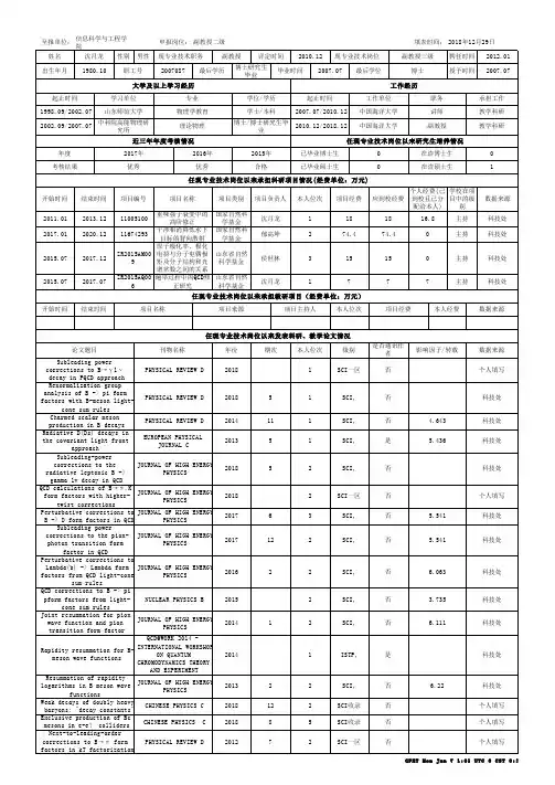
a rXi v :h e p -p h /9704448v 1 30 A p r 1997DESY 97-079IFT-96-29PM–97/04April 1997HDECAY:a Program for Higgs Boson Decaysin the Standard Model and its Supersymmetric ExtensionA.Djouadi 1,J.Kalinowski 2and M.Spira 31Laboratoire de Physique Math´e matique et Th´e orique,UPRES–A 5032,Universit´e de Montpellier II,F–34095Montpellier Cedex 5,France.2Deutsches Elektronen–Synchrotron,DESY,D–22603Hamburg,Germany,Institute of Theoretical Physics,Warsaw University,PL–00681Warsaw,Poland.3Theory Division,CERN,CH–1211,Geneva 23,Switzerland.Abstract We describe the Fortran code HDECAY †,which calculates the decay widths and the branching ratios of the Standard Model Higgs boson,and of the neutral and charged Higgs particles of the Minimal Supersymmetric extension of the Standard Model.The program is self-contained (with all subroutines included),easy to run,fast and calculates the decay widths and branching ratios according to the current theoretical knowledge.:f1IntroductionThe experimental observation of scalar Higgs particles is crucial for our present under-standing of the mechanism of electroweak symmetry breaking.Thus the search for Higgs bosons is one of the main entries in the LEP2agenda,and will be one of the major goals of future colliders such as the Large Hadron Collider LHC and the future Linear e+e−Collider LC.Once the Higgs boson is found,it will be of utmost importance to perform a detailed investigation of its fundamental properties,a crucial requirement to establish the Higgs mechanism as the basic way to generate the masses of the known particles.To this end,a very precise prediction of the production cross sections and of the branching ratios for the main decay channels is mandatory.In the Standard Model(SM),one doublet of scalarfields is needed for the electroweak symmetry breaking,leading to the existence of one neutral scalar particle H0[1].Once M H0isfixed,the profile of the Higgs boson is uniquely determined at tree level:the couplings to fermions and gauge bosons are set by their masses and all production cross sections,decay widths and branching ratios can be calculated unambiguously[2].Unfor-tunately,M H0is a free parameter.From the direct search at LEP1and LEP2we know that it should be larger than about71GeV[3].Triviality restricts the Higgs particle to be lighter than about1TeV;theoretical arguments based on Grand Unification at a scale ∼1016GeV suggest however,that the preferred mass region will be100GeV<∼M H0<∼200GeV;for a recent summary,see Ref.[4].In supersymmetric(SUSY)theories,the Higgs sector is extended to contain at least two isodoublets of scalarfields.In the Minimal Supersymmetric Standard Model(MSSM) this leads to the existence offive physical Higgs particles:two CP-even Higgs bosons h and H,one CP-odd or pseudoscalar Higgs boson A,and two charged Higgs particles H±[1].Besides the four masses,two additional parameters are needed:the ratio of the two vacuum expectation values,tgβ,and a mixing angleαin the CP-even sector. However,only two of these parameters are independent:choosing the pseudoscalar mass M A and tgβas inputs,the structure of the MSSM Higgs sector is entirely determined at lowest order.However,large SUSY radiative corrections[5]affect the Higgs masses and couplings,introducing new[soft SUSY-breaking]parameters in the Higgs sector. If in addition relatively light genuine supersymmetric particles are allowed,the whole set of SUSY parameters will be needed to describe the MSSM Higgs boson properties unambiguously.In this report we describe the program HDECAY1,which calculates the decay widths and branching ratios of Higgs bosons in the SM and the MSSM.It includes:•All decay channels that are kinematically allowed and which have branching ratios larger than10−4,y compris the loop mediated,the most important three body decay modes,and in the MSSM the cascade and the supersymmetric decay channels.•All relevant higher-order QCD corrections to the decays into quark pairs and to the quark loop mediated decays into gluons are incorporated in the most complete form[7].The largest part of the corrections to the heavy quark pair decay modes aremapped into running masses which have to be evaluated at the scale of the Higgs mass.The small leading electroweak corrections are also included.They become sizeable only in the large Higgs mass regime due to the enhanced self-interactions of the Higgs bosons.•Double off-shell decays of the CP-even Higgs bosons into massive gauge bosons which then decay into four massless fermions[8].These decays are important for masses close to M W or M Z.For larger masses,it is a sufficient approximation to switch offthese decays[which are CPU time consuming]and to allow for one on-shell gauge boson only.•All important below-threshold[three-body]decays:with off-shell heavy top quarks H0,H,A→t¯t∗→t¯bW−and H+→t∗¯b→b¯bW+;with one off-shell gauge boson H→W±∗H∓,H→Z∗A,A→Z∗h and H±→W±∗A,W±∗h;as well as the decays of H with one off-shell Higgs boson H→hh∗,AA∗.These three body decays can be rather important,especially in the MSSM[9](see also[10]).•In the MSSM,the complete radiative corrections in the effective potential approach with full mixing in the stop and sbottom sectors;it uses the renormalization group improved values of the Higgs masses and couplings,and the relevant leading next-to-leading-order corrections are also implemented[11].•In the MSSM,all the decays into SUSY particles when they are kinematically al-lowed.The decays into charginos and neutralinos are included in the most general case,and the decays to sleptons and squark pairs with sfermion mixing in the third generation sector[12].•In the MSSM,all SUSY particles are included in the loop mediatedγγand gg decay channels:charged Higgs bosons,chargino,slepton and squark[including mixing] loops in h,H→γγdecays,chargino loops in A→γγand squark loops in h,H→gg.In the gluonic decay modes the large QCD corrections for quark[13,14]and squark loops[15]are also included.The basic input parameters,fermion and gauge boson masses and their total widths, coupling constants and in the MSSM,soft SUSY-breaking parameters can be chosen from an inputfile.In thisfile severalflags allow to switch on/offor change some options[e.g. choose a particular Higgs boson,include/exclude the multi-body or SUSY decays,or include/exclude specific higher-order QCD corrections].The results for the many decay branching ratios and the total decay widths are written into several outputfiles with headers indicating the processes and giving the input parameters.The program is written in FORTRAN and has been tested on several machines:VAX stations under the operating system VMS and work stations running under UNIX.All the3necessary subroutines[e.g.for integration]are included.The program is lengthy[more than5000FORTRAN lines]but rather fast,especially if some options[as decays into double off-shell gauge bosons]are switched off.The rest of this report is organized as follows.In the next section we discuss the physical decay processes included in the program.We describe the parameters of the inputfile in Section3.In Section4,we present examples of outputfiles.Some comments and conclusions are given in Section5.2Decay Modes2.1Standard Modela)Decays to quarks and leptonsThe Higgs boson partial width for decays to massless quarks,directly coupled to the SM Higgs particle,is calculated including the O(α3s)QCD radiative corrections[16,17] in them Q(M H)and the strong coupling constantαs(M H)both defined at the scale of the Higgs boson mass.The quark masses can be neglected in the phase space and in the matrix element except for decays in the threshold region,where the next-to-leading-order QCD corrections are given in terms of the quark pole mass M Q[16].The relation between the perturbative pole quark mass(M Q)and the running m Q)at the scale of the pole mass can be expressed as[18]1+4π+K Q αs(M Q)MS massm Q(M Q)are adopted as starting points,because these are directly determined from QCD spectral sum rules[19]for the b and c quarks.Theflag NNLO(I)determines whether(I=1)the input running mass is related to the pole mass according to the eq.(1) or(I=0)using the simplified version with the K Q term neglected[in this case we denotethe pole mass by M pt2Q ].The input pole mass values and corresponding running massesare presented in Table1.The evolution from M Q upwards to a renormalization scaleµis given bym Q(M Q)c[αs(µ)/π]Q M pt2Q1.41GeV4.62GeV175.0GeVMS mass and the two different definitions of the pole masses.The strong coupling has been chosen asαs(M Z)=0.118and the bottom and charm mass values are taken from Ref.[19].with[20]c(x)= 99[1+0.895x+1.371x2]for M s<µ<M cc(x)= 2525[1+1.014x+1.389x2]for M c<µ<M bc(x)= 2323[1+1.175x+1.501x2]for M b<µ<M tc(x)= 77[1+1.398x+1.793x2]for M t<µFor the charm quark mass the evolution is determined by eq.(2)up to the scaleµ=M b, while for scales above the bottom mass the evolution must be restarted at M Q=M b. The values of the running b,c masses at the scaleµ=100GeV,characteristic for theHiggs mass,are typically35%(60%)smaller than the bottom(charm)pole masses M pt2b (M pt2).cThe program HDECAY includes the full massive NLO corrections close to the thresh-olds as well as the massless O(α3s)corrections far above the thresholds.The transition between both regions is provided by a linear interpolation as shown in Fig.1.Thus the result is optimized for the description of the mass effects in the threshold region and for the renormalization group improved large Higgs mass regime.The electroweak corrections to heavy quark and lepton decays in the intermediate Higgs mass range are small[21]and could thus be neglected,but the bulk of the effect [22]is included in the program.For large Higgs masses the electroweak corrections due to the enhanced self-coupling of the Higgs bosons are included,which however turn out to be small[23].In the case of t¯t decays of the Standard Higgs boson,the O(αs)QCD corrections are included according to[16].Below-threshold(three-body)decays H→t¯t∗→t¯bW−into off-shell top quarks may be sizeable[9]and thus are implemented.5Γ(H → bb) [MeV ]_M b = 4.62 GeV NLO massiveNNNLO (RG)M H [GeV ]8102030507010010-210-1110Figure 1:Interpolation between the full massive NLO expression (dashed line)for the b ¯b decay width of the Standard Higgs boson and the renormalization group improved NNNLO result (dotted line).The interpolated curve is presented by the full line.b)Decays to gluonsThe decay of the Higgs boson to gluons is mediated by heavy quark loops in the Standard Model;the partial decay width in lowest order is given in [24].QCD radiative corrections [13,14]are built up by the exchange of virtual gluons,gluon radiation from the internal quark loop and the splitting of a gluon into unresolved two gluons or a quark-antiquark pair.The radiative corrections are very large,nearly doubling the partial width.Since b quarks,and eventually c quarks,can in principle be tagged experimentally,it is physically meaningful to include gluon splitting g ∗→b c )in H →gg ∗→gb c )decays to the inclusive decay probabilities Γ(H →b ¯b +...)etc.[7].Separating this contribution generates large logarithms,which can be effectively absorbed by defining the number of active flavors in the gluonic decay mode in the input file of HDECAY by specifying the NF-GG parameter.The contributions of the subtracted flavors will automatically be added to the corresponding heavy quark decay modes.c)Decays to γγand ZγThe decay of the Higgs boson to two photons and to a photon and a Z boson,medi-ated by W and heavy fermion loops,are implemented according to [25].QCD radiative corrections are rather small [13,26]and thus neglected in the program.6d)Decays to W W/ZZ bosonsAbove the W W and ZZ decay thresholds the partial decay widths into pairs of on-shell massive gauge bosons are given in[27].Electroweak corrections are small in the intermediate mass range[28]and thus neglected in the program HDECAY.Higher order corrections due to the self-couplings of the Higgs particles are sizeable[29]for M H>∼400 GeV and are taken into account.Below the W W/ZZ threshold,the decay modes into off-shell gauge bosons are im-portant.With the input parameter ON-SH-WZ=1the program includes decays with one on-shell and one off-shell gauge boson[30],while for ON-SH-WZ=0decays with both off-shell are also calculated[8].The branching ratios for the latter reach the percent level for Higgs masses above about100(110)GeV for both W(Z)boson pairs off-shell.For higher masses,it is sufficient to allow for one off-shell gauge boson only,especially because the two virtual gauge boson option is CPU time consuming.2.2The Minimal Supersymmetric Standard ModelThe MSSM Higgs sector is implemented in HDECAY including the complete radiative corrections due to top/bottom quark and squark loops within the effective potential ap-proach.Next-to-leading order QCD corrections and the full mixing in the stop and sbottom sectors are incorporated.The Higgs boson mass spectrum,the mixing angles and Higgs boson couplings are calculated using the approximate formulae of M.Carena, M.Quiros and C.E.M.Wagner[11].The basic parameters describing the effective Higgs potential at higher orders are specified in the inputfile.The formulae for the decay widths at tree-level have been derived in Ref.[31].a)Decays to quarks and leptonsThe calculation of the partial decay widths of scalar neutral Higgs bosons h and H to fermions in the MSSM is performed using the same approximations and options as in the Standard Model case with properly modified Higgs boson couplings.For massless quarks the QCD corrections for scalar,pseudoscalar and charged Higgs boson decays are implemented analogously to the SM case[16,17],i.e.the Yukawa and QCD couplings are evaluated at the scale of the Higgs boson mass.In the threshold regions mass effects play a significant role,in particular for the pseu-doscalar Higgs boson,which has an S-wave behavior∝βas compared with the P–wave suppression∝β3for CP-even Higgs bosons[β=(1−4m2f/M2Φ)1/2is the velocity of the decay fermions].The QCD corrections to the partial decay width of the CP-odd Higgs boson A into heavy quark pairs are taken from Ref.[16],and for the charged Higgs par-ticles from Ref.[32].The transition from the threshold region,involving mass effects, to the renormalization group improved large Higgs mass regime is provided by a smooth linear interpolation analogous to the SM case.7Below the t¯t threshold,decays of the neutral Higgs bosons into off-shell top quarks are sizeable,thus modifying the profile of the Higgs particles significantly.Off-shell pseu-doscalar branching ratios reach a level of a few percent for masses above about300GeV for small tgβvalues.Similarly,below the t¯b threshold,off-shell decays H+→t∗¯b→b¯bW+ are important,reaching the percent level for charged Higgs boson masses above about100 GeV for small tgβvalues.These decays are incorporated according to the expressions from Ref.[9].b)Decays to gluonsSince the b quark couplings to the Higgs bosons may be strongly enhanced and the t quark couplings suppressed in the MSSM,b loops can contribute significantly to the Higgs-gg couplings so that the approximation M2Q≫M2H cannot be applied any more for MΦ<∼150GeV,where this decay mode is important.Nevertheless,it turns out a posteriori that this is an excellent approximation for the QCD corrections in the range, where these decay modes are relevant.The LO width for h,H→gg is generated by quark and squark loops with the latter contributing significantly for Higgs masses below about 400GeV[15].The partial decay widths are calculated according to Ref.[13,14].The bottom and charmfinal states from gluon splitting can be added to the corresponding b¯b and c¯c decay modes,as in the SM case,by defining NF-GG=3in the inputfile.c)Decays intoγγand ZγThe decays of the neutral Higgs bosons to two photons and a photon plus a Z boson are mediated by W and heavy fermion loops,as in the Standard Model,and in addition by charged Higgs,sfermion and chargino loops;the partial decay widths are calculated according to Ref.[13].QCD corrections to the quark and squark loop contributions are small[13,26]and thus neglected in the program.d)Decays to W W/ZZ gauge bosonsThe partial widths of the CP-even neutral MSSM Higgs bosons into W and Z boson pairs are obtained from the SM Higgs decay widths by rescaling with the corresponding MSSM couplings.They are strongly suppressed[due to kinematics in the case of h and reduced couplings for the heavy H],thus not playing a dominant role as in the SM case.e)Decays to Higgs boson pairsThe heavy CP-even Higgs particle can decay into a pair of light scalars as well to a pair of pseudoscalar Higgs bosons,H→hh and H→AA.While the former is the dominant decay mode of H in the mass range2M h<M H<2m t for small values of tgβ,the latter mode occurs only in a marginal area of the MSSM parameter space.For large values of tgβ,these decays occur only if M A∼M h<∼M H/2,corresponding to the lower end of the heavy Higgs mass range,and have branching ratios of50%each.Since the Hb¯b Yukawa coupling is strongly enhanced for large tgβ,below threshold decays H→hh∗,AA∗with A,h→b¯b are included[9].The lightest CP-even Higgs particle h can also decay into8pseudoscalar Higgs pairs for values tgβ∼1and M h<50GeV;however this area of the parameter space is already ruled out by present data[3].f)Decays to W/Z and Higgs bosonsThe Higgs bosons can also decay into a gauge boson and a lighter Higgs boson.The branching ratios for the two body decays A→hZ and H+→W+h may be sizeable in specific regions of the MSSM parameter space[small values of tgβand below the tt/tb thresholds for neutral/charged Higgs bosons].The expressions of the decay widths are given in e.g.Ref.[9].Below-threshold decays into a Higgs particle and an off-shell gauge boson turned out to be rather important for the heavy Higgs bosons of the MSSM.Off-shell A→hZ∗decays are important for the pseudoscalar Higgs boson for masses above about130GeV for small tgβ.The decay modes H±→hW∗,AW∗reach branching ratios of several tens of percent and lead to a significant reduction of the dominant branching ratio intoτνfinal states to a level of60%to70%for small tgβ.In addition,three-body H→AZ∗and H→H+W−∗,which are kinematically forbidden at the two-body level,can be sizeable for small M A values.The partial decay widths for these three-body decays are calculated according to the formulae given in Ref.[9].g)Decays to charginos and neutralinosThe lightest charginos and neutralinos are expected to have masses of the order of the Z boson mass.The heavy CP-even,CP-odd and charged Higgs bosons of the MSSM can therefore decay into these states[31].Present experimental bounds on the SUSY particle masses,do not allow decays for SUSY decay modes of the lightest CP-even Higgs boson h,except maybe for the decays into a pair of the lightest neutralinos.These decays,the partial widths of which can be found in Ref.[12],are included in the program.The masses of charginos and neutralinos as well as their couplings to the Higgs bosons depend on three extra parameters[in addition to those describing the Higgs sector at the tree-level]:the Higgs-Higgsino mass parameterµ[which also enters the radiative correc-tions in the Higgs sector],the Bino and Wino mass parameters M1and M2.Assuming a common gaugino mass at the unification scale,the parameter M1is related to M2by the GUT relation M1=5lead to very large decay widths.The sfermions masses and couplings to Higgs bosons will depend on three extra pa-rameters[in addition to tgβand M A]for each generation:the left-and right-handedsoft SUSY-breaking mass parameters M˜f L and M˜f R,the Higgs mass parameterµandthe trilinear coupling A f.The trilinear couplings are important only in the case of the third generation sfermions,and only A t,A b and Aτneed to be introduced.The latter couplings[at least A t and A b]also contribute to the radiative corrections to the Higgs sector.For the SUSY breaking scalar masses,we assumed degeneracy in thefirst and second generation and treated the third generation separately2.While the masses of the left-and right-handed1st/2nd generation sfermions correspond to the physical sfermion masses,in the third generation mixing between thesefields needs to be included to obtain the physical eigenstates[35].The masses of the sfermions,as well as their couplings to Higgs bosons,including the mixing in the generation are calculated in the subroutine SFERMION.The decay widths are calculated in the main subroutine using the formulae given in Ref.[12].The QCD corrections to squark decays[in particular stop and sbottom decays]have been calculated in Ref.[37]but are not yet implemented in the program.3How to Run HDECAY:Input FileThe HDECAY program is self-contained with all necessary subroutines included.In addition to the source code of the program HDECAY,an inputfile,defined as unit98, is needed from which the program reads the input parameters.The name of this input file can be specified in thefirst OPEN statement of HDECAY.It should be noted that the input numbers must not start before the equality signs in each corresponding line. The inputfile contains the following parameters[all non-integer parameters are in double precision and the mass parameters as well as the decay widths and the trilinear couplings are in GeV]:HIGGS:ratio of the vacuum expectation values in the MSSM,tgβ,the second basic input of the model;the program is suitable only for values tgβ>∼1.:end value of the Higgs mass in GeVNMA:strong coupling constant at the scale M Z:αS(M Z)MSBAR(1)MS mass of the strange quark at the scale Q=1GeVMC:bottom quark pole massMT:τlepton massMMUON:inverse QED coupling constant:α−1(0)GF:total decay width of the W bosonGAMZ:Z boson massMW:CKM parameter V usVCB:ratio of the CKM parameters V ub/V cb.MU:SUSY breaking gaugino mass parameter M2MSL1:SUSY breaking mass parameter for1st/2nd generation right-handed charged sleptons,M˜eRMSQ1:SUSY breaking mass parameter for1st/2nd generation right-handed down-type squarks,M˜d RMSL:SUSY breaking mass parameter for3rd generation right-handed sleptons,M˜τR MSQ:SUSY breaking mass parameter for right-handed stops,M˜tRMDR:SUSY breaking trilinear coupling forτsleptons,AτAU:SUSY breaking trilinear coupling for sbottoms,A bNNLO(M)MS masses=1:use O(α2s)formula for the quark pole masses→:integer=0:include three-body decays with off-shell tops,Higgs and gauge bosons=1:exclude three-body decays with off-shell tops,Higgs and gauge bosonsON-SH-WZ:integer=0:calculate:integer=0:include decays into and loops of supersymmetric particles=1:exclude decays into and loops of supersymmetric particlesINDIDECintegernumber of lightflavors included in the decaysΦ→gg∗→gq¯q(NF-GG=3,4or5).12The current values of the SM parameters[fermion masses,gauge boson masses and total widths,coupling constants,CKM angles]are given in Tab.2,where an example of the inputfile is displayed.The entire Higgs sector of the MSSM isfixed once the parameterstgβ,M A,µ,M2,the masses M˜L L ,M˜E R,M˜U L,M˜U R,M˜D Rand the trilinear couplings Aτ,A tand A b are specified.Some examples for these values are shown in Tab.2.4Results of Test Run:Output FilesThe output is written to severalfiles.Only the outputfiles of the chosen HIGGS bo-son(s)are printed,and they contain all decay branching ratios and the total decay width, except for the decays to SUSY particles[if OFF-SUSY=0]where only the sums of the branching ratios into charginos,neutralinos,sleptons and squarks are printed,if theflag INDIDEC=0;only for INDIDEC=1all individual branching ratios are printed in addi-tional outputfiles.For convenience,an outputfile br.input is printed in which the input parameters are given.Below we will describe the outputfiles in the SM and the MSSM [also with the option for SUSY decays switched on]and list all the decay channels which we have considered for the various Higgs bosons.4.1Standard Model Higgs bosonFor the SM Higgs boson,in addition to thefile br.input for the input parameters,two outputfiles are printed in which the total decay width and the following11branching ratios are given[notice that we have put the decays into fermions and gauge bosons into two differentfiles]br.sm1:M H0,BR(b¯b),BR(τ+τ−),BR(µ+µ−),BR(s¯s),BR(c¯c),BR(t¯t) br.sm2:M H0,BR(gg),BR(γγ),BR(γZ),BR(W W),BR(ZZ),Γtot H0For the example of inputfile shown in Tab.2,one obtains the two outputs given in Tab.3. The various branching ratios and the total decay width are shown in Fig.2.4.2MSSM without SUSY decaysAs discussed earlier,the two basic inputs of the program for the MSSM Higgs sector are tgβand M A.Once these parameters arefixed,all the other Higgs masses and couplings are determined at tree-level.However,subleading effects due to squark mixing[mainly the parameters A t,b andµ]will alter these values.For the lightest MSSM Higgs boson hHIGGS=0TGBET= 1.5D0MABEG=100.D0MAEND=500.D0NMA=5ALS(MZ)=0.118D0MSBAR(1)=0.190D0MC= 1.42D0MB= 4.62D0MT=175.D0MTAU= 1.7771D0MMUON=0.105658389D01/ALPHA=137.0359895D0GF= 1.16639D-5GAMW= 2.080D0GAMZ= 2.490D0MZ=91.187D0MW=80.33D0VUS=0.2205D0VCB=0.04D0VUB/VCB=0.08D0MU=300.D0M2=200.D0MSL1=500.D0MER1=500.D0MQL1=500.D0MUR1=500.D0MDR1=500.D0MSL=500.D0MER=500.D0MSQ=500.D0MUR=500.D0MDR=500.D0AL=1500.D0AU=1500.D0AD=1500.D0NNLO(M)=0ON-SHELL=0ON-SH-WZ=0IPOLE=0OFF-SUSY=1INDIDEC=0NF-GG=5Table2:Example of the inputfile.14Γ(H) [GeV ]M H [GeV ]50100200500100010-310-210-1110102BR(H)bb _τ+τ−cc _ggWW ZZtt-γγZ γM H [GeV ]50100200500100010-310-210-11Figure 2:Total decay width Γ(H )in GeV and the main branching ratios BR (H )of the Standard Model Higgs decay channels,using the inputs of Tab.2.15MHSM BB TAU TAU MU MU SS CC TT___________________________________________________________________________100.0000.81190.7926E-010.2752E-030.6048E-030.3698E-010. 200.0000.2596E-020.2884E-030.1000E-050.1928E-050.1177E-030. 300.0000.6082E-030.7274E-040.2521E-060.4513E-060.2754E-040.5293E-04 400.0000.2283E-030.2869E-040.9940E-070.1694E-060.1033E-040.1376 500.0000.1183E-030.1542E-040.5342E-070.8772E-070.5347E-050.1936MHSM GG GAM GAM Z GAM WW ZZ WIDTH___________________________________________________________________________100.0000.5807E-010.1532E-020.4654E-040.1025E-010.1046E-020.2598E-02 200.0000.8219E-030.5241E-040.1753E-030.73500.2609 1.428 300.0000.5674E-030.1289E-040.5670E-040.69130.30738.510 400.0000.7532E-030.3192E-050.1935E-040.58720.274128.89 500.0000.5476E-030.4897E-060.7666E-050.54500.260767.53 Table3:The two outputfiles in the SM with the inputs of Tab.2.For the heavy CP-even MSSM Higgs boson H,there are less possibilities than for the H bo-son:due to CP-invariance,the pseudoscalar A does not couple to gauge and Higgs boson pairs.The10decay channels are printed in the outputfiles as followsbr.a1:M A,BR(b¯b),BR(τ+τ−),BR(µ+µ−),BR(s¯s),BR(c¯c),BR(t¯t) br.a2:M A,BR(gg),BR(γγ),BR(γZ),BR(hZ),Γtot AFor the charged MSSM Higgs bosons H±。