multipath introduction
- 格式:doc
- 大小:41.50 KB
- 文档页数:2
IBM System Storage SAN Volume ControllerIBM Storwize V7000Information Center ErrataVersion 6.3.0April 27, 20121Contents Introduction (4)Who should use this guide (4)Last Update (4)Change History (4)iSCSI Limits (5)iSCSI Limits with Multiple I/O Groups (5)Definition of terms (5)Limits that take effect when using iSCSI (6)Single I/O Group Configurations (6)iSCSI host connectivity only (6)Mixed iSCSI and Fibre Channel host connectivity (6)Multiple I/O Group Config (7)Symptoms of exceeding the limits (7)Configuring the HP 3PAR F-Class and T-Class Storage Systems (8)Minimum Supported STORWIZE V7000 Version (8)Configuring the HP 3PAR Storage System (8)Supported models of HP 3PAR Storage Systems (8)Support firmware levels of HP 3PAR storage arrays (8)Concurrent maintenance on HP 3PAR storage arrays (8)HP 3PAR user interfaces (8)HP 3PAR Management Console (9)HP 3PAR Command Line Interface (CLI) (9)Logical units and target ports on HP 3PAR storage arrays (9)LUNs (9)LUN IDs (9)LUN creation and deletion (10)LUN Presentation (10)Special LUNs (10)LU access model (11)LU grouping (11)LU preferred access port (11)Detecting Ownership (11)Switch zoning limitations for HP 3PAR storage arrays (11)Fabric zoning (11)Target port sharing (11)Controller splitting (12)Configuration settings for HP 3PAR storage array (12)Logical unit options and settings for HP 3PAR storage array (12)Creation of CPG (12)Set up of Ports (13)Setup of Host (14)LUN creation (15)Host options and settings for HP 3PAR storage array (16)2Quorum disks on HP 3PAR storage arrays (16)Clearing SCSI reservations and registrations (17)Copy functions for HP 3PAR storage array (17)Thin Provisioning for HP 3PAR storage array (17)Recommended Settings for Linux Hosts (18)Multipath settings for specific Linux distributions and Releases (19)Udev Rules SCSI Command Timeout Changes (21)Editing the udev rules file (22)3IntroductionThis guide provides errata information that pertains to release 6.3.0 of the IBM System Storage SAN Volume Controller Information Center and the IBM Storwize V7000 Information Center.Who should use this guideThis errata should be used by anyone using iSCSI as a method to connect hosts, Connecting Linux hosts using Fibre Channel or when connecting HP 3PAR Storage to IBM System Storage SAN Volume Controller or IBM Storwize V7000 .Last UpdateThis document was last updated: April 27, 2012.Change HistoryThe following revisions have been made to this document:Revision Date Sections ModifiedNov 18, 2011 New publicationApr 27 2012 Linux Host SettingsTable 1: Change History4iSCSI LimitsiSCSI Limits with Multiple I/O GroupsThe information is in addition to, and a simplification of, the information provided in the Session Limits pages at the following links:/infocenter/StorwizeV7000/ic/index.jsp?topic=/com.ibm.storage.Storwize V7000.console.doc/StorwizeV7000_iscsisessionlimits.html/infocenter/storwize/ic/topic/com.ibm.storwize.v7000.doc/S torwize V7000_iscsisessionlimits.htmlDefinition of termsFor the purposes of this document the following definitions are used:IQN:an iSCSI qualified name – each iSCSI target or initiator has an IQN. The IQN should be unique within the network. Recommended values are of the formiqn.<date>.<reverse domain name>:<hostname>.<unique id> e.g. iqn.03-.ibm.hursley:host1.1initiator: an IQN that is used by a host to connect to an iSCSI targettarget: an IQN on an STORWIZE V7000 or V7000 node that is the target for an iSCSI logintarget portal: an IP address that can be used to access a target IQN. This can be either an IPv4 or an IPv6 address.5Limits that take effect when using iSCSISingle I/O Group ConfigurationsiSCSI host connectivity only1 target IQN per node2 iSCSI target portals (1xIPv4 and 1xIPv6) per network interface on a node4 sessions per initiator for each target IQN256 defined iSCSI host object IQNs512 host iSCSI sessions per I/O group **256 host iSCSI sessions per node (this is to allow the hosts to reconnect in the event of a failover)** e.g. if a single initiator logs in 3 times to a single target count this as 3. If a singleinitiator logs in to 2 targets via 3 target portals each count this as 6.Only the 256 defined iSCSI IQN limit is enforced by the GUI or CLI commands. Mixed iSCSI and Fibre Channel host connectivity512 total sessions per I/O group where:1 defined FC host object port (WWPN) = 1 session1 defined iSCSI host object IQN = 1 session1 additional iSCSI session to a target = 1 sessionIf the total number of defined FC ports & iSCSI sessions in an I/O group exceeds 512, some of the hosts may not be able to reconnect to the STORWIZE V7000/V7000 targets in the event of a node IP failover. See above section for help on calculating the number of iSCSI sessions.6Multiple I/O Group ConfigIf a host object is defined in more than one I/O group then each of its host object port definitions is counted against the session limits for every I/O group it is a member of. This is true for both FC and iSCSI host objects. By default a host object created using the graphical user interface is created in all available I/O groups.Symptoms of exceeding the limits.The following list is not comprehensive. It is given to illustrate some of the common symptoms seen if the limits defined above are exceeded.. These symptoms could also indicate other types of problem with the iSCSI network.•The host reports a time out during the iSCSI login process•The host reports a time out when reconnecting to the target after a STORWIZE V7000/V7000 node IP failover has occurred.In both of the above cases no errors will be logged by the STORWIZE V7000/V7000 system.7Configuring the HP 3PAR F-Class and T-Class Storage SystemsMinimum Supported STORWIZE V7000 Version6.2.0.4Configuring the HP 3PAR Storage SystemThis portion of the document covers the necessary configuration for using an HP 3PAR Storage System with an IBM Storwize V7000 cluster.Supported models of HP 3PAR Storage SystemsThe HP 3PAR F-Class (Models 200 and 400) the HP 3PAR T-Class (Models 400 and 800) are supported for use with the IBM STORWIZE V7000. These systems will be referred to as HP 3PAR storage arrays. For the latest supported models please visit /support/docview.wss?uid=ssg1S1003907Support firmware levels of HP 3PAR storage arraysFirmware revision HP InForm Operating System 2.3.1 (MU4 or later maintenance level) is the supported level of firmware for use with IBM STORWIZE V7000. For support on later versions, consult /support/docview.wss?uid=ssg1S1003907 Concurrent maintenance on HP 3PAR storage arraysConcurrent Firmware upgrades (“online upgrades”) are supported as per HP procedures. HP 3PAR user interfacesUsers may configure an HP 3PAR storage array with the 3PAR Management Console or HP 3PAR Command Line Interface (CLI).8HP 3PAR Management ConsoleThe management console accesses the array via the IP address of the HP 3PAR storage array. All configuration and monitoring steps are intuitively available through this interface.HP 3PAR Command Line Interface (CLI)The CLI may be installed locally on a Windows or Linux host. The CLI is also available through SSH.Logical units and target ports on HP 3PAR storage arraysFor clarification, partitions in the HP 3PAR storage array are exported as Virtual Volumes with a Virtual Logical Unit Number (VLUN) either manually or automatically assigned to the partition.LUNsHP 3PAR storage arrays have highly developed thin provisioning capabilities. The HP 3PAR storage array has a maximum Virtual Volume size of 16TB. A partition Virtual Volume is referenced by the ID of the VLUN.HP 3PAR storage arrays can export up to 4096 LUNs to the STORWIZE V7000 Controller (STORWIZE V7000’s maximum limit). The largest Logical Unit size supported by STORWIZE V7000 under PTF 6.2.0.4 is 2TB, STORWIZE V7000 will not display or exceeded this capacity.LUN IDsHP 3PAR storage arrays will identify exported Logical Units throughSCSI Identification Descriptor type 3.The 64-bit IEEE Registered Identifier (NAA=5) for the Logical Unit is in the form;5-OUI-VSID .The 3PAR IEEE Company ID of 0020ACh, the rest is a vendor specific ID.9Example 50002AC000020C3A.LUN creation and deletionVirtual Volumes (VVs) and their corresponding Logical Units (VLUNs) are created, modified, or deleted through the provisioning option in the Management Console or through the CLI commands. VVs are formatted to all zeros upon creation.To create a VLUN, highlight the Provisioning Menu and select the Create Virtual Volume option. To modify, resize, or destroy a VLUN, select the appropriate Virtual Volume from the window, right click when the specific VLUN is highlighted.*** Note: Delete the mdisk on the STORWIZE V7000 Cluster before deleting the LUN on the HP 3PAR storage array.LUN PresentationVLUNs are exported through the HP 3PAR storage array’s available FC ports by the export options on Virtual Volumes. The Ports are designated at setup and configured separately as either Host or Target (Storage connection). Ports being identified by a node : slot : port representation.There are no constraints on which ports or hosts a logical unit may be addressable.To apply Export to a logical unit, highlight the specific Virtual Volume associated with the Logical Unit in the GUI and right click and select Export.Special LUNsThere are no special considerations to a Logical Unit numbering. LUN 0 may be exported where necessary.Target PortsA HP 3PAR storage array may contain dual and/or quad ported FC cards. Each WWPN is identified with the pattern 2N:SP:00:20:AC:MM:MM:MM where N is the node, S is the slot and P is the port number on the controller and N is the controller’s address. The MMMMMM represents the systems serial number.Port 2 in slot 1 of controller 0 would have the WWPN of 20:12:00:02:AC:00:0C:3A The last 4 digits of serial number 1303130 in hex (3130=0x0C3A).This system has a WWNN for all ports of 2F:F7:00:02:AC:00:0C:3A.10LU access modelAll controllers are Active/Active. In all conditions, it is recommended to multipath across FC controller cards to avoid an outage from controller failure. All HP 3PAR controllers are equal in priority so there is no benefit to using an exclusive set for a specific LU.LU groupingLU grouping does not apply to HP 3PAR storage arrays.LU preferred access portThere are no preferred access ports on the HP 3PAR storage arrays as all ports are Active/Active across all controllers.Detecting OwnershipDetecting Ownership does not apply to HP 3PAR storage arrays.Switch zoning limitations for HP 3PAR storage arraysThere are no zoning limitations for HP 3PAR storage arrays.Fabric zoningWhen zoning an HP 3PAR storage array to the STORWIZE V7000 backend ports, be sure there are multiple zones or multiple HP 3PAR storage array and STORWIZE V7000 ports per zone to enable multipathing.Target port sharingThe HP 3PAR storage array may support LUN masking to enable multiple servers to access separate LUNs through a common controller port. There are no issues with mixing workloads or server types in this setup.Host splitting11There are no issues with host splitting on an HP 3PAR storage array.Controller splittingHP 3PAR storage array LUNs that are mapped to the Storwize V7000 cluster cannot be mapped to other hosts. LUNs that are not presented to STORWIZE V7000 may be mapped to other hosts.Configuration settings for HP 3PAR storage arrayThe management console enables the intuitive setup of the HP 3PAR storage array LUNs and export to the Storwize V7000 cluster.Logical unit options and settings for HP 3PAR storage array From the HP 3PAR storage array Management Console the following dialog of options are involved in setting up of Logical Units.Creation of CPGThe set up of Common Provisioning Groups (CPGs). If Tiering is to be utilised, it should be noted it is not good practice to mix different performance LUNs in the same STORWIZE V7000 mdiskgrp.Action->Provisioning->Create CPG (Common Actions)12Set up of PortsShown is on a completed 8 node STORWIZE V7000 cluster.Each designated Host ports should be set to Mode; point.Connection Mode: HostConnection Type: PointSystem->Configure FC Port (Common Actions)13Setup of HostHost Persona should be: 6 – Generic Legacy.All STORWIZE V7000 ports need to be included. Actions->Hosts->Create Host (Common Actions)14LUN creationSize limitations: 256 MiB minimum2TB maximum (STORWIZE V7000 limit)Provisioning: Fully Provision from CPGThinly ProvisionedCPG: Choose provisioning group for new LUN, usually R1,R5,R6 or drive specific. Allocation Warning: Level at which warning is given, optional [%]Allocation Limit: Level at which TP allocation is stopped, optional [%] Grouping: For creating multiple sequential LUNs in a set [integer values, 1-999] Actions->Provisioning->Create Virtual Volumes (Common Actions)15Exporting LUNs to STORWIZE V7000Host selection: choose host definition created for STORWIZE V7000Actions->Provisioning->Virtual Volumes->Unexported (Select VV and right click)Host options and settings for HP 3PAR storage arrayThe host options required to present the HP 3PAR storage array to Storwize V7000 clusters is, “6 legacy controller”.Quorum disks on HP 3PAR storage arraysThe Storwize V7000 cluster selects disks that are presented by the HP 3PAR storage array as quorum disks. To maintain availability with the cluster, ideally each quorum disk should reside on a separate disk subsystem.16Clearing SCSI reservations and registrationsYou must not use the HP 3PAR storage array to clear SCSI reservations and registrations on volumes that are managed by Storwize V7000. The option is not available on the GUI.Note; the following CLI command should only be used under qualified supervision,“setvv –clrsv”.Copy functions for HP 3PAR storage arrayThe HP 3PARs copy/replicate/snapshot features are not supported under STORWIZEV7000.Thin Provisioning for HP 3PAR storage arrayThe HP 3PAR storage array provides extensive thin provisioning features. The use of these thin provisioned LUNs is supported by STORWIZE V7000.The user should take notice of any warning limits from the Array system, to maintain the integrity of the STORWIZE V7000 mdisks and mdiskgrps. An mdisk will go offline and take its mdiskgroup offline if the ultimate limits are exceeded. Restoration will involve provisioning the 3PAR Array LUN, then including the mdisk and restoring any slandered paths.17Recommended Settings for Linux HostsThe following details the recommended multipath ( DMMP ) settings and udev rules for the attachment of Linux hosts to SAN Volume Controller and Storwize V7000. The settings are recommended to ensure path recovery in failover scenarios and are valid for x-series, all Intel/AMD based servers and Power platforms.A host reboot is required after completing the following two stepsEditing the multipath settings in etc/multipath.confEditing the udev rules for SCSI command timeoutFor each Linux distribution and releases within a distribution please reference the default settings under [/usr/share/doc/device-mapper-multipath.*] for Red Hat and[/usr/share/doc/packages/multipath-tools] for Novell SuSE. Ensure that the entries added to multipath.conf match the format and syntax for the required Linux distribution. Only use the multipath.conf from your related distribution and release. Do not copy the multipath.conf file from one distribution or release to another.Note for some OS levels the "polling_interval" needs to be located under defaults instead of under device settings.If "polling_interval" is present in the device section, comment out "polling_interval" using a # keyExamplesUnder Device Section# polling_interval 30,Under Defaults Sectiondefaults {user_friendly_names yespolling_interval 30}18Multipath settings for specific Linux distributions and ReleasesEdit /etc/multipath.conf with the following parameters and confirm the changes using “multipathd -k"show config".RHEL61device {vendor "IBM"product "2145"path_grouping_policy group_by_priogetuid_callout "/lib/udev/scsi_id --whitelisted --device=/dev/%n"features "1 queue_if_no_path"prio aluapath_checker turfailback immediateno_path_retry "5"rr_min_io 1# polling_interval 30dev_loss_tmo 120}RHEL56device {vendor "IBM"product "2145"path_grouping_policy group_by_prioprio_callout "/sbin/mpath_prio_alua /dev/%n"path_checker turfailback immediateno_path_retry 5rr_min_io 1# polling_interval 30dev_loss_tmo 120}19RHEL57device {vendor "IBM"product "2145"path_grouping_policy group_by_prioprio_callout "/sbin/mpath_prio_alua /dev/%n" path_checker turfailback immediateno_path_retry 5rr_min_io 1dev_loss_tmo 120}SLES10SP4device {vendor "IBM"product "2145"path_grouping_policy "group_by_prio"features "1 queue_if_no_path"path_checker "tur"prio "alua"failback "immediate"no_path_retry "5"rr_min_io "1"# polling_interval 30dev_loss_tmo 120}SLES11SP1device {vendor "IBM"product "2145"path_grouping_policy group_by_prioprio aluafeatures "0"no_path_retry 5path_checker turrr_min_io 1failback immediate# polling_interval 30dev_loss_tmo 12020}SLES11SP2device {vendor "IBM"product "2145"path_grouping_policy "group_by_prio"prio "alua"path_checker "tur"failback "immediate"no_path_retry "5"rr_min_io 1dev_loss_tmo 120}Udev Rules SCSI Command Timeout ChangesSet the udev rules for SCSI command timeoutSet SCSI command timeout to 120sOS Level Default Required SettingRHEL61 30 120RHEL62 30 120RHEL56 60 120RHEL57 60 120SLES10SP4 60 120SLES11SP1 60 120SLES11SP2 30 12021Creating a udev rules fileCreate the following udev rule that increases the SCSI command timeout for SVC and V7000 block devicesudev rules filecat /etc/udev/rules.d/99-ibm-2145.rules# Set SCSI command timeout to 120s (default == 30 or 60) for IBM 2145 devices SUBSYSTEM=="block", ACTION=="add", ENV{ID_VENDOR}=="IBM",ENV{ID_MODEL}=="2145", RUN+="/bin/sh -c 'echo 120 >/sys/block/%k/device/timeout'"Reconfirm the settings following the system reboot.22。

multipath多路径原理Multipath多路径原理是计算机网络中常见的一种技术,它通过使用多个路由路径来传输数据,从而提高数据传输的可靠性和性能,在数据传输中起到了至关重要的作用。
下面我们将详细阐述Multipath 多路径原理。
一、多路径技术概述传统的网络中,每个网络设备只有一种传输路径,数据只能通过这条路径进行传输。
但是,在现代网络环境中,单一路径无法满足高负载和高可用性的需求。
多路径技术允许在不同的路径上重复传输数据,从而使得数据传输更加灵活和高效。
二、Multipath多路径原理Multipath多路径原理是一种基于动态路由的技术,它通过将数据流分成多个流,每个流负责在不同的路径上传输数据。
在传输过程中,数据被拆分成多个数据包,每个数据包被分发到不同的路径上,通过各种高级路由协议计算出最优路径进行传输,重新组合成完整的数据包,最终传输到另一端,从而提高数据传输的速度和可靠性。
当数据包被发送时,传输协议会通过一系列路由算法计算出最佳路径,这些算法涉及到多种因素,包括网络拥塞、路由器负载、网络拓扑、网络带宽等。
然后,数据包将沿着这条路径传输,不过如果这条路径发生了阻塞,传输协议会选择另一条路径来传输数据包,这就保证了数据的可靠性和高可用性。
三、Multipath多路径技术的优势1、提高了网络传输的可靠性。
当一个路径被阻塞时,传输协议可以动态地选择另一条可用路径来传输数据,避免了数据丢失和传输延迟的问题。
2、提高了网络传输的性能。
多路径技术允许同时使用多个路径传输数据,因此可以实现更高的传输带宽和更低的传输延迟,从而提高了网络传输的性能和吞吐量。
3、提高了网络的可扩展性。
多路径技术可以有效地对网络进行分流,避免网络过载和拥塞,提高了网络的可扩展性和可维护性。
四、Multipath多路径技术的应用1、负载均衡:多路径技术可以用于实现负载均衡,同时利用多个路径来分配网络负载,保证每个路径都得到充分利用,提高了网络的效率和可靠性。
一、什么是多路径普通的电脑主机都是一个硬盘挂接到一个总线上,这里是一对一的关系。
而到了有光纤组成的SAN环境,或者由iSCSI组成的IPSAN环境,由于主机和存储通过了光纤交换机或者多块网卡及IP来连接,这样的话,就构成了多对多的关系。
也就是说,主机到存储可以有多条路径可以选择。
主机到存储之间的IO由多条路径可以选择。
每个主机到所对应的存储可以经过几条不同的路径,如果是同时使用的话,I/O流量如何分配?其中一条路径坏掉了,如何处理?还有在操作系统的角度来看,每条路径,操作系统会认为是一个实际存在的物理盘,但实际上只是通向同一个物理盘的不同路径而已,这样是在使用的时候,就给用户带来了困惑。
多路径软件就是为了解决上面的问题应运而生的。
多路径的主要功能就是和存储设备一起配合实现如下功能:1.故障的切换和恢复2.IO流量的负载均衡3.磁盘的虚拟化由于多路径软件是需要和存储在一起配合使用的,不同的厂商基于不同的操作系统,都提供了不同的版本。
并且有的厂商,软件和硬件也不是一起卖的,如果要使用多路径软件的话,可能还需要向厂商购买license才行。
比如EMC公司基于linux下的多路径软件,就需要单独的购买license。
好在, RedHat和Suse的2.6的内核中都自带了免费的多路径软件包,并且可以免费使用,同时也是一个比较通用的包,可以支持大多数存储厂商的设备,即使是一些不是出名的厂商,通过对配置文件进行稍作修改,也是可以支持并运行的很好的。
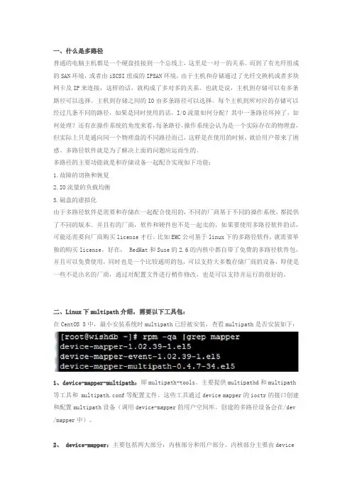
二、Linux下multipath介绍,需要以下工具包:在CentOS 5中,最小安装系统时multipath已经被安装,查看multipath是否安装如下:1、device-mapper-multipath:即multipath-tools。
主要提供multipathd和multipath 等工具和 multipath.conf等配置文件。
这些工具通过device mapper的ioctr的接口创建和配置multipath设备(调用device-mapper的用户空间库。

1/11/2007 4IQYKC ON FI DE NT IA LF O R A C C T O N T E C H N O L OG Y C O R P O R A TNET -AN100-R16215 Alton Parkway •P.O. Box 57013•Irvine, CA 92619-7013•Phone: 949-450-8700•Fax: 949-450-871008/06/04Networking Terms, Protocols, and Standards1/11/2007 4IQYKC ON FI D E NT IA L F O R A C C T O N T E C H N O L O G Y C O R P O R A T I O NBroadcom ®, the pulse logo, StrataXGS ®, and HiGig™ are trademarks of Broadcom Corporation and/or its subsidiaries in the United States and certain other countries. All other trademarks mentioned are the property of their respective owners.Broadcom CorporationP.O. Box 5701316215 Alton Parkway Irvine, CA 92619-7013© 2004 by Broadcom CorporationAll rights reserved Printed in the U.S.A.R EVISION H ISTORYRevision Date Change Description NET-AN100-R08/06/04Initial release.1/11/2007 4IQYKC ON FI DE NT IA LF O R A C C T O N T E C H N O L OG Y C O R P O R A T I O NApplication NoteNET08/06/04Broadcom CorporationDocument NET -AN100-RPage iiiT ABLE OF C ONTENTSIntroduction (1)Acronyms and Abbreviations..................................................................................................................1Standards and Protocols .. (3)IEEE 802.1d —Transparent Bridging......................................................................................................3IEEE 802.1q —Virtual LANs.. (4)IEEE 802.1p —Priority (4)IEEE 802.1s —Multiple Spanning Tree (5)IEEE 802.1w —Rapid Spanning Tree.....................................................................................................5IEEE 802.1x —Port-Based Authentication and Security. (5)IEEE 802.3x —Full-Duplex Flow Control.................................................................................................6IEEE 802.3ab —1000BASE-T. (6)IEEE 802.3ad —Link Aggregation..........................................................................................................7IEEE 803.2ae —10GBASE-X .................................................................................................................7IEEE 803.2ah —Ethernet in the First Mile. (7)High-Level Data Link Control..................................................................................................................7Internet Protocol.. (8)Internet Protocol Version 4 (8)IP Version 6.....................................................................................................................................8Transmission Control Protocol................................................................................................................9User Datagram Protocol . (9)Internet Control Message Protocol .......................................................................................................10Internet Group Management Protocol (10)Generic Attribute Registration Protocol (10)GARP VLAN Registration Protocol (10)Multiprotocol Label Switching ...............................................................................................................11Label Distribution Protocol....................................................................................................................11Constraints-Based Label Distribution Protocol.. (12)Border Gateway Protocol Version 4......................................................................................................12Open Shortest Path First ......................................................................................................................12Cisco Discovery Protocol......................................................................................................................12Link Layer Discovery Protocol ..............................................................................................................12Resource Reservation Protocol (13)1/11/2007 4IQYKC ON FI DE NT IA LF O R A C C T O N T E C H N O L OG Y C O R P O R A T I O NNET Application Note08/06/04Broadcom CorporationPage ivDocumentNET -AN100-RProtocol Applications (13)Transparent LAN Services (13)Virtual Private LAN Services Using MPLS (13)Virtual Private LAN Services Using Q-in-Q...........................................................................................15Hierarchal Transparent LAN Services (15)Differentiated Services (16)RFC-2547—BGP/MPLS VPNs..............................................................................................................16RFC-2697—Single-Rate Three-Color Marker.......................................................................................17RFC-2698—Two Rate Three-Color Marker. (17)RFC-3519—Mobile IP Traversal of NAT Devices .................................................................................17RFC-2890—Key and Sequence Number Extensions to GRE (17)Distance Vector Multicasting Routing Protocol (18)Protocol Independent Multicast.............................................................................................................18Protocol Independent Multicast-Sparse Mode.......................................................................................18Protocol Independent Multicast-Dense Mode........................................................................................19Protocol Independent Multicast-Source Specific Multicast.. (19)Routing Concepts (19)Equal Cost Multipath Routing (19)Weighted Cost Multipath Routing..........................................................................................................19MAC/PHY Interconnects .. (20)Media Independent Interface (20)Pin Descriptions (20)Reduced Media Independent Interface (22)Pin Descriptions (22)Serial Media Independent Interface (23)Pin Descriptions (24)Source-Synchronous Serial Media Independent Interface (25)Pin Descriptions .............................................................................................................................25Gigabit Media Independent Interface. (27)Pin Descriptions (27)Reduced Gigabit Media Independent Interface (29)Pin Descriptions (29)Serial Gigabit Media Independent Interface (31)Pin Descriptions (31)10-Bit Interface (32)1/11/2007 4IQYKC ON F I DE NT IA LF O R A C C T O N T E C H N O L OG Y C O R P O R A T I O NApplication NoteNET08/06/04Broadcom CorporationDocument NET -AN100-RPage vPin Descriptions.............................................................................................................................32Reduced 10-Bit Interface. (33)Pin Descriptions (33)10-Gigabit Media Independent Interface (35)Pin Descriptions (35)10-Gigabit Attachment Unit Interface (37)Pin Descriptions (37)HiGig—Broadcom 10-Gigabit Stacking Interface..................................................................................39HiGig+—Broadcom 12-Gigabit Stacking Interface.. (39)Media Technologies (39)100BASE-TX.........................................................................................................................................39100BASE-FX.........................................................................................................................................391000BASE-SX ......................................................................................................................................391000BASE-LX.......................................................................................................................................391000BASE-CX......................................................................................................................................401000BASE-T.. (40)ANSI 1000BASE-TX.............................................................................................................................40CX-4 (40)Gigabit Interface Converter (40)Small Form Factor Transceiver (41)SFF Pluggable Transceiver ..................................................................................................................41XENPAK .. (42)10-Gigabit SFF Pluggable.....................................................................................................................42Other Networking Terms (43)Asymmetric Digital Subscriber Line (43)Very High Data Rate Digital Subscriber Line (43)Protocol Header Formats (44)IPv4 (44)Version (44)Internet Header Length..................................................................................................................44Type of Service..............................................................................................................................44Total Length...................................................................................................................................45Identification...................................................................................................................................45Flags..............................................................................................................................................45Fragment Offset.. (45)1/11/2007 4IQYKC ON FI DE NT IA LF O R A C C T O N T E C H N O L OG Y C O R P O R A T I O NNET Application Note08/06/04Broadcom CorporationPage viDocumentNET -AN100-RTime-to-Live...................................................................................................................................45Protocol (45)Header Checksum..........................................................................................................................46Source Address (46)Destination Address.......................................................................................................................46Options...........................................................................................................................................46Data................................................................................................................................................46IPv6. (47)Version (47)Priority (47)Flow Label......................................................................................................................................47Payload Length..............................................................................................................................47Next Header.. (47)Hop Limit........................................................................................................................................47Source Address (47)Destination address........................................................................................................................47TCP. (48)Source Port (48)Destination Port..............................................................................................................................48Sequence Number . (48)Acknowledgment Number (48)Data Offset.....................................................................................................................................48Reserved........................................................................................................................................48Control Flags. (48)Window (49)Checksum (49)Urgent Pointer (49)Options...........................................................................................................................................49Data................................................................................................................................................49UDP. (49)Source Port ....................................................................................................................................49Destination Port..............................................................................................................................49Length............................................................................................................................................49Checksum ......................................................................................................................................50Data (50)1/11/2007 4IQYKC ON FI DE NT IA LF O R A C C T O N T E C H N O L OG Y C O R P O R A T I O NApplication NoteNET08/06/04Broadcom CorporationDocument NET -AN100-RPage viiMPLS (50)Label..............................................................................................................................................50EXP................................................................................................................................................50S ....................................................................................................................................................50TTL ................................................................................................................................................50ICMP.. (50)Type (50)Code..............................................................................................................................................50Checksum......................................................................................................................................51Identifier.. (51)Sequence Number.........................................................................................................................51Address Mask................................................................................................................................51IGMP.. (52)Version...........................................................................................................................................52Type.. (52)Max Response Time......................................................................................................................52Checksum.. (52)Group Address...............................................................................................................................52IGMP Version Membership Report Messages. (52)Type (53)Reserved .......................................................................................................................................53Checksum.. (53)Number of Group Records.............................................................................................................53Group Record.. (53)Group Record Type.......................................................................................................................53RSVP. (54)Version (54)Flags..............................................................................................................................................54Message Type. (54)RSVP Checksum...........................................................................................................................54Send TTL.......................................................................................................................................54RSVP Length (54)IEEE 802.1q (55)EtherType (55)1/11/2007 4IQYKC ON FI DE NT IA LF O R A C C T O N T E C H N O L OG Y C O R P O R A T I O NNET Application Note08/06/04Broadcom CorporationPage viiiDocumentNET -AN100-RPriority............................................................................................................................................55CFI..................................................................................................................................................55VID . (55)1/11/2007 4IQYKC ON FI DE NT IA LF O R A C C T O N T E C H N O L OG Y C O R P O R A T I O NApplication NoteNET08/06/04Broadcom CorporationDocument NET -AN100-RPage ixL IST OF F IGURESFigure 1: MPLS VPLS Example .......................................................................................................................14Figure 2: Q-in-Q VPLS Example ......................................................................................................................15Figure 3: MII Signal Connections .....................................................................................................................21Figure 4: RMII Signal Connections...................................................................................................................22Figure 5: SMII Signal Connections...................................................................................................................24Figure 6: S3MII Signal Connections.................................................................................................................26Figure 7: GMII Signal Connections...................................................................................................................28Figure 8: RGMII Signal Connections................................................................................................................30Figure 9: SGMII Signal Connections................................................................................................................31Figure 10: TBI Signal Connections...................................................................................................................32Figure 11: RTBI Signal Connections. (34)Figure 12: XGMII Signal Connections..............................................................................................................36Figure 13: XAUI Signal Connections................................................................................................................38Figure 14: Typical GBIC...................................................................................................................................40Figure 15: Typical SFF.....................................................................................................................................41Figure 16: Typical SFP.....................................................................................................................................41Figure 17: Typical XENPAK .. (42)Figure 18: Typical XFP (42)NET Application Note08/06/04NOITAROPROCYGOLONHCETNOTCCAROFLAITNEDIFNOCBroadcom CorporationPage x Document NET-AN100-R1/11/2007 4IQYK1/11/2007 4IQYKC ON FI DE NT IA LF O R A C C T O N T E C H N O L OG Y C O R P O R A T I O NBroadcom CorporationDocument NET -AN100-RPage xiL IST OF T ABLESTable 1: Acronyms and Abbreviations................................................................................................................1Table 2: Spanning Tree Port States...................................................................................................................3Table 3: Rapid Spanning Tree Port States (5)Table 4: PAUSE Timer Ranges..........................................................................................................................6Table 5: IP Services . (8)Table 6: Common TCP Port Numbers................................................................................................................9Table 7: MII Signal Definitions..........................................................................................................................20Table 8: RMII Signal Definitions.......................................................................................................................22Table 9: SMII Signal Definitions .. (24)Table 10: S3MII Signal Definitions ...................................................................................................................25Table 11: GMII Signal Definitions (27)Table 12: RGMII Signal Definitions ..................................................................................................................29Table 13: SGMII Signal Definitions...................................................................................................................31Table 14: TBI Signal Definitions.......................................................................................................................32Table 15: RTBI Signal Definitions (33)Table 16: XGMII Signal Definitions...................................................................................................................35Table 17: XAUI Signal Definitions . (37)Table 18: ADSL Downstream Speeds..............................................................................................................43Table 19: VDSL Downstream Speeds..............................................................................................................43Table 20: ICMP Type/Code Combinations. (51)OITAROPROCYGOLONHCETNOTCCAROFLAITNEDIFNOCBroadcom CorporationPage xii Document NET-AN100-R1/11/2007 4IQYK1/11/2007 4IQYKC ON FI DE NT IA LF O R A C C T O N T E C H N O L OG Y C O R P O R A T I O Broadcom CorporationDocument NET -AN100-RIntroductionPage 1I NTRODUCTIONThis document provides a high-level definition for several of the most commonly-used networking terms, protocols, and standards. The goal is to ensure that everyone has the same basic vocabulary foundation to promote better understanding during high-level feature discussions.This is not meant to be all encompassing networking terms glossary, but rather a targeted list of definitions that specifically apply to Broadcom’s current and future generation devices. Since Broadcom is continuously adding new features to their devices, this document will be updated periodically with pertinent information that pertains to the feature additions.A CRONYMS AND A BBREVIATIONSThe following tables list the acronyms and abbreviations within this document.Table 1: Acronyms and AbbreviationsAcronym/Abbreviation Description4D-PAM5Four-Dimensional/Pulse-Amplitude-ModulationADSL Asymmetric Digital Subscriber Line BGP Border Gateway Protocol BGP-4BGP version 4BPDU Bridge Protocol Data Units CBS Committed Burst Size CDP Cisco Discovery ProtocolCE Customer EdgeCFI Canonical Format Indicator CIR Committed Information RateCoS Class of ServiceCR-LDP Constraints-based Label Distribution ProtocolCVID Customer VLAN ID DDR Double-data RateDiffServ Differentiated Services DSL Digital Subscriber LineDSLAM Digital Subscriber Line Access MultiplexerDVMRP Distance Vector Multicasting Routing ProtocolEAPOL Extensible Authentication Protocol over LANEAP Extensible Authentication Protocol EBSExcess Burst SizeECMP Equal Cost Multipath EFMEthernet in the First Mile EPON Ethernet Passive Optical Network ETTB Ethernet to the Business ETTH Ethernet to the home ETTX Ethernet to the XFEC Forwarding Equivalence Class FCS Frame Check Sequence FFP Fast Filter Processor FIFOFirst-in First-outFTPFile Transfer ProtocolGARP Generic Attribute Registration Protocol GBIC Gigabit Interface Converter GMII Gigabit Media Independent Interface GREGeneric Routing EncapsulationGVRP GARP VLAN Registration Protocol HDLC High-Level Data Link Control HTLS Hierarchal Transparent LAN Services HTTPHyper Text Transfer Protocol ICMP Internet Control Message Protocol IETF Internet Engineering Task Force IGMP Internet Group Management Protocol IHL Internet Header Length IP Internet ProtocolIPv4Internet Protocol Version 4IPv6Internet Protocol Version 6ISN Initial Sequence Number LAN Local Area NetworkLACP Link Aggregation Control ProtocolAcronym/Abbreviation Description1/11/2007 4IQYKC ON FI DE NIA LF O R A C C T O N T E C H N O L OG Y C O R O R A T I O Broadcom CorporationPage 2IntroductionDocumentNET -AN100-RLDP Label Distribution Protocol LER Label Edge RouterLLDP Link Layer Discovery Protocol LSP Label-Switched Path LSR Label-Switched RouterMAC Media Access ControllerMII Media Independent Interface MLT-3Multi-Level Transmission-3MSA Multi-Source Agreement MSTP Multiple Spanning Tree Protocol MTU Multitenant UnitMPLS Multiprotocol Label Switching NAT Network Address Translation NEXT Near-End Cross-Talk NRZ Non-Return to ZeroNRZI Non-Return to Zero Inverted OSPF Open Shortest PathFirst PE Provider Edge PHY Physical layer devicePIM Protocol Independent MulticastPIM-DM Protocol Independent Multicast-Dense ModePIM-SM Protocol Independent Multicast-Sparse ModePIM-SSM Protocol Independent Multicast-Source Specific Multicast PIR Peak Information Rate POP3Post Office Protocol Version 3POTS Plain Old Telephone Service PPP Point-to-Point Protocol QoS Quality-of-ServiceRGMII Reduced Gigabit Media Independent InterfaceRIPv2Routing Information Protocol, Version 2RMII Reduced Media Independent InterfaceRP Rendezvous Point RPT Rendezvous Point Trees RSTP Rapid Spanning Tree ProtocolRSVP Resource Reservation ProtocolRTBI Reduced 10-Bit InterfaceS3MII Source-Synchronous Serial Media Independent Interface SFFSmall Form FactorAcronym/Abbreviation DescriptionSFP Small Form Factor Pluggable SGMII Serial Gigabit Media Independent InterfaceSMIISerial Media Independent InterfaceSMTP Simple Mail Transfer Protocol SNMPSimple Network Management Protocol SPT Shortest Path Tree SPVID Service Provider VLAN ID srTCMSingle-Rate Three-Color Marker SSM Source Specific MulticastSTP Spanning Tree Protocol TBI 10-Bit InterfaceTCP Transmission Control Protocol TLS Transparent LAN ServicesTLVType-Length-Value ToS Type of ServicetrTCM Two-Rate Three-Color Marker TTL Time-to-LiveUDP User Datagram Protocol UTPUnshielded Twisted PairVDSL Very high Data Rate Digital Subscriber LineVIDVLAN IdentifierVLAN Virtual Local Area NetworkWAN Wide Area Network VPLS Virtual Private LAN ServiceWCMPWeighted Cost MultipathXAUI 10-Gigabit Attachment Unit Interface XFP10-Gigabit Small Form Factor PluggableXGMII10-Gigabit Media Independent InterfaceAcronym/Abbreviation Description1/11/2007 4IQYKC ON FI DE NT IA LF O R A C C T O N T E C H N O L OG Y C O R P O R A T I O Broadcom CorporationDocument NET -AN100-RStandards and ProtocolsPage 3S TANDARDS AND P ROTOCOLSBecause there are so many different terms throughout the networking industry, it can be difficult to remember which are standards and which are protocols. This section identifies some of the most common of each.IEEE 802.1d —T RANSPARENT B RIDGING802.1d is the industry standard for the transparent bridge designed to ensure interoperability between bridge venders. One of the most important aspects of 802.1d is the Spanning Tree Protocol (STP). STP is a link management protocol that provides path redundancy while preventing loops in the network, a common problem introduced by Local Area Network (LAN) bridging.Only one active path can safely exist between to hosts. Multiple active paths between hosts are referred to as loops. These loops can confuse switches, resulting in various ill effects including duplicate packets and never-ending broadcasts.To provide path redundancy, STP defines a tree that spans all switches in an extended network. STP forces certain redundant data paths into a standby or blocked state. If one network segment in the STP becomes unreachable, or if STP costs change, the Spanning Tree algorithm reconfigures the Spanning Tree topology and reestablishes the link by activating the standby path.STP operation is transparent to end stations, which are unaware whether they are connected to a single LAN segment or a switched LAN of multiple segments. Spanning Tree enabled devices communicate to one another by exchanging Bridge Protocol Data Units (BPDUs).The way STP controls equipment ports is by setting them to one of five port states. The following table summarizes the capabilities of each state.All Broadcom switch devices support Spanning Tree by allowing the management software to set the port state. All devices also have some mechanism for detecting BPDUs and forwarding them to the management software.Table 2: Spanning Tree Port StatesPort State Receive BPDUs Transmit BPDUsLearn AddressesForward PacketsDisabled Blocking X Listening X X Learning X XXForwardingXXXX。

Recent Advances in Underwater Acoustic Communications & Networking水声通信与网络研究进展Abstract– The past three decades have seen a growing interest in underwater acousticcommunications. Continued research over the years has resulted in improved performance androbustness as compared to the initial communication systems. Research has expanded frompoint-to-point communications to include underwater networks as well. A series of review papers provide an excellent history of the development of the field until the end of the last decade. In this paper, we aim to provide an overview of the key developments, both theoretical and applied, in the field in thepast two decades. We also hope to provide an insight into some of the open problems and challenges facingresearchers in this field in the near future.抽象过去三十年来,在水声通信的兴趣与日俱增。

linux 存储多路径静默参数摘要:1.背景介绍2.Linux 存储多路径的概念3.静默参数的含义4.多路径静默参数的配置方法5.配置多路径静默参数的优点6.总结正文:1.背景介绍在Linux 系统中,存储设备通常通过多路径(multipath)技术来提高数据的可靠性和可访问性。
多路径技术允许系统同时访问多个物理存储设备,将它们作为一个逻辑设备来使用。
这种方式可以在某个存储设备出现故障时,自动切换到其他存储设备,从而保证数据的连续性和完整性。
2.Linux 存储多路径的概念Linux 中的多路径技术是通过multipath 模块来实现的。
multipath 模块可以在系统中创建一个虚拟的存储设备,它将多个物理存储设备关联起来,形成一个逻辑设备。
这个逻辑设备可以有多个入口点,即多路径。
当某个物理存储设备发生故障时,multipath 模块会将其从虚拟设备中移除,并将其他物理存储设备作为新的入口点加入虚拟设备,从而保证数据的可访问性。
3.静默参数的含义静默参数(silent parameters)是指在Linux 系统中,某些设备或模块在初始化时没有输出相关信息,但这些信息对于系统的正常运行是非常重要的。
静默参数通常在设备的配置文件中设置,如/etc/multipath/multipath.conf。
如果没有正确设置静默参数,可能会导致系统在启动时出现错误,甚至无法正常运行。
4.多路径静默参数的配置方法要在Linux 系统中配置多路径静默参数,需要编辑/etc/multipath/multipath.conf 文件。
在这个文件中,可以添加、修改或删除静默参数。
以下是一个配置多路径静默参数的示例:```# /etc/multipath/multipath.conf# 设置静默参数silent_aries = 3silent_param_check = 1silent_device_check = 1silent_mount_check = 1silent_module_check = 1silent_io_check = 1silent_udev_check = 1silent_hotplug_check = 1silent_firmware_check = 1silent_kernel_check = 1silent_builtin_check = 1silent_sbin_check = 1silent_sysfs_check = 1silent_block_check = 1silent_ Files_check = 1silent_dir_check = 1silent_socket_check = 1silent_module_exit_check = 1silent_module_load_check = 1silent_module_unload_check = 1silent_device_add_check = 1silent_device_del_check = 1silent_device_change_check = 1silent_path_check = 1silent_link_check = 1silent_init_check = 1silent_exit_check = 1silent_run_check = 1```在这个示例中,我们设置了silent_aries、silent_param_check、silent_device_check 等参数为1,表示启用这些静默参数的检查功能。
Doc. A/7418 June 2004ATSC Recommended Practice:Receiver Performance GuidelinesAdvanced Television Systems Committee1750 K Street, N.W.Suite 1200Washington, D.C. 20006The Advanced Television Systems Committee, Inc., is an international, non-profit organization developing voluntary standards for digital television. The ATSC member organizations represent the broadcast, broadcast equipment, motion picture, consumer electronics, computer, cable, satellite, and semiconductor industries. Specifically, ATSC is working to coordinate television standards among different communications media focusing on digital television, interactive systems, and broadband multimedia communications. ATSC is also developing digital television implementation strategies and presenting educational seminars on the ATSC standards.ATSC was formed in 1982 by the member organizations of the J oint Committee on InterSociety Coordination (J CIC): the Electronic Industries Association (EIA), the Institute of Electrical and Electronic Engineers (IEEE), the National Association of Broadcasters (NAB), the National Cable and Telecommunications Association (NCTA), and the Society of Motion Picture and Television Engineers (SMPTE). Currently, there are approximately 140 members representing the broadcast, broadcast equipment, motion picture, consumer electronics, computer, cable, satellite, and semiconductor industries.ATSC Digital TV Standards include digital high definition television (HDTV), standard definition television (SDTV), data broadcasting, multichannel surround-sound audio, and satellite direct-to-home broadcasting.Table of Contents1.SCOPE AND DOCUMENT STRUCTURE (8)1.1Foreword 81.2Scope 81.3Document Structure 8RMATIVE REFERENCES (9)3.SYSTEM OVERVIEW (9)3.1Objective 93.2System Block Diagrams 94.RECEIVER PERFORMANCE GUIDELINES (11)4.1Sensitivity 114.2Multi-Signal Overload 114.3Phase Noise 124.4Selectivity 124.4.1Co-Channel Rejection 124.4.2First Adjacent Channel Rejection 134.4.3Taboo Channel Rejection 134.4.3.1DTV Interference into DTV 144.4.3.2NTSC Interference into DTV 144.4.4Burst Noise Performance 144.5Multipath 154.5.1Introduction 154.5.2Field Ensembles 154.5.2.1Capture Location 154.5.2.2List of Recommended Field Ensembles 154.5.2.3Field Ensemble Characterization 164.5.2.4Data Format 174.5.2.5Recommended Physical Support for Field Ensemble Data Transfer 174.5.3Laboratory Ensembles 184.5.3.1Channel Impulse Response Range 184.5.3.1.1Typical Echo Range 184.5.3.1.2Single Static Echoes Amplitude / Equalizer Profile 184.5.3.2Single Dynamic Echoes 204.5.3.3Multiple Dynamic Echo Ensembles 214.5.3.4Dynamic Multipath in the Presence of Doppler Frequency Shift and Airplane Flutter234.6Antenna Interface 234.7Consumer Interface—Received Signal Quality Indicator 24ANNEX A:CAPTURE LABELS AND DESCRIPTIONS (25)ANNEX B:IMPULSE RESPONSE ANALYSIS (36)1.SCOPE (36)2.CHANNEL IMPULSE RESPONSE ANALYSIS (36)2.1Data Analysis Using Real Versus Complex Demodulators/Equalizers 362.2Channel Estimations Using 511 Pseudo-Random Sequence 362.3Frequency Doppler Estimate 392.3.1Comments on Doppler Analysis 392.3.2Methodology for Doppler Frequency Estimate 403.ANALYSIS OF RF CAPTURED DTV SIGNAL (41)3.1Captured Channel WAS-105/51/01 413.2Captured Channel WAS-032/39/011 (Indoor) 443.3Captured Cannel WAS-049/36/011 473.4Captured Channel WAS-034/48/01 553.5Captured Channel WAS-311/48/01 573.6Captured Channel WAS-114/27/011 603.7Captured Channel WAS-101/39/011 613.8Captured Channel NYC-216/56/01 623.9Captured Channel NYC-217/56/01 63 ANNEX C:EXAMPLE OF CHANNEL IMPULSE RESPONSE WITH LONG PRE AND POST-ECHO (64)1.SCOPE (64)1.1Far Pre-Echo 641.2Far Post-Echo 65 ANNEX D:ANALYSIS OF RECEIVED POWER FOR A SAMPLE RECEIVER (66)Index of Tables and FiguresTable 4.1 Co-Channel Rejection Thresholds 12 Table 4.2 First Adjacent Channel Thresholds 13 Table 4.3 Taboo Channel Rejection Thresholds for DTV Interference into DTV 14 Table 4.4 Taboo Channel Rejection Thresholds for NTSC Interference into DTV 14 Table 4.5 Field Ensemble Description 16 Table 4.6 ATSC Test Group R.1. Multiple Dynamic Echoes 20 Table 4.7 ATSC R.1 Ensembles 20 Table 4.8 ATSC Test Group R.2. Multiple Static and Dynamic Echoes 21 Table 4.9 ATSC R2.1 Ensembles 22 Table 4.10 ATSC R2.2 Ensembles 22 Table D.1 TV/DTV Received Power Analysis; Location: Hollywood, Fla. 67Figure 3.1 Overall block diagram of the digital terrestrial television broadcasting model. 10 Figure 3.2 Digital television receiver front-end subsystem block diagram. 11 Figure 4.3 Recommended target performance for a desired DTV signal in the presence of a single static echo of varying delay. 19 Figure A.1 RF capture spreadsheet. (Note: an electronic version of this Microsoft Excel document is available from ATSC.) 26 Figure B.1 Method of channel estimation using the PN511 pseudo-random number sequence in the 8-VSB field sync involves a cross correlation with three ideal PN511 sequences. 37 Figure B.2 Cross-correlation of an ideal 8-VSB PN511 sequence showing a single main path at zero microseconds. 37 Figure B.3 Channel estimation of an 8-VSB signal capture in the laboratory in the presence of a10 µs echo that is 6 dB lower in power than the main path. 38 Figure B.4 Power compensation function required to obtain the actual echo power from channel estimations using the 8-VSB PN511 sequence. 39 Figure B.5 Peak echo power as a function of echo delay observed for the duration of the RF capture at site WAS-105/51/01. 41 Figure B.6 Power of the main path in addition to the greatest “echoes” shows considerable variation over the duration of the RF capture for site WAS-105/51/01. 42 Figure B.7 Total power of the main path and ±3 “echoes” about the main path illustrating the power is constant even though the main path is dynamic. 43 Figure B.8 Peak echo power as a function of echo delay observed for the duration of the RF capture at indoor site WAS-32/39/01. 44Figure B.9 The 11 µs echo magnitude at the beginning of the capture at indoor site WAS-32/39/01. Doppler frequency is 75 Hz. 45Figure B.10 The 11 µs echo magnitude 6.9 seconds into the capture at indoor site WAS-32/39/01. Doppler frequency is 17 Hz. 46Figure B.11 Peak echo power as a function of echo delay observed for the duration of the RF capture at indoor site WAS-49/36/01. The evenly spaced echoes peaked at ±1.67 µs indicate that the main path and the echo alternate—a “bobbing” channel. 47Figure B.12 Echo Magnitude for the 1.75 µs echo relative to the main path at the beginning of the capture at indoor site WAS-49/36/01. The echo magnitude is –15dB relative to the main path. The Doppler frequency is 40 Hz. 48Figure B.13 Echo magnitude for the 1.75 µs echo relative to the main path 3 seconds into the capture at indoor site WAS-49/36/01. The echo magnitude is –5 dB relative to the main path and has a Doppler frequency of 17 Hz. 49Figure B.14 Echo magnitude for the 1.75 µs echo relative to the main path 7.5 seconds into the capture at indoor site WAS-49/36/01. The echo magnitude is –25 dB to –15 dB relative to the main path and has a Doppler frequency of 80Hz. 50Figure B.15 Echo Magnitude for the 1.75 µs echo relative to the main path 9.2 seconds into the capture at indoor site WAS-49/36/01. The echo magnitude is –25 dB to –20 dB relative to the main path and has a Doppler frequency of 150 Hz. 51Figure B.16 Channel estimate (absolute value) for the RF capture at indoor site WAS-49/36/01 showing the main path and 1.75 µs echo. 52Figure B.17 Channel estimate (absolute value) for the RF capture at indoor site WAS-49/36/01 showing the main path and 1.75 µs echo. The 1.75 µs echo has increased in magnitude with respect to the main path. 53 Figure B.18 Channel estimate (absolute value) for the RF capture at indoor site WAS-49/36/01 showing the main path and 1.75 µs echo. The 1.75 µs echo is now a post echo with respect to the main path. 54 Figure B.19 Peak echo power as a function of echo delay observed for the duration of the RF capture at indoor site WAS-034/48/01. 55 Figure B.20 Power of the main path and three main echoes illustrates the dynamic nature of echoes for indoor site WAS-034/48/01. 56 Figure B.21 Peak echo power as a function of echo delay observed for the duration of the RF capture at outdoor site WAS-311/48/01. The evenly spaced close-in echoes peaked at ±372 ns indicate that the main path and the echo alternate—a “bobbing” channel. 57 Figure B.22 Echo power as a function of echo delay observed at 22.906 seconds into the RF capture of outdoor site WAS-311/48/01. A strong pre-echo is present at –372 ns. 58Figure B.23 Echo power as a function of echo delay observed at 22.955 seconds into the RF capture of outdoor site WAS-311/48/01. After two additional field syncs in time, the 372 ns pre-echo is now the dominant path. 59Figure B.24 Peak echo power observed in RF capture WAS/114/27/01 60 Figure B.25 Peak echo power observed in RF capture WAS/101/39/01 61 Figure B.26 Peak echo power observed in RF capture NYC/216/56/01 using a loop-type antenna in a fourth-floor urban apartment. 62 Figure B.27 Peak echo power observed in RF capture NYC/217/56/01 using a single bowtie-type antenna in a fourth-floor urban apartment. 63 Figure C.1 Channel impulse response with pre echo at –14 µs 64 Figure C.2 Channel impulse response with post echo at 57 µs 65 Figure D.1 Power level at specified receiver. 66ATSC Recommended Practice:Receiver Performance Guidelines1.SCOPE AND DOCUMENT STRUCTURE1.1ForewordThis document addresses the front-end portion of a receiver of digital terrestrial television broadcasts. The recommended performance guidelines enumerated in this document are intended to assure that reliable reception will be achieved. Guidelines for interference rejection are based on the FCC planning factors that were used to analyze coverage and interference for the initial DTV channel allotments. Guidelines for sensitivity and multipath handling reflect field experience accumulated by testing undertaken by ATTC, MSTV, NAB, and receiver manufacturers.1.2ScopeThis document provides recommended performance guidelines for the portion of a DTV receiver known as the “front-end,” which includes all circuitry from the antenna through the process of Forward Error Correction (FEC) that is associated with recovery and demodulation of the 8-VSB signal. The output of the receiver front-end is the input to the Transport Layer decoder. Specifically, the circuits whose performance contributes to meeting these guidelines are: •Antenna and antenna control interface (CEA-909)•Tuner, including radio frequency (RF) amplifier(s), associated filtering, and the local oscillator (or pair of local oscillators in the case of double conversion tuners) and mixer(s) required to bring the incoming RF channel frequency down to that of the intermediate frequency (IF) amplifier/filter.•Intermediate Frequency (IF) amplification (with automatic gain control) and filtering, including the major portion of pre-decoding gain, channel selectivity, and at least a portion of the desired-channel band-shaping.•Digital demodulation, including in-band interference rejection, multipath cancellation, and signal recovery.•Forward Error Correction (FEC), wherein errors in the demodulated digital stream caused by transmission impairments are detected and corrected for incoming signals with signal-to-impairment ratios above a threshold. Packets with uncorrectable errors are “flagged” for possible mitigation in the video and audio decoders.This document will not discuss optional means by which receivers might attempt to conceal or otherwise mitigate the visible or audible consequences of uncorrected bit stream errors. Although most receivers include circuits that effect some degree of error concealment, the results are subjective and not quantified so easily as the performance of the circuits listed above.1.3Document StructureThe recommended performance guidelines for a DTV receiver front-end described in this document include a general system overview, a list of reference documents, and therecommended performance guidelines for the front-end circuit elements. The performance guidelines are divided into four general categories:•Sensitivity•Selectivity•Interference rejection•Multipath handlingRMATIVE REFERENCES[1]47 CFR Part 73, FCC Rules.[2]ATSC A/52A, Digital Audio Compression (AC-3) Standard, Advanced Television SystemsCommittee, Washington, D.C., 20 August 2001.[3]ATSC A/53C, ATSC Digital Television Standard, Advanced Television Systems Committee,Washington, D.C., 21 May 2004.[4]ATSC A/65B, Program and System Information Protocol for Terrestrial Broadcast andCable, Advanced Television Systems Committee, Washington, D.C., 18 March 2003.[5]ATSC A/69, Program and System Information Protoco Imp ementations Performanceguidel ines for Broadcasters, Advanced Television Systems Committee, Washington, D.C.,25 June 2002.[6]CEA-CEB-5, Recommended Practice for DTV Receivers.[7]CEA-909, Antenna Control Interface.3.SYSTEM OVERVIEW3.1ObjectiveThe performance guidelines for digital television broadcast receivers describe a system designed to ensure reliable reception of digital television in the terrestrial environment.3.2System Block DiagramsA basic block diagram representation of the digital terrestrial television broadcast system is shown in Figure 3.1. The video subsystem, the service multiplex and transport, and the RF/transmission system are described in the ATSC A/53C Standard [3].VideoAudioAntenna CharacteristicsReceiver CharacteristicsFigure 3.1 Overall block diagram of the digital terrestrial televisionbroadcasting model.Figure 3.2 shows a block diagram of the front-end sub-system of a DTV receiver.Figure 3.2 Digital television receiver front-end subsystem block diagram.4.RECEIVER PERFORMANCE GUIDELINES4.1SensitivityA DTV receiver should achieve a bit error rate in the transport stream of no worse than 3x10⁻⁶ (i.e., the FCC Advisory Committee on Advanced Television Service (ACATS) Threshold of Visibility (TOV)) for input RF signal levels directly to the tuner from –83 dBm to –8 dBm for both the VHF and UHF bands. This relationship applies to a single DTV signal with no noise and no multipath interference. This is an overall receiver guideline and is meant to include all receiver circuit effects, including any phase noise that is contributed by the tuner in that particular receiver. It is desirable to expand the dynamic range beyond these bounds when possible.4.2Multi-Signal OverloadThe DTV receiver should accommodate more than one undesired, high-level, NSTC or DTV signal at its input, received from transmission facilities that are in close proximity to one another. For purposes of this guideline it should be assumed that multiple signals, each approaching –8 dBm, will exist at the input of the receiver. Such signals may be derived from either a high gain antenna used in a close-in reception environment or via a mast mount amplifier/antenna combination, as utilized in a more distant environment.1 Because the mix of signal levels will vary by market, no attempt to provide specific channel testing guidance has1An examination of typical mast-mount amplifiers and preamplifiers, available in the fall of 2003, indicated that the capability to handle multiple signals is limited to approximately –8 dBm output before intermodulationproducts are internally generated.been incorporated in this document. Rather, the receiver designer is directed to examples of channel allocation situations as illustrated in Annex D.24.3 Phase NoiseA DTV receiver should be able to tolerate phase noise levels at TOV of –80 dBc/Hz at a 20 kHz offset from the received signal source. This is not a measurement of the phase noise that exists internal to the receiver, but rather a measure of the receiver’s ability to tolerate phase noise that has been introduced into the transmitted signal, for example, as a result of the signal passing through a translator with poor phase noise performance.4.4 SelectivityThe values for adjacent channel and taboo channel rejection were developed based on available UHF data. With current technology, VHF performance is expected to exceed the UHF performance.4.4.1 Co-Channel RejectionThe receiver should not exceed the following thresholds for rejection of co-channel interference at the following desired signal levels.Table 4.1 Co-Channel Rejection Thresholds Co-Channel D/U 3 Ratio (dB)Type of Interference Weak Desired(–68 dBm)Moderate Desired (–53 dBm) DTV interference into DTV+15.5 +15.5 NTSC interference into DTV +2.5 +2.5 Notes :NTSC split 75% color bars with pluge bars should be used for video source.All NTSC values are peak power; all DTV values are average power2 No attempt has been made to project the channel allocations and operating power levels after the DTVtransition. It is possible that due to spectrum repacking, channel combinations after the DTV transition will be tighter than the examples provided in Annex D.3 Throughout this document, all signal power levels and the ratios of signal power levels are expressedlogarithmically in decibels. Signal levels are expressed in dBm (decibels above a milliwatt).P dBm = 10 log 10 (P milliwatts )Ratios of signal levels, such as Desired to Undesired (D/U) signal level ratios, are expressed in dB:P D/U dB = 10 log 10(P D /P U )where P D and P U are in the same units of watts, milliwatts, microwatts, etc.The reader should be careful to remember that when the power level of the Desired signal (in watts) is greaterthan the power level of the Undesired signal (in watts) the sign of the log of the power ratio (D/U in dB) will be positive. When the power level of the Desired signal is less than the power level of the Undesired signal, the sign of the log of the power ratio (D/U in dB) will be negative. For example, when the D/U ratio (in dB) is 25 dB, the power level of the Desired signal is 25 dB above the power level of the undesired signal. When the D/U ratio is –25 dB, the power level of the Desired signal is 25 dB below the power level of the Undesired signal.4.4.2First Adjacent Channel RejectionThe receiver should meet or exceed the thresholds given in Table 4.2 for rejection of first adjacent-channel interference at the desired signal levels shown above the columns therein. The FCC Rules prohibit NTSC stations operating on the first upper and/or lower adjacent channels from locating their transmitters closer than 88.5 km apart from one another. Such a restriction limits receivers tuned to a desired station to exposure to first adjacent channel undesired signals only when the desired signal is at the weak signal level. The moderate and strong desired signal levels are included in the table because, in the development of the original DTV allotment table, the FCC Rules did not apply a mileage separation restriction to DTV stations operating on the first upper and/or lower adjacent channels. Allowing a first adjacent channel undesired station to be located anywhere within a desired station's service area, as made possible by the FCC Rules, will expose receivers tuned to that desired station to undesired signals when the desired signal also is at moderate and strong levels.4Table 4.2 First Adjacent Channel ThresholdsAdjacent Channel D/U Ratio (dB)Type of InterferenceWeak Desired (–68 dBm) Moderate Desired(–53 dBm)Strong Desired(–28 dBm)Lower DTV interference into DTV –335 –336–20Upper DTV interference into DTV –33 –336 –20Lower NTSC interference into DTV –40 –35 –26Upper NTSC interference into DTV –40 –35 –26Note:All NTSC values are peak power; all DTV values are average power.4.4.3Taboo Channel RejectionThe receiver should not exceed the following thresholds for rejection of taboo-channel interference at the desired signal levels.4Receiver designers should be aware that, in the U.S., there might be narrow-band transmissions operating on adjacent TV channels. For example, in some cities, vacant TV channels are used for public safety land mobile communications. In addition, the FCC is currently considering whether it will allow unlicensed consumer devices to operate on unused TV channels (see ET docket 02-380).5The FCC planning factors for DTV into DTV are -26 and -28 in “Reconsideration of the Sixth Report and Order” (FCC 98-24). These were based on asymmetric transmitter splatter in the first adjacent channel. For this document, –27 is used and a 6 dB margin is added to reach –33 D/U. Most test equipment will not generate the FCC-allowed splatter. By meeting the –33 dB guideline with lab generators that do not have side band splatter, it is assured that the limiting interference in the field will be adjacent splatter rather than overload. The margin is added to allow for improvement in DTV transmitter technology.6The adjacent channel rejection ratio for DTV into moderate DTV is set equal to the ratio for DTV into weak DTV, because of the incidence of predicted DTV into DTV interference at moderate levels. The rejection ratios for NTSC into weak DTV and NTSC into moderate DTV do not need to be equal, due to the use of either co-location or distant spacing of analog and digital transmitters. However, practical receiver designs may attain the same rejection at moderate level as at weak level.4.4.3.1DTV Interference into DTVTable 4.3 Taboo Channel Rejection Thresholds for DTV Interference intoDTVTaboo Channel D/U Ratio (dB)Channel Weak Desired(–68 dBm) Moderate Desired(–53 dBm)Strong Desired(–28 dBm)N +/– 2 –44 –40 –20N +/– 3 –48 –40 –20N +/– 4 –52 –40 –20N +/– 5 –56 –42 –20N +/– 6 to N +/– 13 –57 –45 –20N +/– 14 and 15 –507–45 –20Notes:These numbers are consistent with the maximum signal level in Section 4.1.All NTSC values are peak power; all DTV values are average power.4.4.3.2NTSC Interference into DTVTable 4.4 Taboo Channel Rejection Thresholds for NTSC Interferenceinto DTVTaboo Channel D/U Ratio (dB)Channel Weak Desired(–68 dBm) Moderate Desired(–53 dBm)Strong Desired(–28 dBm)N +/– 2 –44 –40 –20N +/– 3 –48 –40 –20N +/– 4 –52 –40 –20N +/– 5 –56 –42 –20N +/– 6 to N +/– 13 –57 –45 –20N +/– 14 and 15 –50 –45 –20Notes:NTSC split 75% color bars with pluge bars should be used for video source.All NTSC values are peak power ; all DTV values are average power.4.4.4Burst Noise PerformanceThe receiver should tolerate a noise burst of at least 165 µs duration at a 10 Hz repetition rate without visible errors. The noise burst should be generated by gating a white noise source with average power –5 dB, measured in the 6 MHz channel under test, referenced to the average power of the DTV signal.7This value should not be interpreted as just a tuner image rejection value in that it applies to the entire receiver.4.5Multipath4.5.1IntroductionThe aim of this section is to focus on real field multipath propagation conditions and on the practical difficulties DTV demodulator designers may encounter. Equalizer design techniques are not addressed, as equalizer design is a topic that has been widely documented in specialized literature over the past years.Field studies of DTV signal reception have demonstrated a wide range of varying multipath and noise conditions. It is generally admitted that there is no adequate model representing the diversity of conditions observed in the field. Past experience has proven that there is a clear benefit in gaining knowledge from the field environment to improve receiver performance.This section provides information and recommendations regarding the multipath conditions that may be experienced in the field. The recommendations consist of two complementary parts, which are digitally captured signals obtained in actual field conditions and selected multipath ensembles created using laboratory test equipment.In the first part of this section, a dataset of field ensembles (DTV captured signals) is furnished as an example of the various conditions that can be observed in the field. Most of the field ensembles contain data captured at sites where reception was difficult. The field ensembles are clearly not meant to represent the statistics of overall reception conditions but rather to serve as examples of difficulties that are commonly experienced in the field. A few mild ensembles are included in the data so that receiver design does not focus solely on new difficult conditions, overlooking performance requirements shown to be necessary in the past.In the second part of the section, recommendations on laboratory ensembles are proposed. The laboratory ensembles do not necessarily represent actual channel conditions, nor do they represent design criteria. The ensembles are intended to be supplementary diagnostic tools for testing designs in specific controlled conditions. Some element of variability of the relevant parameters was introduced in the laboratory ensembles to allow the diagnostics to operate with a wide set of characteristics. When possible, a bound on the variable parameters will be suggested to avoid an over-design of the receiver and to allow for proper trade-offs.4.5.2Field EnsemblesThe data include different scenarios of field capture.4.5.2.1Capture LocationThe field ensembles recommended in this document were recorded in the Washington, D.C., area and in New York City. The ensembles were chosen for their difficulty, considering past knowledge gained with various generations of DTV receivers and multiple field test campaigns.The data includes outdoor and indoor captures in different types of environments, such as rural, residential, and suburban areas.4.5.2.2List of Recommended Field EnsemblesThe list of the recommended field ensembles is provided in Annex A.4.5.2.3Field Ensemble CharacterizationEach field ensemble is described by a series of labels that characterize the properties of the channel for the specific location in which the RF signal was recorded. The labels are categorized and summarized in Table 4.5. These labels describe the conditions at the time of the data capture and provide the channel characteristics. The receiver designer may use this information to gain insight regarding which areas of the receiver design may require specific care. For example, the dynamic nature of the channel, the distortion of the spectrum band-edge, and the cancellation of the pilot tone are elements that may affect the ability of the receiver to synchronize with the signal and, therefore, may contribute to a failure of the receiver. The design of the receiver could be adapted accordingly to mitigate the effects of these impairment classes.Table 4.5 Field Ensemble DescriptionCapture DescriptionAntenna Type Antenna Direction Optimization Capture ParametersLog-periodic DipoleDoublebow-tie OptimalRandomAGCon/offA/DprecisionOthersSite DescriptionAntenna Location Neighborhood Description Site Location MiscellaneousIn-homeOutdoor, 30 feet RuralIndustrialparkSuburbanOthersDistancefromtransmitterLatitude/longitudeof the site locationChannelnameDate of captureWeatherconditionsOn site temperatureConstructiontypeOthersChannel DescriptionUpper/Lower Adjacent Channel Channel Dominant CharacteristicsDTV NTSC None MultipleechoesDynamic/staticchannel In-bandinterferenceBand-edgedistortion PilotdistortionOthersA detailed description of all the labels is given in Annex A.The labels associated with the ensembles listed in Annex A can be divided into three types of information representing a description of the site where the signal was recorded:•The capture methodology•Site where the signal was recorded•Nature of the signal itselfThe capture description is broken down into three categories:•The type of antenna used to record the channel•Optimization of the antenna direction。
ClickHereforFullArticleLong GPS coordinate time series:Multipath and geometry effectsMatt A.King1and Christopher S.Watson2Received16April2009;revised1October2009;accepted21October2009;published3April2010.[1]Within analyses of Global Positioning System(GPS)observations,unmodeledsubdaily signals propagate into long‐period signals via a number of different mechanisms.In this paper,we investigate the effects of time‐variable satellite geometry andthe propagation of a time‐constant unmodeled multipath signal.Multipath reflectors atH=0.1m,0.2m,and1.5m below the antenna are modeled,and their effects on GPScoordinate time series are examined.Simulated time series at20global IGS sites for2000.0–2008.0were derived using the satellite geometry as defined by daily broadcastorbits.We observe the introduction of time‐variable biases in the time series of up toseveral millimeters.The frequency and magnitude of the signal is dependent on sitelocation and multipath source.When adopting realistic GPS observation geometriesobtained from real data(e.g.,including the influence of local obstructions and hardwarespecific tracking),we observe generally larger levels of coordinate variation.In thesecases,we observe spurious signals across the frequency domain,including very highfrequency abrupt changes(offsets)in addition to secular trends.Velocity biases of morethan0.5mm/yr are evident at some sites.The propagated signal has noise characteristicsthat fall between flicker and random walk and shows spectral peaks at harmonics ofthe draconitic year for a GPS satellite(∼351days).When a perfectly repeating synthetic constellation is used,the simulations show near‐negligible time correlated noisehighlighting that subtle variations in the GPS constellation can propagate multipathsignals differently over time,producing significant temporal variations in time series.Citation:King,M.A.,and C.S.Watson(2010),Long GPS coordinate time series:Multipath and geometry effects,J.Geophys. Res.,115,B04403,doi:10.1029/2009JB006543.1.Introduction[2]Geophysical interpretation of GPS coordinate time series most commonly involves the determination of rates of crustal motion and amplitudes and phases of periodic motions caused by seasonal mass loads(for example, atmospheric,hydrological,or oceanic)[Dong et al.,2002; van Dam and Wahr,1998].Each geophysical parameter of interest derived from long GPS time series is biased at some level by residual systematic error,particular those that manifest as long‐period spurious trends or(quasi)periodic signals.In the case of GPS,these systematic errors and their propagation into GPS time series are not yet all well understood.Recent literature has highlighted that long‐period systematic errors may occur in coordinate time series due to one of two primary mechanisms.[3]First,spurious signals may occur directly due to unmodeled long‐period signals,such as satellite antenna modeling errors that propagate differently as the satellite constellation changes[Ge et al.,2005].The second origi-nates in the presumption that all subdaily signals are mod-eled at the observation level,either completely within the functional model or through partial mitigation from the sto-chastic model(e.g.,elevation‐dependent weighting).How-ever,this is not yet the case and residual subdaily(systematic) errors remain which have been shown to propagate into time series[e.g.,Penna et al.,2007]due to a combination of dif-ferent mechanisms[e.g.,Stewart et al.,2005].[4]One well‐studied example of how subdaily signals propagate into longer‐period signals is the case of an un-modeled subdaily tidal signal.Unmodeled semidiurnal and diurnal signals at certain tidal periods have been shown to propagate into fortnightly,semiannual and annual periods [Penna and Stewart,2003;Stewart et al.,2005]with admit-tances exceeding100%in some cases[Penna et al.,2007]. The propagated signal was shown to be highly sensitive to input signal frequency,coordinate component of the un-modeled signal and site location.King et al.[2008]showed that,even after modeling for solid earth tides and ocean tide loading displacements,substantial signal at subdaily periods remained in GPS coordinate time series and these propagate into annual and semiannual periods in24h solutions with median amplitudes of∼0.5mm,but reaching several milli-meters at several sites.As indicated,studies of seasonal geophysical loading phenomena[e.g.,Blewitt et al.,2001;1School of Civil Engineering and Geosciences,Newcastle University,Newcastle upon Tyne,UK.2Surveying and Spatial Science Group,School of Geography andEnvironmental Studies,University of Tasmania,Hobart,Tasmania,Australia.Copyright2010by the American Geophysical Union.0148‐0227/10/2009JB006543JOURNAL OF GEOPHYSICAL RESEARCH,VOL.115,B04403,doi:10.1029/2009JB006543,2010B044031of23Wu et al.,2003]are therefore adversely affected,as are esti-mates of linear velocity,by the presence of such systematic errors.[5]Systematic errors in least squares solutions,such as used in GPS data analysis,propagate according to the least squares design matrix.Therefore,the propagation mecha-nism is controlled by the observation geometry(as defined by the receiver location(s),satellite constellation and local obstructions)plus the chosen parameterization of the solu-tion.Parameters typically include(but are not limited to) site coordinates,adjustments to tropospheric zenith delay, atmospheric gradients,phase ambiguity terms(when not fixed to integers)and receiver clocks(depending on the data differencing approach adopted).Temporal variations in the observation geometry or the number or type of parameters estimated will therefore likely produce temporal variations in the propagated signal.[6]It is notable,therefore,that even in the trivial yet unrealistic case of the GPS antenna location and number of estimated parameters remaining constant with time,the GPS satellite constellation is constantly evolving as satellites are commissioned and decommissioned,or removed from the solution due to satellite eclipse or maneuver.Furthermore, site specific obstructions such as vegetation or man‐made structures may change with time,producing a further change in the observation geometry.The consequence is that,even if an unmodeled signal remains completely constant in time, the way in which it will propagate is likely to change with time.If these temporal variations are suitably large,then the ensuing systematic error will likely bias the GPS time series significantly,resulting in erroneous interpretation of geo-physical signals such as tectonic velocity,glacial isostatic adjustment,vertical motion of tide gauges or seasonal geophysical loading signals.Furthermore,such errors would degrade the GPS contribution to the International Terrestrial Reference Frame[Altamimi et al.,2007].[7]In this paper we test this hypothesis,using one source of presently unmodeled subdaily signal:carrier phase mul-tipath,taking“multipath”to mean signal reflections from planar surfaces not part of the antenna itself,as adopted by Georgiadou and Kleusberg[1988].Errors of this type are similar in nature to antenna phase center variation mis-modeling and antenna imaging(changes in the antenna phase pattern induced by conducting material in the vicinity of the antenna)[Georgiadou and Kleusberg,1988],in that they exhibit an elevation dependency.We do not consider these additional sources of systematic error here,yet simply note that the propagation mechanism is likely to be some-what similar.Early studies investigating multipath found very small effects on geodetic time series,leading to the thought that multipath effects are mitigated by averaging when sufficient observational time spans are used[e.g., Davis et al.,1989;Lau and Cross,2007a].However,years of experience with continuous GPS time series,combined with analysis advances leading to improved signal‐to‐noise ratio of long time series,have shown that GPS time series are highly sensitive to GPS hardware changes(including receiver,receiver firmware and antenna),suggesting that multipath may be playing an important role;yet the mech-anism for this is not well understood.As a contribution to understanding the effect of carrier phase multipath on multiyear GPS coordinate time series,we perform several trials using simulated and real data,using various simulated carrier phase multipath signals.[8]We commence in section2by introducing the adopted model of carrier phase multipath that we use throughout this paper to perturb a multiyear,simulated GPS coordinate time series.The simulation approach is introduced(section2.2) before detailing the different satellite constellation config-urations adopted to assess the different characteristics of the multipath propagation(section2.3).First,in order to show the influence of time variability on the propagation,we start with a theoretical constellation that has a fixed orbit repeat time,a constant number of satellites and no obstructions above the elevation mask at each site(section 2.3.1). Second,we adopt the same clear horizon but with a realistic time variable satellite constellation taken from the broadcast orbits,(section2.3.2).Finally,we detail the most realistic constellation that includes site specific time variable changes to the observation tracking as observed in real data (for example hardware changes and physical obstructions on the horizon,section2.3.3).[9]In section3we compare and discuss the simulated time series generated using the three constellation config-urations,in addition to investigating the effect of changes to the adopted functional and stochastic models within the evolving constellation scenario.In section4,we pro-vide a comparison against time series computed using real data in a PPP approach with GIPSY5software[Webb and Zumberge,1995],and in section5we present two possible mitigation strategies that involve novel weighting strategies of the input observations in order to minimize the time‐and geometry‐dependent propagation of the multipath signal.2.Simulations2.1.Signal Multipath[10]The space surrounding an antenna may be subdivided into three regions including the reactive near field in the region nearest the antenna,the radiating near field and the far field out to infinity[e.g.,Balanis,2005].The boundaries of these regions are not sharply defined although criteria have been developed in order to delineate them in practice. Given an antenna with maximum dimension D,and signal with wavelength l,and for D>l[Balanis,2005]defines the first and second boundaries occurring at distancesR1¼0:62ffiffiffiffiffiffiD2rand R2¼2D2from the antenna surface,respectively.For a GPS choke ring antenna with D=0.38m,l L1=0.19m and l L2=0.24m, then R1L1=0.03m,R1L2=0.02m,R2L1=1.52m and R2L2=1.20m.In this paper we consider multipath sources solely within the radiating near field,or distances in the range ∼0.03m to∼1.2–1.5m.For an examination of the effect of reactive near field sources on GPS time series,see Dilssner et al.[2008],and for the effect of phase center modeling errors on site velocities,see Steigenberger et al.[2009]. [11]To date there is no widely accepted model for multi-path,partly due to the complexity of real world GPS antenna environments.One relatively simple model shown to approx-imate observed multipath has been described by EloseguiKING AND WATSON:MULTIPATH AND GEOMETRY EFFECTS ON GPS B04403 B044032of23et al.[1995],based on the earlier work of Georgiadou and Kleusberg [1988]and Young et al.[1985].This model is based on the assumption that multipath is caused solely by a horizontal reflector at some height,H ,below the GPS antenna phase center causing an attenuation,a ,of the signal voltage amplitude.So,for a satellite with elevation angle,",phase bias d L (in units of meters)of the L1or L2phase due to multipath may be modeled as [Elosegui et al.,1995]L ¼ 2 tan À1 sin 4 Hsin "!1þ cos 4 Hsin "!0B B @1C C A ð1Þwhere l is the carrier phase wavelength for the L1or L2carrier phase signal.Since most geodetic GPS positioning is performed using the ionosphere ‐free linear combination (LC)of the raw carrier phase observables (L1and L2),the LC phase delay can be computed asLC L "; ;H ðÞ%2:5457Â L "; ;H ; L 1ðÞÀ1:5457Â L "; ;H ; L 2ðÞð2Þ[12]We show in Figure 1(left)d LLC for a range of heights above the reflector (H =0.1,0.2,and 1.5m)and for two different attenuation values (a =0.05and 0.1).As noted by Elosegui et al.[1995],the effect of changing the height above the reflector is to change the rate at which d L LC varies with elevation (increased rate of variation with increasing height).Within a reasonable range of attenuation values (0.01to 0.1),a change in attenuation has the effect ofapproximately uniformly scaling the bias as seen by com-paring Figure 1(left).[13]Despite this model providing a useful approximation,it is based on geometric ray optics which is not appropriate in the radiating near field.In addition,values of d L LC will be modified by the antenna gain pattern.To improve on this,we adopt a model as developed by T.A.Herring (personal communication,2009,hereafter denoted HMM)that extends the Elosegui et al.[1995]model through the use of Fresnel equations relating to electric field amplitudes,and attempting to take into account antenna gain properties:L ¼2 tan À1a sin 4 H sin "ÂÃg d þa cos 4 Hsin "ÂÃ!ð3Þwith the antenna gain pattern,consisting of the direct (g d )andreflected (g r )gain,modeled using a simple modified dipole model expressed as a function of rate of change (G )of the antenna gain with signal zenith angle,such thatg d ¼cos z =G ðÞg r ¼cos 90=G ðÞ1Àsin "ðÞðÞalso,a =Sg r R a is the amplitude of the reflected signal for agiven surface roughness (S ),withR a ¼n 1cos z Àffiffiffiffiffiffiffiffiffiffiffiffiffiffiffiffiffiffiffiffiffiffiffiffiffiffiffiffiffiffin 22Àn 1sin z ðÞ2q n 1cos z þffiffiffiffiffiffiffiffiffiffiffiffiffiffiffiffiffiffiffiffiffiffiffiffiffiffiffiffiffiffin 22Àn 1sin z ðÞ2q 264375being the Fresnel equation for an electric field perpendicularto the plane ofincidence.Figure 1.Carrier phase bias due to reflectors using two different multipath models.(left)The Elosegui et al.[1995]model with two different attenuation values,a ,at H =0.1m (gray),H =0.2m (blue),and H =1.5m (magenta),sampled every 1°.(right)The HMM for the same values of H and with two different surface reflectivity terms,S ,sampled every 1°.Np is the refractive index of the reflective medium.The dotted black line (bottom right)is for S =1.0for H =0.16m.KING AND WATSON:MULTIPATH AND GEOMETRY EFFECTS ON GPS B04403B044033of 23[14]This depends on refractive indices n 1and n 2,with n 1=1for air and n 2appropriate for the reflective medium.In practice this can be derived from the square root of tabulated dielectric constants,and for concrete this is typi-cally taken as 4(n 2=2).[15]Here d LLC may be formed analogously to equation (2).[16]For the purposes of this paper we adopt values which approximate the amplitude of the signal in GPS phase residuals (T.A.Herring,personal communication,2009),namely S =0.3,G =1.1and n 2=2,although these are not definitive,and indeed some sites may require a different value of S ,as we shall demonstrate.We show in Figure 1(right)d L LC for S =0.3and 0.5based on HMM.The ampli-tude of the modeled signals scales approximately linearly with variations in S .Increasing either G to 1.2or n 2to 100result in increased model signal amplitude of about 50%.Only small changes in frequency or phase occur.Two dif-ferences to the model of Elosegui et al.[1995]can be identified.First,the signal in HMM is substantially reduced at high elevations,which is in general agreement with the pattern seen in GPS carrier phase residuals.Second,both amplitude and frequency of the HMM is proportional to H ,whereas the Elosegui et al.[1995]model does not show the same sensitivity of amplitude to variations in H (compare Figure 1,left versus right).2.2.Simulation Approach[17]Our GPS simulator is based on the undifferenced GPS observable,and is conceptually similar to that of Santerre [1991].Observation ‐level biases,such as d L LC ,are entered via the “observed minus computed ”term (b )of the batch least squares adjustment:^x ¼A T WA ÀÁÀ1A T Wbð4Þ[18]The design matrix,A ,is defined by the partialderivatives of the functional model with respect to the parameters.The effect of the unmodeled signal on theseparameters is reflected in the estimated values ^x .W is the inverse of the observation variance ‐covariance matrix.[19]Initial station coordinates are taken from the ITRF2005coordinate set and satellite positions are taken from one of three orbit configurations (section 2.3).Satellite orbits and clocks are assumed known and fixed.Unless otherwise specified below,estimated parameters are the corrections to initial station coordinates,tropospheric zenith delays,receiver clocks (normally every epoch)and realvalued ambiguity terms (normally one per satellite pass).In these simulations,nonzero values of the estimated parameters represent parameter bias.Correct integer ambiguity fixing may be simulated by simply removing these terms from the design matrix [Santerre ,1991].[20]This simulator has previously been used by King et al.[2003]to study propagation of tidal signals in sub-daily coordinate estimates;the observed biases in output time series were accurately reproduced in the simulator.We have also verified the simulator by reproducing the propa-gated periodic biases observed in the GIPSY solutions of Penna et al.[2007]to within very small errors.We therefore assume the simulator is capable of reproducing the effects of systematic errors on real GPS solutions (that use an undifferenced observation strategy),but with the advantage of controlling all systematic error sources.[21]For the tests described here,we used a typical 24h “observation ”session and estimated adjustments to topo-centric station coordinates (north,east and up)once per day (i.e.,once per session),tropospheric zenith delay parameters once per hour,and used an elevation cutoff angle of 7°.By default we applied uniform weighting to all observations and include a single real value ambiguity parameter per satellite pass (we assess the impact of elevation ‐dependent weighting and ambiguity fixing throughout section 3).We used one measurement epoch every 300s (to reduce the computational burden)and considered data over the years 2000–2007inclusive for a sample of 20sites (Figure 2)in the International GNSS Service (IGS)[Dow et al.,2005].[22]By fixing the satellite orbits,clocks and earth orien-tation parameters to predetermined values we are potentially oversimplifying the problem.However,since multipath isFigure 2.Site locations from the IGS network used in this study.KING AND WATSON:MULTIPATH AND GEOMETRY EFFECTS ON GPS B04403B044034of 23heights above reflectors and reflector conditions are all site specific)they are unlikely to systematically bias parameters with large spatial scales,and hence we argue that a site ‐by ‐site analysis is reasonable.This remains to be verified in further work.[23]Our simulations represent a substantial advance on the work of Elosegui et al.[1995],which was limited in part by the available computational power at the time.First,they performed a simplified adjustment,considering mainly a one ‐dimensional (vertical)coordinate with,at most,one tropospheric zenith delay term per day and they did not examine the effects of ambiguity fixing.Second,they report on simulations for only a small number of (noncontinuous)days.Third,they reported on the propagation at only a single midlatitude site.Fourth,they used a multipath model not entirely appropriate to the near field.Each of these dif-ferences affects the least squares design matrix (or b in the last case),and hence could alter the propagation into long ‐term GPS time series.2.3.Satellite Orbit Configurations2.3.1.Clear Horizon:Constant Constellation[24]In order to provide a non time variable reference orbit,we adopted an artificial configuration that used a fixed 24satellite constellation,each with a fixed orbit repeat period of 24h minus 246s,close to the average GPS satellite orbital repeat time [Agnew and Larson ,2007].To achieve this constellation,we adapted the “perfect GPS orbit ”scenario as developed in a simulator implemented by Penna and Stewart [2003].The horizon at each site was assumed clear for this configuration;that is,satellites are observed without ob-struction down to the elevation cutoff angle of 7°.2.3.2.Clear Horizon:Evolving Constellation[25]To investigate the propagation impacts of a more realistic time variable orbit in our simulations,this “evolving constellation ”configuration adopted orbits from the daily broadcast ephemerides,with satellites set as unhealthy eliminated from the simulations.Again,this configuration assumed no obstructions above the elevation mask at each site.[26]The time variability of this configuration can be clearly seen in Figure 3(blue)where we show constellation statistics as a function of elevation over time.The minimum,maximum and standard deviation of epoch by epoch satellite elevations (computed in daily bins)are shown for a repre-sentative set of sites.Changes in the blue lines reflect the changing constellation geometry over time.The mini-mum elevation angle is governed by the 7°elevation cut-off used in the simulations.The maximum elevation angle and standard deviation of all elevation angles are governed by the actual satellite constellation as observed from each site location.[27]The temporal variability of the satellite geometry in Figure 3is striking.MAW1exhibits a strong secular term in maximum satellite elevation over time,although this is a feature of all high ‐latitude sites to some extent.More equatorial sites exhibit high ‐frequency variation in maxi-mum elevation and low ‐frequency fluctuations in elevation standard deviation.A clear trend in elevation standard de-viation between 2000and 2002is also a common feature to many sites.2.3.3.Obstructed Horizon:Evolving Constellation [28]The final orbit configuration assessed within the simulations takes into consideration time variable changes that occur due to the influence of local tracking issues,hardware changes and site obstructions above the elevation cutoff angle that are also potentially time variable and highly site specific.We derived this constellation by using only those satellite observations that are used in analyses of real world GPS data in a conventional GIPSY PPP analysis [Webb and Zumberge ,1995;Zumberge et al.,1997].Con-stellation statistics from this constellation (shown in brown,Figure 3)show considerable variation from the clear hori-zon,constant constellation configuration discussed previ-ously.Notable differences are observed at sites such as MCM4and DUBO which exhibit both secular and clear quasi ‐periodic characteristics.3.Simulation Output3.1.Clear Horizon:Constant Versus Evolving Constellation[29]Figure 4shows the simulation output highlighting the propagation of the HMM d L LC into the height compo-nent of three representative sites using H =0.1m,H =0.2m,and H =1.5m,for both the ambiguity free and fixed scenarios.The effect of a time ‐varying constellation may be seen by comparing the constant and evolving constellation scenarios (Figures 4(left)and 4(right),respectively).The three sites are NTUS,an equatorial site;POTS,a midlatitude site;and MCM4,a high ‐latitude site.Summary statistics including the offset,slope and RMS (white noise)are pro-vided for all sites in Table 1.[30]On first inspection,the most noticeable difference between these simulations is a clear shift from a stationary time series with high ‐frequency periodic variability for the constant constellation,toward clear low ‐frequency vari-ability present within the evolving constellation output.Also present in the later output are occasional transient events.For example,the H =1.5m NTUS ambiguity fixed example (Figure 4)shows what could be interpreted as a significant offset in the coordinate time series during late 2000.Closer examination of the time series shows that the offset is ∼1mm,and occurs over no more than 2–3days,and pos-sibly as quickly as from one day to the next.This offset is purely an artifact of the propagation of the systematic error introduced into the simulations as a function of the time variable satellite constellation.[31]In relation to the north and east coordinate compo-nents,we observe a similar pattern of variability yet ap-proximately an order of magnitude smaller in magnitude.This finding agrees with intuition given the simulated multipath signal is azimuthally symmetrical and hence one would expect the effects on north and east components to be relatively small.In the main,we show below only Figures 4–11pertaining to the height component,including the results for north and east components in the supple-mentary material where warranted.[32]Returning to the vertical component,and now con-sidering the height bias (offset in Table 1),we observe biases reaching just over 7mm for all tested values of H ,and note that the offset is approximately equal for the constant and evolving constellation cases.Biases for H =0.2m tendMULTIPATH AND GEOMETRY EFFECTS ON GPS B044035of 23to be smaller,but the mean bias will change depending on elevation cutoff angle (see below).Table 1confirms the output for the constant constellation has a zero trend com-puted over the entire period (2000.0–2008.0).The evolving constellation case shows trends reaching ±0.16mm yr −1insome instances;the effect over shorter periods could be sub-stantially larger,as is suggested by Figure 4,and it will also scale with input multipath amplitude.[33]Considering next the variability of the simulation output,(RMS in Table 1),we observe a progressiveincreaseFigure 3.Daily elevation angle statistics generated using the broadcast constellation (blue)and those observations actually used in a GIPSY PPP analysis (brown).Units are degrees.Note the different scales for each plot.KING AND WATSON:MULTIPATH AND GEOMETRY EFFECTS ON GPS B04403B044036of 23in scatter from H =0.1m to H =1.5m,and from constant to evolving constellations (mean values of 0.01,0.07and 0.15mm for the constant case,and 0.04,0.21and 0.49mm for the evolving case,H =0.1,0.2,and 1.5,respectively).The RMS shows a small yet interesting correlation with latitude for the evolving constellation case,with the maxi-mum RMS present near the equator,reducing to a minimum at approximately ±50°,and subsequently increasing toward the poles.This pattern is expressed across all values of H ,increasing significantly from H =0.1to H =1.5.[34]The difference between the ambiguity free and fixed cases is interesting for both the constant and evolving constellation scenarios.In the time domain (Figure 4),there appears to be a clear reduction in the energy of the periodic components within the time series when moving from the ambiguity free to fixed cases.To assist in the analysis of these periodic components and potentially time correlated noise structures,we compute global stacks of power spectra using the Lomb ‐Scargle periodogram [Scargle ,1982]as implemented according to Press et al.[1992]with an over-sampling factor of 4.We repeated the analysis with an oversampling factor of 1and found noin the expression of various harmonic peaks present in the spectra.In order to aid comparison between different simulations,prior to stacking in the frequency domain,the power spectra for each time series are normalized by an arbitrary variance of 1mm 2for each coordinate component.We generate our stacked spectra by computing the median normalized power estimate across each frequency.[35]The stacked spectra for the constant constellation (Figure 5,left)confirm that these time series are composed of a stationary series with a complex harmonic comb of energy superimposed.The energy within this harmonic comb is maximum for the H =0.2m case,and a minimum for the H =0.1m scenario.It is interesting that dominant peaks occur at harmonics of a period close to one year.On closer inspection,these harmonics are in fact multiples of 351.4days,equivalent to the so ‐called GPS satellite draconitic year (abbreviated here as dy)which defines the average repeat period of the GPS satellites in inertial space relative to the sun.In a study of stacked spectra taken from the weekly solutions of the IGS,Ray et al.[2008]noticedFigure 4.Height bias time series for three sites when propagating d L LC with H =0.1m (gray/black),H =0.2m (blue)and H =1.5m (magenta)for (left)constant constellation and (right)evolving constellation.Colors match those in Figure 1.Ambiguity ‐free (lighter shades)and ambiguity ‐fixed (darker shades)solutions are shown.KING AND WATSON:MULTIPATH AND GEOMETRY EFFECTS ON GPS B04403B044037of 23。

⼗、Multipath多路径-基础知识10.1 多路径概述
• 当服务器到某⼀存储设备有多条路径时,每条路径都会识别为⼀个单独的设备
• 多路径允许您将服务器节点和储存阵列间的多个I/O路径配置为⼀个单⼀设备
• 这些 I/O 路径是可包含独⽴电缆、交换器和控制器的实体 SAN 链接
• 多路径集合了 I/O 路径,并⽣成由这些集合路径组成的新设备
10.2 多路径主要功能
• 冗余
– 主备模式,⾼可⽤
• 改进的性能
– 主主模式,负载均衡
10.3 多路径设备
• 若没有 DM Multipath,从服务器节点到储存控制器
的每⼀条路径都会被系统视为独⽴的设备,即使 I/O
路径连接的是相同的服务器节点到相同的储存控制器
也是如此
• DM Multipath 提供了有逻辑的管理 I/O 路径的⽅法,
即在基础设备顶端⽣成单⼀多路径设备。

StarWind BenchmarkingBest PracticeMax CraftSolution Engineer, StarWind Software, Inc.Bohdan NaumetsHead of Q&A, StarWind Software, Inc.CoNteNtSIntroductIon (2)nEtWorK PErForMAncE tEStInG (2)IScSI coMMAndS tHrouGHPut tEStInG (4)undErLYInG StorAGE VS IScSI EXPortEd StorAGE tEStInG (6)rAId rEcoMMEndAtIonS (7)trouBLESHootInG (7)contActS (8)INtRoDUCtIoNHA device performance depends directly on your network and disks. therefore it is essential to ensure that the SAn is configured properly before you put it into use. carry out the following tests to check the SAn configuration. NetWoRK PeRFoRMANCe teStINGtest the performance of all network channels (iScSI data and Sync) with IPerf or ntttcp and make sure the channels operate at their advertised speeds.It is necessary to benchmark network performance and to tune the network in order to get the maximum throughput for an iScSI SAn environment. the tests should be performed before putting StarWind iScSI SAn into a live production environment in order to get pure test results, and to avoid interference with the existing environment configuration. StarWind Software has no strict requirements for which network benchmarking tools should be used, however the most commonly applied tools are ntttcp and IPerf (according to StarWind Software customers). the most popular and versatile disk benchmarking tool is IoMeter.the diagrams below show optimal and recommended configurations for StarWind HA SAn (consisting of 2 and 3 nodes).Diagram 1: StarWind 2-node HA iScSI SAnDiagram 2: StarWind 3-node HA iScSI SAnNote: The diagrams above show the SAN connections only. LAN connections, internal cluster communication and auxiliary connections have to be configured using separate network equipment. The cluster network should be configured according to your hypervisor guidelines and best practice guidance.It is necessary to check:• Each synchronization link between the StarWind servers• Each link between StarWind 1 and Hypervisor 1• Each link between StarWind 1 and Hypervisor 2• Each link between StarWind 2 and Hypervisor 1• Each link between StarWind 2 and Hypervisor 2iScSI data links on each StarWind node should have almost identical performance rates, otherwise HA SAn will run at the performance of the slowest node. Please refer also to the “Synchronization Channel Recommendations” chapter of StarWind High Availability Best Practices guide.If test results show less than 80% of the link saturation (even if on only one link), then the network is not suitable for HA implementation/installation. If the network test results are low, then it is necessary to fix the link performance issue before implementing/installing HA. You have to carry out the send and receive tests on each server. Please refer to the appropriate vendor technical documentation when using network benchmarking tools.IPerf examples:• Server: iperf.exe -s --port 921 -w 512K• Client: iperf.exe -c 10.10.34.32 --port 921 --parallel 4 -w 256K -l 64K -t 30ISCSI CoMMANDS tHRoUGHPUt teStINGonce you have properly configured the network and tested its performance, you can proceed to testing of iScSI commands throughput. this test implies measuring the performance of an iScSI-connected rAM disk. rAM disk is based on the server’s local rAM; therefore, its performance exceeds the network speed. As a result a user can easily determine the peak performance of the iScSI throughput for the particular link.Diagram 3: rAM disk connected via single pathto test iSCSI commands throughput:1. Create the StarWind RAM Disk device on one of HA storage nodes:a) open the Add Device Wizardb) click Virtual Hard Diskc) Select the RAM disk device option buttonNote:On the step of creation a target enable the Allow multiple concurrent iSCSI connections checkbox which is required for multipath throughput benchmarks.2. connect the rAM disk device you have created to a client over a link you would like to benchmark (forexample 172.16.1.x).3. Measure the performance of the device:a) In the Disk manager on the client server, bring the new iSCSI disk online and initialize itNote:If you undertake testing with ATTO Disk Benchmark, you also need to create a partition.b) Use IOmeter from the client side. Select the following access specifications: 64kb, 100% Write, 100%random.c) Use IOmeter to test performance. Access specifications are: 16kb, 32kb, 64kb; 100% Read, 100% Write, 50/50Read/Write, 100% Sequential, 100% Random.4. Connect the RAM Disk via another network channel (172.16.2.x). Multipath will add two connected instancesto the same disk.5. Set up Round Robin MPIo policy.6. Enable the multipathing role on a client oS to set up iScSI Multipath.7. As soon as you connect the disk via two channels, launch mpiocpl and enable support of iSCSI devices onthe second tab.8. restart a host.Diagram 4: rAM disk connected via two paths9. test the rAM disk using Iometer or Atto disk Benchmark.10. Perform the same tests on all storage nodes and hypervisors.Note: If there is a significant difference between the results on different channels and RAM disk using the channels, you need to determine which of the following is the cause:• Firewalls• Jumbo frames• AntivirusUNDeRLYING StoRAGe VS ISCSI eXPoRteD StoRAGe teStINGStep A. test the local disk subsystem on every StarWind node (the storage where you intend to create HA virtual disks) using Iometer or Atto disk Benchmark.Step B. test the performance of an Image File device.to test the performance of an Image File device:1. Open the Add target Wizard and click Virtual Hard Disk.2. Select the Image File device option button.3. click Create new virtual disk.4. define the location for the virtual disk to the previously measured storage from (Step A).Note:Image file device used for testing has to be at least 2GB. You can use the write-back Device caching mode for benchmarking to increase the performance.5. Connect Image File device to the client 1.6. Measure performance in the same way as described in the iScSI commands throughput testing chapter. useImage File device instead of rAM disk device.Note:It is highly recommended to perform the same tests on the rest storage nodes and hypervisors.7. compare the results of storage performance and Image File performance.Note:The possible difference may be cause by Improper Stripe Size in RAIDs.Step C. test performance of an HA device. the performance is determined by your network and disks and will not exceed the their performance levels.to test the performance of an HA device:1. Create an HA device by locating virtual disks on the previously measured storages of each node (step A).Please refer to the appropriate topic of an embedded Help file.2. To test the HA device speed, mount the HA volume on the client via all channels (172.16.1.x, 172.16.2.x).3. Set the round robin MPIo policy on the client side.Note:MPIO policy directly affects the HA device performance, at that Round Robin provides better results than the Failover only (fixed path).Note:Caching increases performance. It is recommended to use a minimum 512MB cache configured in the write-back mode. Write-back accelerates both reads and writes, while write-through mode increases only the read performance.4. test performance using Iometer or Atto disk Benchmark.Diagram 5: creation of HA configuration for a stand-alone hypervisorStep D. compare the results that you obtained for local storages (Step A) with the results receivedduring Step B and Step c.RAID ReCoMMeNDAtIoNSWe recommend RAID1, RAID0 or RAID10 for implementing HA. RAID5 or RAID6 are not recommended due to low write performance.The performance of a RAID array depends on the stripe size and disks used. There are no exact recommendations which stripe size should be used. In some cases a small stripe size, such as 4k or 8k, will result in better performance. In other cases 64k, 128k or even 256k values will be more suitable.The decision has to be based on test results. You can initially set the size recommended by the vendor, then run tests. next perform tests with a bigger and smaller value (Step B). the three results will allow you to set the optimal stripe size.Performance of the HA device depends on the performance of the applied rAId array.Note: Software RAID solutions are not supported as base of an HA volume.tRoUBLeSHootINGF or troubleshooting in case of low performance:• Antivirus can be the reason of low performance. Make sure you have added the StarWind folder and all virtual disk files to Antivirus exclusions.• In most cases Jumbo Frames can be efficient, however sometimes they can cause performance degradation.It is recommended to test performance with Jumbo Frames of different sizes and without them. Jumbo Frames (if used) have to be enabled on all nIcs, switches, and all applicable network equipment in the SAn. check with your hardware vendor to be sure that your networking hardware supports Jumbo Frames.301 Edgewater Place,Suite 100,Wakefield, MA 01880Phone: +1 617-449-7717Fax: +1 617-507-5845E-mail: ************************** Website: 。
multipath 删除路径(最新版)目录1.什么是 multipath2.multipath 的作用3.如何删除 multipath4.删除 multipath 的注意事项正文一、什么是 multipathmultipath 是 Linux 系统中的一个特性,它允许一个文件或目录拥有多个路径。
在实际应用中,multipath 可以提高系统的可靠性和性能,例如,当一个文件或目录被多个进程访问时,multipath 可以有效地避免竞争条件。
二、multipath 的作用multipath 的主要作用有以下几点:1.提高系统的可靠性:当一个文件或目录的多个路径中的某一个出现故障时,系统仍然可以通过其他路径访问该文件或目录。
2.提高系统的性能:multipath 可以有效地平衡系统负载,当一个文件或目录被多个进程访问时,系统可以根据进程的位置选择最近的路径,从而减少磁盘 I/O 操作的时间。
3.提供更好的安全性:multipath 可以限制文件或目录的访问权限,从而有效地保护系统的安全性。
三、如何删除 multipath要删除 multipath,可以使用 Linux 系统中的“multipath_checker”命令。
具体操作步骤如下:1.打开终端,输入以下命令:```sudo multipath_checker -l```2.在显示的列表中,找到需要删除的 multipath,并记下其 UUID。
3.输入以下命令,删除指定的 multipath:```sudo multipath_checker -d UUID```其中,UUID 为需要删除的 multipath 的 UUID。
四、删除 multipath 的注意事项1.在删除 multipath 之前,务必确认该 multipath 是否正在被系统中的某个进程访问。
如果正在被访问,建议先停止相关进程,然后再删除multipath。
2.删除 multipath 时,需要具有相应的权限。
multipath-tools 原理multipath-tools是一个用于Linux系统的多路径软件,它可以将多个路径绑定在一起,形成一个逻辑上的设备,从而提高系统的可靠性和性能。
其原理如下:1. 多路径设备的定义在Linux系统中,每个磁盘设备都有一个唯一的标识符,称为WWN(World Wide Name)。
多路径设备是由多个WWN相同的磁盘设备组成的,这些设备可以是不同的物理路径,也可以是同一路径上的不同端口。
在多路径设备中,只有一个设备是活动的,其他设备处于备用状态。
2. 多路径设备的管理multipath-tools通过将多个路径绑定在一起,形成一个逻辑上的设备,从而提高系统的可靠性和性能。
在多路径设备中,只有一个设备是活动的,其他设备处于备用状态。
当活动设备发生故障时,备用设备会自动接管工作,从而保证系统的连续性。
3. 多路径设备的配置在Linux系统中,多路径设备的配置通常需要在multipath.conf文件中进行。
该文件包含了多路径设备的配置信息,包括设备的WWN、路径的优先级、设备的属性等。
在配置文件中,还可以定义多个路径组,每个路径组包含多个路径,用于提高系统的可靠性和性能。
4. 多路径设备的使用在使用多路径设备时,需要先将其格式化为文件系统,然后挂载到系统中。
在挂载时,可以使用/dev/mapper/路径来代替实际的设备路径,这样可以避免在多路径设备发生故障时,系统无法访问数据的情况。
总结:multipath-tools是一个用于Linux系统的多路径软件,可以将多个路径绑定在一起,形成一个逻辑上的设备,从而提高系统的可靠性和性能。
其原理包括多路径设备的定义、管理、配置和使用。
无线信号发送流程通信原理英文回答:Wireless Signal Transmission Process and Communication Principles.Introduction.Wireless communication has become an essential part of our daily lives, connecting us to the internet, enabling mobile phone communication, and providing access to countless applications and services. Understanding the underlying principles and processes involved in wireless signal transmission is crucial for harnessing the full potential of this technology.Principles of Wireless Communication.Wireless communication relies on the transmission of electromagnetic waves through the air to convey information.These waves consist of oscillating electric and magnetic fields that propagate at the speed of light. The frequency of the wave determines its wavelength, which in turnaffects its transmission characteristics.Signal Modulation.To transmit information over a wireless channel, the data is modulated onto the carrier wave. Modulation involves altering the carrier wave's properties, such asits amplitude, frequency, or phase, in a way that represents the data. Common modulation techniques include amplitude modulation (AM), frequency modulation (FM), and phase modulation (PM).Signal Propagation.Once modulated, the signal is emitted from the transmitting antenna and propagates through the surrounding environment. The signal can travel through various mediums, including air, water, and solid objects. However, different mediums exhibit different propagation characteristics,which can affect the signal strength and quality.Path Loss and Shadowing.As the signal propagates, it undergoes path loss, which is a reduction in signal strength due to distance and obstructions. Path loss can be estimated using various propagation models, such as the free space path loss model and the Okumura-Hata model. Additionally, shadowing can cause signal fluctuations due to the presence of obstacles that block the direct line of sight path.Multipath Propagation.Multipath propagation occurs when the transmitted signal reaches the receiver via multiple paths. These paths can be caused by reflections, scattering, and diffraction. Multipath can lead to signal fading and interference, which can degrade the overall signal quality.Diversity Techniques.Diversity techniques are employed to mitigate the effects of fading and interference. By using multiple receiving antennas or transmitting multiple copies of the signal, diversity techniques improve the probability of receiving a reliable signal.Channel Coding and Error Correction.Channel coding involves adding redundant information to the transmitted signal. This redundancy allows the receiver to detect and correct errors that may occur during signal transmission. Error correction codes (ECCs) are used to identify and correct bit errors, ensuring reliable data transmission.Conclusion.Understanding the principles and processes of wireless signal transmission is essential for designing, deploying, and troubleshooting wireless communication systems. By optimizing signal modulation, propagation, and diversity techniques, we can achieve reliable and high-qualitywireless connectivity.中文回答:无线信号传输过程及通信原理。
L I N U X下多路径(详细)LINUX下多路径(multi-path)介绍及使用2013-05-16 11:15:34| 分类:openfiler系统+fr|举报|字号订阅一、什么是多路径普通的电脑主机都是一个硬盘挂接到一个总线上,这里是一对一的关系。
而到了有光纤组成的SAN环境,或者由iSCSI组成的IPSAN环境,由于主机和存储通过了光纤交换机或者多块网卡及IP来连接,这样的话,就构成了多对多的关系。
也就是说,主机到存储可以有多条路径可以选择。
主机到存储之间的IO由多条路径可以选择。
每个主机到所对应的存储可以经过几条不同的路径,如果是同时使用的话,I/O流量如何分配?其中一条路径坏掉了,如何处理?还有在操作系统的角度来看,每条路径,操作系统会认为是一个实际存在的物理盘,但实际上只是通向同一个物理盘的不同路径而已,这样是在使用的时候,就给用户带来了困惑。
多路径软件就是为了解决上面的问题应运而生的。
多路径的主要功能就是和存储设备一起配合实现如下功能:1.故障的切换和恢复2.IO流量的负载均衡3.磁盘的虚拟化由于多路径软件是需要和存储在一起配合使用的,不同的厂商基于不同的操作系统,都提供了不同的版本。
并且有的厂商,软件和硬件也不是一起卖的,如果要使用多路径软件的话,可能还需要向厂商购买license才行。
比如EMC公司基于linux下的多路径软件,就需要单独的购买license。
好在, RedHat和Suse的2.6的内核中都自带了免费的多路径软件包,并且可以免费使用,同时也是一个比较通用的包,可以支持大多数存储厂商的设备,即使是一些不是出名的厂商,通过对配置文件进行稍作修改,也是可以支持并运行的很好的。
二、Linux下multipath介绍,需要以下工具包:在CentOS 5中,最小安装系统时multipath已经被安装,查看multipath是否安装如下:1、device-mapper-multipath:即multipath-tools。
多路径multipath配置⽂件详解 默认情况下,multipath已经⽀持⼤部分常见的存储型号(可见multipath.conf.defaults),但不同的multipath版本可能都有些不同。
这时,建议参考存储的官⽅⽂档,但有时候,同⼀台机器上如果连接了⼀个以上的存储时,可能默认规则并不完全适⽤。
这时我们可以给特定的存储定制多路径符合的策略。
配置⽂件的模板默认位于/usr/share/doc/device-mapper-multipath-x.x.x/multipath.conf(x为multipath的实际版本号),配置multipath配置⽂件时,可以将该⽂件复制于/etc/multipath.conf,然后,在进⾏定制配置。
配置Linux (suse and redhat;redhat7以上不适⽤,详见下⼀篇)vi /etc/multipath.confdefaults {user_friendly_names yespolling_interval 30}devices {device {vendor "NETAPP"product "LUN.*"path_grouping_policy "group_by_prio"path_checker "tur"features "3 queue_if_no_path pg_init_retries 50"hardware_handler "1 alua"prio "alua"failback "immediate"rr_weight "uniform"rr_min_io 128dev_loss_tmo "infinity"retain_attached_hw_handler "yes"detect_prio "yes"path_selector "round-robin 0"no_path_retry 18}}blacklist {device {vendor ".*"}}blacklist_exceptions {device {vendor "^NETAPP"}}⼀、配置⽂件字段 1)defaults:全局属性的默认设置。
Configuring Linux to Enable Multipath I/O
存储是数据中心关键组成部分,并且SAN可以对多重冗余数据路径(multiple redundant data paths)提供极好地高可用性和负载均衡。
为了在Linux 操作系统环境中充分利用这些好处,企业IT部门可以使用一些程序来建立多路径I/O的配置。
在数据中心环境中,为了将宕机时间和服务中断带来的损失最小化,IT部门必须避免在任何高可用性系统中使用单点故障(single point of failure)。
对于SAN,管理员可以在服务器和存储系统之间建立多重冗余数据路径(multipaths),来避免硬件错误导致的数据流的中断。
为了管理一个multipath I/O配置,管理员应该要保证服务器操作系统支持multipath I/O 并正确配置,来从存储系统中获得数据,在失败的时候以后第二条路径可以作为备用。
对于linux系统,有两种multipath I/O程序可以使用:device mapper multipath 和EMC PowerPath 软件。
这篇文章提供了这两种应用的概述,并且比较了他们之间的优缺点。
Understanging the basics of multipath I/O
在下面的例图中,是一个典型的高可用性SAN存储的配置。
它包括一个Dell PowerEdge 服务器(有几个HBAs----host bus adapters),两个FC交换机,以及一个Dell/EMC CX系列的存储阵列。
一个集群应该包括多个PowerEdge 服务器。
正如例图所示,在服务器和存储系统之间有多个数据路径,存储系统提供了必要的冗余(Redundancy)。
In such a configuration —for example, a PowerEdge server running Red Hat?Enterprise Linux 4—a logical unit (LUN) on the CX storage that is assigned to the server is detected as many times as there are paths available.的那个一个HBA 驱动加载时,SCSI设备中间层会启动对总线的扫描,然后通过每个可用的路径侦测到所有被分配的存储LUN。
于是,就会有很多SCSI磁盘设备被操作系统注册。
在例图1中,有四个路径通往存储系统,因此一个被指派给特定的服务器的LUN就被侦测到了四次。
这四个SCSI设备被HBA驱动侦测到,并都被注册到操作系统了。
对然冗余路径带来了好处,但是它带来的挑战也是必须要考虑的。
这些挑战包括为I/O 识别一个特定的设备,管理同一个物理设备的多重设备(managing multiple devices of the same physical device.)
不同的存储系统管理一个特定LUN的多个路径的方式不尽相同。
一些系统将路径视为isotropic or symmetric,所有路径都视为相同的,这是所有的路径都是active的,I/O可以重定向到他们中的任何一个上。
其他的存储系统,比如Dell/EMC CX系列FC系统,implement asymmetric arrays。
在这些系统中,同一个LUN的路径被划分为active/passive,限制可以使用的设备(path)在任何时候都是总的设备(path)数量的一半。
Active/passive集群在一个时间点上只允许一个存储处理器属于active状态来执行I/O。