Matlab, Simulink - Simulink Modeling Tutorial - Train System
- 格式:pdf
- 大小:1.15 MB
- 文档页数:14
matlab simulink设计与建模-概述说明以及解释1.引言1.1 概述概述部分的内容可以描述该篇文章的主题和内容的重要性。
可以参考以下写法:引言部分首先概述了文章的主要内容和结构,主要涉及Matlab Simulink的设计与建模方法。
接下来,我们将详细介绍Matlab Simulink 的基本概念、功能和应用,并探讨其在系统设计和仿真建模中的重要性。
本文旨在向读者提供一种全面了解Matlab Simulink的方法,并帮助他们在实际工程项目中运用该工具进行系统设计和模拟。
通过本文的阅读,读者将能够深入了解Matlab Simulink的优势和特点,并学会如何使用其开发和设计各种复杂系统,从而提高工程的效率和准确性。
在接下来的章节中,我们将重点介绍Matlab Simulink的基本概念和设计方法,以及实际案例的应用。
最后,我们将通过总结现有的知识和对未来发展的展望,为读者提供一个全面的Matlab Simulink设计与建模的综合性指南。
1.2文章结构1.2 文章结构本文将以以下几个部分展开对MATLAB Simulink的设计与建模的讨论。
第一部分是引言部分,其中概述了本文的主要内容和目的,并介绍了文章的结构安排。
第二部分是正文部分,主要包括MATLAB Simulink的简介和设计与建模方法。
在MATLAB Simulink简介部分,将介绍该软件的基本概念和功能特点,以及其在系统设计和建模中的优势。
在设计与建模方法部分,将深入讨论MATLAB Simulink的具体应用技巧和方法,包括系统建模、模块化设计、信号流图、仿真等方面的内容。
第三部分是结论部分,主要总结了本文对MATLAB Simulink设计与建模的讨论和分析,并对其未来的发展方向进行了展望。
通过以上结构安排,本文将全面介绍MATLAB Simulink的设计与建模方法,以期为读者提供一个全面而系统的了解,并为相关领域的研究和应用提供一些借鉴和参考。

matlabsimulink教程Matlab Simulink是一种基于Matlab的高级系统建模和仿真工具。
它允许用户通过图形化界面来构建和模拟复杂的多域系统。
首先,我们来介绍如何启动Simulink。
在Matlab主界面的命令窗口中输入simulink即可打开Simulink图形界面。
Simulink界面主要由工具栏、模型窗口和浏览器窗口组成。
工具栏上的各种按钮可以帮助用户进行模型的构建和仿真。
模型窗口用于进行模型的可视化编辑,用户可以从浏览器中选择模型中的各个组件进行添加和连接。
在开始使用Simulink之前,我们建议用户先了解一些基本概念和术语。
Simulink中的基本组成单位是模块,模块可以是输入、输出、运算器、信号转换器等。
这些模块可以通过连线连接起来,形成一个完整的系统模型。
模块间的信号传递可以是连续的、离散的或者混合的。
在Simulink中,用户可以通过选择不同的模块和参数来构建自己需要的系统模型。
Simulink有很多强大的功能,其中之一是仿真功能。
用户可以设置各种参数来对系统模型进行仿真,比如时间步长、仿真时长等。
Simulink会根据用户设定的参数对系统模型进行仿真,并产生仿真结果。
用户可以通过可视化界面查看仿真结果,也可以将仿真结果保存为数据文件和图形文件。
另外,Simulink还提供了各种调试工具和分析工具,帮助用户对系统模型进行诊断和优化。
除了系统建模和仿真功能,Simulink还可以与其他Matlab工具和工具箱进行集成。
用户可以在Simulink中调用Matlab函数和脚本,也可以使用不同的工具箱来扩展Simulink的功能。
Simulink还支持与外部硬件的连接和通信,比如数据采集卡、控制器等。
总之,Matlab Simulink是一个功能强大、易于使用的系统建模和仿真工具。
通过Simulink,用户可以通过图形化界面来构建和仿真复杂的系统模型,同时还可以进行调试和优化。
matlab simulink模型搭建方法Matlab Simulink是一个强大的多领域仿真和模型搭建环境,广泛应用于控制系统、信号处理、通信系统等多个领域。
本文将详细介绍Matlab Simulink模型搭建的方法,帮助您快速掌握这一技能。
一、Simulink基础操作1.启动Simulink:在Matlab命令窗口输入“simulink”,然后按回车键,即可启动Simulink。
2.创建新模型:在Simulink开始页面,点击“新建模型”按钮,或在菜单栏中选择“文件”→“新建”→“模型”,创建一个空白模型。
3.添加模块:在Simulink库浏览器中,找到所需的模块,将其拖拽到模型窗口中。
4.连接模块:将鼠标光标放在一个模块的输出端口上,按住鼠标左键并拖拽到另一个模块的输入端口,松开鼠标左键,完成模块间的连接。
5.参数设置:双击模型窗口中的模块,可以设置模块的参数。
6.模型仿真:在模型窗口中,点击工具栏上的“开始仿真”按钮,或选择“仿真”→“开始仿真”进行模型仿真。
二、常见模块介绍1.源模块:用于生成信号,如Step、Ramp、Sine Wave等。
2.转换模块:用于信号转换和处理,如Gain、Sum、Product、Scope 等。
3.控制模块:用于实现控制算法,如PID Controller、State-Space等。
4.建模模块:用于构建物理系统的数学模型,如Transfer Fcn、State-Space等。
5.仿真模块:用于设置仿真参数,如Stop Time、Solver Options等。
三、模型搭建实例以下以一个简单的线性系统为例,介绍Simulink模型搭建过程。
1.打开Simulink,创建一个空白模型。
2.在库浏览器中找到以下模块,并将其添加到模型窗口中:- Sine Wave(正弦波信号源)- Transfer Fcn(传递函数模块)- Scope(示波器模块)3.连接模块:- 将Sine Wave的输出端口连接到Transfer Fcn的输入端口。

Simulink仿真环境基础学习Simulink是面向框图的仿真软件。
7.1演示一个Simulink的简单程序【例7.1】创建一个正弦信号的仿真模型。
步骤如下:(1) 在MATLAB的命令窗口运行simulink命令,或单击工具栏中的图标,就可以打开Simulink模块库浏览器(Simulink Library Browser) 窗口,如图7.1所示。
图7.1 Simulink界面(2) 单击工具栏上的图标或选择菜单“File”——“New”——“Model”,新建一个名为“untitled”的空白模型窗口。
(3) 在上图的右侧子模块窗口中,单击“Source”子模块库前的“+”(或双击Source),或者直接在左侧模块和工具箱栏单击Simulink下的Source子模块库,便可看到各种输入源模块。
(4) 用鼠标单击所需要的输入信号源模块“Sine Wave”(正弦信号),将其拖放到的空白模型窗口“untitled”,则“Sine Wave”模块就被添加到untitled窗口;也可以用鼠标选中“Sine Wave”模块,单击鼠标右键,在快捷菜单中选择“add to 'untitled'”命令,就可以将“Sine Wave”模块添加到untitled窗口,如图7.2所示。
(5) 用同样的方法打开接收模块库“Sinks”,选择其中的“Scope”模块(示波器)拖放到“untitled”窗口中。
(6) 在“untitled”窗口中,用鼠标指向“Sine Wave”右侧的输出端,当光标变为十字符时,按住鼠标拖向“Scope”模块的输入端,松开鼠标按键,就完成了两个模块间的信号线连接,一个简单模型已经建成。
如图7.3所示。
(7) 开始仿真,单击“untitled”模型窗口中“开始仿真”图标,或者选择菜单“Simulink”——“Start”,则仿真开始。
双击“Scope”模块出现示波器显示屏,可以看到黄色的正弦波形。

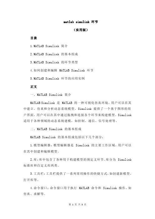
matlab simulink 环节(实用版)目录1.MATLAB Simulink 简介2.MATLAB Simulink 的基本组成3.MATLAB Simulink 的环节类型4.如何创建和编辑 MATLAB Simulink 环节5.MATLAB Simulink 环节的应用实例正文一、MATLAB Simulink 简介MATLAB Simulink 是 MATLAB 的一种可视化仿真环境,用户可以在其中建立、仿真和分析动态系统模型。
Simulink 提供了一个基于图形的用户界面,用户可以在其中通过拖拽和连接各个环节来构建模型。
Simulink 适用于各种领域的动态系统建模,如控制、通信、信号处理等。
二、MATLAB Simulink 的基本组成MATLAB Simulink 的基本组成包括以下几个部分:1.模型编辑器:模型编辑器是 Simulink 的主要工作区域,用户可以在其中创建和编辑模型。
2.库:库中包含了各种用于构建模型的预定义环节。
库分为 Simulink 标准库和自定义库两类。
3.工具栏:工具栏提供了一系列常用操作的快捷方式,如创建新模型、打开库等。
4.命令窗口:命令窗口用于执行 MATLAB 命令和 Simulink 操作,如仿真、求解等。
三、MATLAB Simulink 的环节类型MATLAB Simulink 中的环节分为以下几类:1.连续环节:表示连续时间系统,如积分器、微分器等。
2.离散环节:表示离散时间系统,如采样器、保持器等。
3.函数环节:表示各种数学函数,如线性函数、非线性函数等。
4.逻辑环节:表示逻辑运算,如与门、或门、非门等。
5.信号发生器:表示信号生成器,如正弦波发生器、脉冲发生器等。
6.接收器:表示信号接收器,如显示、记录等。
四、如何创建和编辑 MATLAB Simulink 环节在 MATLAB Simulink 中创建和编辑环节的方法如下:1.从库中选择环节:打开库,找到所需环节,单击并拖拽到模型编辑器中。

matlab与simulink设计与建模Matlab与Simulink:设计与建模Matlab是一种高级技术计算语言,广泛用于科学与工程领域。
而Simulink 是Matlab的一个应用程序,主要用于动态系统建模和仿真。
在本文中,我们将一步一步解答有关Matlab与Simulink的设计与建模的问题。
第一步:了解Matlab和Simulink的基本概念Matlab是一种用于处理矩阵和向量运算的数学软件,它具有强大的计算和数据分析能力。
Simulink是在Matlab平台上构建的一个图形化仿真环境,它通过模块和线连接来描述系统的行为。
第二步:准备工作在开始设计和建模之前,您需要安装Matlab和Simulink。
您可以从MathWorks官方网站获取免费试用版本或购买完整版本。
第三步:了解Simulink库Simulink库是Simulink软件中可用的预定义函数和模块的集合。
这些函数和模块可以用来构建系统模型。
通过浏览库,您可以找到所需的函数和模块,然后将其拖放到模型中进行使用。
第四步:创建新模型在Simulink中,您需要创建一个新模型来开始您的设计和建模工作。
在Simulink工具栏上,选择“新建模型”,然后给模型命名。
现在您可以开始在模型中添加各种组件来构建系统。
第五步:添加组件模型中的组件可以是各种类型的模块,包括数学运算器、信号生成器、传感器、控制器等。
您可以从Simulink库中选择相应的模块,并将其拖放到模型中。
第六步:连接组件在Simulink中,您可以使用线来连接模型中的各个组件。
线可以传递信号和数据,以模拟系统中不同组件之间的交互和通信。
第七步:设置模型参数每个组件都有一些参数需要设置,以便它能够正确地运行。
您可以通过右键单击组件并选择“属性”来访问组件的参数设置。
第八步:模型仿真在完成组件和参数设置后,您可以进行模型的仿真。
Simulink提供了多种仿真选项,您可以选择所需的仿真方法和参数,并开始运行仿真。
使用篇1.以管理员身份运行matlab2.登录后把当前文件夹改成C盘,找到TwinCAT→Functions→TE1400→SetupTwinCATTarget.p3.找到这个文件后右键选择Run,注意:这一步是为了选择matlabsimulink编译的module所需要的编译器种类,是第一次运行使用matlab+TE1400的时候必须执行的,以后就不必每次都操作这一步。
运行后在matlab主窗口提示让你选择是否用本地的编译器因为本地有VS2010的编译器,所以选择y后敲回车随后matlab找到本地有两种编译器,一个是matlab本体的lcc-win32 C2.4.1,另一个是VS2010,选择VS2010所代表的数字,输入2敲回车最后让matlab让你确认编译器的选择,输入y敲回车提示以下信息说明编译器选择完成4.点击工具栏中simulink图标5.弹出simulink编辑界面后,点击工具栏中的打开模型6.找到案例模型TempContrTest.mdl,点击打开7.本次案例模型是一个简单的温度控制External Setpoint是设定温度Feedback Temp是当前温度CoolerON是开关量输出8.打开simulation菜单栏,选择configuration parameters进行参数设定(1)进入参数设定后,选择右边的树形栏中的Solver,把其中的Type改成Fixed-step(2)之后选择树形栏中的Code Generation,把其中的System target file改成TwinCAT.tlc 点击Browse可以进行选择(3)继续选择树形栏中的Tc Module,在Publish module和Publish binaries for platform “TwinCAT RealTime(x86)”前打勾(4)最后选择树形栏中的Tc Advanced,把Task assignment改成Default在Add to cyclic caller,Variable cycle time,Export block digram以及Export block diagram debug information前打勾(5)以上操作完成后点击左下角的Apply(6)选择树形栏中的Code Generation,把Generate code only勾选后点击Generate code,随后matlab就开始把这个模型通过TE1400生成TC3所识别的Module了(7)回到matlab主窗口,等看到以下提示说明Module生成完成(8)我们来看下生成的Module会在什么位置可以发现在TwinCAT/3.1/CustomConfig/Modules路径下会生成名字和案例模型名字一样的文件夹TempContrTest打开可以发现里面其实主要是.tmc文件是TC3所需要的,其他都是一些描述文件,所以可以把.tmc文件拷贝出来,给一些没有Matlab的电脑上用9.打开TC3,并新建项目10.把名称改成英文,例如matlabsimulink,点击确认11.打开SYSTEM,右键TcCOM Objects添加新项12.TC3会自动找到之前生成的.tmc文件,选中后点击OK进行添加13.添加好后我们可以发现TcCOM Objects下出现matlab生成的Module,并且3个变量出现在IO位置,方便和PLC程序或者硬件IO进行变量连接14.右键Tasks添加新项名字可以改成matlab,点击OK添加新的Task15.因为我需要实施做温度计算,所以可以这个Task的优先级提高,修改成1,周期用默认的10ms即可16.双击TcCOM Objects下面的Object1(TempContrTest)Depend On改成Manual Config,并把Task分配成之前创建的名为“matlab”的Task17.右键PLC添加新项18.把名称修改为英文,例如test19.编辑一段模拟程序,模拟温度的升降20.程序写好后右键test Project,选择生成开始编译程序21.编译好后在test Instance自动生成3个变量22.接下来要做的就是把PLC中3个变量和matlab中三个变量链接起来Switch→CoolerONSP→External SetpointPV Feedback Temp23.变量链接完成后开始下传配置和程序,选择菜单栏TwinCAT,点击Activate Configuration弹出窗口点击确定提示切换到运行模式点击确定观察右下角图标是否编程绿色运行状态弹出窗口点击确定提示切换到运行模式点击确定观察右下角图标是否编程绿色运行状态24.打开PLC菜单,选择“登录到”把程序在线25.打开PLC菜单,选择“启动”把程序运行26.观察程序,看到成功利用matlab温度算法运行程序27.打开Object1(TempContrTest),选择Block Diagram也可以同时观察Matlab温度算法实时状态注:上图中可以看到由一个红色字提示说是非商业的,虽然TE1400插件装上了,但用的还是7天试用版,所以对于试用版有一些限制,查询information system可以看到如下:TC3中Scope View简单使用在之前的基础上来看下TC3下Scope View如何使用,装好TC3后Scope View会自动集成在TC3中1.首先右键“解决方案”选择添加,点击新建项目2.选择TwinCAT Measurement中的Measurement Scope Project,名称改成英文,例如tempcontrol,点击确定3.右键Axis,选择Target Browser4.打开小电脑图标下的Port_851(851),点击MAIN5.把MAIN程序中PV和SP分别添加到同一个坐标上6.保证程序在运行后,点击工具栏中的Record开始记录两个变量7.随后就可以观察到当前PV和SP的示波图下图中绿色是PV,蓝色是SP。
matlab的simulink仿真建模举例Matlab的Simulink仿真建模举例Simulink是Matlab的一个工具包,用于建模、仿真和分析动态系统。
它提供了一个可视化的环境,允许用户通过拖放模块来构建系统模型,并通过连接和配置这些模块来定义模型的行为。
Simulink是一种功能强大的仿真平台,可以用于解决各种不同类型的问题,从控制系统设计到数字信号处理,甚至是嵌入式系统开发。
在本文中,我们将通过一个简单的例子来介绍Simulink的基本概念和工作流程。
我们将使用Simulink来建立一个简单的电机速度控制系统,并进行仿真和分析。
第一步:打开Simulink首先,我们需要打开Matlab并进入Simulink工作环境。
在Matlab命令窗口中输入"simulink",将会打开Simulink的拓扑编辑器界面。
第二步:创建模型在拓扑编辑器界面的左侧,你可以看到各种不同类型的模块。
我们将使用这些模块来构建我们的电机速度控制系统。
首先,我们添加一个连续模块,代表电机本身。
在模块库中选择Continuous中的Transfer Fcn,拖动到编辑器界面中。
接下来,我们添加一个用于控制电机速度的控制器模块。
在模块库中选择Discrete中的Transfer Fcn,拖动到编辑器界面中。
然后,我们需要添加一个用于输入参考速度的信号源模块。
在模块库中选择Sources中的Step,拖动到编辑器界面中。
最后,我们添加一个用于显示模拟结果的作用模块。
在模块库中选择Sinks 中的To Workspace,拖动到编辑器界面中。
第三步:连接模块现在,我们需要将这些模块连接起来以定义模型的行为。
首先,将Step模块的输出端口与Transfer Fcn模块的输入端口相连。
然后,将Transfer Fcn模块的输出端口与Transfer Fcn模块的输入端口相连。
接下来,将Transfer Fcn模块的输出端口与To Workspace模块的输入端口相连。
simulink的modelsettingSimulink,作为MATLAB的一个重要组件,为工程师和研究人员提供了一个强大的图形化建模和仿真环境。
在Simulink中,Model Settings(模型设置)是一个关键的功能,它允许用户深入探索和自定义模型的各个方面,从而确保仿真的准确性和效率。
Model Settings提供了多种配置选项,涵盖了从基本的仿真设置到高级的优化参数。
以下是一些关键的设置及其重要性:Solver(求解器):这是模型设置中最核心的部分,它决定了仿真的时间步长和数值积分方法。
用户可以根据模型的特性和仿真需求选择合适的求解器,如固定步长、可变步长或自适应步长。
Data Import/Export(数据导入/导出):这些设置允许用户定义模型的输入和输出数据格式。
例如,用户可以选择从文件、工作区或其他数据源导入数据,并定义输出数据的格式和存储位置。
Diagnostics(诊断):通过启用诊断选项,用户可以收集有关模型仿真的详细信息,如警告、错误和性能数据。
这些信息对于调试和优化模型非常有价值。
Optimization(优化):Simulink提供了多种优化选项,以提高仿真的速度和效率。
例如,用户可以选择并行计算、自动内存管理等选项,以充分利用计算机资源并加速仿真过程。
Model Referencing(模型引用):这个设置允许用户将一个大模型分解为多个小模型,以便于管理和仿真。
通过模型引用,用户可以轻松地更新和替换子模型,而无需修改整个模型。
总之,Simulink的Model Settings为用户提供了一个全面的工具,用于配置和管理模型的各个方面。
通过深入探索这些设置,用户可以确保仿真的准确性、效率和灵活性,从而更好地满足他们的需求。
Train systemFree body diagram and Newton's lawModel ConstructionRunning the ModelObtaining M ATLAB ModelIn Simulink, it is very straightforward to represent a physical system or a model. In general, a dynamic system can be constructed from just basic physical laws. We will demonstrate through an example.Train systemIn this example, we will consider a toy train consisting of an engine and a car. Assuming that the train only travels in one direction, we want to apply control to the train so that it has a smooth start-up and stop, along with a constant-speed ride.The mass of the engine and the car will be represented by M1 and M2, respectively. The two are held together by a spring, which has the stiffness coefficient of k. F represents the force applied by the engine, and the Greek letter, mu (which will also be represented by the letter u),represents the coefficient of rolling friction.The system can be represented by following Free Body Diagrams.Page 1From Newton's law, you know that the sum of forces acting on a mass equals the mass times its acceleration. In this case, the forces acting on M1 are the spring, the friction and the force applied by the engine. The forces acting on M2 are the spring and the friction. In the vertical direction, the gravitational force is canceled by the normal force applied by the ground, so that there will be no acceleration in the vertical direction. We will begin to construct the model simply from the expressions:Sum(forces_on_M1)=M1*x1''Sum(forces_on_M1)=M1*x1''Constructing The ModelThis set of system equations can now be represented graphically, without further manipulation. First, we will construct two copies (one for each mass) of the expressions sum_F=Ma ora=1/M*sum_F. Open a new model window, and drag two Sum blocks (from the Linear library), one above the other. Label these Sum blocks "Sum_F1" and "Sum_F2".The outputs of each of these Sum blocks represents the sum of the forces acting on each mass. Multiplying by 1/M will give us the acceleration. Drag two Gain blocks into your model and attach each one with a line to the outputs of the Sum blocks.Page 2attach each one with a line to the outputs of the Sum blocks.These Gain blocks should contain 1/M for each of the masses. We will be taking these variab as M1 and M2 from the M ATLAB environment, so we can just enter the variab in the Gain blocks. Double-click on the upper Gain block and enter the following into the Gain field.1/M1Similarly, change the second Gain block to the following.1/M2Now, you will notice that the gains did not appear in the Gain blocks, and just "-K-" shows up. This is because the blocks are two small on the screen to show 1/M2 inside the triangle. The blocks can be resized so that the actual gain can be seen. To resize a block, select it by clicking on it once. Small squares will appear at the corners. Drag one of these squares to stretch the block.Page 3signal line output from the Sum blocks. Also, label these two Gain blocks "a1" and "a2".The outputs of these gain blocks are the accelerations of each of the masses. We are interested in both the velocities and the positions of the masses. Since velocity is the integral of acceleration, and position is the integral of velocity, we can generate these signals using integrator blocks. Drag two integrator blocks into your model for each of the two accelerations. Connect them with lines in two chains as shown below. Label these integrators "v1", "x1", "v2", and "x2" since these are the signals these integrators will generate.Page 4of these integrators. Label them "View_x1" and "View_x2".Now we are ready to add in the forces acting on each mass. First, you need to adjust the inputs on each Sum block to represent the proper number (we will worry about the sign later) of forces. There are a total of 3 forces acting on M1, so change the Sum_F1 block's dialog box entry to:+++There are only 2 forces acting on M2, so we can leave Sum_F1 alone for now.Page 5The first force acting on M1 is just the input force, F. Drag a Signal Generator block from the Sources library and connect it to the uppermost input of the Sum_F1 block. Label the SignalGenerator "F".The next force acting on M1 is the friction force. This force is equal to:F_friction_1=mu*g*M1*v1To generate this force, we can tap off the velocity signal and multiply by a gain, mu*g*M1.Drag a Gain block into your model window. Tap off the line coming from the v1 integrator and connect it to the input of the Gain block (draw this line in several steps if necessary). Connect the output of the Gain block to the second input of Sum_F1. Change the gain of thisPage 6Connect the output of the Gain block to the second input of Sum_F1. Change the gain of this gain block to the following.mu*g*M1Resize the Gain block to display the gain and label the gain block Friction_1.This force, however, acts in the negative x1-direction. Therefore, it must come into theSum_F1 block with negative sign. Change the list of signs of Sum_F1 to+-+The last force acting on M1 is the spring force between masses. This is equal to:Page 7The last force acting on M1 is the spring force between masses. This is equal to:k*(x1-x2)First, we need to generate (x1-x2) which we can then multiply by k to generate the force. Drag a Sum block below the rest of your model. Label it "(x1-x2)" and change its list of signs to-+Since this summation comes from right to left, we need to flip the block around. Select the bloc by single-clicking on it and select Flip from the Format menu (or hit Ctrl-F). You should see the following.Now, tap off the x2 signal and connect it to the negative input of the (x1-x2) Sum block. Tap off the x1 signal and connect it to the positive input. This will cause the lines to cross. Lines may cross, but they are only actually connected where a small block appears (such as at a tap point).Page 8Now, we can multiply this position difference by the spring constant to generate the spring force. Drag a Gain block into your model to the left of the Sum blocks. Change it's value to k and label it "spring". Connect the output of the (x1-x2) block to the input of the spring block, and the output of the spring block to the third input of Sum_F1. Change the third sign ofSum_F1 to negative (use +--).Now, we can apply forces to M2. For the first force, we will use the same spring force we just generated, except that it adds in with positive sign. Simply tap off the output of the spring block and connect it to the first input of Sum_F2.Page 9The last force to add in the the friction on M2. This is done in the exact same manner as the friction on M1, tapping off v2, multiplying by a gain of mu*g*M2 and adding to Sum_F2with negative sign. After constructing this, you should have the following.Now the model is complete. We simply need to supply the proper input and view the proper output. The input of the system will be the force, F, provided by the engine. We already have placed the function generator at the input. The output of the system will be the velocity of the engine. Drag a Scope block from the Sinks block library into your model. Tap a line off the output of the "v1" integrator block to view the output. Label the scope "View_v1".Page 10Now, the model is complete. Save your model in any file you like. You can download the completed model here.Running the ModelBefore running the model, we need to assign numerical values to each of the variab used in the model. For the train system, letM1 = 1 kgM2 = 0.5 kgk = 1 N/secF= 1 Nu = 0.002 sec/mg = 9.8 m/s^2Create an new m-file and enter the following commands.M1=1;M2=0.5;k=1;F=1;mu=0.002;g=9.8;Execute your m-file to define these values. Simulink will recognize M ATLAB variab for use in the model.Page 11the model.Now, we need to give an appropriate input to the engine. Double-click on the function generator (F block). Select a square wave with frequency .001Hz and amplitude -1 (positive amplitude steps negative before stepping positive).The last step before running the simulation is to select an appropriate simulation time. To view one cycle of the .001Hz square wave, we should simulate for 1000 seconds. Select Parameters from the Simulation menu and change the Stop Time field to 1000. Close the dialog box.Now, run the simulation and open the View_v1 scope to examine the velocity output (hit autoscale). The input was a square wave with two steps, one positive and one negative. Physically, this means the engine first went forward, then in reverse. The velocity output reflects this.Page 12Obtaining M ATLAB ModelWe can now extract a M ATLAB model (state-space or transfer function) from out simulink model. In order to do this, delete the View_v1 scope and put an Out Block (from the Connections library) in its place. Also, delete the F function generator block and put an In Block (from the Connections library) in its place. The in and out blocks define the input and output of the system we would like to extract. For a detailed description of this process and other ways of integrating M ATLAB with Simulink, click here.Save this model as train2.mdl or download our version here. Now, we can extract the model into M ATLAB. Enter the following command at the M ATLAB command window to extract a state-space model.[A,B,C,D]=linmod('train2')You should see the following output which shows a state-space model of your Simulink model.A =-0.0196 0 1.0000 -1.00000 -0.0196 -2.0000 2.00000 1.0000 0 01.0000 0 0 0B =1Page 13C =1 0 0 0D =To obtain a transfer function model, enter the following command at the M ATLAB command prompt.[num,den]=ss2tf(A,B,C,D)You will see the following output representing the transfer function of the train system.num =0 1.0000 0.0196 2.0000 0.0000den =1.0000 0.0392 3.0004 0.0588 0.0000These models are equivalent (although the states are in different order) to the model obtained by hand in the M ATLAB tutorials.Simulink ExamplesCruise Control | Motor Speed | Motor Position | Bus Suspension | Inverted Pendulum | Pitch Controller | Ball and BeamTutorialsM ATLAB Basics | M ATLAB Modeling | PID | Root Locus | Frequency Response | State Space | Digital Control | Simulink Basics | Simulink Modeling | ExamplesPage 14。