Illumination invariance and object model in content-based image and video retrieval

Object Recognition from Local Scale-Invariant FeaturesDavid G.LoweComputer Science DepartmentUniversity of British ColumbiaV ancouver,B.C.,V6T1Z4,Canadalowe@cs.ubc.caAbstractAn object recognition system has been developed that uses a new class of local image features.The features are invariant to image scaling,translation,and rotation,and partially in-variant to illumination changes and affine or3D projection. These features share similar properties with neurons in in-ferior temporal cortex that are used for object recognition in primate vision.Features are efficiently detected through a stagedfiltering approach that identifies stable points in scale space.Image keys are created that allow for local ge-ometric deformations by representing blurred image gradi-ents in multiple orientation planes and at multiple scales. The keys are used as input to a nearest-neighbor indexing method that identifies candidate object matches.Final veri-fication of each match is achieved byfinding a low-residual least-squares solution for the unknown model parameters. Experimental results show that robust object recognition can be achieved in cluttered partially-occluded images witha computation time of under2seconds.1.IntroductionObject recognition in cluttered real-world scenes requires local image features that are unaffected by nearby clutter or partial occlusion.The features must be at least partially in-variant to illumination,3D projective transforms,and com-mon object variations.On the other hand,the features must also be sufficiently distinctive to identify specific objects among many alternatives.The difficulty of the object recog-nition problem is due in large part to the lack of success in finding such image features.However,recent research on the use of dense local features(e.g.,Schmid&Mohr[19]) has shown that efficient recognition can often be achieved by using local image descriptors sampled at a large number of repeatable locations.This paper presents a new method for image feature gen-eration called the Scale Invariant Feature Transform(SIFT). This approach transforms an image into a large collection of local feature vectors,each of which is invariant to image translation,scaling,and rotation,and partially invariant to illumination changes and affine or3D projection.Previous approaches to local feature generation lacked invariance to scale and were more sensitive to projective distortion and illumination change.The SIFT features share a number of properties in common with the responses of neurons in infe-rior temporal(IT)cortex in primate vision.This paper also describes improved approaches to indexing and model ver-ification.The scale-invariant features are efficiently identified by using a stagedfiltering approach.Thefirst stage identifies key locations in scale space by looking for locations that are maxima or minima of a difference-of-Gaussian function. Each point is used to generate a feature vector that describes the local image region sampled relative to its scale-space co-ordinate frame.The features achieve partial invariance to local variations,such as affine or3D projections,by blur-ring image gradient locations.This approach is based on a model of the behavior of complex cells in the cerebral cor-tex of mammalian vision.The resulting feature vectors are called SIFT keys.In the current implementation,each im-age generates on the order of1000SIFT keys,a process that requires less than1second of computation time.The SIFT keys derived from an image are used in a nearest-neighbour approach to indexing to identify candi-date object models.Collections of keys that agree on a po-tential model pose arefirst identified through a Hough trans-form hash table,and then through a least-squaresfit to afinal estimate of model parameters.When at least3keys agree on the model parameters with low residual,there is strong evidence for the presence of the object.Since there may be dozens of SIFT keys in the image of a typical object,it is possible to have substantial levels of occlusion in the image and yet retain high levels of reliability.The current object models are represented as2D loca-tions of SIFT keys that can undergo affine projection.Suf-ficient variation in feature location is allowed to recognize perspective projection of planar shapes at up to a60degree rotation away from the camera or to allow up to a20degree rotation of a3D object.2.Related researchObject recognition is widely used in the machine vision in-dustry for the purposes of inspection,registration,and ma-nipulation.However,current commercial systems for object recognition depend almost exclusively on correlation-based template matching.While very effective for certain engi-neered environments,where object pose and illumination are tightly controlled,template matching becomes computa-tionally infeasible when object rotation,scale,illumination, and3D pose are allowed to vary,and even more so when dealing with partial visibility and large model databases.An alternative to searching all image locations for matches is to extract features from the image that are at least partially invariant to the image formation process and matching only to those features.Many candidate feature types have been proposed and explored,including line seg-ments[6],groupings of edges[11,14],and regions[2], among many other proposals.While these features have worked well for certain object classes,they are often not de-tected frequently enough or with sufficient stability to form a basis for reliable recognition.There has been recent work on developing much denser collections of image features.One approach has been to use a corner detector(more accurately,a detector of peaks in local image variation)to identify repeatable image loca-tions,around which local image properties can be measured. Zhang et al.[23]used the Harris corner detector to iden-tify feature locations for epipolar alignment of images taken from differing viewpoints.Rather than attempting to cor-relate regions from one image against all possible regions in a second image,large savings in computation time were achieved by only matching regions centered at corner points in each image.For the object recognition problem,Schmid&Mohr [19]also used the Harris corner detector to identify in-terest points,and then created a local image descriptor at each interest point from an orientation-invariant vector of derivative-of-Gaussian image measurements.These image descriptors were used for robust object recognition by look-ing for multiple matching descriptors that satisfied object-based orientation and location constraints.This work was impressive both for the speed of recognition in a large database and the ability to handle cluttered images.The corner detectors used in these previous approaches have a major failing,which is that they examine an image at only a single scale.As the change in scale becomes sig-nificant,these detectors respond to different image points. Also,since the detector does not provide an indication of the object scale,it is necessary to create image descriptors and attempt matching at a large number of scales.This paper de-scribes an efficient method to identify stable key locations in scale space.This means that different scalings of an im-age will have no effect on the set of key locations selected.Furthermore,an explicit scale is determined for each point, which allows the image description vector for that point to be sampled at an equivalent scale in each image.A canoni-cal orientation is determined at each location,so that match-ing can be performed relative to a consistent local2D co-ordinate frame.This allows for the use of more distinctive image descriptors than the rotation-invariant ones used by Schmid and Mohr,and the descriptor is further modified to improve its stability to changes in affine projection and illu-mination.Other approaches to appearance-based recognition in-clude eigenspace matching[13],color histograms[20],and receptivefield histograms[18].These approaches have all been demonstrated successfully on isolated objects or pre-segmented images,but due to their more global features it has been difficult to extend them to cluttered and partially occluded images.Ohba&Ikeuchi[15]successfully apply the eigenspace approach to cluttered images by using many small local eigen-windows,but this then requires expensive search for each window in a new image,as with template matching.3.Key localizationWe wish to identify locations in image scale space that are invariant with respect to image translation,scaling,and ro-tation,and are minimally affected by noise and small dis-tortions.Lindeberg[8]has shown that under some rather general assumptions on scale invariance,the Gaussian ker-nel and its derivatives are the only possible smoothing ker-nels for scale space analysis.To achieve rotation invariance and a high level of effi-ciency,we have chosen to select key locations at maxima and minima of a difference of Gaussian function applied in scale space.This can be computed very efficiently by build-ing an image pyramid with resampling between each level. Furthermore,it locates key points at regions and scales of high variation,making these locations particularly stable for characterizing the image.Crowley&Parker[4]and Linde-berg[9]have previously used the difference-of-Gaussian in scale space for other purposes.In the following,we describe a particularly efficient and stable method to detect and char-acterize the maxima and minima of this function.As the2D Gaussian function is separable,its convolution with the input image can be efficiently computed by apply-ing two passes of the1D Gaussian function in the horizontal and vertical directions:For key localization,all smoothing operations are done us-ingThe input image isfirst convolved with the Gaussian function usingto give a new image,B,which now has an effective smoothing of.The difference of Gaussian function is obtained by subtracting image B from A,result-ing in a ratio of between the two Gaussians.To generate the next pyramid level,we resample the al-ready smoothed image B using bilinear interpolation with a pixel spacing of1.5in each direction.While it may seem more natural to resample with a relative scale ofThe pixel differences are efficient to compute and provide sufficient accuracy due to the substantial level of previous smoothing.The effective half-pixel shift in position is com-pensated for when determining key location.Robustness to illuminationchange is enhanced by thresh-olding the gradient magnitudes at a value of0.1timesthe Figure1:The second image was generated from thefirst by rotation,scaling,stretching,change of brightness and con-trast,and addition of pixel noise.In spite of these changes, 78%of the keys from thefirst image have a closely match-ing key in the second image.These examples show only a subset of the keys to reduce clutter.maximum possible gradient value.This reduces the effect of a change in illumination direction for a surface with3D relief,as an illumination change may result in large changes to gradient magnitude but is likely to have less influence on gradient orientation.Each key location is assigned a canonical orientation so that the image descriptors are invariant to rotation.In or-der to make this as stable as possible against lighting or con-trast changes,the orientation is determined by the peak in a histogram of local image gradient orientations.The orien-tation histogram is created using a Gaussian-weighted win-dow with of3times that of the current smoothing scale. These weights are multiplied by the thresholded gradient values and accumulated in the histogram at locations corre-sponding to the orientation,.The histogram has36bins covering the360degree range of rotations,and is smoothed prior to peak selection.The stability of the resulting keys can be tested by sub-jecting natural images to affine projection,contrast and brightness changes,and addition of noise.The location of each key detected in thefirst image can be predicted in the transformed image from knowledge of the transform param-eters.This framework was used to select the various sam-pling and smoothing parameters given above,so that max-Image transformation Ori%89.0B.Decrease intensity by0.285.985.4D.Scale by0.780.383.5F.Stretch by1.565.090.3H.All of A,B,C,D,E,G.71.8 Figure2:For various image transformations applied to a sample of20images,this table gives the percent of keys that are found at matching locations and scales(Match%)and that also match in orientation(Ori%).imum efficiency could be obtained while retaining stability to changes.Figure1shows a relatively small number of keys de-tected over a2octave range of only the larger scales(to avoid excessive clutter).Each key is shown as a square,with a line from the center to one side of the square indicating ori-entation.In the second half of thisfigure,the image is ro-tated by15degrees,scaled by a factor of0.9,and stretched by a factor of1.1in the horizontal direction.The pixel inten-sities,in the range of0to1,have0.1subtracted from their brightness values and the contrast reduced by multiplication by0.9.Random pixel noise is then added to give less than 5bits/pixel of signal.In spite of these transformations,78% of the keys in thefirst image had closely matching keys in the second image at the predicted locations,scales,and ori-entationsThe overall stability of the keys to image transformations can be judged from Table2.Each entry in this table is gen-erated from combining the results of20diverse test images and summarizes the matching of about15,000keys.Each line of the table shows a particular image transformation. Thefirstfigure gives the percent of keys that have a match-ing key in the transformed image within in location(rel-ative to scale for that key)and a factor of1.5in scale.The second column gives the percent that match these criteria as well as having an orientation within20degrees of the pre-diction.4.Local image descriptionGiven a stable location,scale,and orientation for each key,it is now possible to describe the local image region in a man-ner invariant to these transformations.In addition,it is desir-able to make this representation robust against small shifts in local geometry,such as arise from affine or3D projection.One approach to this is suggested by the response properties of complex neurons in the visual cortex,in which a feature position is allowed to vary over a small region while orienta-tion and spatial frequency specificity are maintained.Edel-man,Intrator&Poggio[5]have performed experiments that simulated the responses of complex neurons to different3D views of computer graphic models,and found that the com-plex cell outputs provided much better discrimination than simple correlation-based matching.This can be seen,for ex-ample,if an affine projection stretches an image in one di-rection relative to another,which changes the relative loca-tions of gradient features while having a smaller effect on their orientations and spatial frequencies.This robustness to local geometric distortion can be ob-tained by representing the local image region with multiple images representing each of a number of orientations(re-ferred to as orientation planes).Each orientation plane con-tains only the gradients corresponding to that orientation, with linear interpolation used for intermediate orientations. Each orientation plane is blurred and resampled to allow for larger shifts in positions of the gradients.This approach can be efficiently implemented by using the same precomputed gradients and orientations for each level of the pyramid that were used for orientation selection. For each keypoint,we use the pixel sampling from the pyra-mid level at which the key was detected.The pixels that fall in a circle of radius8pixels around the key location are in-serted into the orientation planes.The orientation is mea-sured relative to that of the key by subtracting the key’s ori-entation.For our experiments we used8orientation planes, each sampled over a grid of locations,with a sample spacing4times that of the pixel spacing used for gradient detection.The blurring is achieved by allocating the gradi-ent of each pixel among its8closest neighbors in the sam-ple grid,using linear interpolation in orientation and the two spatial dimensions.This implementation is much more effi-cient than performing explicit blurring and resampling,yet gives almost equivalent results.In order to sample the image at a larger scale,the same process is repeated for a second level of the pyramid one oc-tave higher.However,this time a rather than a sample region is used.This means that approximately the same image region will be examined at both scales,so that any nearby occlusions will not affect one scale more than the other.Therefore,the total number of samples in the SIFT key vector,from both scales,is or160 elements,giving enough measurements for high specificity.5.Indexing and matchingFor indexing,we need to store the SIFT keys for sample im-ages and then identify matching keys from new images.The problem of identifyingthe most similar keys for high dimen-sional vectors is known to have high complexity if an ex-act solution is required.However,a modification of the k-d tree algorithm called the best-bin-first search method(Beis &Lowe[3])can identify the nearest neighbors with high probability using only a limited amount of computation.To further improve the efficiency of the best-bin-first algorithm, the SIFT key samples generated at the larger scale are given twice the weight of those at the smaller scale.This means that the larger scale is in effect able tofilter the most likely neighbours for checking at the smaller scale.This also im-proves recognition performance by giving more weight to the least-noisy scale.In our experiments,it is possible to have a cut-off for examining at most200neighbors in a probabilisticbest-bin-first search of30,000key vectors with almost no loss of performance compared tofinding an exact solution.An efficient way to cluster reliable model hypotheses is to use the Hough transform[1]to search for keys that agree upon a particular model pose.Each model key in the database contains a record of the key’s parameters relative to the model coordinate system.Therefore,we can create an entry in a hash table predicting the model location,ori-entation,and scale from the match hypothesis.We use a bin size of30degrees for orientation,a factor of2for scale, and0.25times the maximum model dimension for location. These rather broad bin sizes allow for clustering even in the presence of substantial geometric distortion,such as due to a change in3D viewpoint.To avoid the problem of boundary effects in hashing,each hypothesis is hashed into the2clos-est bins in each dimension,giving a total of16hash table entries for each hypothesis.6.Solution for affine parametersThe hash table is searched to identify all clusters of at least 3entries in a bin,and the bins are sorted into decreasing or-der of size.Each such cluster is then subject to a verification procedure in which a least-squares solution is performed for the affine projection parameters relating the model to the im-age.The affine transformation of a model point to an image point can be written aswhere the model translation is and the affine rota-tion,scale,and stretch are represented by the parameters.We wish to solve for the transformation parameters,so Figure3:Model images of planar objects are shown in the top row.Recognition results below show model outlinesand image keys used for matching.the equation above can be rewritten as...This equation shows a single match,but any number of fur-ther matches can be added,with each match contributing two more rows to thefirst and last matrix.At least3matches are needed to provide a solution.We can write this linear system asThe least-squares solution for the parameters x can be deter-Figure4:Top row shows model images for3D objects with outlines found by background segmentation.Bottom image shows recognition results for3D objects with model outlines and image keys used for matching.mined by solving the corresponding normal equations, which minimizes the sum of the squares of the distances from the projected model locations to the corresponding im-age locations.This least-squares approach could readily be extended to solving for3D pose and internal parameters of articulated andflexible objects[12].Outliers can now be removed by checking for agreement between each image feature and the model,given the param-eter solution.Each match must agree within15degrees ori-entation,Figure6:Stability of image keys is tested under differingillumination.Thefirst image is illuminated from upper leftand the second from center right.Keys shown in the bottomimage were those used to match second image tofirst.the top row of Figure4.The models were photographed on ablack background,and object outlinesextracted by segment-ing out the background region.An example of recognition isshown in the samefigure,again showing the SIFT keys usedfor recognition.The object outlines are projected using theaffine parameter solution,but this time the agreement is notas close because the solution does not account for rotationin depth.Figure5shows more examples in which there issignificant partial occlusion.The images in these examples are of size pix-els.The computation times for recognition of all objects ineach image are about1.5seconds on a Sun Sparc10pro-cessor,with about0.9seconds required to build the scale-space pyramid and identify the SIFT keys,and about0.6seconds to perform indexing and least-squares verification.This does not include time to pre-process each model image,which would be about1second per image,but would onlyneed to be done once for initial entry into a model database.The illumination invariance of the SIFT keys is demon-strated in Figure6.The two images are of the same scenefrom the same viewpoint,except that thefirst image is il-luminated from the upper left and the second from the cen-ter right.The full recognition system is run to identify thesecond image using thefirst image as the model,and thesecond image is correctly recognized as matching thefirst.Only SIFT keys that were part of the recognition are shown.There were273keys that were verified as part of thefinalmatch,which means that in each case not only was the samekey detected at the same location,but it also was the clos-est match to the correct corresponding key in the second im-age.Any3of these keys would be sufficient for recognition.While matching keys are not found in some regions wherehighlights or shadows change(for example on the shiny topof the camera)in general the keys show good invariance toillumination change.8.Connections to biological visionThe performance of human vision is obviously far superiorto that of current computer vision systems,so there is poten-tially much to be gained by emulating biological processes.Fortunately,there have been dramatic improvements withinthe past few years in understanding how object recognitionis accomplished in animals and humans.Recent research in neuroscience has shown that objectrecognition in primates makes use of features of intermedi-ate complexity that are largely invariant to changes in scale,location,and illumination(Tanaka[21],Perrett&Oram[16]).Some examples of such intermediate features foundin inferior temporal cortex(IT)are neurons that respond toa darkfive-sided star shape,a circle with a thin protrudingelement,or a horizontal textured region within a triangularboundary.These neurons maintain highly specific responsesto shape features that appear anywhere within a large por-tion of the visualfield and over a several octave range ofscales(Ito et.al[7]).The complexity of many of these fea-tures appears to be roughly the same as for the current SIFTfeatures,although there are also some neurons that respondto more complex shapes,such as faces.Many of the neu-rons respond to color and texture properties in addition toshape.The feature responses have been shown to dependon previous visual learning from exposure to specific objectscontaining the features(Logothetis,Pauls&Poggio[10]).These features appear to be derived in the brain by a highlycomputation-intensive parallel process,which is quite dif-ferent from the stagedfiltering approach given in this paper.However,the results are much the same:an image is trans-formed into a large set of local features that each match asmall fraction of potential objects yet are largely invariantto common viewing transformations.It is also known that object recognition in the brain de-pends on a serial process of attention to bind features to ob-ject interpretations,determine pose,and segment an objectfrom a cluttered background[22].This process is presum-ably playing the same role in verification as the parametersolving and outlier detection used in this paper,since theaccuracy of interpretations can often depend on enforcing asingle viewpoint constraint[11].9.Conclusions and commentsThe SIFT features improve on previous approaches by beinglargely invariant to changes in scale,illumination,and localaffine distortions.The large number of features in a typical image allow for robust recognition under partial occlusion in cluttered images.Afinal stage that solves for affine model parameters allows for more accurate verification and pose determination than in approaches that rely only on indexing.An important area for further research is to build models from multiple views that represent the3D structure of ob-jects.This would have the further advantage that keys from multiple viewing conditions could be combined into a single model,thereby increasing the probability offinding matches in new views.The models could be true3D representations based on structure-from-motion solutions,or could repre-sent the space of appearance in terms of automated cluster-ing and interpolation(Pope&Lowe[17]).An advantage of the latter approach is that it could also model non-rigid de-formations.The recognition performance could be further improved by adding new SIFT feature types to incorporate color,tex-ture,and edge groupings,as well as varying feature sizes and offsets.Scale-invariant edge groupings that make local figure-ground discriminations would be particularly useful at object boundaries where background clutter can interfere with other features.The indexing and verification frame-work allows for all types of scale and rotation invariant fea-tures to be incorporated into a single model representation. Maximum robustness would be achieved by detecting many different feature types and relying on the indexing and clus-tering to select those that are most useful in a particular im-age.References[1]Ballard,D.H.,“Generalizing the Hough transform to detectarbitrary patterns,”Pattern Recognition,13,2(1981),pp.111-122.[2]Basri,Ronen,and David.W.Jacobs,“Recognition using re-gion correspondences,”International Journal of Computer Vision,25,2(1996),pp.141–162.[3]Beis,Jeff,and David G.Lowe,“Shape indexing usingapproximate nearest-neighbour search in high-dimensional spaces,”Conference on Computer Vision and Pattern Recog-nition,Puerto Rico(1997),pp.1000–1006.[4]Crowley,James L.,and Alice C.Parker,“A representationfor shape based on peaks and ridges in the difference of low-pass transform,”IEEE Trans.on Pattern Analysis and Ma-chine Intelligence,6,2(1984),pp.156–170.[5]Edelman,Shimon,Nathan Intrator,and Tomaso Poggio,“Complex cells and object recognition,”Unpublished Manuscript,preprint at /edelman/mirror/nips97.ps.Z[6]Grimson,Eric,and Thom´a s Lozano-P´e rez,“Localizingoverlapping parts by searching the interpretation tree,”IEEE Trans.on Pattern Analysis and Machine Intelligence,9 (1987),pp.469–482.[7]Ito,Minami,Hiroshi Tamura,Ichiro Fujita,and KeijiTanaka,“Size and position invariance of neuronal responses in monkey inferotemporal cortex,”Journal of Neurophysiol-ogy,73,1(1995),pp.218–226.[8]Lindeberg,Tony,“Scale-space theory:A basic tool foranalysing structures at different scales”,Journal of Applied Statistics,21,2(1994),pp.224–270.[9]Lindeberg,Tony,“Detecting salient blob-like image struc-tures and their scales with a scale-space primal sketch:a method for focus-of-attention,”International Journal ofComputer Vision,11,3(1993),pp.283–318.[10]Logothetis,Nikos K.,Jon Pauls,and Tomaso Poggio,“Shaperepresentation in the inferior temporal cortex of monkeys,”Current Biology,5,5(1995),pp.552–563.[11]Lowe,David G.,“Three-dimensional object recognitionfrom single two-dimensional images,”Artificial Intelli-gence,31,3(1987),pp.355–395.[12]Lowe,David G.,“Fitting parameterized three-dimensionalmodels to images,”IEEE Trans.on Pattern Analysis and Ma-chine Intelligence,13,5(1991),pp.441–450.[13]Murase,Hiroshi,and Shree K.Nayar,“Visual learning andrecognition of3-D objects from appearance,”International Journal of Computer Vision,14,1(1995),pp.5–24. [14]Nelson,Randal C.,and Andrea Selinger,“Large-scale testsof a keyed,appearance-based3-D object recognition sys-tem,”Vision Research,38,15(1998),pp.2469–88. [15]Ohba,Kohtaro,and Katsushi Ikeuchi,“Detectability,uniqueness,and reliability of eigen windows for stable verification of partially occluded objects,”IEEE Trans.on Pattern Analysis and Machine Intelligence,19,9(1997), pp.1043–48.[16]Perrett,David I.,and Mike W.Oram,“Visual recognitionbased on temporal cortex cells:viewer-centered processing of pattern configuration,”Zeitschrift f¨u r Naturforschung C, 53c(1998),pp.518–541.[17]Pope,Arthur R.and David G.Lowe,“Learning probabilis-tic appearance models for object recognition,”in Early Vi-sual Learning,eds.Shree Nayar and Tomaso Poggio(Oxford University Press,1996),pp.67–97.[18]Schiele,Bernt,and James L.Crowley,“Object recognitionusing multidimensional receptivefield histograms,”Fourth European Conference on Computer Vision,Cambridge,UK (1996),pp.610–619.[19]Schmid,C.,and R.Mohr,“Local grayvalue invariants forimage retrieval,”IEEE PAMI,19,5(1997),pp.530–534.[20]Swain,M.,and D.Ballard,“Color indexing,”InternationalJournal of Computer Vision,7,1(1991),pp.11–32. [21]Tanaka,Keiji,“Mechanisms of visual object recognition:monkey and human studies,”Current Opinion in Neurobiol-ogy,7(1997),pp.523–529.[22]Treisman,Anne M.,and Nancy G.Kanwisher,“Perceiv-ing visually presented objects:recognition,awareness,and modularity,”Current Opinion in Neurobiology,8(1998),pp.218–226.[23]Zhang,Z.,R.Deriche,O.Faugeras,Q.T.Luong,“A robusttechnique for matching two uncalibrated images through the recovery of the unknown epipolar geometry,”Artificial In-telligence,78,(1995),pp.87-119.。

机器学习专业词汇中英⽂对照activation 激活值activation function 激活函数additive noise 加性噪声autoencoder ⾃编码器Autoencoders ⾃编码算法average firing rate 平均激活率average sum-of-squares error 均⽅差backpropagation 后向传播basis 基basis feature vectors 特征基向量batch gradient ascent 批量梯度上升法Bayesian regularization method 贝叶斯规则化⽅法Bernoulli random variable 伯努利随机变量bias term 偏置项binary classfication ⼆元分类class labels 类型标记concatenation 级联conjugate gradient 共轭梯度contiguous groups 联通区域convex optimization software 凸优化软件convolution 卷积cost function 代价函数covariance matrix 协⽅差矩阵DC component 直流分量decorrelation 去相关degeneracy 退化demensionality reduction 降维derivative 导函数diagonal 对⾓线diffusion of gradients 梯度的弥散eigenvalue 特征值eigenvector 特征向量error term 残差feature matrix 特征矩阵feature standardization 特征标准化feedforward architectures 前馈结构算法feedforward neural network 前馈神经⽹络feedforward pass 前馈传导fine-tuned 微调first-order feature ⼀阶特征forward pass 前向传导forward propagation 前向传播Gaussian prior ⾼斯先验概率generative model ⽣成模型gradient descent 梯度下降Greedy layer-wise training 逐层贪婪训练⽅法grouping matrix 分组矩阵Hadamard product 阿达马乘积Hessian matrix Hessian 矩阵hidden layer 隐含层hidden units 隐藏神经元Hierarchical grouping 层次型分组higher-order features 更⾼阶特征highly non-convex optimization problem ⾼度⾮凸的优化问题histogram 直⽅图hyperbolic tangent 双曲正切函数hypothesis 估值，假设identity activation function 恒等激励函数IID 独⽴同分布illumination 照明inactive 抑制independent component analysis 独⽴成份分析input domains 输⼊域input layer 输⼊层intensity 亮度/灰度intercept term 截距KL divergence 相对熵KL divergence KL分散度k-Means K-均值learning rate 学习速率least squares 最⼩⼆乘法linear correspondence 线性响应linear superposition 线性叠加line-search algorithm 线搜索算法local mean subtraction 局部均值消减local optima 局部最优解logistic regression 逻辑回归loss function 损失函数low-pass filtering 低通滤波magnitude 幅值MAP 极⼤后验估计maximum likelihood estimation 极⼤似然估计mean 平均值MFCC Mel 倒频系数multi-class classification 多元分类neural networks 神经⽹络neuron 神经元Newton’s method ⽜顿法non-convex function ⾮凸函数non-linear feature ⾮线性特征norm 范式norm bounded 有界范数norm constrained 范数约束normalization 归⼀化numerical roundoff errors 数值舍⼊误差numerically checking 数值检验numerically reliable 数值计算上稳定object detection 物体检测objective function ⽬标函数off-by-one error 缺位错误orthogonalization 正交化output layer 输出层overall cost function 总体代价函数over-complete basis 超完备基over-fitting 过拟合parts of objects ⽬标的部件part-whole decompostion 部分-整体分解PCA 主元分析penalty term 惩罚因⼦per-example mean subtraction 逐样本均值消减pooling 池化pretrain 预训练principal components analysis 主成份分析quadratic constraints ⼆次约束RBMs 受限Boltzman机reconstruction based models 基于重构的模型reconstruction cost 重建代价reconstruction term 重构项redundant 冗余reflection matrix 反射矩阵regularization 正则化regularization term 正则化项rescaling 缩放robust 鲁棒性run ⾏程second-order feature ⼆阶特征sigmoid activation function S型激励函数significant digits 有效数字singular value 奇异值singular vector 奇异向量smoothed L1 penalty 平滑的L1范数惩罚Smoothed topographic L1 sparsity penalty 平滑地形L1稀疏惩罚函数smoothing 平滑Softmax Regresson Softmax回归sorted in decreasing order 降序排列source features 源特征sparse autoencoder 消减归⼀化Sparsity 稀疏性sparsity parameter 稀疏性参数sparsity penalty 稀疏惩罚square function 平⽅函数squared-error ⽅差stationary 平稳性（不变性）stationary stochastic process 平稳随机过程step-size 步长值supervised learning 监督学习symmetric positive semi-definite matrix 对称半正定矩阵symmetry breaking 对称失效tanh function 双曲正切函数the average activation 平均活跃度the derivative checking method 梯度验证⽅法the empirical distribution 经验分布函数the energy function 能量函数the Lagrange dual 拉格朗⽇对偶函数the log likelihood 对数似然函数the pixel intensity value 像素灰度值the rate of convergence 收敛速度topographic cost term 拓扑代价项topographic ordered 拓扑秩序transformation 变换translation invariant 平移不变性trivial answer 平凡解under-complete basis 不完备基unrolling 组合扩展unsupervised learning ⽆监督学习variance ⽅差vecotrized implementation 向量化实现vectorization ⽮量化visual cortex 视觉⽪层weight decay 权重衰减weighted average 加权平均值whitening ⽩化zero-mean 均值为零Letter AAccumulated error backpropagation 累积误差逆传播Activation Function 激活函数Adaptive Resonance Theory/ART ⾃适应谐振理论Addictive model 加性学习Adversarial Networks 对抗⽹络Affine Layer 仿射层Affinity matrix 亲和矩阵Agent 代理 / 智能体Algorithm 算法Alpha-beta pruning α-β剪枝Anomaly detection 异常检测Approximation 近似Area Under ROC Curve／AUC Roc 曲线下⾯积Artificial General Intelligence/AGI 通⽤⼈⼯智能Artificial Intelligence/AI ⼈⼯智能Association analysis 关联分析Attention mechanism 注意⼒机制Attribute conditional independence assumption 属性条件独⽴性假设Attribute space 属性空间Attribute value 属性值Autoencoder ⾃编码器Automatic speech recognition ⾃动语⾳识别Automatic summarization ⾃动摘要Average gradient 平均梯度Average-Pooling 平均池化Letter BBackpropagation Through Time 通过时间的反向传播Backpropagation/BP 反向传播Base learner 基学习器Base learning algorithm 基学习算法Batch Normalization/BN 批量归⼀化Bayes decision rule 贝叶斯判定准则Bayes Model Averaging／BMA 贝叶斯模型平均Bayes optimal classifier 贝叶斯最优分类器Bayesian decision theory 贝叶斯决策论Bayesian network 贝叶斯⽹络Between-class scatter matrix 类间散度矩阵Bias 偏置 / 偏差Bias-variance decomposition 偏差-⽅差分解Bias-Variance Dilemma 偏差 – ⽅差困境Bi-directional Long-Short Term Memory/Bi-LSTM 双向长短期记忆Binary classification ⼆分类Binomial test ⼆项检验Bi-partition ⼆分法Boltzmann machine 玻尔兹曼机Bootstrap sampling ⾃助采样法／可重复采样／有放回采样Bootstrapping ⾃助法Break-Event Point／BEP 平衡点Letter CCalibration 校准Cascade-Correlation 级联相关Categorical attribute 离散属性Class-conditional probability 类条件概率Classification and regression tree/CART 分类与回归树Classifier 分类器Class-imbalance 类别不平衡Closed -form 闭式Cluster 簇/类/集群Cluster analysis 聚类分析Clustering 聚类Clustering ensemble 聚类集成Co-adapting 共适应Coding matrix 编码矩阵COLT 国际学习理论会议Committee-based learning 基于委员会的学习Competitive learning 竞争型学习Component learner 组件学习器Comprehensibility 可解释性Computation Cost 计算成本Computational Linguistics 计算语⾔学Computer vision 计算机视觉Concept drift 概念漂移Concept Learning System /CLS 概念学习系统Conditional entropy 条件熵Conditional mutual information 条件互信息Conditional Probability Table／CPT 条件概率表Conditional random field/CRF 条件随机场Conditional risk 条件风险Confidence 置信度Confusion matrix 混淆矩阵Connection weight 连接权Connectionism 连结主义Consistency ⼀致性／相合性Contingency table 列联表Continuous attribute 连续属性Convergence 收敛Conversational agent 会话智能体Convex quadratic programming 凸⼆次规划Convexity 凸性Convolutional neural network/CNN 卷积神经⽹络Co-occurrence 同现Correlation coefficient 相关系数Cosine similarity 余弦相似度Cost curve 成本曲线Cost Function 成本函数Cost matrix 成本矩阵Cost-sensitive 成本敏感Cross entropy 交叉熵Cross validation 交叉验证Crowdsourcing 众包Curse of dimensionality 维数灾难Cut point 截断点Cutting plane algorithm 割平⾯法Letter DData mining 数据挖掘Data set 数据集Decision Boundary 决策边界Decision stump 决策树桩Decision tree 决策树／判定树Deduction 演绎Deep Belief Network 深度信念⽹络Deep Convolutional Generative Adversarial Network/DCGAN 深度卷积⽣成对抗⽹络Deep learning 深度学习Deep neural network/DNN 深度神经⽹络Deep Q-Learning 深度 Q 学习Deep Q-Network 深度 Q ⽹络Density estimation 密度估计Density-based clustering 密度聚类Differentiable neural computer 可微分神经计算机Dimensionality reduction algorithm 降维算法Directed edge 有向边Disagreement measure 不合度量Discriminative model 判别模型Discriminator 判别器Distance measure 距离度量Distance metric learning 距离度量学习Distribution 分布Divergence 散度Diversity measure 多样性度量／差异性度量Domain adaption 领域⾃适应Downsampling 下采样D-separation （Directed separation）有向分离Dual problem 对偶问题Dummy node 哑结点Dynamic Fusion 动态融合Dynamic programming 动态规划Letter EEigenvalue decomposition 特征值分解Embedding 嵌⼊Emotional analysis 情绪分析Empirical conditional entropy 经验条件熵Empirical entropy 经验熵Empirical error 经验误差Empirical risk 经验风险End-to-End 端到端Energy-based model 基于能量的模型Ensemble learning 集成学习Ensemble pruning 集成修剪Error Correcting Output Codes／ECOC 纠错输出码Error rate 错误率Error-ambiguity decomposition 误差-分歧分解Euclidean distance 欧⽒距离Evolutionary computation 演化计算Expectation-Maximization 期望最⼤化Expected loss 期望损失Exploding Gradient Problem 梯度爆炸问题Exponential loss function 指数损失函数Extreme Learning Machine/ELM 超限学习机Letter FFactorization 因⼦分解False negative 假负类False positive 假正类False Positive Rate/FPR 假正例率Feature engineering 特征⼯程Feature selection 特征选择Feature vector 特征向量Featured Learning 特征学习Feedforward Neural Networks/FNN 前馈神经⽹络Fine-tuning 微调Flipping output 翻转法Fluctuation 震荡Forward stagewise algorithm 前向分步算法Frequentist 频率主义学派Full-rank matrix 满秩矩阵Functional neuron 功能神经元Letter GGain ratio 增益率Game theory 博弈论Gaussian kernel function ⾼斯核函数Gaussian Mixture Model ⾼斯混合模型General Problem Solving 通⽤问题求解Generalization 泛化Generalization error 泛化误差Generalization error bound 泛化误差上界Generalized Lagrange function ⼴义拉格朗⽇函数Generalized linear model ⼴义线性模型Generalized Rayleigh quotient ⼴义瑞利商Generative Adversarial Networks/GAN ⽣成对抗⽹络Generative Model ⽣成模型Generator ⽣成器Genetic Algorithm/GA 遗传算法Gibbs sampling 吉布斯采样Gini index 基尼指数Global minimum 全局最⼩Global Optimization 全局优化Gradient boosting 梯度提升Gradient Descent 梯度下降Graph theory 图论Ground-truth 真相／真实Letter HHard margin 硬间隔Hard voting 硬投票Harmonic mean 调和平均Hesse matrix 海塞矩阵Hidden dynamic model 隐动态模型Hidden layer 隐藏层Hidden Markov Model/HMM 隐马尔可夫模型Hierarchical clustering 层次聚类Hilbert space 希尔伯特空间Hinge loss function 合页损失函数Hold-out 留出法Homogeneous 同质Hybrid computing 混合计算Hyperparameter 超参数Hypothesis 假设Hypothesis test 假设验证Letter IICML 国际机器学习会议Improved iterative scaling/IIS 改进的迭代尺度法Incremental learning 增量学习Independent and identically distributed/i.i.d. 独⽴同分布Independent Component Analysis/ICA 独⽴成分分析Indicator function 指⽰函数Individual learner 个体学习器Induction 归纳Inductive bias 归纳偏好Inductive learning 归纳学习Inductive Logic Programming／ILP 归纳逻辑程序设计Information entropy 信息熵Information gain 信息增益Input layer 输⼊层Insensitive loss 不敏感损失Inter-cluster similarity 簇间相似度International Conference for Machine Learning/ICML 国际机器学习⼤会Intra-cluster similarity 簇内相似度Intrinsic value 固有值Isometric Mapping/Isomap 等度量映射Isotonic regression 等分回归Iterative Dichotomiser 迭代⼆分器Letter KKernel method 核⽅法Kernel trick 核技巧Kernelized Linear Discriminant Analysis／KLDA 核线性判别分析K-fold cross validation k 折交叉验证／k 倍交叉验证K-Means Clustering K – 均值聚类K-Nearest Neighbours Algorithm/KNN K近邻算法Knowledge base 知识库Knowledge Representation 知识表征Letter LLabel space 标记空间Lagrange duality 拉格朗⽇对偶性Lagrange multiplier 拉格朗⽇乘⼦Laplace smoothing 拉普拉斯平滑Laplacian correction 拉普拉斯修正Latent Dirichlet Allocation 隐狄利克雷分布Latent semantic analysis 潜在语义分析Latent variable 隐变量Lazy learning 懒惰学习Learner 学习器Learning by analogy 类⽐学习Learning rate 学习率Learning Vector Quantization/LVQ 学习向量量化Least squares regression tree 最⼩⼆乘回归树Leave-One-Out/LOO 留⼀法linear chain conditional random field 线性链条件随机场Linear Discriminant Analysis／LDA 线性判别分析Linear model 线性模型Linear Regression 线性回归Link function 联系函数Local Markov property 局部马尔可夫性Local minimum 局部最⼩Log likelihood 对数似然Log odds／logit 对数⼏率Logistic Regression Logistic 回归Log-likelihood 对数似然Log-linear regression 对数线性回归Long-Short Term Memory/LSTM 长短期记忆Loss function 损失函数Letter MMachine translation/MT 机器翻译Macron-P 宏查准率Macron-R 宏查全率Majority voting 绝对多数投票法Manifold assumption 流形假设Manifold learning 流形学习Margin theory 间隔理论Marginal distribution 边际分布Marginal independence 边际独⽴性Marginalization 边际化Markov Chain Monte Carlo/MCMC 马尔可夫链蒙特卡罗⽅法Markov Random Field 马尔可夫随机场Maximal clique 最⼤团Maximum Likelihood Estimation/MLE 极⼤似然估计／极⼤似然法Maximum margin 最⼤间隔Maximum weighted spanning tree 最⼤带权⽣成树Max-Pooling 最⼤池化Mean squared error 均⽅误差Meta-learner 元学习器Metric learning 度量学习Micro-P 微查准率Micro-R 微查全率Minimal Description Length/MDL 最⼩描述长度Minimax game 极⼩极⼤博弈Misclassification cost 误分类成本Mixture of experts 混合专家Momentum 动量Moral graph 道德图／端正图Multi-class classification 多分类Multi-document summarization 多⽂档摘要Multi-layer feedforward neural networks 多层前馈神经⽹络Multilayer Perceptron/MLP 多层感知器Multimodal learning 多模态学习Multiple Dimensional Scaling 多维缩放Multiple linear regression 多元线性回归Multi-response Linear Regression ／MLR 多响应线性回归Mutual information 互信息Letter NNaive bayes 朴素贝叶斯Naive Bayes Classifier 朴素贝叶斯分类器Named entity recognition 命名实体识别Nash equilibrium 纳什均衡Natural language generation/NLG ⾃然语⾔⽣成Natural language processing ⾃然语⾔处理Negative class 负类Negative correlation 负相关法Negative Log Likelihood 负对数似然Neighbourhood Component Analysis/NCA 近邻成分分析Neural Machine Translation 神经机器翻译Neural Turing Machine 神经图灵机Newton method ⽜顿法NIPS 国际神经信息处理系统会议No Free Lunch Theorem／NFL 没有免费的午餐定理Noise-contrastive estimation 噪⾳对⽐估计Nominal attribute 列名属性Non-convex optimization ⾮凸优化Nonlinear model ⾮线性模型Non-metric distance ⾮度量距离Non-negative matrix factorization ⾮负矩阵分解Non-ordinal attribute ⽆序属性Non-Saturating Game ⾮饱和博弈Norm 范数Normalization 归⼀化Nuclear norm 核范数Numerical attribute 数值属性Letter OObjective function ⽬标函数Oblique decision tree 斜决策树Occam’s razor 奥卡姆剃⼑Odds ⼏率Off-Policy 离策略One shot learning ⼀次性学习One-Dependent Estimator／ODE 独依赖估计On-Policy 在策略Ordinal attribute 有序属性Out-of-bag estimate 包外估计Output layer 输出层Output smearing 输出调制法Overfitting 过拟合／过配Oversampling 过采样Letter PPaired t-test 成对 t 检验Pairwise 成对型Pairwise Markov property 成对马尔可夫性Parameter 参数Parameter estimation 参数估计Parameter tuning 调参Parse tree 解析树Particle Swarm Optimization/PSO 粒⼦群优化算法Part-of-speech tagging 词性标注Perceptron 感知机Performance measure 性能度量Plug and Play Generative Network 即插即⽤⽣成⽹络Plurality voting 相对多数投票法Polarity detection 极性检测Polynomial kernel function 多项式核函数Pooling 池化Positive class 正类Positive definite matrix 正定矩阵Post-hoc test 后续检验Post-pruning 后剪枝potential function 势函数Precision 查准率／准确率Prepruning 预剪枝Principal component analysis/PCA 主成分分析Principle of multiple explanations 多释原则Prior 先验Probability Graphical Model 概率图模型Proximal Gradient Descent/PGD 近端梯度下降Pruning 剪枝Pseudo-label 伪标记Letter QQuantized Neural Network 量⼦化神经⽹络Quantum computer 量⼦计算机Quantum Computing 量⼦计算Quasi Newton method 拟⽜顿法Letter RRadial Basis Function／RBF 径向基函数Random Forest Algorithm 随机森林算法Random walk 随机漫步Recall 查全率／召回率Receiver Operating Characteristic/ROC 受试者⼯作特征Rectified Linear Unit/ReLU 线性修正单元Recurrent Neural Network 循环神经⽹络Recursive neural network 递归神经⽹络Reference model 参考模型Regression 回归Regularization 正则化Reinforcement learning/RL 强化学习Representation learning 表征学习Representer theorem 表⽰定理reproducing kernel Hilbert space/RKHS 再⽣核希尔伯特空间Re-sampling 重采样法Rescaling 再缩放Residual Mapping 残差映射Residual Network 残差⽹络Restricted Boltzmann Machine/RBM 受限玻尔兹曼机Restricted Isometry Property/RIP 限定等距性Re-weighting 重赋权法Robustness 稳健性/鲁棒性Root node 根结点Rule Engine 规则引擎Rule learning 规则学习Letter SSaddle point 鞍点Sample space 样本空间Sampling 采样Score function 评分函数Self-Driving ⾃动驾驶Self-Organizing Map／SOM ⾃组织映射Semi-naive Bayes classifiers 半朴素贝叶斯分类器Semi-Supervised Learning 半监督学习semi-Supervised Support Vector Machine 半监督⽀持向量机Sentiment analysis 情感分析Separating hyperplane 分离超平⾯Sigmoid function Sigmoid 函数Similarity measure 相似度度量Simulated annealing 模拟退⽕Simultaneous localization and mapping 同步定位与地图构建Singular Value Decomposition 奇异值分解Slack variables 松弛变量Smoothing 平滑Soft margin 软间隔Soft margin maximization 软间隔最⼤化Soft voting 软投票Sparse representation 稀疏表征Sparsity 稀疏性Specialization 特化Spectral Clustering 谱聚类Speech Recognition 语⾳识别Splitting variable 切分变量Squashing function 挤压函数Stability-plasticity dilemma 可塑性-稳定性困境Statistical learning 统计学习Status feature function 状态特征函Stochastic gradient descent 随机梯度下降Stratified sampling 分层采样Structural risk 结构风险Structural risk minimization/SRM 结构风险最⼩化Subspace ⼦空间Supervised learning 监督学习／有导师学习support vector expansion ⽀持向量展式Support Vector Machine/SVM ⽀持向量机Surrogat loss 替代损失Surrogate function 替代函数Symbolic learning 符号学习Symbolism 符号主义Synset 同义词集Letter TT-Distribution Stochastic Neighbour Embedding/t-SNE T – 分布随机近邻嵌⼊Tensor 张量Tensor Processing Units/TPU 张量处理单元The least square method 最⼩⼆乘法Threshold 阈值Threshold logic unit 阈值逻辑单元Threshold-moving 阈值移动Time Step 时间步骤Tokenization 标记化Training error 训练误差Training instance 训练⽰例／训练例Transductive learning 直推学习Transfer learning 迁移学习Treebank 树库Tria-by-error 试错法True negative 真负类True positive 真正类True Positive Rate/TPR 真正例率Turing Machine 图灵机Twice-learning ⼆次学习Letter UUnderfitting ⽋拟合／⽋配Undersampling ⽋采样Understandability 可理解性Unequal cost ⾮均等代价Unit-step function 单位阶跃函数Univariate decision tree 单变量决策树Unsupervised learning ⽆监督学习／⽆导师学习Unsupervised layer-wise training ⽆监督逐层训练Upsampling 上采样Letter VVanishing Gradient Problem 梯度消失问题Variational inference 变分推断VC Theory VC维理论Version space 版本空间Viterbi algorithm 维特⽐算法Von Neumann architecture 冯 · 诺伊曼架构Letter WWasserstein GAN/WGAN Wasserstein⽣成对抗⽹络Weak learner 弱学习器Weight 权重Weight sharing 权共享Weighted voting 加权投票法Within-class scatter matrix 类内散度矩阵Word embedding 词嵌⼊Word sense disambiguation 词义消歧Letter ZZero-data learning 零数据学习Zero-shot learning 零次学习Aapproximations近似值arbitrary随意的affine仿射的arbitrary任意的amino acid氨基酸amenable经得起检验的axiom公理，原则abstract提取architecture架构，体系结构；建造业absolute绝对的arsenal军⽕库assignment分配algebra线性代数asymptotically⽆症状的appropriate恰当的Bbias偏差brevity简短，简洁；短暂broader⼴泛briefly简短的batch批量Cconvergence 收敛，集中到⼀点convex凸的contours轮廓constraint约束constant常理commercial商务的complementarity补充coordinate ascent同等级上升clipping剪下物；剪报；修剪component分量；部件continuous连续的covariance协⽅差canonical正规的，正则的concave⾮凸的corresponds相符合；相当；通信corollary推论concrete具体的事物，实在的东西cross validation交叉验证correlation相互关系convention约定cluster⼀簇centroids 质⼼，形⼼converge收敛computationally计算(机)的calculus计算Dderive获得，取得dual⼆元的duality⼆元性；⼆象性；对偶性derivation求导；得到；起源denote预⽰，表⽰，是…的标志；意味着，[逻]指称divergence 散度；发散性dimension尺度，规格；维数dot⼩圆点distortion变形density概率密度函数discrete离散的discriminative有识别能⼒的diagonal对⾓dispersion分散，散开determinant决定因素disjoint不相交的Eencounter遇到ellipses椭圆equality等式extra额外的empirical经验；观察ennmerate例举，计数exceed超过，越出expectation期望efficient⽣效的endow赋予explicitly清楚的exponential family指数家族equivalently等价的Ffeasible可⾏的forary初次尝试finite有限的，限定的forgo摒弃，放弃fliter过滤frequentist最常发⽣的forward search前向式搜索formalize使定形Ggeneralized归纳的generalization概括，归纳；普遍化；判断（根据不⾜）guarantee保证；抵押品generate形成，产⽣geometric margins⼏何边界gap裂⼝generative⽣产的；有⽣产⼒的Hheuristic启发式的；启发法；启发程序hone怀恋；磨hyperplane超平⾯Linitial最初的implement执⾏intuitive凭直觉获知的incremental增加的intercept截距intuitious直觉instantiation例⼦indicator指⽰物，指⽰器interative重复的，迭代的integral积分identical相等的；完全相同的indicate表⽰，指出invariance不变性，恒定性impose把…强加于intermediate中间的interpretation解释，翻译Jjoint distribution联合概率Llieu替代logarithmic对数的，⽤对数表⽰的latent潜在的Leave-one-out cross validation留⼀法交叉验证Mmagnitude巨⼤mapping绘图，制图；映射matrix矩阵mutual相互的，共同的monotonically单调的minor较⼩的，次要的multinomial多项的multi-class classification⼆分类问题Nnasty讨厌的notation标志，注释naïve朴素的Oobtain得到oscillate摆动optimization problem最优化问题objective function⽬标函数optimal最理想的orthogonal(⽮量，矩阵等)正交的orientation⽅向ordinary普通的occasionally偶然的Ppartial derivative偏导数property性质proportional成⽐例的primal原始的，最初的permit允许pseudocode伪代码permissible可允许的polynomial多项式preliminary预备precision精度perturbation 不安，扰乱poist假定，设想positive semi-definite半正定的parentheses圆括号posterior probability后验概率plementarity补充pictorially图像的parameterize确定…的参数poisson distribution柏松分布pertinent相关的Qquadratic⼆次的quantity量，数量；分量query疑问的Rregularization使系统化；调整reoptimize重新优化restrict限制；限定；约束reminiscent回忆往事的；提醒的；使⼈联想…的（of）remark注意random variable随机变量respect考虑respectively各⾃的；分别的redundant过多的；冗余的Ssusceptible敏感的stochastic可能的；随机的symmetric对称的sophisticated复杂的spurious假的；伪造的subtract减去；减法器simultaneously同时发⽣地；同步地suffice满⾜scarce稀有的，难得的split分解，分离subset⼦集statistic统计量successive iteratious连续的迭代scale标度sort of有⼏分的squares平⽅Ttrajectory轨迹temporarily暂时的terminology专⽤名词tolerance容忍；公差thumb翻阅threshold阈，临界theorem定理tangent正弦Uunit-length vector单位向量Vvalid有效的，正确的variance⽅差variable变量；变元vocabulary词汇valued经估价的；宝贵的Wwrapper包装分类:。

基于肤色和特征相似度映射手势识别算法
江冬梅;吴晓娟
【期刊名称】《电子测量技术》
【年(卷),期】2004()2
【摘要】文中提出用来进行手区域定位和手势识别的新算法,该算法基于肤色特征和特征相似度映射函数,该函数是归一化为[0,1]的函数,它模拟在尺度空间中各点的图像特征的相似性。

实验结果表明运用该方法能够在复杂的背景中进行手势识别。

【总页数】2页(P27-28)
【关键词】手势识别;肤色;特征相似度映射;区域定位
【作者】江冬梅;吴晓娟
【作者单位】山东大学
【正文语种】中文
【中图分类】TP391.4
【相关文献】
1.基于肤色相似度和AdaBoost算法的人脸跟踪 [J], 曾宪贵;刘磊安;左文明
2.基于多相似度的条件密度手势识别跟踪算法 [J], 王丰年;戴国骏;周文晖
3.基于HSV颜色空间肤色检测算法的动态手势识别研究 [J], 李明东
4.基于肤色特征和卷积神经网络的手势识别方法 [J], 杨文斌;杨会成;鲁春;朱文博
5.基于类内最小相似度自组织映射算法及其在储层预测中的应用 [J], 鲍彬彬;吴清强
因版权原因，仅展示原文概要，查看原文内容请购买。

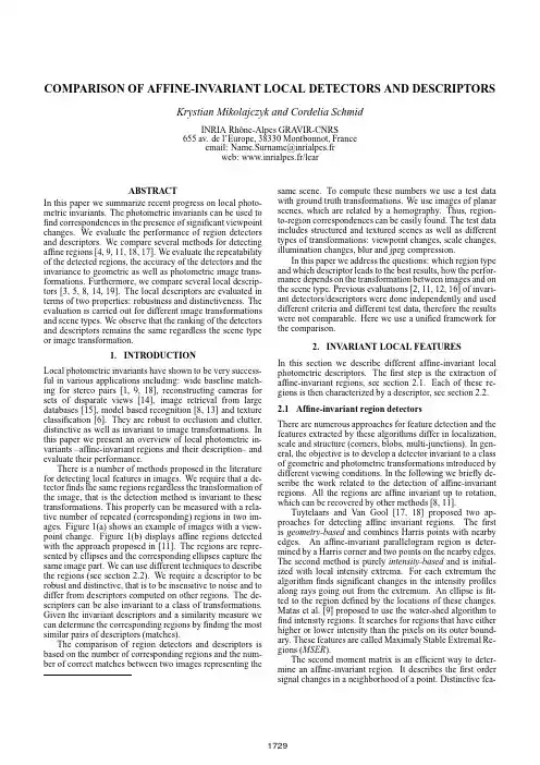
COMPARISON OF AFFINE-INV ARIANT LOCAL DETECTORS AND DESCRIPTORSKrystian Mikolajczyk and Cordelia SchmidINRIA Rhˆo ne-Alpes GRA VIR-CNRS655av.de l’Europe,38330Montbonnot,Franceemail:Name.Surname@inrialpes.frweb:www.inrialpes.fr/learABSTRACTIn this paper we summarize recent progress on local photo-metric invariants.The photometric invariants can be used tofind correspondences in the presence of significant viewpointchanges.We evaluate the performance of region detectorsand descriptors.We compare several methods for detectingaffine regions[4,9,11,18,17].We evaluate the repeatabilityof the detected regions,the accuracy of the detectors and theinvariance to geometric as well as photometric image trans-formations.Furthermore,we compare several local descrip-tors[3,5,8,14,19].The local descriptors are evaluated interms of two properties:robustness and distinctiveness.Theevaluation is carried out for different image transformationsand scene types.We observe that the ranking of the detectorsand descriptors remains the same regardless the scene typeor image transformation.1.INTRODUCTIONLocal photometric invariants have shown to be very success-ful in various applications including:wide baseline match-ing for stereo pairs[1,9,18],reconstructing cameras forsets of disparate views[14],image retrieval from largedatabases[15],model based recognition[8,13]and textureclassification[6].They are robust to occlusion and clutter,distinctive as well as invariant to image transformations.Inthis paper we present an overview of local photometric in-variants–affine-invariant regions and their description–andevaluate their performance.There is a number of methods proposed in the literaturefor detecting local features in images.We require that a de-tectorfinds the same regions regardless the transformation ofthe image,that is the detection method is invariant to thesetransformations.This property can be measured with a rela-tive number of repeated(corresponding)regions in two im-ages.Figure1(a)shows an example of images with a view-point change.Figure1(b)displays affine regions detectedwith the approach proposed in[11].The regions are repre-sented by ellipses and the corresponding ellipses capture thesame image part.We can use different techniques to describethe regions(see section2.2).We require a descriptor to berobust and distinctive,that is to be insensitive to noise and todiffer from descriptors computed on other regions.The de-scriptors can be also invariant to a class of transformations.Given the invariant descriptors and a similarity measure wecan determine the corresponding regions byfinding the mostsimilar pairs of descriptors(matches).The comparison of region detectors and descriptors isbased on the number of corresponding regions and the num-ber of correct matches between two images representing the(a)(b)Figure 1:(a)Example of test images with viewpoint change of 60.(b)Corresponding affine-invariant regions detected with Harris-Affine detector.tures are localized on strong signal changes.Lindeberg and Garding [7]developed a method for finding blob-like affine features.The authors first extract maxima of the normalized Laplacian in scale-space and then iteratively modify the scale and shape of the regions based on the second moment matrix.Affine shape estimation was used for matching and recogni-tion by Baumberg [1].He extracts Harris interest points at several scales and then adapts the shape of the point neigh-borhood to the local image structure using the iterative pro-cedure proposed by Lindeberg.The affine shape is estimated for a fixed scale and fixed location.Note that there are many points repeated at neighboring scale levels,which increases the probability of false matches as well as the complexity.Recently,Mikolajczyk and Schmid [11]proposed affine in-variant Harris-Affine and Hessian-Affine detectors.They ex-tended the scale invariant detectors [10]by the affine nor-malization.The location and scale of points are given by the scale-invariant Harris and Hessian detector.A different approach for detection of scale and affine in-variant features was proposed in [4].They search for Salient regions which locally maximize the entropy of pixel intensity distribution.2.2Region descriptorsMany different techniques for describing image regions have been recently developed.The simplest descriptor is a vector of image pixels.However,it is not invariant to different geo-metric and photometric transformations.Moreover,the high dimensionality of such a description increases the computa-tional complexity.Therefore,this technique is mainly used for finding point-to-point correspondences between two im-ages.To reduce the dimensionality the distribution of the pixel intensities can be represented by a histogram.How-ever,the spatial relations between pixels are lost and the dis-tinctiveness of such descriptor is low.Another possibility is to use a distribution of gradient orientations weighted by the gradient values within a region.Lowe [8]developed a 3D histogram,called SIFT ,where the dimensions are:gradient angle quantized to 8principal orientations and 4x4location grid on the region.Generalized moment invariants [19]have been introduced to describe the multi-spectral nature of the data.The moments characterize the shape and the intensity distribution in a region.A family of descriptors is based on Gaussian deriva-tives and can be computed to represent a point neighbor-hood [3,5].The derivatives can be computed up to a given order and normalized to be invariant to pixel intensity changes.Differential invariants and steerable filters were successfully used for image retrieval [10,15].Complex fil-ters [1,14]were designed to obtain rotation invariance andare similar to the Gaussian derivatives.In the context of tex-ture classification Gabor filters and wavelets are frequently used to describe the frequency content of an image.3.EXPERIMENTAL SETUPIn this section we describe the evaluation framework.Sec-tions 3.1and 3.2present the evaluation criteria for detectors and descriptors,respectively.In section 3.3we discuss our test data.3.1Detector evaluation criteriaThe important properties characterizing a feature detector are:the repeatability as well as the accuracy of localiza-tion and region estimation under different geometric and photometric transformations.We follow the approach pro-posed in [11]to evaluate the detectors.The repeatability score for a given pair of images is computed as the ra-tio between the number of region-to-region correspondences and the smaller number of regions detected in one of the images.We take into account only the points located in the part of the scene present in both images.Given the ground truth transformation we can find the corresponding regions.Moreover,we can project the regions from one im-age on the other and verify how closely the regions overlap.The overlap error between corresponding regions is the ratio 1of the elliptic regions and it is analytically computed using the ground truth transformation.The repeatability score depends on the arbitrary set overlap error.In this evaluation we compute the repeatability for dif-ferent overlap error.We evaluate six different detectors described in sec-tion 2.1:Harris-Affine,Hessian-Affine [11],MSER [9],In-tensity based regions [18],Geometry based regions [17]and Salient regions [4].3.2Descriptor evaluation criteriaThe regions should be repeatable,but it also very important in the matching process that the region descriptors are dis-tinctive.Distinctiveness of the descriptor is measured with the Receiver Operating Characteristics (ROC)of detection rate versus false positive rate.The detection rate is the num-ber of correct matches with respect to the number of corre-sponding regions.Two points are matched if the distance be-tween their descriptors is below an arbitrary threshold.This threshold is varied to obtain the ROC curves.We use the ground truth homography to verify if the match is correct.The false positive rate is the actual number of false matches in a database of descriptors with respect to the number of all possible false matches.The images in the database are dif-ferent from the query images,therefore all the matches in the1730database are incorrect.We compare six methods for computing region descrip-tors introduced in section2.2:SIFT descriptors[8],steerable filters[3],differential invariants[5],complexfilters[14], moment invariants[19],and cross-correlation.3.3Test dataWe evaluate the descriptors on real images1with differ-ent geometric and photometric transformations.Different changes in imaging conditions are evaluated:gradual view-point changes,scale changes,image blur,JPEG compression and illumination.We use planar scenes such that the homog-raphy can be used to determine the correctness of a match. The images contain different structured(e.g.graffiti,build-ings),or textured(e.g.trees,walls)scenes.To evaluate the false positive rate,that reflects the distinctiveness of the de-scriptors,we use a database of1000images extracted from a video.PARISON RESULTSIn the following we present the evaluation results.In sec-tion4.1we discuss the results for detectors and section4.2 for the descriptors.4.1DetectorsFigure2presents the results for the repeatability score for Graffiti images(cf.Figure1).Figure2(a)shows how the repeatability depends on the perspective transformation that the image undergoes.For a given overlap error of50%(de-tection accuracy)we increase the transformation between the reference image and the query image and measure the rela-tive number of corresponding regions.We can observe that the performance decreases for large viewpoint angles.Fig-ure2(b)displays the actual number of corresponding features with the overlap error of50%.We require a detector to have a high repeatability score and a large number of correspondences.For most trans-formations and scene types the MSER,Harris-Affine and Hessian-Affine regions obtain the best repeatability score. Harris and Hessian detector provide several times more cor-responding regions than the other detectors but this number decreases for larger transformations between images.Figure2(c)shows the repeatability score computed for a pair of images with a viewpoint change of50degrees.We compute the repeatability score while varying the overlap error.The threshold rejects the corresponding regions de-tected with larger overlap error(lower accuracy).A high score for a small overlap error indicates a high accuracy of a detector.In all test MSER and Intensity based regions ob-tain higher repeatability score than other detectors for a small overlap error.The number of corresponding regions detected with Harris-Affine and Hessian-Affine significantly increases when larger overlap error is allowed.4.2DescriptorsIn the following we discuss the results for descriptors eval-uation.Figure3(a)shows the detection rate with respect to false positive rate.Figure3(a)shows the results for a viewpoint change of the Graffiti sequence.Examples for other image transfor-mations can be found in[12].In all tests,except for light(a)(b)(c)Figure2:Evaluation of the affine detectors.(a)Repeatability score for an increasing viewpoint change.(b)Number of corresponding regions in the images.(c)Repeatability score for increasing overlaperror.(a)(b)Figure3:Descriptor evaluation.(a)ROC for different local descriptors computed on Harris-Affine regions.(b)Matching score for SIFT descriptor computed on different region types with respect to viewpoint changes.[3]W.Freeman and E.Adelson.The design and use of steerablefilters.IEEE Transactions on Pattern Analysis and MachineIntelligence,13(9):891–906,1991.[4]T.Kadir and A.Zisserman.An affine invariant detector.InProceedings of the8th European Conference on ComputerVision,Pague,Tcheque Republic,2004.[5]J.Koenderink and A.van Doorn.Representation of local ge-ometry in the visual system.Biological Cybernetics,55:367–375,1987.[6]zebnik,C.Schmid,and J.Ponce.Sparse texture rep-resentation using affine-invariant neighborhoods.In Pro-ceedings of the Conference on Computer Vision and PatternRecognition,Madison,Wisconsin,USA,2003.[7]T.Lindeberg and J.Garding.Shape-adapted smoothing inestimation of3-D shape cues from affine deformations of lo-cal2-D brightness structure.Image and Vision Computing,15(6):415–434,1997.[8]D.G.Lowe.Object recognition from local scale-invariantfeatures.In Proceedings of the7th International Conferenceon Computer Vision,Kerkyra,Greece,pages1150–1157,1999.[9]J.Matas,O.Chum,M.Urban,and T.Pajdla.Robust widebaseline stereo from maximally stable extremal regions.InProceedings of the13th British Machine Vision Conference,Cardiff,England,pages384–393,2002.[10]K.Mikolajczyk and C.Schmid.Indexing based on scale in-variant interest points.In Proceedings of the8th InternationalConference on Computer Vision,Vancouver,Canada,pages525–531,2001.[11]K.Mikolajczyk and C.Schmid.An affine invariant interestpoint detector.In Proceedings of the7th European Confer-ence on Computer Vision,Copenhagen,Denmark,volume I,pages128–142,May2002.[12]K.Mikolajczyk and C.Schmid.A performance evaluation oflocal descriptors.In Proceedings of the Conference on Com-puter Vision and Pattern Recognition,Madison,Wisconsin,USA,June2003.[13]F.Rothganger,zebnik,C.Schmid,and J.Ponce.3D ob-ject modeling and recognition using affine-invariant patchesand multi-view spatial constraints.In Proceedings of the Con-ference on Computer Vision and Pattern Recognition,Madi-son,Wisconsin,USA,2003.[14]F.Schaffalitzky and A.Zisserman.Multi-view matchingfor unordered image sets.In Proceedings of the7th Eu-ropean Conference on Computer Vision,Copenhagen,Den-mark,2002.[15]C.Schmid and R.Mohr.Local grayvalue invariants for imageretrieval.IEEE Transactions on Pattern Analysis and MachineIntelligence,19(5):530–534,May1997.[16]C.Schmid,R.Mohr,and C.Bauckhage.Evaluation of inter-est point detectors.International Journal of Computer Vision,37(2):151–172,2000.[17]T.Tuytelaars and L.V.Gool.Content-based image retrievalbased on local affinely invariant regions.In Int.Conf.on Vi-sual Information Systems,pages493–500,1999.[18]T.Tuytelaars and L.Van Gool.Wide baseline stereo matchingbased on local,affinely invariant regions.In The EleventhBritish Machine Vision Conference,University of Bristol,UK,pages412–425,2000.[19]L.Van Gool,T.Moons,and D.Ungureanu.Affine/photo-metric invariants for planar intensity patterns.In Proceedingsof the4th European Conference on Computer Vision,Cam-bridge,England,pages642–651,1996.1732。

1. 导言OpenCV（Open Source Computer Vision）是一个开源的计算机视觉库，提供了丰富的图像处理和计算机视觉算法，包括图像处理、特征检测、目标跟踪等功能。

其中，homography函数是OpenCV中的一个重要功能，用于实现图像的透视变换与投影变换。

2. 什么是homographyHomography，又称单应性矩阵，是指在单个视平线下的透视投影变换矩阵。

在计算机视觉中，homography通常用于处理多个视角下的图像对准和重叠。

通过计算homography矩阵，可以实现图像的透视变换、图像配准等功能。

3. homography函数的基本用法在OpenCV中，homography函数的基本用法需要包括以下步骤：1）利用特征匹配算法找到两幅图像中对应的特征点；2）根据这些特征点，利用findHomography函数计算出homography矩阵；3）利用warpPerspective函数将图像进行透视变换，实现图像的对齐和重叠。

4. homography函数在图像配准中的应用图像配准是计算机视觉中的重要任务之一，其目的是将多幅图像对齐到同一坐标系中，以便进行后续的特征提取、目标跟踪等操作。

homography函数在图像配准中具有重要的应用价值，可以帮助实现图像的对齐和重叠。

5. homography函数在视觉SLAM中的应用视觉SLAM（Simultaneous Localization and Mapping）是指通过相机等传感器获取环境信息，实现同时定位和地图构建的技术。

在视觉SLAM中，homography函数可以用于处理传感器获得的图像数据，实现地图的构建和定位的精准计算。

6. homography函数的高级用法除了基本的图像配准和SLAM应用外，homography函数还可以应用于其他领域，如虚拟现实、增强现实等。

通过计算homography矩阵，可以实现图像的透视变换和投影变换，为图像处理和计算机视觉领域提供了强大的功能支持。

Dense Interest PointsTinne TuytelaarsK.U.Leuven,ESAT-PSI Tinne.Tuytelaars@esat.kuleuven.beAbstractLocal features or image patches have become a stan-dard tool in computer vision,with numerous application domains.Roughly speaking,two different types of patch-based image representations can be distinguished:interest points,such as corners or blobs,whose position,scale and shape are computed by a feature detector algorithm,and dense sampling,where patches offixed size and shape are placed on a regular grid(possibly repeated over multiple scales).Interest points focus on‘interesting’locations in the image and include various degrees of viewpoint and illu-mination invariance,resulting in better repeatability scores. Dense sampling,on the other hand,gives a better coverage of the image,a constant amount of features per image area, and simple spatial relations between features.In this pa-per,we propose a hybrid scheme,which we call dense in-terest points,where we start from densely sampled patches yet optimize their position and scale parameters locally.We investigate whether doing so it is possible to get the best of both worlds.1.IntroductionRecent progress in thefield of object and scene recogni-tion has shown that good image representations are crucial when it comes to learning high level concepts from images. Even the best learning mechanisms cannot easily make up for bad features,also known as the‘garbage in,garbage out’principle.In this paper,we inspect two of the most com-monly used low-level image representations:interest points and dense sampling on a regular grid.We look at their re-spective strengths and weaknesses,and propose a hybrid scheme,dense interest points,combining the best of both worlds.When the goal is to recognize specific objects or tofind correspondences between two or more wide baseline views of the same scene,viewpoint invariant interest points,such as corners or blobs are to be preferred(see[22]for a re-cent survey of these methods).This is also the application domain for which interest point detectors were originallyter,the same interest point detectors have also been applied successfully in the context of category-level object recognition,scene classification and image un-derstanding(e.g.[7,9,19]).However,more and more re-searchers have switched to a much simpler scheme recently, which turns out to work just as well in this new context, namely dense sampling of the image with a regular grid, possibly over a range of scales(e.g.[6,20,23]).Nowak et al.[4]have shown that in the context of category-level ob-ject recognition the density of extracted features is the dom-inant factor in determining the recognition performance, while the repeatability of the individual features(in their study interest points versus random patches)plays only a secondary role.In the recent Pascal Visual Object Classes Challenges[5],it has been shown that the best performance is obtained by using a combination of both interest points and densely sampled image patches.Interest points yield a high repeatability,i.e.they can be extracted reliably and are often found again at similar lo-cations in other images of the same object or scene.Also, with interest points the user can choose the appropriate level of viewpoint and illumination invariance,depending on the application and expected variability.As the name suggests, interest point detectors focus on‘interesting’regions,which are typically regions with high information content,that can be localized precisely.These are in some sense optimal when the goal is tofind correspondences between two views of the same object or scene.However,when the goal is image interpretation,it is unclear whether the heuristics on which these feature extraction methods are based actually perform a good feature selection task or not.On the downside,the number of interest points extracted from an image varies a lot based on the image content–of-ten from a few hundred to several thousands without chang-ing the parameters.Sometimes,when the contrast in an im-age is low,not a single interest point is found,making the image representation useless.Dense sampling on a regular grid,on the other hand,re-sults in a good coverage of the entire object or scene and a constant amount of features per image area.Regions with less contrast contribute equally to the overall image rep-1original image dense sampling dense interest points interest pointsFigure1.Dense interest points,as proposed in this paper,(middle)form a hybrid scheme in between dense sampling on a regular grid (left)and interest point detection(right),combining(to some extent)the good coverage and(semi)regularity of dense sampling with the repeatability of interest points.resentation.This is based on the idea that,even if suchpatches cannot be matched accurately,they do contain valu-able information regarding the image content,that may helpto interpret the scene.Also,spatial relations between fea-tures follow a regular pattern that is easily represented ina simple model.This is important when using Markov orconditional randomfields or when modelling the spatialconfiguration of features.This does not hold for interestpoints,where spatial relations are more arbitrary and,as aconsequence,incorporating information on the spatial con-figuration is more complicated.For instance,consider thedefinition of the concept of‘neighbours’.Sivic et al.haveproposed taking the N nearest neighbours[18],but theseare in some cases quite far away.Alternatively,one can useall interest points within a certain radius around the giveninterest point,but then the number of neighbours can varygreatly.On the downside,dense sampling cannot reach the samelevel of repeatability as obtained with interest points,un-less sampling is performed extremely densely–but then thenumber of features quickly grows unacceptably large.Inpractice,researchers often use an overlap between patchesof50%or less.This is clearly not enough to guarantee simi-lar descriptors in case of structured scenes,especially whencombined with SIFT-like descriptors[12],which further di-vide the region in smaller subpatches(in spite of SIFTs ro-bustness to small misalignments).Dense Interest Points,i.e.the hybrid scheme proposedin this paper,is our attempt to combine the advantagesof both schemes.We start from densely sampled imagepatches and then apply for each feature a local optimizationof the position and scale within a bounded search area.Thisway,we get dense coverage of the entire scene and clearlydefined spatial relations,as in the case of dense sampling,yet with improved repeatability,as in the case of interestpoints(see alsofigure1).Related Work To the best of our knowledge,no hybridfeature extraction schemes combining ideas from interestpoint detection with ideas from dense sampling have beenproposed to date in the context of object recognition or im-age understanding.When searching for stereo correspon-dences,however,it is common practice to divide the imagein a small number of subareas and adapt the threshold of theinterest point detector so as to ensure that a similar numberof features is found in each subarea(e.g.[16]).This guar-antees that the features are well distributed over the entireimage,which results in a more accurate camera calibration.The dense interest points proposed here can be consideredas an extreme case of this idea,where the subareas havebeen made so small they each contain one and only one fea-ture,and with the extension that also the scale dimensionis taken into account.It is only in this extreme case thatthe benefits of preserving the(semi-)regular grid structureappear.Similarly,in their image stitching work,Brown et al.[2]introduce the concept of adaptive non-maximal suppres-sion.Instead of selecting features based on a thresholdon the corner strength,they increase the radius of the non-maximal suppression,avoiding nearby detections and henceresulting in a better distribution of the features over the im-age.Still,large portions of the image may not have a singlefeature,and again there is no(semi-)regularity in the featuredistribution.Tola et al.have proposed a scheme for efficiently com-puting dense descriptors[20].However,they do not changethe detection scheme,sticking to the traditional sampling ona regular grid.So their work can be seen as complementaryto ours.Finally,apart from regular grids,some authors have pro-posed to use random sampling(e.g.[13,4]),but this doesnot seem to have any advantage over regular grids,andequally ignores the actual image content during the featureextraction process.The rest of the paper is organized as follows.First,we describe in more detail how we extract dense interest points and discuss their main properties(section2).Next,we ex-perimentally validate the usefulness of such features,both with respect to repeatability as well as in the context of a classification and matching application(section3).Sec-tion4concludes the paper.2.Dense Interest PointsThe starting point for our dense interest points consists of a set of patches densely sampled on a regular grid over multiple scales.For larger scales,a coarser grid is used, such that the overlap ratio between neigbouring patches re-mains(approximately)fixed.This can also be thought of as applying the same grid to multiple downscaled versions of the original image in a scalespace pyramid.Next,each of the patches so obtained is further refined, both with respect to its location as with respect to its scale. To this end,any measure of‘interestingness’proposed in the context of interest point detection can be used,such as the Harris cornerness measure,the determinant of the Hes-sian,the Laplacian,or saliency based on entropy.The re-finement consists of searching for a local maximum within a bounded search area.This search area reaches up to the boundaries of the search areas of the neighbouring patches, both spatially as well as over scales.This gives us the max-imal freedom to adapt to the image content while still keep-ing the topological structure of the original regular grid in-tact.In our implementation,we have chosen the Laplacian as optimization criterion.When the goal is tofind stable fea-tures,the Laplacian is often criticized because itfinds too many features on edges,which are not well localized.How-ever,in an image understanding context,the goal is tofind representative features rather than stable ones.If within a bounded search area an edge is the most prominent feature, we want the refinement process to center the patch onto this edge,even if this results in an unstable localization.Hence the Laplacian seems to be a good choice.Of course,it cannot be guaranteed that a true local max-imum is found within such a limited search area,e.g.if the function to be maximized is monotonously increasing.In such cases,a point on the boundary of the search area is selected.One may argue that this is suboptimal,since it de-pends on the discretization imposed by the underlying reg-ular grid.However,it is not any worse than selecting the center point,as is done when sampling patches on a regular grid without refinement.If the function to be maximized is constant over the entire search area,the refinement process selects the center point(or it is determined randomly,based on the noise in the signal).2.1.Implementation detailsIn our implementation,we deviated slightly from the tra-ditional scale space pyramid.Within each octave,we keep the size of the images constant and vary the sigma of the Laplacian-of-Gaussian instead.This results in rectangular search areas and hence a slightly simpler implementation. However,note that this is just an implementation choice and not inherent to the use of dense interest points.Fig-ure2sketches the core of the algorithm and its relation to the standard Laplacian-of-Gaussians(LoG)scheme as well as to dense sampling on a regular grid.First,we build a LoG scale pyramid.Here,we typically use more pyramid levels per octave than usual(16in our experiments).The standard LoG feature extraction process then checks for each pixel whether it is a local maximum in a3×3×3neighbour-hood(spatially and over scales).Only if a true local max-imum is found,is the pixel retained as interest point(and further refined using parabolic interpolation).This process is repeated for each pixel,each time checking whether it is a local maximum in a small(3×3×3)neigbourhood. Instead,we look for maxima in larger search areas,span-ning multiple scales and extending beyond the direct neigh-bouring pixels.The size of these search areas is determined based on the underlying regular grid:each search area cor-responds to the V oronoi cell around a vertex of the regular grid.For instance,when using a grid consisting of patches at the lowest scale of size32×32with50%overlap be-tween patches and2scales per octave,the distance between two neighbouring vertices is16pixels and the search area is16pixels×16pixels×8scale levels(assuming16scale levels per octave).However,in contrast to the standard LoG scheme,the maximum found within such a search area is always retained as dense interest point,even if it is not a local maximum.This may happen for maxima found on the boundary of the search region.Similarly,even if there are multiple local maxima within the search area,only one dense interest point per search area is retained.As a re-sult,even though our search areas are much larger and non-overlapping,we typicallyfind a larger number of features. In fact,the number of features isfixed and corresponds to the number of vertices of the regular grid.With more scale levels per octave,we can determine the scale of the dense interest points accurately,without having to rely on parabolic interpolation.It is important to stress here that the proposed method is by no means limited to this framework of a Laplacian of Gaussians pyramid.As mentioned before,any interest point detection method that is based onfinding a local maximum of a measure for interestingness can be extended to dense interest point detection.ScaleScale(this paper)LoG interest points LoG dense interest points Dense samplingon a regular gridFigure2.Illustration how dense interest points can be computed using a Laplacian-of-Gaussians scale pyramid.Local maxima are searched within largerneighbourhoods than the3×3×3neighbourhoods used by standard interest point detection schemes.Moreover,we always keep exactly one feature per search neighbourhood.Instead of LoG,other interest measures can be used as well.dense sampling dense interest points interest pointsFigure3.Unlike dense sampling on a regular grid(left)dense interest points(middle),like standard interest points(right),adapt to the underlying image structure,so they can center on important features in the image,like the eyes,nose tip,nose ridge and mouth corners of the face(top)or the lights or prints of the car(bottom)(highlighted using colour coding).Likewise,this adaptation ensures that similar patches are extracted on the two halves of these symmetric objects(zoomed in and only a single scale layer for clarity).2.2.DiscussionFigure3shows some of the patches extracted both withand without this refinement step,ing the newly pro-posed dense interest points and based on dense samplingon a regular grid,as well as the result of a standard inter-est point detector(Hessian Laplace[14]).As can be seenfrom thefigure,the configuration of dense interest points isless regular than the result of dense sampling,yet they stilldensely cover the entire image in contrast to the HessianLaplace features,which for thefirst example focus more onthe background than on the foreground object.Moreover,when there is a prominent feature in the image,such as theeyes,nose tip,nose ridge,or mouth corners for the face,orthe lights or prints for the car,there is a good chance thatone of the dense interest points locks onto it.Note that thisalso holds for the nose ridge,which was not found with thestandard interest point detector,due to the lack of contrast.As a result,similar features are found for both halves ofthese symmetric objects(see alsofigure4).From these ob-Figure4.Some example patches extracted with dense interestpoints(with some of the second and fourth row patches mirrored,to highlight the similarity between patches extracted from sym-metric locations).servations,it can be expected that also for different viewsof the same object a higher repeatability is obtained.Some statistics Closer inspection of the refinement pro-cedure at work reveals that only for a very small fraction ofthe features a true local maximum over space and scale isfound(on the order of one percent,depending on the imagecontent and the density of the grid).For another two out ofevery three features,approximately,a local maximum overspace is reached,but not over scale.For the remaining30%,the refinement procedure yields a feature on the boundaryof the search area.However,this also depends on the rel-ative scale of the sigma of the LoG relative to the size ofthe search neighbourhoods.We expect that with a smallervalue for sigma,more true local maxima will be found.Spatial structure Figure5shows some examples of theoriginal regular grid(left)and the deformed version afterrefinement(middle),with vertices corresponding to the cen-ters of features.The topological structure is preserved,eventhough the grid itself is deformed,adapting to the actual im-age content.Sometimes,two vertices end up very close toeach other.This happens when a local maximum is locatedon or near a boundary between two search areas.Furthernote how the refinement procedure tries to align the gridvertices with interesting structures in the image,includingnot only blobs,but also edges,ridges,and symmetry axes.Even though we only show the grid for a single scale level,it is actually a3D grid structure in a scalespace volume,alsolinking overlapping patches at different scale levels.Since the topological structure of the original regulargrid is kept intact,spatial relations such as‘left of’,‘rightof’,‘above’,‘below’,‘4-neighbours’or‘8-neighbours’with respect to the grid are preserved and can be exploitede.g.when using a Markov or conditional randomfield.Alsowhen modelling spatial configurations in general,such gridstructure can be useful.For instance,one can define pairsof features that are separated by afixed number of edge seg-ments–e.g.infigure5,the mouth corner and eye are aboveeach other and four grid lengths apart from each other andtogether can form an interesting,more discriminative fea-ture(e.g.in a freqent itemset mining context as in[21]).So far,we looked at the grid as providing links or spatialrelations between features,but one can also consider the‘patches’formed by the quadrangles of the grid.These aresomewhat reminiscent of superpixels[17],albeit not basedon color segmentation and preserving the regular structurewe alsofind with normal pixels.When using standard interest points,one can approxi-mate these results by computing a Delaunay triangulation(seefigure5,right).However,the obtained triangles varya lot in scale and are sometimes very elongated,linking faraway points.There is also no regularity in the obtained gridstructure in this case.3.Experimental EvaluationWe validate the usefulness,strengths and weaknesses ofthe newly proposed image representation in three experi-mental setups.First,we evaluate the repeatability underscale,rotation and viewpoint variations.Next,we evalu-ate the new features in the context of a classification andmatching task.For all these experiments,we use the same set of param-eters.We start from a regular grid with50%overlap be-tween neighbouring patches and two scales per octave,withthe smallest scale corresponding to32×32patches and in-creasing scales over4octaves.For a typical Pascal VOCchallenge image,this results in around1000features perimage.The optimization criterion for the refinement step isthe Laplacian.Features are described with SIFT[12],withone tiny modification:we only normalize the features if theoriginal norm is larger than one,otherwise,we keep the fea-ture descriptor without normalization.This is necessary toavoid blowing up noise for features extracted on homoge-neous image areas.3.1.RepeatabilityFirst,we evaluate the repeatability of the newly proposedfeatures.To this end,we use some of the standard bench-marking sequences as well as the evaluation protocol pro-posed and made available by[15].We compare our denseinterest points with patches extracted by dense sampling onthe same regular grid,and with the Hessian-Laplace scale-invariant interest point detector of[14].The results areshown infigure6.Clearly,dense interest points do not reachdense sampling dense interest points interest pointsFigure5.The grid structure of the regular dense sampling that was used as initialization(left)can be transferred to the dense interest points (middle)and provides spatial structure information such as neighbours.(vertices correspond to the center of extracted patches;only a single scale layer for clarity).For standard interest points(here Hessian Laplace,right),one can compute a Delaunay triangulation,but this sometimes connects far away points and lacks regularity.the same level of repeatability as standard interest points. This comes as no surprise,since on more or less homoge-neous areas in the image,our dense interest point detector is forced to make a selection,even though there is no in-formation available to ensure a stable and repeatable selec-tion.This is especially noticeable for the Bark sequence, where contrast is often relatively low.However,they score significantly better than the features found by dense sam-pling.When repeatability is the sole criterion(e.g.when the goal is tofind correspondences between images),there is no doubt that standard interest points are to be preferred over our dense interest points.However,when representa-tive features are sought for,dense interest points may be a good choice,as they select repeatable features where pos-sible,combined with unstable,yet still informative features elsewhere.3.2.ClassificationNext,we evaluate the performance of our dense interest points in the context of a classification task.Here,we focus on a comparison with dense sampling on a regular grid,as this strategy has been shown to outperform interest points in this context(see e.g.[8]or the feature comparison per-formed in the context of the CVPR09Features workshop[1] ).As in[1],we use the Pascal VOC2007dataset[5].All features arefirst vector quantized.For this,we use k-means run on a subset of the data.Already at this point,we can ob-serve a difference between dense interest points and dense sampling on a regular grid:for the same number of features and the same number of clusters,the obtained clustersare Figure6.Repeatability of dense interest points(green diamonds), dense sampling on a regular grid(red triangles),and Hes-sian Laplace(blue squares),for the Boat(scale+rotation),Bark (scale+rotation)and Graffiti(viewpoint changes)sequences. more compact for the dense interest points,with the sum of squared error output of the clustering algorithm about5-10%smaller.We experimented with visual vocabularies of size500, 1000,2000,and4000.In most cases,the best results were obtained with the largest vocabularies.Images are repre-aeroplane bicycle bird boat bottle bus car dense sampling61.9947.4430.6246.1922.6837.9361.56 dense interest points63.7549.2431.8350.0223.2337.6463.19cat chair cow diningtable dog horse motorbike dense sampling37.0143.9023.3228.1833.3057.0047.04 dense interest points39.6844.7629.0831.3531.4859.9347.22person pottedplant sheep sofa train tvmonitor avg dense sampling74.7013.8719.9435.4752.3931.9240.32 dense interest points75.3513.7830.7435.5357.5237.1942.63 Table1.Results on the Pascal VOC2007data(measured by average precision).sented with a bag-of-features representation,ignoring any spatial information.Then,a support vector machine is trained(using[3]),with aχ2-kernel and determining the optimal parameters on the validation set.The results,mea-sured by average precision following the Pascal VOC2007 protocol,are summarized in table1.For15out of the20classes,dense interest points outper-form the dense sampling.Only for dogs does dense sam-pling perform better than dense interest points.Averaged out over all20classes,we get an increase in mean average precision of more than2%compared to dense sampling.We realize these results are inferior to the winning schemes in the Pascal VOC challenge.However,we used a very stan-dard,baseline scheme(not using any spatial information, not using multiple kernels,etc.).The purpose of this exper-iment is to compare the performance of the different image representations on a standard dataset,not to compete with these more complex systems.In fact,our results are quite competitive when compared to those reported in the study performed at the CVPR2009features workshop[1].We would probably rank among the topfive best performing methods,and are probably the only scheme scoring so high without using color information or extracting significantly larger numbers of features.3.3.MatchingFinally,we show some preliminary results on an image matching task.Recently,Liu et al.have proposed SIFTflow, a scheme to align different images of similar scenes[11]. For each pixel in the image,they compute a SIFT-descriptor. Then,an opticalflow like algorithm is used to bring the im-ages into alignment.This works amazingly well,as long as the two images are sufficiently similar(‘dense sampling in the space of world images’,as they call it).Still,their approach has some limitations.To make it work,SIFT de-scriptors need to be extracted at each and every pixel in the image.At the same time,to keep the memory requirements under control,the total number of descriptors cannot be too large.To this end,they downscale the image significantly. This results in a loss of detail(smoothing).Moreover,the extracted descriptors end up covering a relatively large part of the image,often containing parts of different scene ob-jects.Finally,descriptors are only computed at a single scale.Changes in scale can only be dealt with in as far as they can be covered by the robustness that comes with SIFT.These constraints arefine when the two images in-deed have very similar scene compositions.However,they may be broken when the difference between the images gets larger.The obtained results are good enough for comput-ing a precise scene similarity score[11]or for transferring annotations[10].However,the warped images look rather patchy,with artefacts due to discontinuities in theflowfield.Instead,we propose to extract dense interest points on the original image(not downscaled).The precise position and scale of each feature(within a certain range)are de-termined based on the image content.Descriptors can make use of all the information present in the image,as there is no need for smoothing or downscaling.Also,they can be kept relatively small(the same size as typically used in object recognition experiments),limiting the disturbing effect of occlusions or background objects.Some preliminary results are shown infigure7.These results were obtained using the code provided by Liu et al.,replacing their SIFT computa-tion by our dense interest point computation.We did not use the hierarchical extension,as in our experiments this had a negative effect on the quality of the result.Clearly,the use of dense interest points allowsfiner detail of the image to be preserved and obtain a better reconstruction.4.Conclusion and Future WorkIn this paper we have introduced dense interest points,a hybrid scheme in between dense sampling on a regular grid and interest point detection.We start from image patches sampled on a regular grid,but then refine their position and scale by optimizing an‘interestingness’measure(in our im-plementation the Laplacian).This results in a set of interest points on a semi-regular grid,densely covering the entire image as is the case with dense sampling,but with repeata-bility properties closer to those of standard interest points.Several extensions and variations on this basic scheme。

Automatic Panoramic Image Stitching using Invariant FeaturesMatthew Brown and David G. Lowe{mbrown|lowe}@cs.ubc.caDepartment of Computer Science,University of British Columbia,Vancouver, Canada.AbstractThis paper concerns the problem of fully automated panoramic image stitching. Though the 1D problem (single axis of rotation) is well studied, 2D or multi-row stitching is more difficult. Previous approaches have used human input or restrictions on the image sequence in order to establish matching images. In this work, we formulate stitching as a multi-image matching problem, and use invariant local features to find matches between all of the images. Because of this our method is insensitive to the ordering, orientation, scale and illumination of the input images. It is also insensitive to noise images that are not part of a panorama, and can recognise multiple panoramas in an unordered image dataset. In addition to providing more detail, this paper extends our previous work in the area by introducing gain compensation and automatic straightening steps.1. IntroductionPanoramic image stitching has an extensive research literature and several commercial applications. The basic geometry of the problem is well understood, and consists of estimating a 3×3 camera matrix or homography for each image. This estimation process needs an initialisation, which is typically provided by user input to approximately align the images, or a fixed image ordering. For example, the PhotoStitch software bundled with Canon digital cameras requires a horizontal or vertical sweep, or a square matrix of images. REALVIZ Stitcher version 4 has a user interface to roughly position the images with a mouse, before automatic registration proceeds. Our work is novel in that we require no such initialisation to be provided.In the research literature methods for automatic image alignment and stitching fall broadly into two categories—direct and feature based. Direct methods have the advantage that they use all of the available image data and hence can provide very accurate registration, but they require a close initialisation. Feature based registration does not require initialisation, but traditional feature matching methods (e.g., correlation of image patches around Harris corners) lack the invariance propertiesneeded to enable reliable matching of arbitrary panoramic image sequences.In this paper we describe an invariant feature based approach to fully automatic panoramic image stitching. This has several advantages over previous approaches. Firstly, our use of invariant features enables reliable matching of panoramic image sequences despite rotation, zoom and illumination change in the input images. Secondly, by viewing image stitching as a multi-image matching problem, we can automatically discover the matching relationships between the images, and recognise panoramas in unordered datasets. Thirdly, we generate high-quality results using multi-band blending to render seamless output panoramas. This paper extends our earlier work in the area by introducing gain compensation and automatic straightening steps. We also describe an efficient bundle adjustment implementation and show how to perform multi-band blending for multiple overlapping images with any number of bands.The remainder of the paper is structured as follows. Section 2 develops the geometry of the problem and motivates our choice of invariant features. Section 3 describes our image matching methodology (RANSAC) and a probabilistic model for image match verification. In section 4 we describe our image alignment algorithm (bundle adjustment) which jointly optimises the parameters of each camera. Sections 5-7 describe the rendering pipeline including automatic straightening, gain compensation and multi-band blending. In section 9 we present conclusions and ideas for future work.2. Feature MatchingThe first step in the panoramic recognition algorithm is to extract and match SIFT features between all of the images. SIFT features are located at scale-space maxima/minima of a difference of Gaussian function. At each feature location, a characteristic scale and orientation is established. This gives a similarity-invariant frame in which to make measurements. Although simply sampling intensity values in this frame would be similarity invariant, the invariant descriptor is actually computed by accumulating local gradients in orientation histograms. This allows edges to shift slightly without altering the descriptor vector, giving some robustness to affine change. This spatial accumulation is also important for shift invariance, since the interest point locations are typically only accurate in the 0-3 pixel range. Illumination invariance is achieved by using gradients (which eliminates bias) and normalising the descriptor vector (which eliminates gain).Since SIFT features are invariant under rotation and scale changes, our system can handle images with varying orientation and zoom (see figure 8). Note that this would not be possible using traditional feature matching techniques such as correlation of image patches around Harris corners. Ordinary (translational) correlation is not invariant under rotation, and Harris corners are not invariant to changes in scale.Assuming that the camera rotates about its optical centre, the group of transformations the images may undergo is a special group of homographies. We parameterise each camera by a rotation vector []321θθθθ，，= and focal length f . This gives pairwise homographies j ij i u H u ~~= where1-=j T j i i ij K R R K H (1) and j i u u ~~, are the homogeneous image positions( []1,~i i i u s u =，where i u is the 2-dimensional image position). The 4 parameter camera model is defined by⎥⎥⎥⎦⎤⎢⎢⎢⎣⎡=1000000iii f f K (2)and (using the exponential representation for rotations)[],⨯=i e R i θ[]⎥⎥⎥⎦⎤⎢⎢⎢⎣⎡---=⨯000121323i i i i i i i θθθθθθθ (3) Ideally one would use image features that are invariant under this group of transformations. However, for small changes in image positionj u ji i i u u u u u i ∆∂∂+=00 (4) or equivalently j ij i u A u ~~=, where⎥⎥⎥⎦⎤⎢⎢⎢⎣⎡=100232221131211a a a a a a A ij (5)is an affine transformation obtained by linearising the homography about 0i u . This implies that each small image patch undergoes an affine transformation, and justifies the use of SIFT features which are partially invariant under affine change.Once features have been extracted from all n images (linear time), they must be matched. Since multiple images may overlap a single ray, each feature is matched toits k nearest neighbours in feature space (we use k= 4). This can be done in O （n n log ） time by using a k-d tree to find approximate nearest neighbours. A k-d tree is an axis aligned binary space partition, which recursively partitions the feature space at the mean in the dimension with highest variance.3. Image MatchingAt this stage the objective is to find all matching (i.e. overlapping) images. Connected sets of image matches will later become panoramas. Since each image could potentially match every other one, this problem appears at first to be quadratic in the number of images. However, it is only necessary to match each image to a small number of overlapping images in order to get a good solution for the image geometry.From the feature matching step, we have identified images that have a large number of matches between them. We consider a constant number m images, that have the greatest number of feature matches to the current image, as potential image matches (we use m= 6). First, we use RANSAC to select a set of inliers that are compatible with a homography between the images. Next we apply a probabilistic model to verify the match.3.1 Robust Homography Estimation using RANSACRANSAC (random sample consensus) is a robust estimation procedure that uses a minimal set of randomly sampled correspondences to estimate image transformation parameters, and finds a solution that has the best consensus with the data. In the case of panoramas we select sets of r= 4 feature correspondences and compute the homography H between them using the direct linear transformation(DLT) method. We repeat this with n= 500 trials and select the solution that has the maximum number of inliers (whose projections are consistent with H within a tolerance ∈pixels). Given the probability that a feature match is correct between a pair of matching images (the inlier probability) is i p , the probability of finding the correct transformation after n trials isH p (is correct ）n r i p ))(1(1--= (6)After a large number of trials the probability of finding the correct homography is very high. For example, for an inlier probability i p = 0.5, the probability that the correct homography is not found after 500 trials is approximately 14101-⨯.RANSAC is essentially a sampling approach to estimating H. If instead of maximising the number of inliers one maximises the sum of the log likelihoods, theresult is maximum likelihood estimation (MLE). Furthermore, if priors on the transformation parameters are available, one can compute a maximum a posteriori estimate (MAP). These algorithms are known as MLESAC and MAPSAC respectively.3.2 Probabilistic Model for Image Match VerificationFor each pair of potentially matching images we have a set of feature matches that are geometrically consistent (RANSAC inliers) and a set of features that are inside the area of overlap but not consistent (RANSAC outliers). The idea of our verification model is to compare the probabilities that this set of inliers/outliers was generated by a correct image match or by a false image match.For a given image we denote the total number of features in the area of overlap f n and the number of inliers i n . The event that this image matches correctly/incorrectly is represented by the binary variable {}1,0∈m . The event that the th i feature match (){}1,0∈i f is an inlier/outlier is assumed to be independent Bernoulli, so that the total number of inliers is Binomial ()()()1:1,;1p n n B m f p f i n f == (7) ()()()0:1,;0p n n B m f p f i n f == (8) where 1p is the probability a feature is an inlier given a correct image match, and 0p is the probability a feature is an inlier given a false image match. The set of feature match variables (){}f i n i f ,...,2,1,= is denoted ()f n f:1 . The number of inliers()∑==f n i i i f n 1 and B(.) is the Binomial distribution ()()x n p p x n x n p n x B x ---=1!!!),;( (9) We choose values 6.01=p and 1.00=p . We can now evaluate the posterior probability that an image match is correct using Bayes‟ Rule()()()()()()()f f f n n n f p m p m f p f m p :1:1:1111==== (10) ()()())1(1)0(011):1(:1====+=m p m f p m p m f p f f n n (11) We accept an image match if min ):1()1(p f m p f n >=()()()1110,;1);(min 01,->==<p m p p n n B m p p n n B accept f i f i reject (12)Choosing values 610)1(-==m p and 999.0m in =p gives the conditionf i n n βα+> (13)for a correct image match, where α= 8.0 and β = 0.3.Though in practice we have chosen values for 0p ,1p ,()0=m p ,()1=m p , and min p , they could in principle be learnt from the data. For example, 1p could be estimated by computing the fraction of matches consistent with correct homographies over a large dataset.Once pairwise matches have been established between images, we can find panoramic sequences as connected sets of matching images. This allows us to recognise multiple panoramas in a set of images, and reject noise images which matchto no other images (see figure (2)).(a) Image 1 (b) Image 2(c) SIFT matches 1 (d) SIFT matches 2(e) RANSAC inliers 1 (f) RANSAC inliers 2(g) Images aligned according to a homographyFigure 1. SIFT features are extracted from all of the images. After matching all of the features using a k-d tree, the m images with the greatest number of feature matches to a given image are checked for an image match. First RANSAC is performed to compute the homography, then a probabilistic model is invoked to verify the image match based on the number of inliers. In this example the input images are 517×374 pixels and there are 247 correct feature matches.(a) Image matches(b) Connected components of image matches(c) Output panoramasFigure 2. Recognising panoramas. Given a noisy set of feature matches, we use RANSAC and a probabilistic verification procedure to find consistent image matches (a). Each arrow between a pair of images indicates that a consistent set of feature matches was found between that pair. Connected components of image matches are detected (b) and stitched into panoramas (c). Note that the algorithm is insensitive to noise images that do not belong to a panorama (connected components of size 1 image).4. Bundle AdjustmentGiven a set of geometrically consistent matches between the images, we use bundle adjustment to solve for all of the camera parameters jointly. This is an essential step as concatenation of pairwise homographies would cause accumulated errors and disregard multiple constraints between images, e.g., that the ends of a panorama should join up. Images are added to the bundle adjuster one by one, with the best matching image (maximum number of consistent matches) being added at each step. The new image is initialised with the same rotation and focal length as the image to which it best matches. Then the parameters are updated using Levenberg-Marquardt.The objective function we use is a robustified sum squared projection error. That is, each feature is projected into all the images in which it matches, and the sum of squared image distances is minimised with respect to the camera parameters. Given a correspondence lj k i u u ↔(k i u denotes the position of the kth feature in image i ), theresidual isk ij k i k ij p u r -= (14)where k ij p is the projection from image j to image i of the point corresponding to k i ulj j T j i i k ij u K R R K p ~1~-= (15)The error function is the sum over all images of the robustified residual errors()()()∑∑∑=∈∈=n i i j j i f k k ij r h e 1,ι (16) Where n is the number of images, I(i ) is the set of images matching to image i , ),(j i f is the set of feature matches between images i and j . We use a Huber robust error function()⎪⎩⎪⎨⎧≥-<=σσσσx if x x if x x h 222 (17)This error function combines the fast convergence properties of an 2L norm optimisation scheme for inliers (distance less than σ), with the robustness of an 1L norm scheme for outliers (distance greater than σ). We use an outlier distance ∞=σ during initialisation and 2=σ pixels for the final solution.This is a non-linear least squares problem which we solve using the Levenberg-Marquardt algorithm. Each iteration step is of the formr J C J J T p T 11)(--+=Φλ (18)Where Φ are all the parameters, r the residuals and Φ∂∂=r J . We encode our prior belief about the parameter changes in the (diagonal) covariance matrix p C⎥⎥⎥⎥⎥⎥⎥⎦⎤⎢⎢⎢⎢⎢⎢⎢⎣⎡= 2222200000000000000000000θθθθσσσσσf p C (19) This is set such that the standard deviation of angles is 16πθσ= and focal lengths 10-=f f σ(where -f is the mean of the focal lengths estimated so far). This helps in choosing suitable step sizes, and hence speeding up convergence. For example, if a spherical covariance matrix were used, a change of 1 radian in rotation would be equally penalised as a change of 1 pixel in the focal length parameter. Finally, the λ parameter is varied at each iteration to ensure that the objective function of equation 16 does in fact decrease.The derivatives are computed analytically via the chain rule, for example1~~1i k ij k ij k ij i kijp p p p θθ∂∂∂∂=∂∂ (20) where [][]⎥⎦⎤⎢⎣⎡--=∂∂=∂∂22~1001z y z z x z z y x z y z x p p k ijk ij (21)and l j j j i i i i k iju K R R K p ~111~-∂∂=∂∂θθ (22)[][]⎥⎥⎥⎦⎤⎢⎢⎢⎣⎡-=∂∂=∂∂⨯⨯010********i i e e R i i i θθθθ (23)4.1 Fast Solution by Direct Computation of the Linear SystemSince the matrix J is sparse, forming J J T by explicitly multiplying J by its transpose is inefficient. In fact, this would be the most expensive step in bundle adjustment, costing O(2MN ) for an N M ⨯ matrix J (M is twice the number of measurements and N is the number of parameters). The sparseness arises because each image typically only matches to a small subset of the other images. This means that in practice each element of J J T can be computed in much fewer than M multiplications()()1,-Φ∈=Φ∂∂Φ∂∂=∑C r r J J j k ij T j i f k i k ij ij T(24)i.e., the inverse covariance between cameras i and j depends only on the residuals of feature matches between i and j .Similarly, r J T need not be computed explicitly, but can be computed via()()()k ij T n i i I j j i f k i kij iT r r r J ∑∑∑=∈∈Φ∂∂=1, (25)In both cases each summation would require M multiplications if each feature matched to every single image, but in practice the number of feature matches for a given image is much less than this. Hence each iteration of bundle adjustment isO ()3N , which is the cost of solving the N N ⨯linear system. The number of parameters N is 4 times the number of images, and typically M is around 100 times larger than N .5. Automatic Panorama StraighteningImage registration using the steps of sections 2 - 4 gives the relative rotations between the cameras, but there remains an unknown 3D rotation to a chosen world coordinate frame. If we simply assume that R=I for one of the images, we typically find a wavy effect in the output panorama. This is because the real camera was unlikely to be perfectly level and un-tilted. We can correct this wavy output and automatically straighten the panorama by making use of a heuristic about the way people typically shoot panoramic images. The idea is that it is rare for people to twist the camera relative to the horizon, so the camera X vectors (horizontal axis) typically lie in a plane (see figure 4). By finding the null vector of the covariance matrix of the camera X vectors, we can find the “up -v ector” u(normal to the plane containing the camera centre and the horizon)00=⎪⎭⎫ ⎝⎛∑=u X X T i n i i (26) Applying a global rotation such that up-vector u is vertical (in the rendering frame) effectively removes the wavy effect from output panoramas as shown in figure 4.Figure 3. Finding the up-vector u. A good heuristic to align wavy panoramas is to note that people rarely twist the camera relative to the horizon. Hence despite tilt (b) and rotation (c), the camera X vectors typically lie in a plane. The up-vector u(opposite to the direction of gravity) is the vector normal to this plane.(a) Without automatic straightening(b) With automatic straighteningFigure 4. Automatic panorama straightening. Using the heuristic that users rarely twist the camera relative to the horizon allows us to straighten wavy panoramas by computing the up-vector (perpendicular to the plane containing the horizon and the camera centre).6. Gain CompensationIn previous sections, we described a method for computing the geometric parameters (orientation and focal length) of each camera. In this section, we show how to solve for a photometric parameter, namely the overall gain between images. This is set up in a similar manner, with an error function defined over all images. The error function is the sum of gain normalised intensity errors for all overlapping pixels()()()()211,~~21∑∑∑===∈-=n i nj u H u j i R u j j j i i i j IJ i i u I g u I g e (27) where i g ,j g are the gains, and ()j i R , is the region of overlap between images i and j .In practice we approximate ()i u I by the mean in each overlapping region ij I -()()()∑∑∈∈-=j i R u j i R u i i ij i i u I I ,,1 (28)This simplifies the computation and gives some robustness to outliers, which might arise due to small misregistrations between the images. Also, since 0=g is an optimal solution to the problem, we add a prior term to keep the gains close to unity. Hence the error function becomes()⎪⎪⎭⎫ ⎝⎛-+⎪⎭⎫ ⎝⎛-=--==∑∑2222111/21g i N ji j ij i n i n j ij g I g I g N e σσ (29) where ()j i R N ij ,=equals the number of pixels in image i that overlap in image j . The parameters N σ and g σare the standard deviations of the normalised intensity error and gain respectively. We choose values {}()25500.10 ∈=I N σ and 1.0=g σ. This is a quadratic objective function in the gain parameters g which canbe solved in closed form by setting the derivative to 0 (see figure 5).(a) Half of the images registered(b) Without gain compensation(c) With gain compensation(d) With gain compensation and multi-band blendingFigure 5. Gain compensation. Note that large changes in brightness between the images are visible if gain compensation is not applied (a)-(b). After gain compensation, some image edges are still visible due to unmodelled effects such as vignetting (c). These can be effectively smoothed out using multi-band blending (d).7. Multi-Band BlendingIdeally each sample (pixel) along a ray would have the same intensity in every image that it intersects, but in reality this is not the case. Even after gain compensation some image edges are still visible due to a number of unmodelled effects, such as vignetting (intensity decreases towards the edge of the image), parallax effects due to unwanted motion of the optical centre, misregistration errors due to mismodelling of the camera, radial distortion and so on. Because of this a good blending strategy is important.From the previous steps we have n images (){}()n i y x I i 1,∈ which, given the known registration, may be expressed in a common (spherical) coordinate system as ()φθ,i I . In order to combine information from multiple images we assign a weight function to each image ()()()y x y x W ωω=, where ()x ω varies linearly from 1 at the centre of the image to 0 at the edge. The weight functions are also resampled in spherical coordinates ()φθ,i W . A simple approach to blending is to perform a weighted sum of the image intensities along each ray using these weight functions()()()()∑∑===ni i ni i i linear W W I I 11,,,,φθφθφθφθ (30)Where ()φθ,linear I is a composite spherical image formed using linear blending. However, this approach can cause blurring of high frequency detail if there are small registration errors (see figure 7). To prevent this we use the multi-band blending algorithm of Burt and Adelson . The idea behind multi-band blending is to blend low frequencies over a large spatial range, and high frequencies over a short range.We initialise blending weights for each image by finding the set of points for which image i is most responsible()()()⎩⎨⎧==others W ifW W j ji i 0,max arg ,1,maxφθφθφθ (31) i.e.()φθ,m ax i W is 1 for ()φθ, values where image i has maximum weight, and 0 where some other image has a higher weight. These max-weight maps are successively blurred to form the blending weights for each band.A high pass version of the rendered image is formed()()()φθφθφθσσ,,,i i i I I B -= (32) ()()()φθφθφθσσ,,,g I I i i *= (33) Where ()φθσ,g is a Gaussian of standard deviation σ, and the * operator denotesconvolution. ()φθσ,B represents spatial frequencies in the range of wavelengths []σλ,0∈. We blend this band between images using a blending weight formed by blurring the max-weight map for this image()()()φθφθφθσσ,,,m a xg W W i i *= (34) where ()φθσ,i W is the blend weight for the wavelength []σλ,0∈ band. Subsequent frequency bands are blended using lower frequency bandpass images and further blurring theblend weights, i.e. for 1≥k()()ik i k ik I I B σσσ11++-= (35)()σσσ'+*=g I I i k ik 1 (36)()σσσ'*=+g W W i k ik 1 (37)where the standard deviation of the Gaussian blurring kernel ()σσ12+='k is setsuch that subsequent bands have the same range of wavelengths. For each band, overlapping images are linearly combined using the corresponding blend weights()()()()∑∑===ni i k ni i k i k multi k W W B I 11,,,,φθφθφθφθσσσσ (38)This causes high frequency bands (small σk ) to be blended over short ranges whilst low frequency bands (large σk ) are blended over larger ranges (see figure (6)).Note that we have chosen to render the panorama in spherical coordinates θ, φ.In principle one could choose any 2-dimensional parameterisation of a surface around the viewpoint for rendering. One good choice would be to render to a triangulated sphere, constructing the blending weights in the image plane. This would have the advantage of uniform treatment of all images, and it would also allow easy resampling to other surfaces (in graphics hardware). Note that the θ, φ parameterisation suffers from singularities at the poles.Algorithm: Automatic Panorama Stitching Input : n unordered imagesI. Extract SIFT features from all n imagesII. Find k nearest-neighbours for each feature using a k-d treeIII. For each image:(i) Select m candidate matching images that havethe most feature matches to this image(ii) Find geometrically consistent feature matchesusing RANSAC to solve for the homographybetween pairs of images(iii) Verify image matches using a probabilistic modelIV . Find connected components of image matchesV . For each connected component:(i) Perform bundle adjustment to solve for therotation 1θ,2θ,3θ and focal length f of all cameras(ii) Render panorama using multi-band blendingOutput : Panoramic image(s)(a) Original images and blended result(b) Band 1 (scale 0 to σ)(c) B and 2 (scaleσto2σ)(d) Band 3 (scale lower than2σ)B(θ, φ)for k= 1,2,3 are shown on the left, Figure 6. Multi-band blending. Bandpass imagesσkW(θ, φ) shown on the right. I nitial blending weights with the corresponding blending weightsσkare assigned to 1 where each image has maximum weight. To obtain each blending function, the weights are blurred at spatial frequency σ and bandpass images of the same spatial frequency are formed. The bandpass images are blended together using weighted sums based on the blending weights (Note: the blending widths have been exaggerated for clarity in these figures).(a) Linear blending (b) Multi-band blendingFigure 7. Comparison of linear and multi-band blending. The image on the right was blended using multi-band blending using 5 bands and σ= 5pixels. The image on the left was linearlyblended. In this case matches on the moving person have caused small misregistrations between the images, which cause blurring in the linearly blended result, but the multi-band blended image is clear.(a) (b)Figure 8. Stitching with rotation and zoom. Our use of invariant features make stitching possible despite rotation, zoom and illumination changes in the input images. Here the inset images at the base and tip of the tower are 4 times the scale of the other images.(a) Number of feature matches vs κ (b) Example of stitching 2 (c) Detail from theimages with κ=−0.5(the previous figure sho-full test set contains 44 wingmisregistration images of this scene)Figure 9. Stitching with radial distortion. This figure shows the effects on stitching of first order radial distortion ()x x k x 21+=' with κ in the range []5.0,5.0-∈k (the image height is normalised to unit length). Note that radial distortion is not modelled in our algorithm. We used a test sequence of 44 images and applied radial distortion with 20 values of κ. Examples of the distorted images are given in figures (d)-(h). To evaluate the performance of stitching we counted the number of consistent matches after RANSAC, the results are shown in figure (a). Although the number of matches per feature dropped by around a third in the worst case, the number of correct。