STATA入门3 数据
- 格式:doc
- 大小:295.00 KB
- 文档页数:16
Stata软件基本操作和数据分析入门(完整版讲义)Stata软件基本操作和数据分析入门第一讲Stata操作入门张文彤赵耐青第一节概况Stata最初由美国计算机资源中心(Computer Resource Center)研制,现在为Stata公司的产品,其最新版本为7.0版。
它操作灵活、简单、易学易用,是一个非常有特色的统计分析软件,现在已越来越受到人们的重视和欢迎,并且和SAS、SPSS一起,被称为新的三大权威统计软件。
Stata最为突出的特点是短小精悍、功能强大,其最新的7.0版整个系统只有10M左右,但已经包含了全部的统计分析、数据管理和绘图等功能,尤其是他的统计分析功能极为全面,比起1G以上大小的SAS 系统也毫不逊色。
另外,由于Stata在分析时是将数据全部读入内存,在计算全部完成后才和磁盘交换数据,因此运算速度极快。
由于Stata的用户群始终定位于专业统计分析人员,因此他的操作方式也别具一格,在Windows席卷天下的时代,他一直坚持使用命令行/程序操作方式,拒不推出菜单操作系统。
但是,Stata的命令语句极为简洁明快,而且在统计分析命令的设置上又非常有条理,它将相同类型的统计模型均归在同一个命令族下,而不同命令族又可以使用相同功能的选项,这使得用户学习时极易上手。
更为令人叹服的是,Stata 语句在简洁的同时又拥有着极高的灵活性,用户可以充分发挥自己的聪明才智,熟练应用各种技巧,真正做到随心所欲。
除了操作方式简洁外,Stata的用户接口在其他方面也做得非常简洁,数据格式简单,分析结果输出简洁明快,易于阅读,这一切都使得Stata成为非常适合于进行统计教学的统计软件。
Stata的另一个特点是他的许多高级统计模块均是编程人员用其宏语言写成的程序文件(ADO文件),这些文件可以自行修改、添加和下载。
用户可随时到Stata网站寻找并下载最新的升级文件。
事实上,Stata 的这一特点使得他始终处于统计分析方法发展的最前沿,用户几乎总是能很快找到最新统计算法的Stata 程序版本,而这也使得Stata自身成了几大统计软件中升级最多、最频繁的一个。
使用Stata进行数据分析的教程第一章:介绍StataStata是一种统计软件,经常被研究人员和学者用于数据分析和统计建模。
它提供了强大的数据处理和分析功能,可以应用于不同领域的研究项目。
本章介绍了Stata的基本功能和特点,包括数据管理、数据操作和Stata的界面等。
1.1 Stata的起源和发展Stata最初是由James Hardin和William Gould创建的,旨在为统计学家和社会科学研究人员提供一个数据分析工具。
随着时间的推移,Stata得到了广泛的应用,并逐渐发展成为一种强大的统计软件。
1.2 Stata的功能和特点Stata提供了许多数据处理和分析函数,包括描述性统计、回归分析、因子分析和生存分析等。
它还具有数据的管理功能,可以导入、导出和编辑数据文件。
Stata的界面友好,并且支持批处理和交互模式。
第二章:数据管理与准备在进行数据分析之前,首先需要准备和管理数据集。
本章将详细介绍Stata中的数据导入、数据清洗和数据变换等操作。
2.1 数据导入与导出Stata可以导入各种格式的数据文件,包括CSV、Excel和SPSS 等。
同时,Stata也支持将分析结果导出为不同的格式,如PDF和HTML等。
2.2 数据清洗和缺失值处理在实际研究中,数据常常存在缺失值和异常值。
Stata提供了处理缺失值和异常值的方法,可以通过删除、替换或插补来处理这些问题。
2.3 数据变换和指标构造数据变换是指将原始数据转化为适合分析的形式,常见的变换包括对数变换、差分和标准化等。
指标构造是指根据已有变量构造新的变量,如计算平均值和构造虚拟变量等。
第三章:描述性统计和数据可视化描述性统计是对数据集的基本统计特征进行总结和分析,而数据可视化则是通过图表和图形展示数据的特征和关系。
本章将介绍在Stata中进行描述性统计和数据可视化的方法。
3.1 中心趋势和离散程度的度量通过计算平均值、中位数和众数等指标来描述数据的中心趋势。

第三部分数据管理第3章 数据清理当用Stata 读取了一个数据集后,用户可能忍不住要开始对数据进行分析了。
但是,在正式进行数据分析之前,还有一项重要的工作要做:数据清理,因为计算机编程界有个俗语GIGO (Garbage In, Garbage Out ),即“错进,错出”。
准确的数据是以后进行科学分析的基础,所以在进行数据分析之前,确保数据已被清理干净是非常必要的。
此外,在用户拿到一个理应经过清理的数据集后,对其进行检查也是很有必要的。
数据分析之前的数据清理是一个漫长而痛苦的过程,是脑力劳动更是体力劳动。
一个大型项目的数据分析可能只需要3个月,但是前期的数据清理工作可能会耗时2年多。
亲身经历过数据清理的用户会对此有更加真切的理解。
所以在数据收集/录入的时候,尽量设置好变量之间的逻辑关系,并在数据录入时进行限制,如EpiData Entry 建库时就会有逻辑跳转、取值范围及变量类型的限制,要善加利用。
这样“先苦后甜”,虽然前期麻烦一些,但在数据整理的时候就会轻松很多了。
数据清理是一个过程,它没有终点。
主要包括两个部分:数据检查(查找数据中可能的错误),数据纠正(确认错误并进行纠正)。
数据检查很多时候是重复、单调的工作,不需要费多少脑子,比如查看大量的表格,试图发现不合理的异常值。
但是有时候数据检查也是很耗脑力的一件事,尤其是试图通过程序对数据进行完整性检查的时候。
数据纠正也是一件非常考验脑力的工作,因为一不留神就会改错数据,修改数据时最好为变量加上注释(见第4章),以及时记录对变量的修改。
鉴于数据清理工作的重复性、枯燥性和易出错性,建议大家使用do 文件来完成。
do 文件的代码便于同行评议、发现错误及重现结果。
此外,do 文件的最大优点就是可以使工作自动化,减少人为出错的几率(见第11章)。
3.1 双次录入数据的一致性检验在收集研究数据时,虽然计算机辅助调查技术的应用已经越来越流行,但是纸质调查问卷的地位还是很坚挺,因为纸质调查问卷也有自己的优势。

STATA统计分析软件使用教程引言STATA统计分析软件是一款功能强大、使用广泛的统计分析软件,广泛应用于经济学、社会学、医学和其他社会科学领域的研究中。
本教程将介绍STATA的基本操作和常用功能,并提供实例演示,帮助读者快速上手使用。
第一章:STATA入门1.1 安装与启动首先,下载并安装STATA软件。
完成安装后,点击软件图标启动STATA。
1.2 界面介绍STATA的界面分为主窗口、命令窗口和结果窗口。
主窗口用于数据显示,命令窗口用于输入分析命令,结果窗口用于显示分析结果。
1.3 数据导入与保存使用命令`use filename`导入数据,使用命令`save filename`保存当前数据。
1.4 基本命令介绍常用的基本命令,如`describe`用于显示数据的基本信息、`summarize`用于计算变量的统计描述等。
第二章:数据处理与变量管理2.1 数据选择与筛选通过命令`keep`和`drop`选择和删除数据的特定变量和观察值。
2.2 数据排序与重编码使用命令`sort`对数据进行排序,使用命令`recode`对变量进行重编码。
2.3 缺失值处理介绍如何检测和处理数据中的缺失值,包括使用命令`missing`和`recode`等。
第三章:数据分析3.1 描述性统计介绍如何使用STATA计算和展示数据的描述性统计量,如均值、标准差、最大值等。
3.2 统计检验介绍如何进行常见的统计检验,如t检验、方差分析、卡方检验等。
3.3 回归分析介绍如何进行回归分析,包括一元线性回归、多元线性回归和逻辑回归等。
3.4 生存分析介绍如何进行生存分析,包括Kaplan-Meier生存曲线和Cox比例风险模型等。
第四章:图形绘制与结果解释4.1 图形绘制基础介绍如何使用STATA进行常见的数据可视化,如散点图、柱状图、折线图等。
4.2 图形选项与高级绘图介绍如何通过调整图形选项和使用高级绘图命令,进一步美化和定制图形。
学习使用STATA进行数据处理与分析第一章:STATA的介绍与安装STATA是一款专业的统计分析软件,广泛应用于社会科学、经济学、医学和生物学等领域。
本章将介绍STATA的特点、功能以及安装步骤。
STATA具有强大的数据处理和统计分析能力,可以进行数据清洗、变量管理、描述性统计分析、假设检验、回归分析等操作。
第二章:数据导入与数据清洗数据处理是统计分析的基础,本章将介绍如何使用STATA进行数据导入和数据清洗。
首先,介绍将数据导入到STATA中的几种方式,如直接读取Excel文件、导入CSV文件等。
其次,介绍如何处理缺失值、异常值和重复值,以确保数据的质量。
第三章:变量管理与数据转换本章将介绍如何在STATA中进行变量管理和数据转换。
首先,介绍如何创建新变量、重编码变量、将字符串变量转换为数值变量等操作。
其次,介绍如何进行数据排序、合并数据集、将宽数据转换为长数据等操作,以满足不同的分析需求。
第四章:描述性统计分析描述性统计分析是对数据进行总结和描述的方法,本章将介绍如何使用STATA进行常见的描述性统计分析。
包括计算频数和占比、计算均值和标准差、绘制直方图和箱线图等操作。
此外,还将介绍如何计算变量之间的相关系数和交叉表分析等。
第五章:假设检验假设检验是统计分析中常用的方法之一,用于验证研究假设的有效性。
本章将介绍如何使用STATA进行常见的假设检验。
包括单样本t检验、配对样本t检验、独立样本t检验、方差分析等操作。
同时,还将介绍如何进行非参数检验,如Wilcoxon秩和检验和Kruskal-Wallis检验。
第六章:回归分析回归分析是一种常见的统计分析方法,用于研究变量之间的关系。
本章将介绍如何使用STATA进行回归分析。
包括简单线性回归、多元线性回归、logistic回归等操作。
同时,还将介绍如何进行残差分析和模型诊断,以验证回归模型的有效性和可靠性。
第七章:面板数据分析面板数据分析是一种特殊的数据分析方法,用于研究个体与时间的关系。
教你快速上手使用Stata进行数据处理和分析快速上手使用Stata进行数据处理和分析第一章:Stata软件的介绍和安装Stata是一款功能强大的统计分析软件,广泛应用于各个学科领域的数据处理和分析工作中。
它提供了强大的数据管理、数据处理和数据分析功能,能够帮助用户高效地完成各种统计任务。
1.1 Stata软件的特点和应用领域Stata具有易于使用的界面、丰富的数据处理和分析功能,可以满足不同用户对数据分析的需求。
它被广泛应用于社会科学、经济学、医学、生物学等领域的数据处理和分析工作中。
1.2 Stata软件的安装和系统要求Stata软件的安装非常简单,只需按照安装向导进行操作即可。
同时,为了保证软件的正常运行,用户需要满足一定的系统要求,比如合适的操作系统版本、足够的内存和硬盘空间等。
第二章:Stata基本命令和语法在使用Stata进行数据处理和分析之前,我们需要了解一些基本的命令和语法。
下面是一些常用的命令和语法:2.1 数据导入和导出命令Stata可以导入多种数据格式,如Excel、CSV、SPSS等,通过命令"import"和"export"可以实现数据的导入和导出。
2.2 数据的描述性统计和图表命令Stata提供了丰富的命令来计算和展示数据的描述性统计信息,比如平均值、标准差、频数等。
通过命令"summarize"和"graph"可以生成相应的统计表和图表。
2.3 数据的清洗和转换命令在实际的数据处理中,我们经常需要对数据进行清洗和转换。
Stata提供了一系列的命令来处理缺失值、异常值、重复值等问题,比如命令"drop"和"replace"等。
第三章:Stata高级数据处理和分析技巧除了基本的命令和语法,Stata还提供了一些高级的数据处理和分析技巧,可以帮助用户更加高效地完成工作。
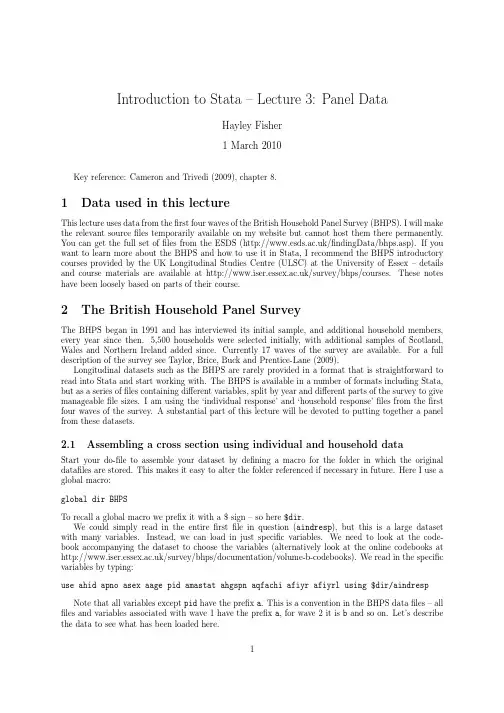
Introduction to Stata–Lecture3:Panel DataHayley Fisher1March2010Key reference:Cameron and Trivedi(2009),chapter8.1Data used in this lectureThis lecture uses data from thefirst four waves of the British Household Panel Survey(BHPS).I will make the relevant sourcefiles temporarily available on my website but cannot host them there permanently. You can get the full set offiles from the ESDS(/findingData/bhps.asp).If you want to learn more about the BHPS and how to use it in Stata,I recommend the BHPS introductory courses provided by the UK Longitudinal Studies Centre(ULSC)at the University of Essex–details and course materials are available at /survey/bhps/courses.These notes have been loosely based on parts of their course.2The British Household Panel SurveyThe BHPS began in1991and has interviewed its initial sample,and additional household members, every year since then.5,500households were selected initially,with additional samples of Scotland, Wales and Northern Ireland added since.Currently17waves of the survey are available.For a full description of the survey see Taylor,Brice,Buck and Prentice-Lane(2009).Longitudinal datasets such as the BHPS are rarely provided in a format that is straightforward to read into Stata and start working with.The BHPS is available in a number of formats including Stata, but as a series offiles containing different variables,split by year and different parts of the survey to give manageablefile sizes.I am using the‘individual response’and‘household response’files from thefirst four waves of the survey.A substantial part of this lecture will be devoted to putting together a panel from these datasets.2.1Assembling a cross section using individual and household dataStart your do-file to assemble your dataset by defining a macro for the folder in which the original datafiles are stored.This makes it easy to alter the folder referenced if necessary in future.Here I use a global macro:global dir BHPSTo recall a global macro we prefix it with a$sign–so here$dir.We could simply read in the entirefirstfile in question(aindresp),but this is a large dataset with many variables.Instead,we can load in just specific variables.We need to look at the code-book accompanying the dataset to choose the variables(alternatively look at the online codebooks at /survey/bhps/documentation/volume-b-codebooks).We read in the specific variables by typing:use ahid apno asex aage pid amastat ahgspn aqfachi afiyr afiyrl using$dir/aindresp Note that all variables except pid have the prefix a.This is a convention in the BHPS datafiles–all files and variables associated with wave1have the prefix a,for wave2it is b and so on.Let’s describe the data to see what has been loaded here..describeContains data from BHPS/aindresp.dtaobs:10,264vars:10size:348,976(99.9%of memory free)----------------------------------------------------------------------------storage display valuevariable name type format label variable label----------------------------------------------------------------------------ahid long%12.0g household identification numberapno byte%8.0g person numberasex byte%8.0g asex sexpid long%12.0g cross-wave person identifieramastat byte%8.0g amastat marital statusahgspn byte%8.0g ahgspn pno of spouse/partneraage byte%8.0g aage age at date of interviewaqfachi byte%8.0g aqfachi highest academic qualificationafiyrl double%10.0g afiyrl annual labour income(1.9.90-1.9.91) afiyr double%10.0g afiyr annual income(1.9.90-1.9.91)----------------------------------------------------------------------------Sorted by:Three variables here are vital for the construction of our panel dataset.ahid is a household identification number which we will use to match data from the householdfile,and apno is a person identification number within a given household.This can be used in combination with,for example,ahgspan to match couples together.pid is a cross-wave person identifier–it has no a prefix since it matches the same variable in all waves–this connects people over time.We also have data on individuals’sex,age, academic qualifications,labour income and total income.We are going to merge in data from the householdfile,so we need to sort the individual data by the household identification number and save it..sort ahid.save aind,replaceThen we load data from the household responsefile–hhresp.dta.use ahid atenure ahhsize ankids afihhyr using$dir/ahhresp.describeContains data from BHPS/ahhresp.dtaobs:5,511vars:5size:104,709(99.9%of memory free)--------------------------------------------------------------------------------------storage display valuevariable name type format label variable label--------------------------------------------------------------------------------------ahid long%12.0g household identification numberahhsize byte%8.0g ahhsize number of persons in householdankids byte%8.0g ankids number of children in householdatenure byte%8.0g atenure housing tenureafihhyr double%10.0g afihhyr annual household income(1.9.90-1.9.91) --------------------------------------------------------------------------------------Sorted by:This gives household ID numbers and data on household size,number of children,how housing is owned and total household income.We see there are5,511observations(as opposed to10,264from the individual dataset).After sorting by household ID we can merge the two datasets together:.merge ahid using aindvariable ahid does not uniquely identify observations in aind.dta.tabulate_merge_merge|Freq.Percent Cum.------------+-----------------------------------1|60.060.063|10,26499.94100.00------------+-----------------------------------Total|10,270100.00.keep if_merge==3(6observations deleted).drop_mergeWe see that there are6observations for which there is no individual data,just household data.I drop these.Another useful command for describing data is codebook.This produces a codebook based on what is in Stata.I have extracted the codebook from my logfile and posted it on my website for reference.Having saved the dataset,we can do some analysis with this cross section.First,recode the missing values.Page A3-14of Taylor et al.(2009)outlines the way missing values are handled in these datafiles –any negative values are in fact missing.We can recode these easily together using mvdecode:.mvdecode_all,mv(-9/-1)atenure:17missing values generatedahgspn:1missing value generatedaqfachi:371missing values generatedafiyrl:352missing values generatedafiyr:352missing values generatedHere_all can be replaced with a list of variables.Having created the necessary variables,simple cross section regressions can be performed.Here I show that the xi prefix can be used to create interaction terms as well as a series of category dummies..generate married=amastat==1.generate age2=aage^2.generate lwages=log(afiyrl)(3937missing values generated).xi:regress lwages aage age2i.asex*i.married ankids i.aqfachi,vce(robust)i.asex_Iasex_1-2(naturally coded;_Iasex_1omitted)i.married_Imarried_0-1(naturally coded;_Imarried_0omitted)i.asex*i.marr~d_IaseXmar_#_#(coded as above)i.aqfachi_Iaqfachi_1-7(naturally coded;_Iaqfachi_1omitted)Linear regression Number of obs=6318F(12,6305)=246.80Prob>F=0.0000R-squared=0.3383Root MSE=.92103------------------------------------------------------------------------------|Robustlwages|Coef.Std.Err.t P>|t|[95%Conf.Interval]-------------+----------------------------------------------------------------aage|.1932962.007231326.730.000.1791205.2074719age2|-.0023262.0000903-25.750.000-.0025033-.0021491 _Iasex_2|-.3133317.0411562-7.610.000-.3940119-.2326515_Imarried_1|.4771106.039076512.210.000.4005075.5537138_IaseXmar_~1|-.7551111.0507519-14.880.000-.854602-.6556201 ankids|-.2082833.0148482-14.030.000-.2373909-.1791756_Iaqfachi_2|-.1241103.0967663-1.280.200-.3138051.0655845_Iaqfachi_3|-.1621818.0964851-1.680.093-.3513254.0269619_Iaqfachi_4|-.3929866.0912033-4.310.000-.5717762-.2141971_Iaqfachi_5|-.5157779.0899938-5.730.000-.6921963-.3393595_Iaqfachi_6|-.5263538.1001379-5.260.000-.7226582-.3300494_Iaqfachi_7|-.7906337.0903131-8.750.000-.967678-.6135893 _cons| 5.916767.167703235.280.000 5.588011 6.245522------------------------------------------------------------------------------Here_Iasex_2gives the effect of being female,_Imarried_1the effect of being married for men,and _IaseXmar_~1the difference in the effect of being married on wages between women and men.2.2Assembling a two wave panelPanel data can be in two formats–long or wide.Wide data stores each variable separately for each wave,so only has one observation for each individual:PID inc1inc2inc3inc41200210220250260066070075032502802002104150190250300Long data stores all observations of a variable,for example income,in the same variable,and has a wave variable and multiple observations for each individual:PID wave inc1120012210132201425021600226602370024750To use the panel data features in Stata you need to have your data in long format.If your data is in wide format you can reconfigure it using the reshape command.To put together a two wave panel in long format we need to extract the same data for wave2–with prefix b.This is done as above:.use bhid bpno bsex bage pid bmastat bhgspn bqfachi bfiyr bfiyrl using$dir/bindresp .sort bhid.save bind,replacefile bind.dta saved.use bhid btenure bhhsize bnkids bfihhyr using$dir/bhhresp.sort bhid.merge bhid using bindvariable bhid does not uniquely identify observations in bind.dta.keep if_merge==3(2observations deleted).drop_merge.save wave2,replacefile wave2.dta savedThere are two other steps to take to both the wave1and wave2datasets constructed here–to add awave variable(just using generate,and to remove the prefix which is done using the command renpfix..generate wave=2.renpfix bTo combine the twofiles we use the append command.1.use wave1.generate wave=1.renpfix a.append using wave2Listing thefirst20observations shows that we now have a long panel dataset with two time periods..sort pid wave.list pid wave hid sex age mastat in1/20,cleanpid wave hid sex age mastat1.1000225111000209female91never ma2.1000449111000381male28never ma3.1000449122000148male29never ma4.1000452111000381male26never ma5.1000452122000148male27never ma6.1000785711000667female57widowed7.1000785722000296female59widowed8.1001457811001221female54married9.1001457822000369female55married10.1001460811001221male57married11.1001460822000369male58married12.1001681311001418male36married13.1001681322000504male37married14.1001684811001418female32married15.1001684822000504female33married16.1001793311001507female49married17.1001793322000717female49married18.1001796811001507male46married19.1001796822000717male46married20.1001905711001604female59never ma2.3Creating a longer panelWhen performing the same operations on several waves of data,we can write do-files more efficientlyusing the foreach and forvalues loop commands.Here I use foreach to perform the same commandsjust substituting the wave prefix each time.2The command to extract all of the data is shown below. foreach w in a b c d{use‘w’hid‘w’pno‘w’sex‘w’age pid‘w’mastat‘w’hgspn‘w’qfachi‘w’fiyr‘w’fiyrl/// using$dir/‘w’indrespsort‘w’hidsave‘w’ind,replace1To create a wide panel we would not remove the prefixes and would use merge to combine the datasets.2The forvalues command would be used when you want to loop over numbers rather than letters or variables.clearuse‘w’hid‘w’tenure‘w’hhsize‘w’nkids‘w’fihhyr using$dir/‘w’hhrespsort‘w’hidmerge‘w’hid using‘w’indkeep if_merge==3drop_mergerenpfix‘w’generate wave=index("abcd","‘w’")save wave‘w’,replace}We start the forvalues comman by defining what should be replaced in each iteration of the loop–in this case w,and giving the list of values to substitute(a,b,c,d for thefirst4waves).We then write out the code substituting‘w’where the prefix would normally be.This reproduces the steps we went through above.The new function used here is index–this returns the position of‘w’in the list abcd and so generates the wave variable.After this code has been run,we can use a similar loop to append thefiles together,and to delete thefiles created in the process:foreach w in a b c{append using wave‘w’}compresssave BHPS,replaceforeach w in a b c d{capture erase wave‘w’.dtacapture erase‘w’ind.dta}Note that compress ensures that the data is being stored as efficiently as possible.Sorting and listing the dataset produced shows:.sort pid wave.list pid wave hid sex age mastat in1/20,cleanpid wave hid sex age mastat1.1000225111000209female91never ma2.1000449111000381male28never ma3.1000449122000148male29never ma4.1000452111000381male26never ma5.1000452122000148male27never ma6.1000452133000192male28never ma7.1000785711000667female57widowed8.1000785722000296female59widowed9.1000785733000257female59widowed10.1001457811001221female54married11.1001457822000369female55married12.1001457833000389female56married13.1001460811001221male57married14.1001460822000369male58married15.1001460833000389male59married16.1001681311001418male36married17.1001681322000504male37married18.1001681333000508male37married19.1001681344000307male39married20.1001684811001418female32marriedThis shows a panel in long format.Note that age mostly increases by one year between waves for each individual(the age variable here is age at interview date which can vary),whilst sex is constant.In order to perform analysis exploiting the panel dimension of the dataset we must declare the data to be a panel–we do this using xtset,and declaring the panel variable(here pid)and time variable(here wave).Note that the panel variable and time variable must together uniquely identify every observation in the dataset..xtset pid wavepanel variable:pid(unbalanced)time variable:wave,1to4,but with gapsdelta:1unitThis shows that we have an unbalanced panel–as seen in the list above we do not have an observation for every person in every time period.Some useful commands to investigate panel data are xtdescribe, xtsum and xttrans:.xtdescribepid:10002251,10004491,...,47737689n=12350wave:1,2,...,4T=4Delta(wave)=1unitSpan(wave)=4periods(pid*wave uniquely identifies each observation)Distribution of T_i:min5%25%50%75%95%max1124444 Freq.Percent Cum.|Pattern---------------------------+---------764361.8961.89|111110098.1770.06| 1...679 5.5075.55|11..596 4.8380.38| (1)527 4.2784.65|111.458 3.7188.36|.111418 3.3891.74|..11290 2.3594.09|.1..197 1.6095.68|..1.533 4.32100.00|(other patterns)---------------------------+---------12350100.00|XXXXxtdescribe gives information about the panel structure–we see that there are12,350individuals and 4time periods,and that62%of people have observations in all four time periods..xtsum sex age nkids fiyr lwages mastatVariable|Mean Std.Dev.Min Max|Observations-----------------+--------------------------------------------+----------------sex overall| 1.531028.499042712|N=39190 between|.499502312|n=12350within|0 1.531028 1.531028|T-bar= 3.17328||age overall|44.0055918.433861597|N=39190between|18.933581596.5|n=12350within| 1.04443532.3389250.33892|T-bar= 3.17328||nkids overall|.5951008.976242609|N=39190 between|.937591509|n=12350within|.2487689-3.154899 3.595101|T-bar= 3.17328||fiyr overall|8939.0168929.790287481.8|N=37455 between|8186.3210160891.5|n=11982within|3631.936-70011.81204307.5|T-bar= 3.12594||lwages overall|8.849195 1.166257-3.32173312.56891|N=23609 between| 1.206297-3.32173311.61299|n=8323within|.4933544 1.25089114.18753|T-bar= 2.8366||mastat overall| 2.497844 2.03162606|N=39185 between| 2.04319706|n=12350within|.5396737-2.002156 6.247844|T-bar= 3.17287xtsum gives summary statistics and shows variation between individuals and within individuals–so we see that sex does not vary within individuals,and that log wages vary more between individuals than within individuals.We also see the total number of observations(N),number of individuals with observations(n)and average number of time periods for each individual..xttrans married,freq|Married=1Married=1|01|Total-----------+----------------------+----------0|10,669492|11,161|95.59 4.41|100.00-----------+----------------------+----------1|36715,312|15,679| 2.3497.66|100.00-----------+----------------------+----------Total|11,03615,804|26,840|41.1258.88|100.00xttrans gives an indication of whether there are transitions between groups for categorical variables–for example,we see here that96%of unmarried individuals remain unmarried in the next period,and 98%of married individuals remain married in the next period.3Regression using panel dataHaving set up our dataset we can perform some regressions.As previously,I use a local macro to store my list of independent variables:local xlist"age age2i.sex*i.married nkids i.qfachi"We can estimate a pooled OLS regression using the regress command seen in the last lecture.We should use robust standard errors clustered by individual..xi:regress lwages‘xlist’,vce(cluster pid)i.sex_Isex_1-2(naturally coded;_Isex_1omitted)i.married_Imarried_0-1(naturally coded;_Imarried_0omitted)i.sex*i.married_IsexXmar_#_#(coded as above)i.qfachi_Iqfachi_1-7(naturally coded;_Iqfachi_1omitted)Linear regression Number of obs=23520F(12,8285)=409.27Prob>F=0.0000R-squared=0.3092Root MSE=.96854(Std.Err.adjusted for8286clusters in pid)------------------------------------------------------------------------------|Robustlwages|Coef.Std.Err.t P>|t|[95%Conf.Interval]-------------+----------------------------------------------------------------age|.1890312.005557434.010.000.1781373.1999251age2|-.0022714.0000708-32.100.000-.0024101-.0021327 _Isex_2|-.3258962.0300076-10.860.000-.3847186-.2670737_Imarried_1|.488806.028615817.080.000.4327118.5449002_IsexXmar_~1|-.654709.0376179-17.400.000-.7284494-.5809685 nkids|-.2203951.0115555-19.070.000-.2430467-.1977435 _Iqfachi_2|-.1272603.077578-1.640.101-.2793325.024812_Iqfachi_3|-.1781531.0785097-2.270.023-.3320517-.0242544_Iqfachi_4|-.4158935.0734584-5.660.000-.5598903-.2718966_Iqfachi_5|-.5313831.0726375-7.320.000-.6737708-.3889953_Iqfachi_6|-.617404.080617-7.660.000-.7754335-.4593746_Iqfachi_7|-.8375914.073551-11.390.000-.9817697-.693413 _cons| 6.046451.129803846.580.000 5.792003 6.300899------------------------------------------------------------------------------Fixed and random effects regressions are both carried out using the xtreg command.In both cases we should again get cluster robust standard errors.The default is for Stata to estimate random effects when xtreg is used–you must specify the option“fe”to getfixed effects:.xi:xtreg lwages‘xlist’,fe vce(cluster pid)i.sex_Isex_1-2(naturally coded;_Isex_1omitted)i.married_Imarried_0-1(naturally coded;_Imarried_0omitted)i.sex*i.married_IsexXmar_#_#(coded as above)i.qfachi_Iqfachi_1-7(naturally coded;_Iqfachi_1omitted)Fixed-effects(within)regression Number of obs=23520Group variable:pid Number of groups=8286R-sq:within=0.0451Obs per group:min=1 between=0.1672avg= 2.8overall=0.1293max=4F(11,8285)=38.35corr(u_i,Xb)=-0.3782Prob>F=0.0000(Std.Err.adjusted for8286clusters in pid)------------------------------------------------------------------------------|Robustlwages|Coef.Std.Err.t P>|t|[95%Conf.Interval]-------------+----------------------------------------------------------------age|.2902458.017377516.700.000.2561815.3243102age2|-.0030951.0002108-14.680.000-.0035083-.0026819 _Isex_2|(dropped)_Imarried_1|.0473639.0421936 1.120.262-.0353461.1300739_IsexXmar_~1|-.0574721.0682978-0.840.400-.1913529.0764086 nkids|-.1347352.0193899-6.950.000-.1727443-.0967261 _Iqfachi_2|.0239754.27867750.090.931-.5223023.5702531_Iqfachi_3|-.2838254.2629136-1.080.280-.7992019.231551_Iqfachi_4|-.1524719.2703457-0.560.573-.6824172.3774734_Iqfachi_5|-.4847609.2739852-1.770.077-1.021841.0523187_Iqfachi_6|-.4576768.3040223-1.510.132-1.053637.138283_Iqfachi_7|-.3651604.3077017-1.190.235-.9683329.238012 _cons| 3.198992.444527.200.000 2.327621 4.070362-------------+----------------------------------------------------------------sigma_u| 1.1636036sigma_e|.59940523rho|.79029066(fraction of variance due to u_i)------------------------------------------------------------------------------Here sex is dropped–this is because it is invariant over time.The lack of variance in qualifications and marital status explains the imprecise coefficient estimates here..xi:xtreg lwages‘xlist’,re vce(cluster pid)i.sex_Isex_1-2(naturally coded;_Isex_1omitted)i.married_Imarried_0-1(naturally coded;_Imarried_0omitted)i.sex*i.married_IsexXmar_#_#(coded as above)i.qfachi_Iqfachi_1-7(naturally coded;_Iqfachi_1omitted)Random-effects GLS regression Number of obs=23520Group variable:pid Number of groups=8286R-sq:within=0.0341Obs per group:min=1 between=0.3457avg= 2.8overall=0.3053max=4 Random effects u_i~Gaussian Wald chi2(12)=4356.47corr(u_i,X)=0(assumed)Prob>chi2=0.0000(Std.Err.adjusted for8286clusters in pid)------------------------------------------------------------------------------|Robustlwages|Coef.Std.Err.z P>|z|[95%Conf.Interval]-------------+----------------------------------------------------------------age|.2133805.005807336.740.000.2019984.2247626age2|-.0025222.0000737-34.220.000-.0026667-.0023778 _Isex_2|-.4601064.0312502-14.720.000-.5213557-.3988571_Imarried_1|.341099.027577812.370.000.2870475.3951504_IsexXmar_~1|-.4701444.0385164-12.210.000-.5456351-.3946536 nkids|-.201973.0116565-17.330.000-.2248194-.1791267 _Iqfachi_2|-.0940869.0991879-0.950.343-.2884916.1003178_Iqfachi_3|-.1635236.0960624-1.700.089-.3518024.0247552_Iqfachi_4|-.3019628.0911546-3.310.001-.4806225-.1233031_Iqfachi_5|-.4841929.0903848-5.360.000-.6613438-.3070421_Iqfachi_6|-.524829.0975616-5.380.000-.7160463-.3336117_Iqfachi_7|-.785563.0915491-8.580.000-.9649959-.6061301 _cons| 5.485352.146495337.440.000 5.198227 5.772478-------------+----------------------------------------------------------------sigma_u|.87706892sigma_e|.59940523rho|.68163491(fraction of variance due to u_i)------------------------------------------------------------------------------Stata reports the standard deviations of the error components estimated in sigma_u and sigma_e.We also see different R2statistics for within and between variation.These can be tabulated if the estimates have been stored..esttab POLS FE RE,b se stats(r2r2_o r2_b r2_w)------------------------------------------------------------(1)(2)(3)lwages lwages lwages------------------------------------------------------------age0.189***0.290***0.213***(0.00556)(0.0174)(0.00581)age2-0.00227***-0.00310***-0.00252***(0.0000708)(0.000211)(0.0000737)_Isex_2-0.326***0-0.460***(0.0300)(0)(0.0313)_Imarried_10.489***0.04740.341***(0.0286)(0.0422)(0.0276)_IsexXmar_~1-0.655***-0.0575-0.470***(0.0376)(0.0683)(0.0385)nkids-0.220***-0.135***-0.202***(0.0116)(0.0194)(0.0117)_Iqfachi_2-0.1270.0240-0.0941(0.0776)(0.279)(0.0992)_Iqfachi_3-0.178*-0.284-0.164(0.0785)(0.263)(0.0961)_Iqfachi_4-0.416***-0.152-0.302***(0.0735)(0.270)(0.0912)_Iqfachi_5-0.531***-0.485-0.484***(0.0726)(0.274)(0.0904)_Iqfachi_6-0.617***-0.458-0.525***(0.0806)(0.304)(0.0976)_Iqfachi_7-0.838***-0.365-0.786***(0.0736)(0.308)(0.0915)_cons 6.046*** 3.199*** 5.485***(0.130)(0.445)(0.146)------------------------------------------------------------r20.3090.0451r2_o0.1290.305r2_b0.1670.346r2_w0.04510.0341------------------------------------------------------------Standard errors in parentheses*p<0.05,**p<0.01,***p<0.001Estimation can also be easily implemented infirst differences using the regress command and dif-ference operator“D.”.We do not need to generate variables infirst differences.The option noconstant is used so that Stata does not add a constant term(which would be differenced out).For example:.regress D.(lwage age age2female married nkids),vce(cluster pid)noconstantLinear regression Number of obs=14667F(4,6146)=65.00Prob>F=0.0000R-squared=0.0208Root MSE=.73681(Std.Err.adjusted for6147clusters in pid)------------------------------------------------------------------------------|RobustD.lwages|Coef.Std.Err.t P>|t|[95%Conf.Interval]-------------+----------------------------------------------------------------age|D1.|.3179554.021196115.000.000.2764036.3595071age2|D1.|-.0034294.0002499-13.720.000-.0039192-.0029395 female|D1.|(dropped)married|D1.|.0144043.03906050.370.712-.062168.0909767 nkids|D1.|-.0957519.0221907-4.310.000-.1392534-.0522504------------------------------------------------------------------------------3.1Hausman testStata can easily perform a Hausman test–that is,a test of whether the individual effects are random. The null hypothesis is that bothfixed and random effects are consistent,the alternative hypothesis is that random effects is not consistent.We mustfirst estimate thefixed and random effects models–and without robust standard errors.Then,the Hausman test is conducted using the hausman command..quietly xi:xtreg lwages‘xlist’,fe.estimates store FE1.quietly xi:xtreg lwages‘xlist’,re.estimates store RE1.hausman FE1RE1,sigmamore----Coefficients----|(b)(B)(b-B)sqrt(diag(V_b-V_B))|FE1RE1Difference S.E.-------------+----------------------------------------------------------------age|.2902458.2133805.0768653.0125061age2|-.0030951-.0025222-.0005729.0001535_Imarried_1|.0473639.341099-.293735.0336022_IsexXmar_~1|-.0574721-.4701444.4126723.0470245nkids|-.1347352-.201973.0672378.0120169_Iqfachi_2|.0239754-.0940869.1180623.1387245_Iqfachi_3|-.2838254-.1635236-.1203018.1676963_Iqfachi_4|-.1524719-.3019628.1494909.1630687_Iqfachi_5|-.4847609-.4841929-.000568.1697845_Iqfachi_6|-.4576768-.524829.0671522.2006431_Iqfachi_7|-.3651604-.785563.4204026.1869317------------------------------------------------------------------------------b=consistent under Ho and Ha;obtained from xtreg B=inconsistent under Ha,efficient under Ho;obtained from xtreg Test:Ho:difference in coefficients not systematicchi2(11)=(b-B)’[(V_b-V_B)^(-1)](b-B)=238.04Prob>chi2=0.0000Cameron and Trivedi(2009)recommend using the sigmamore option.Here we see the null hypothesis is clearly rejected with a p-value of0.0000so the random effects estimates are not consistent.4Creating variables to identify changes in variablesWe may wish to create a variable which records whether a certain status has changed.For example, whether marital status has changed.Once data is declared to be a panel this is straightforward.Let’s first recode mastat so that it has just three categories:recode mastat(0=.)(1/2=1)(3/5=2)(6=3),generate(ma)Then tofind changes we generate a new variable which incorporates the lagged value and current value of ma:generate mach=(10*L.ma)+maHaving labelled the values we have a useful marital change variable.So we can see that there are352 instances of individuals going from never having been married to having a partner in this sample..tabulate machmarital change|Freq.Percent Cum.-----------------------------+-----------------------------------stayed in couple|16,84963.9463.94partnership ended|360 1.3765.30partnered->never married!|1130.4365.73ex-partner->partnership|1800.6866.41stayed ex-partner|3,62213.7480.16never married->partnership|352 1.3481.49never married->ex-partner|140.0581.55stayed never married|4,86318.45100.00-----------------------------+-----------------------------------Total|26,353100.00ReferencesCameron,A.Colin and Pravin K.Trivedi,Microeconometrics Using Stata,Texas:Stata Press, 2009.Taylor,Marcia Freed,John Brice,Nick Buck,and Elaine Prentice-Lane,“British Household Panel Survey User Manual Volume A:Introduction,Technical Report and Appendices,”ISER, University of Essex,Colchester2009.。

Stata统计分析与建模入门教学第一章:Stata的介绍和基本操作Stata是一款专业的统计分析软件,被广泛应用于学术研究、政府机构和企业中。
本章将介绍Stata的基本功能和操作界面,包括数据导入、数据管理和数据处理等内容。
学习者可以通过本章的教学示例,快速熟悉Stata的基本操作,并掌握如何在Stata中进行数据的读取和保存。
第二章:数据清理和准备本章重点介绍如何对原始数据进行清洗和准备,以便于后续的统计分析和建模。
内容包括缺失值处理、异常值处理、数据变量的重编码和转换等。
通过学习本章,学习者将掌握如何使用Stata 来处理常见的数据质量问题,保证数据的准确性和完整性。
第三章:描述性统计和数据可视化描述性统计和数据可视化是统计分析的常用方法,可以帮助研究者对数据进行初步的了解和分析。
本章将介绍在Stata中如何计算和呈现数据的描述统计量,包括均值、标准差、百分位数等指标,并且教学者将指导学生使用Stata绘制直方图、散点图和箱线图等数据可视化图形。
第四章:假设检验和置信区间假设检验和置信区间是统计学中重要的概念和方法,可以用于推断总体参数,并进行统计显著性检验。
本章将介绍如何在Stata中进行常见的假设检验,比如 t检验、方差分析和卡方检验等,并演示如何计算和解释置信区间。
学习者通过本章的学习,将能够掌握在Stata中进行假设检验的方法和技巧。
第五章:线性回归分析线性回归分析是最常用的统计建模方法之一,可以用于探究自变量与因变量之间的关系。
本章将介绍在Stata中进行线性回归分析的步骤和技巧,包括模型的建立、参数估计和统计推断等内容。
学习者将通过本章学会如何使用Stata进行简单线性回归和多元线性回归分析,并能够对回归模型进行解释和评估。
第六章:非线性回归分析非线性回归分析是一类应用广泛的统计建模方法,用于描述自变量和因变量之间的非线性关系。
本章将介绍在Stata中进行非线性回归分析的方法和技巧,包括多项式回归、对数回归和指数回归等内容。
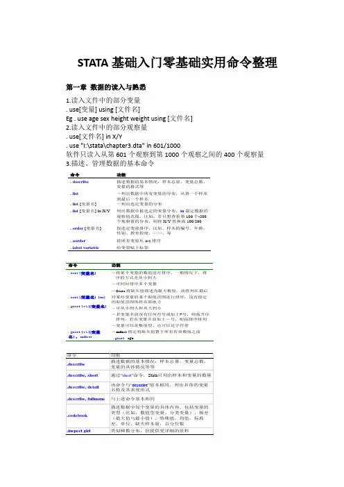
STATA基础入门零基础实用命令整理第一章数据的读入与熟悉1.读入文件中的部分变量. use[变量] using [文件名]Eg . use age sex height weight using [文件名]2.读入文件中的部分观察量. use[文件名] in X/Y. use "I:\stata\chapter3.dta" in 601/1000软件只读入从第601个观察到第1000个观察之间的400个观察量3.描述、管理数据的基本命令命令功能. describe描述数据的基本情况:样本总量、变量总数、变量的格式等. list. list [变量名]-列出数据中所有变量的分布,从第一个样本到最后一个样本-列出选定变量的分布. list [变量名] in X/Y 列出数据中被选定的变量分布。
in限定数据的观察值范围。
比如,若只想查看第100个-200个观察值的分布,则将X/Y替换成100/200. order [变量名]按选定变量排序。
比如,样本的编号、年龄、性别、教育程度,……,等. aorder 将所有变量从 a-z 排序. label variable给变量贴上标签命令功能. sort [变量名] -将某个变量的数值进行排序。
一般情况下,排序的方式是从小到大-可同时排序多个变量-Stata将缺失值描述为最大数值,故排列在最后. sort [变量名] [in] 对某些变量的某个取值范围进行排序;没有指定的取值范围保持在原地方. gsort [+|-][变量名] -可从小到大和从大到小-若变量名前没有任何符号或加上+号,则按升序排列;若在变量名前加上-号,则按降序排列-变量可以是数值型、也可以是字符型. gsort [+|-][变量名] ,mfirst -mfirst指定将缺失值置于所有有效数值之前. gsort -age第二章变量的生成与处理1.离散和连续测量离散方式(discrete measure):由定性测量和定序测量组成;适用于低层次数据连续方式(continuous measure):由定距测量和定比测量组成。
stata学习-基础篇3View中红⾊为字符型(str)⿊⾊为数字型字符型:加引号“”;数字型:直接写= 赋值== 等于年龄的计算:检查⽇期-出⽣⽇期gen age=(deb-dob)/365.25order A ,a (B) /将变量A放在变量B后merge /合并merge 1:m varname using C:\.......\dataset namemerge m:m varname using C:\.......\dataset namemerge m:1 varname using C:\.......\dataset nameset more off /直接跳⾏⾄列表最后(结果框的more不⽤⼀直点了)log⽤法:如果你想将 Stata 的屏幕输出窗⼝中的内容保存下来,需要⽤ Log ⽇志⽂件记录。
使⽤下⾯语句. log using D:\Stata\d1.log表⽰新建在 D 盘的 Stata ⽂件下的 d1⽇志⽂件 1。
这⾥的 using 不仅表⽰新建,也可以表⽰打开⽇志⽂件。
打开有下⾯两种情况:. log using D:\Stata\d1.log,append. log using D:\Stata\d1.log,replace记录的过程中若需要暂停 (⽐如要试⽤⼀个新命令,检验其语句正确与否 ) ,则有:. log off. log on最后,结束⽇志记录:. log close修改label名:label variable hbp "high blood pressure" /和rename差不多关系运算符:== 等于!=不等于> ⼤于< ⼩于>=⼤于等于<= ⼩于等于逻辑运算符:& 和| 或!或者⽤~ 表⽰否order od, before(os) / 将od变量置于os前⾯order od, last / 将od变量置于最后⾯order id age sex od os / 将变量按照 id age sex od os 排列长宽数据转换格式:reshape long stubnames, i(varlist) [options]reshape wide stubnames, i(varlist) [options]long表⽰将宽数据转化为长数据,wide表⽰将长数据转化成宽数据,stubnames表⽰需要转化的变量的名称前缀,i(varlist)表⽰识别变量。
Stata统计分析软件入门指导第一章:Stata软件介绍Stata统计分析软件是一款功能强大的数据分析工具,广泛应用于社会科学、经济学、统计学等研究领域。
本章将介绍Stata 软件的基本特点、应用领域以及优势,并给出软件安装与启动的步骤。
第二章:数据准备数据准备是进行数据分析的前提,本章将介绍如何导入数据到Stata软件中,并对常见的数据格式进行转换。
同时,还将介绍数据清洗和变量定义等操作,以提高数据的质量和可用性。
第三章:数据描述与探索数据描述和探索是数据分析的基础工作,本章将介绍Stata 中常用的数据描述统计方法,包括均值、中位数、标准差等常见统计指标的计算。
此外,还将介绍绘制直方图、散点图和箱线图等图形来展示数据分布和变量之间的关系。
第四章:基本统计分析基本统计分析是Stata软件的核心功能之一,本章将详细介绍Stata中的统计分析方法,包括描述统计、t检验、方差分析、相关分析等常见方法。
同时,还将介绍如何进行变量转换和生成新变量,以应对实际问题中的需求。
第五章:回归分析回归分析是一种常用的统计方法,可用于探索变量之间的关系、预测未来值、解释数据的变异等。
本章将介绍Stata中的线性回归、多元回归和逻辑回归等方法,并详细解释结果的解读与应用。
第六章:高级统计分析高级统计分析方法可以进一步深入研究数据,发现更深层次的信息。
本章将介绍Stata中的时间序列分析、生存分析和聚类分析等方法,并结合实例说明如何应用这些方法解决实际问题。
第七章:数据可视化数据可视化是将数据以图形的方式展示,有助于更好地理解数据和发现规律。
本章将介绍Stata中绘制折线图、柱状图、饼图、雷达图等常用图形的方法,并结合实例演示如何选择合适的图形来表达数据。
第八章:扩展功能与编程Stata软件提供了许多扩展功能和编程方法,可以增强数据分析的效率和灵活性。
本章将介绍Stata中的扩展命令和程序化编程,并演示如何自定义命令和自动化分析过程,以提高工作效率。
STATA基本操作入门1.数据导入在STATA中,可以导入多种格式的数据文件,如Excel、CSV和文本文件。
最常用的命令是"import excel"和"import delimited"。
例如,要导入名为"data.xlsx"的Excel文件,可以使用以下命令:```import excel using "data.xlsx", sheet("Sheet1") firstrow clear```这里,"using"指定了文件路径和文件名,"sheet"指定了工作表名称(如果有多个工作表),"firstrow"表示第一行是变量名。
2.数据清洗在导入数据后,通常需要进行数据清洗,包括处理缺失值、异常值和重复值等。
STATA提供了一些常用的命令来处理这些问题。
- 缺失值处理:使用"drop"命令删除带有缺失值的观测值,使用"egen"命令创建新变量来表示缺失值。
- 异常值处理:可以使用描述性统计命令(如"summarize")来查找异常值,并使用"drop"命令删除异常值所对应的观测值。
- 重复值处理:使用"deduplicate"命令删除重复的观测值,或使用"egen"命令创建新变量来表示重复值。
3.变量操作在STATA中,可以对变量进行各种操作,如创建变量、重命名变量、计算变量和合并变量等。
- 创建变量:可以使用"generate"命令创建新变量,并赋予其数值或字符值。
- 重命名变量:使用"rename"命令将变量重命名为新的名称。
- 计算变量:使用"egen"命令计算新变量,例如,可以使用"egen mean_var = mean(var)"计算变量"var"的均值,并将结果赋值给新的变量"mean_var"。
学习如何使用Stata进行数据分析Stata是一种功能强大的统计分析软件,广泛应用于社会科学、医学研究、经济学等领域。
它提供了各种数据处理、统计分析和图形展示的功能,可帮助研究人员深入挖掘数据背后的信息。
本文将介绍Stata的基本功能和使用方法,并通过几个具体的实例说明如何进行数据分析。
第一章:Stata的安装与介绍首先,我们需要下载并安装Stata软件。
Stata有不同的版本,根据自己的需求选择合适的版本进行下载。
安装完成后,打开Stata,我们将看到一个交互式界面,可以在其中输入命令进行数据处理和统计分析。
第二章:数据导入和管理在使用Stata进行数据分析之前,首先需要导入数据。
Stata支持多种数据格式,包括Excel、CSV、SPSS等。
通过"import"命令可以将这些数据导入到Stata中,并且根据需要进行数据管理,如删除变量、修改变量标签等。
此外,还可以使用"describe"命令查看数据集的基本信息。
第三章:数据清洗和整理在数据分析过程中,数据质量的好坏直接影响结果的可靠性。
Stata提供了一些命令和工具,帮助我们对数据进行清洗和整理,如去除异常值、填充缺失值、变量重编码等。
在此过程中,我们还可以使用一些函数和运算符对数据进行简单的计算和转换。
第四章:描述性统计分析描述性统计分析是数据分析的第一步,用于了解数据的基本情况。
Stata提供了丰富的命令和函数,可计算数据的均值、标准差、中位数、百分位数等统计量,并生成频数表和基本图表。
通过这些统计量和图表,我们可以对数据集的整体情况有一个直观的认识。
第五章:统计推断和假设检验统计推断和假设检验是数据分析的核心内容。
Stata提供了一系列命令和工具,可进行参数估计、假设检验和置信区间估计等统计推断动作。
比如,可以使用"regress"命令进行线性回归分析,使用"ttest"命令进行均值差异显著性检验等。
3数据数据文件是一个矩形的矩阵,这个矩阵的每一行都代表或对应着一个“观测单位”(比如是一个人,一个村或一个地区等等),矩阵的每一列都代表或对应着一个“变量”(比如年龄,身高、体重,月工资收入等等)。
因此,数据文件矩阵中的每一个元素(case)都代表或对应着某一个“观测单位”(如张三、李四,A 厂、B厂)中的某一个“变量”(比如年龄、体重,月收入等等)的变量值或观察值。
3.1 打开示例数据和网络数据:use3.1.1 示例数据示例数据为STATA帮助文件中所用的数据,其后辍名为.dta,如果在STATA 软件当前路径下,直接用use命令即可打开,如果不在当前路径下,则可以使用sysuse命令打开。
. use auto,clear //打开汽车数据auto.dta. cd d:/ //改变路径到d:/. use auto, clearfile auto.dta not found //系统提示无法找到文件,因为auto.dta不在d:/ r(601);3.1.2 从网络获取数据上述示例数据可能没有全部下载安装于你的电脑中,因此简单地使用use和sysuse命令时,可能出现错误,如. use nlswork, clearfile nlswork.dta not found此时,如果确定该数据为示例数据,可以直接通过网络获取,其命令为:. use /data/r9/nlswork //从网站获取数据,或者. webuse nlswork, clear //与前一命令等价,从STATA官方数据库获取数据webuse只能从/data这一路径获取数据,如果不是该网站的数据,webuse失效,只能把网站地址完全写出来。
使用该命令时必须确保网络连接正常.另一个网络数据较多的地方是波士登大学的数据中心,我们所用的《计量经济学导论》一书中所使用的全部数据都可以通过该数据中心获得。
比如. use /ec-p/data/wooldridge/CEOSAL1即打开教材中例2.3中所使用的CEO数据。
use命令只能打开后辍名为“*.dta”格式的数据,.dta格式以外的数据,STATA 不能直接读取,需要从外部读入,最简单而直接的办法是复制和粘贴,但有时没有其他软件,比如有SAS格式或SPSS格式的数据,但没有SAS软件和SPSS 软件,此时需要用STATA提供的其他命令或者使用transfer数据格式转化软件。
在讨论其他输入或导入数据的方法之前,我们先来学习一点数据类型的知识。
3.2数据类型STATA通常把变量划分为三类:分别是数值型,字符型和日期型3.2.1数值变量:用0、1、2…9及+、–(正负号)与小数点“(.)”来表示。
在输入数据时,逗号不能被识别,如1,024应该直接写成1024.其他示例5-55.25.2e+35.2e-2后面两个数据为科学计数法的数据,分别表示5200和0.052.其中的e相当于10,因此5.2e+3的意思是:5.2*103=5200数值型变量按其精度区分,又有五种类型,分别是:存贮类型最小最大0-领域字节--------------------------------------------------------------------- byte -127 100 +/-1 1 int -32,767 32,740 +/-1 2 long -2,147,483,647 2,147,483,620 +/-1 4float -1.70141173319*10^38 1.70141173319*10^36 +/-10^-36 4 double -8.9884656743*10^307 8.9884656743*10^307 +/-10^-323 8 当运算精度要求很高的时候,需要将变量设置成浮点型和双精度型。
注意1和 1.0000的精度是不同的,前者在(0.5,1.5)区间内近似,而后者在(0.99995,1.00005)区间内近似。
若多次运算反复取四舍五入,精度较低时将使计算误差迅速变大,然而,精度高时占用的内存资源较多。
下面的命令有助于理解变量存贮类型变换。
clearset obs 1obs was 0, now 1 //提示信息说,之前系统中没有观察单位,现在有了一个gen a=1 //生成一个新变量a,令a取值为1d /*d为describ命令的略写,describ命令显示数据集的属性信息,注意观察显示结果中,a的storage type为float型,浮点型为默认类型*/Contains dataobs: 1 (观察值个数)vars: 1 (变量个数)size: 8 (99.9% of memory free)(内存空间大小)storage display valuevariable name type format label variable labela float %9.0gSorted by: (按什么分类)Note: dataset has changed since last saved(注释)compress //在不损害信息的基础上压缩,使数据占用空间尽可能小a was float, now byte//a由浮点型变为了字节型d // 注意a的storage type现在为byte型replace a=101 /* 注意a的storage type现在自动升为int型,因为byte最大只能为100*/a was byte now int(1 real change made)replace a=100compressd//重新变回到byte型replace a=32741//直接变到long型,因为int型最大只能到32740gen double b=1 //直接生成双精度变量brecast double a//将a变成双精度变量bd//注意到a和b均为双精度型3.2.2字符串变量:字符变量通常是一些身份信息,如姓名,地名。
另外,分类形迹也可以用字符变量来表示,如性别分为“男”和“女”。
字符串变量由字母或一些特殊的符号组成的(如地名〈籍贯〉变量,迁出地,住址,职业等等)。
字符串变量也可以由数字来组成,但数字在这里仅代表一些符号而不再是数字。
字符串变量通常以引号“”注标,而且引号一般不被试同为字符的一部分。
注意这里的引号必须是英文输入状态下的引号。
字符串最多可以达244个字符。
一般用str#来表示字符的多少,如str20表示将有20个字符。
一般三个中文字的姓名需要6个字符。
字符型示例“String”“string”” string””string ”””//特殊字符串,表示空字符,缺失值。
””//注意与空字符串的区别,含有一个空格”125.27”//”125.27”由于有双引号,将被视同为字符而非数值。
“$2,343.68”“I love you”“旺材是条狗”注意前四个字符串均不相同,大小写是不一样的,有无空格及空格的位置不同,都表示不同的字符串。
对于”125.27”这样的数值型的字符串,可以用real()函数或者destring命令转化成数值型变量。
具体操作见3.3.1。
3.2.3日期型变量在STATA中,1960年1月1日被认为是第0天,因此1959年12月31日为第-1天,2001年1月25日为15000天。
对日期型变量的讨论将在后面的时间序列分析部分。
1999 12 10jan/10/200110jan2001...-15,000 --- 01dec1918-31 ---01dec1959...-1 --- 31dec19590 --- 01jan19601 ---- 02jan1960...31 ---- 01feb1960...15,000 ---- 25jan20013.2.4缺失值没有意义的计算结果显示为”.”如将一个字符型数据和一个数据值型数据相加没有意义,结果输出为“.”. display 2/0另一种情况是,数据中含有缺失值,STATA默认的缺失值也用“.”来表示。
在有些数据文件中,缺失值不是用“.”或者空来表示的,而是用-9996等来表示,如果要将其全部替换为“.”,或者反之,将“.”替换为-9996,命令为:. mvencode age,mv(-9996). mvdecode age,mv(-9996)3.3数据类型转化任务:将destring1, destring2和tostring中的数据类型进行相互转化*3.3.1字符型转化成数值型:destring*destring1数据中的数据全为字符型,转换为数值型webuse destring1, cleardes /*注意到所有的变量存贮类型(storage type)均为字符型str#,其中#号表示字符串长度*/Contains data from /data/r9/destring1.dta obs: 10vars: 5 3 Mar 2005 10:15size: 240 (99.9% of memory free)storage display valuevariable name type format label variable labelid str3 %9snum str3 %9scode str4 %9stotal str5 %9sincome str5 %9ssum //因为所有变量为字符型,所以不能进行数值计算gen nincom=incom+10 //因字符不能进行四则运算,不能进行加法运算*type mismatch //系统提示类型不匹配,因为income为字符型,10为数值型destring, replace //全部转换为数值型,replace表示将原来的变量(值)更新sum //注意到转换为数值型后,可以求五数概略了gen nincom=income*1.3 //转换后,可以运算,工资终于涨了30%!list nincom income*----------------将字符型数据转换为数值型数据:去掉字符间的空格------------*destring2数据集中的data变量为字符型,且年月日间有空格,转移为数据型webuse destring2, cleardes //注意到所有的变量均为字符型strlist date //注意到date年月日之间均有空格date------------1. 1999 12 102. 2000 07 083. 1997 03 024. 1999 09 00destring date, replace//想把date转换成数值型,但失败了,系统提示说*date contains non-numeric characters; no replace /*由于含有非数值型字符(即空格),因此没有更新,也即转换命令没有执行。