partial-differential-equation-toolbox[1]

基于Matlab的四层椭圆头模型EIT正向计算研究李英一;刘文礼;陶佰睿;郭福三【摘要】目的:探寻一种可用于头部EIT(电阻抗成像技术)正问题相对精确并且实现简单的求解方法,使得逆问题的结果能够更加接近人体头部的真实阻抗分布.方法:利用Matlab构建一种比传统圆形或同心圆更加符合人脑形状的二维四层椭圆头模型结构,并对其进行剖分和正向仿真计算.结果:实现了模型的建立、剖分、偏微分方程的求解以及解的可视化.结论:与使用其它编程语言实现正向计算相比,这一方法更加直观,程序调试以及修改都更加容易;构建的模型更加接近人头部的真实结构,为逆问题的精确求解奠定了基础.【期刊名称】《齐齐哈尔大学学报（自然科学版）》【年(卷),期】2015(031)006【总页数】3页(P9-11)【关键词】四层椭圆头模型;电阻抗成像技术;正问题;仿真计算【作者】李英一;刘文礼;陶佰睿;郭福三【作者单位】齐齐哈尔大学通信与电子工程学院,黑龙江齐齐哈尔161006;齐齐哈尔大学通信与电子工程学院,黑龙江齐齐哈尔161006;齐齐哈尔大学通信与电子工程学院,黑龙江齐齐哈尔161006;齐齐哈尔大学通信与电子工程学院,黑龙江齐齐哈尔161006【正文语种】中文【中图分类】TP391.41Matlab是一种以矩阵为基本数据元素的数值计算工具，它既有高效的科学计算功能，又有强大的图形处理功能，并且其一个重要特色就是拥有一套程序扩展系统和被称之为工具箱的特殊应用子程序。

Matlab提供了一个图形用户界面（GUI）的偏微分方程数值求解工具Partial Differential Equation TOOLBOX［1］。

利用该工具，可以交互式地实现偏微分方程数学模型的几何模型建立、边界条件设定、三角形网格剖分和加密，以及偏微分方程类型设置、参数给定、方程求解和结果图形显示。

它包括了数值求解的前处理、计算和后处理等一套完整的程序，可以直观、快速、准确、形象地实现偏微分方程的数值求解。

（整理）matlab部分工具箱.1)通讯工具箱(Communication Toolbox)。

令提供100多个函数和150多个SIMULINK模块用于通讯系统的仿真和分析——信号编码——调制解调——滤波器和均衡器设计——通道模型——同步可由结构图直接生成可应用的C语言源代码。

2)控制系统工具箱(Control System Toolbox)。

鲁连续系统设计和离散系统设计* 状态空间和传递函数* 模型转换* 频域响应：Bode图、Nyquist图、Nichols图* 时域响应：冲击响应、阶跃响应、斜波响应等* 根轨迹、极点配置、LQG3)财政金融工具箱(FinancialTooLbox)。

* 成本、利润分析，市场灵敏度分析* 业务量分析及优化* 偏差分析* 资金流量估算* 财务报表4)频率域系统辨识工具箱(Frequency Domain System ldentification Toolbox* 辨识具有未知延迟的连续和离散系统* 计算幅值／相位、零点／极点的置信区间* 设计周期激励信号、最小峰值、最优能量诺等5)模糊逻辑工具箱(Fuzzy Logic Toolbox)。

* 友好的交互设计界面* 自适应神经—模糊学习、聚类以及Sugeno推理* 支持SIMULINK动态仿真* 可生成C语言源代码用于实时应用(6)高阶谱分析工具箱(Higher—Order SpectralAnalysis Toolbox * 高阶谱估计* 信号中非线性特征的检测和刻画* 延时估计* 幅值和相位重构* 阵列信号处理* 谐波重构(7)图像处理工具箱(Image Processing T oolbox)。

* 二维滤波器设计和滤波* 图像恢复增强* 色彩、集合及形态操作* 二维变换* 图像分析和统计(8)线性矩阵不等式控制工具箱(LMI Control Toolbox)。

* LMI的基本用途* 基于GUI的LMI编辑器* LMI问题的有效解法* LMI问题解决方案(9)模型预测控制工具箱(ModelPredictive Control Toolbox* 建模、辨识及验证* 支持MISO模型和MIMO模型* 阶跃响应和状态空间模型(10)u分析与综合工具箱(u-Analysis and Synthesis Toolbox)* u分析与综合* H2和H无穷大最优综合* 模型降阶* 连续和离散系统* u分析与综合理论(11)神经网络工具箱(Neursl Network T oolbox)。

节点的广义薄膜位移 u
应用数值积分即可求得薄膜所围成得体积
其二倍即得扭
转惯性矩 I t 计算式 7 时采用二重积分的梯形公式 即计算斜顶三棱柱的体积 如式 8 这种方法虽精度较低 但编程简单
In =
1 n ∑ [(u1i + u2i + u3i )Ai ] 3 i =1
薄膜比拟中 第 i 三角形单元角点的薄膜竖向位移
剖分 T 型钢扭转惯性矩的二倍总是略小于相应的 H 型钢计
4
结论
本文针对国标 GB/T11263-1998 提供的基本数据以及山东莱钢万力型钢有限公司的 H100~150 系列热轧轻型 超轻型 H 型钢
[8]
企业标准 应用数值分析的基础知识和 Matlab 分别按数值方法和式 中的 1 式 2 进行 常用
采用加速算法可以迅速得到 6 位有效数字 结果相当精确 与文[4] [7]对比
用此算法对不同高宽比的矩形截面进行计算 见表 2
验证了它的正确性
图 1
单元细分模式
a 图 2 偏微分方程结果显示
b
-6-
西安建筑科技大学
表 1
TN150x150 截面龙贝格加速计算结果
k
0 1 2 3 4
T4k
5.5984847 6.5082100 6.7377667 6.7953558 6.8097694
矩形截面扭转惯性矩计算结果对比
计 算 值 0.14057701 0.16611891 0.19576071 0.22868168 0.24936507 高宽比 H/B 3.0 4.0 5.0 10.0 20.0 文献值 0.263 0.281 0.291 0.312 0.323 计 算 值 0.26331693 0.28081296 0.29131675 0.31232502 0.32282918

［2 ］
具有初始条件为 u0 = u（ t0 ） 。 （ 3 ） 双曲型 。基本形式为 ： d u － !（ c !u） + au = f 2 t
2
u0 ＇= u （ t0 ） ＇。 具有初始条件为 u0 = u（ t0 ） ， （ 4 ） 本征值方程 。基本形式为 ： －! ·（ c !u） + au = λ du u 是偏微分方程的解 ； c， a， f， d 是标量复函 其中 ， 数形式的系数 ， 在抛物型和双曲型方程中 ， 它们也可以 是 t 的函数 ， λ 是待求的本征值 。 a， f 是 u 的函数时 ， 当系数 c， 称之为非线性方程 组， 形式为 ： －! ·（ c （ u ） ! u ） + a （ u ） u = f （ u ） 这也可以用 MATLAB 求解
Vol． 23 No． 12 Dec． 2013
偏微分方程的 MATLAB 数值解法及可视化
冯桂莲
（ 青海民族大学， 青海 西宁 810007 ）
摘 要： 偏微分方程的数值解法在数值分析中占有很重要的地位 ， 很多科学技术问题的数值计算包括了偏微分方程的数
值解问题。在学习初等函数时， 总是先画出它们的图形， 因为图形能帮助了解函数的性质。 而对于偏微分方程， 画出它们 的图形并不容易， 尤其是没有解析解的偏微分方程 ， 画图就显得更加不容易了 。 为了从偏微分方程的数学表达式中看出 函数值与自变量之间的关系， 通过 MATLAB 编程， 数值求解了泊松方程， 并将其结果可视化， 给出了解析 其所表达的图形、 解与数值解的误差。 关键词： 偏微分方程； MATLAB； 泊松方程； 数值解法； 可视化 中图分类号： TP31 文献标识码： A 文章编号： 1673 － 629X（ 2013 ） 12 － 0120 － 04 doi： 10． 3969 / j． issn． 1673 － 629X． 2013． 12． 029

Signal Processing Toolbox——信号处理工具 箱 Spline Toolbox——样条工具箱 Statistics Toolbox——统计工具箱 Symbolic Math Toolbox——符号数学工具箱 Simulink Toolbox——动态仿真工具箱 System Identification Toolbox——系统辨识 工具箱 Wavele Toolbox——小波工具箱 等等
领域型工具箱
—— 专用型
领域型工具箱是学科专用工具 箱，其专业性很强，比如控制系统工
具箱（ Control System Toolbox）；信
号处理工具箱（Signal Processing
Toolbox）；财政金融工具箱（ Financial
Toolbox）等等。只适用于本专业。
Matlab常用工具箱
变量 f fun H A,b Aeq,beq vlb,vub X0 x1,x2 options 描 述 线性规划的目标函数f*X 或二次规划的目标函 数X’*H*X+f*X 中线性项的系数向量 非线性优化的目标函数.fun必须为行命令对象 或M文件、嵌入函数、或MEX文件的名称 二次规划的目标函数X’*H*X+f*X 中二次项的系 数矩阵 A矩阵和b向量分别为线性不等式约束： AX b 中的系数矩阵和右端向量 Aeq矩阵和beq向量分别为线性等式约束： Aeq X beq 中的系数矩阵和右端向量 X的下限和上限向量：vlb≤X≤vub 迭代初始点坐标 函数最小化的区间 优化选项参数结构，定义用于优化函数的参数 调用函数 linprog,quadprog fminbnd,fminsearch,fminunc, fmincon,lsqcurvefit,lsqnonlin, fgoalattain,fminimax quadprog linprog,quadprog,fgoalattain, fmincon, fminimax linprog,quadprog,fgoalattain, fmincon, fminimax linprog,quadprog,fgoalattain, fmincon,fminimax,lsqcurvefit, lsqnonlin 除fminbnd外所有优化函数 fminbnd 所有优化函数

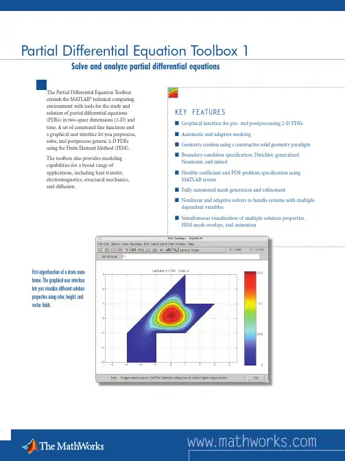
The Partial Differential Equation T oolbox extends the MATLAB® technical computing environment with tools for the study and solution of partial differential equations (PDEs) in two-space dimensions (2-D) and time. A set of command-line functions and a graphical user interface let you preprocess, solve, and postprocess generic 2-D PDEs using the Finite Element Method (FEM).Partial Differential Equation Toolbox 1 Solve and analyze partial differential equationsWorking With the Partial Differential Equation ToolboxThe Partial Differential Equation T oolbox lets you work in six modes from the graphi-cal user interface or the command line. Each mode corresponds to a step in the process of solving PDEs using the Finite Element Method.• D raw mode lets you create Ω, the geometry, using the constructive solid geometry (CSG) model paradigm. The graphical interface provides a set of solid building blocks (square, rectangle, circle, ellipse, and polygon) that can be combined to define complex geometries.•B oundary mode lets you specify conditions on different boundaries or remove sub d omain borders.• P DE mode lets you select the type of PDE problem and the coefficientsc, a, f, and d . By specifying the coefficients for each subdomain independently, you can represent different material properties.• M esh mode lets you control the fully automated mesh generation and refinement process.• S olve mode lets you invoke and control the nonlinear and adaptive solver for elliptic problems. For parabolic and hyperbolic PDEproblems, you can specify the initial values and obtain solutions at specific times. For the eigenvalue solver, you can define the interval over which to search for eigenvalues.• P lot mode lets you select from different plot types, including surface, mesh, and contour. Y ou can simultaneously visualize multiple solution properties using color, height, and vector fields. The FEM mesh can be overlaid on all plots and shown in the displaced position. For parabolic and hyperbolic equations, you can animatethe solution as it changes with time.Defining and Solving Partial Differential EquationsWith the Partial Differential Equation T oolbox, you can define and numerically solve different types of PDEs, including elliptic, parabolic, hyperbolic, eigenvalue, nonlinear elliptic, and systems of PDEs with multiple variables.Elliptic PDEThe basic scalar equation of the toolbox is the elliptic PDEwhere is the vector (∂/∂x ,∂/∂y ), and c is a 2-by-2 matrix function on Ω, the bounded planar domain of interest. c, a, and f can be complex valued functions of x and y.Nonlinear Elliptic PDEA nonlinear Newton solver is available for the nonlinear elliptic PDEwhere the coefficients defining c, a, and fcan be functions of x, y, and the unknown solution u. All solvers can handle the PDE system with multiple dependent variablesY ou can handle systems of dimensiontwo from the graphical user interface.An arbitrary number of dimensions canbe handled from the command line.The toolbox also provides an adaptivemesh refinement algorithm for ellipticand nonlinear elliptic PDE problems.Using the graphical user interfaceto define the complex geometryof a wrench, generate a mesh,and analyze it for a given loadconfiguration.Toolbox Application ModesThe Partial Differential Equation T oolbox graphical interface includes a set ofappli c ation modes for common engineeringand science problems. When you select a mode, PDE coefficients are replaced with appli c ation-specific parameters, such asY oung’s modulus for problems in structural mechanics. Available modes include:• Structural Mechanics - Plane Stress• Structural Mechanics - Plane Strain• Electrostatics• Magnetostatics• AC Power Electromagnetics• Conductive Media DC• Heat Transfer• DiffusionThe boundary conditions are alteredto reflect the physical meaning of the different boundary condition coefficients. The plotting tools lets you visualizethe relevant physical variables for the selected application.Required ProductsMATLABRelated ProductsOptimization Toolbox. Solve standardand large-scale optimization problems.Statistics Toolbox. Apply statistical algorithms and probability models.Symbolic Math Toolbox andExtended Symbolic Math Toolbox. Perform computations using symbolic mathematics and variable-precision arithmetic.Platform and System RequirementsFor platform and system requirements, visit /products/pde ■8557v02 10/03For demos, application examples,tutorials, user stories, and pricing:•Visit •Contact The MathWorks directlyUS & Canada 508-647-7000Benelux +31 (0)182 53 76 44France +33 (0)1 41 14 67 14Germany +49 (0)241 470 750Italy +39 (011) 2274 700Spain +34 93 362 13 00Switzerland +41 (0)31 954 20 20UK +44 (0)1223 423 200Visit to obtaincontact information for authorizedMathWorks representatives in countriesthroughout Asia Pacific, Latin America,the Middle East, Africa, and the restof Europe.Visualization tools provide multiple ways to plot results. A contourplot with gradient arrows shows the temperature and heat flux.The temperature gradient is displayed using 3-D plotting tools.T el: 508.647.7000 info@ © 2003 by The MathWorks, Inc. MATLAB, Simulink, Stateflow, Handle Graphics, and Real-Time Workshop are registered trademarks, and TargetBox is a trademark of The MathWorks, Inc. Other product or brand names are trademarks or registered trademarks of their respective holders.。

（8）
因此,对有一对磁极的三相异步电动机来说,旋转磁 场的角速度与交流电角频率大小相等。对有 对磁极的三 相异步电动机,由于电度角等价于 倍机械角,所以旋转磁 场可表示为：
（9）
78
电子技术教育 Electronics Education
对磁极的三相异步电动机的磁场波在气隙中传播的 线速度和角速度分别为：
在MATLAB主窗口中，选择File菜单中的New菜单项， 打开界面设计模版，选择相应的控件设计界面，界面中
包含：
（1）两个坐标图，一个是z方向代表磁感应强度B的 三维视图，一个是前一图沿x、y坐标为（0，1）即 处 切开的二维视图，y轴代表B，x轴代表 ；
（2）两个命令按钮，分别绘制磁场分布图形和结束
（2）
图1
图2 （参见右栏）
若AX绕组不是通以直流 ，而是通以正弦交流
，则上面的分析可知，此时磁感应强度基波
分量的表达式为：
（3）
由式（3）表示的磁场称为脉动磁场，式中 是正弦
图1
图2
电流在气隙中产生的脉动磁场基波分量的幅值。显然，
若电机中通以对称的三相交流电，则BY、CZ绕组中产生 的磁感应强度基波分量可表示为：
79
周 鹏 张克金 陈万平 王 静 (曲阜师范大学物理工程学院)
摘 要：以电机旋转磁场的演示系统制作为例，本文研究了MATLAB的GUI功能在开发交互式教学演示软件 中的应用。
关键词：电机；旋转磁场；MATLAB；GUI
Designing Demo Software of Motor's Rotating Magnetic Field Based on MATLAB
参考文献： [1] 贾启民．电磁场[M]．北京：高等教育出版社，2001． [2] 郭木森，黄元梅．电工学（第三版）[M]．

MATLAB的主要功能1. 数值计算和符号计算功能2. 绘图功能3. MA TLAB语言体系4. MA TLAB工具箱Matlab语言的特点编程简单，类似于其他语言，如C集成度更高，扩展性更好数学问题数值解能力强大由Maple内核构成的符号运算工具箱可以继承Maple所有解析解的求解能力在数学、工程领域各种“工具箱”强大的系统仿真能力，Simulink建模Mathlab的命令窗口（command window)1. 命令窗口的作用命令窗口处于窗口的右侧，用来输入数据、操作命令和显示运行结果。

命令窗口(Command Window)是用户使用的主要场所，此时，可以输入变量、数组及运算命令，进行一些简单的运算；用↑↓←→键搜索、修改以前使用过的命令操作, 用clc清除窗口; 用help sqrt ( help input …)寻求有关帮助;2. 命令行的输入规则一个命令行输入一条命令，命令行以回车结束。

一个命令行也可以输入若干条命令，各命令之间以逗号分隔，若前一命令后带有分号，则逗号可以省略。

如果一个命令行很长，要加续行符（三个小黑点…）。

3. 命令行的编辑各种编辑键，如方向键，删除键等，基本同其它软件，可见课本. 比较特殊的是：上箭头键(up)可调入前一行命令.4. 常用操作系统命令●>disp(x) 显示x的内容，与x 的区别是：前者仅显示x的内容，后者多个"x=".●> diary 建立一个diary文件，如diary abc.dia. 文件名和扩展名可任取，并开始记录此后MA TLAB的所有操作，用diary off停止记录，并可用type abc.dia显示记录内容.●> path 显示当前搜索路径●管理文件的命令：●> what, 显示当前目录下的m, mat, mex文件●> dir, 或> ls, 显示当前目录下的所有文件●> cd path 改变当前目录为path●> cd, >chdir, >pwd, 都可显示当前的工作目录●> type abc, 显示文件abc.m的内容●> delete abc.m, 删除m文件abc.m(必须有扩展名)●> which abc, 显示abc.m所在的目录，若要显示其它类型文件的目录，必须加扩展名.●> quit, 退出MATLAB.MATLAB的通用命令管理命令和函数：功能强大的工具箱是MATLAB的另一特色。

MatlabPDE工具包在电场电势可视化教学中的应用作者：张勇吴卫华来源：《江苏理工学院学报》2020年第02期摘要：为了使学生更易理解电场、电势以及两者之间的关系，需要在电场电势教学中采用可视化教学方式。

展示了如何利用Matlab PDE工具包描述电场、电势以及两者之间的关系，并进一步提出了应用实例。

PDE工具包可以形象地表示出帶电体的电场、电势以及两者之间的关系，并且在使用过程中不需要任何编程基础。

Matlab PDE工具包可以在大学物理电场电势教学中广泛地加以推广。

关键词：Matlab;PDE工具包;可视化教学;电场;电势中图分类号：O441;G642.4 文献标识码：A 文章编号：2095-7394（2020）02-0087-07“大学物理”是大学理工科非物理类专业学生一门重要的通识必修基础课。

由于课程中的某些概念比较抽象，学生不易理解，因此，需要结合图形将难以理解的物理概念及公式形象地表示出来，即构建可视化的大学物理教学方式。

在电场电势章节教学中，我们发现，学生对复杂带电体的电场、电势以及两者之间关系的理解有困难，虽然大多数教材都配套了对应的PPT（Microsoft Office PowerPoint），其中也含有一些对于带电体电场以及电势的形象描述，但是仍不够全面，这就要求教师尝试掌握一种直观、形象描述电场、电势的方法，采用可视化教学方式十分必要。

Matlab是由美国MathWorks公司出品的一款商业数学软件，可实现矩阵运算、绘制函数和数据、实现算法等应用。

目前，Matlab在科研及教学领域已得到普及，并且被广泛应用于大学物理可视化教学。

[1-4]但是，在应用过程中需要使用者有相应的Matlab编程基础，这对初学者而言还是有一定困难的。

Matlab中的PDE工具包（Partial Differential Equation （PDE） Toolbox）是一款强大的软件工具包，它为使用者求解偏微分方程提供了方便。

matlab完整版（三相闭环）三闭环错位选触⽆环流可逆直流调速系统1. 系统仿真应⽤软件及其简介三闭环错位选触⽆环流可逆直流调速系统仿真应⽤的软件是MATLAB 7.0。

MATLAB是为了在科学研究和⼯程应⽤中，克服⼀般语⾔对⼤量数学运算，尤其是涉及矩阵运算时编制程序复杂、调试⿇烦等困难，美国Math Works公司于1967年构思并开发了矩阵实验室（Matri Laboratory’，MATLAB）软件包。

经过不断的更新和扩充，该公司于1984年推出了MATLAB的正式版，特别是1992年推出具有跨时代意义的MATLAB 4.0版，并于1993年推出其微机版，以配合当时⽇益流⾏的Microsoft Windows 操作系统⼀起使⽤。

截⽌到2005年，该公司先后推出了MATLAB 4.x，MATLAB 5.x，MATLAB 6.x，MATLAB 7.xD等版本，该软件的应⽤范围越来越⼴。

常见的MATLAB⼯具箱有以下⼏种。

Control System Toolbox——控制系统⼯具箱Communication Toolbox——通讯⼯具箱Financial Toolbox——财政⾦融⼯具箱System Identification Toolbox——系统辨识⼯具箱Fuzzy Logic Toolbox——模糊逻辑⼯具箱Higher-Order Spectral Analysis Toolbox——⾼阶谱分析⼯具箱Image Processing Toolbox——图象处理⼯具箱computer vision system toolbox----计算机视觉⼯具箱LMI Control Toolbox——线性矩阵不等式⼯具箱Model predictive Control Toolbox——模型预测控制⼯具箱µ-Analysis and Synthesis Toolbox——µ分析⼯具箱Neural Network Toolbox——神经⽹络⼯具箱Optimization Toolbox——优化⼯具箱Partial Differential Toolbox——偏微分⽅程⼯具箱Robust Control Toolbox——鲁棒控制⼯具箱Signal Processing Toolbox——信号处理⼯具箱Spline Toolbox——样条⼯具箱Statistics Toolbox——统计⼯具箱Symbolic Math Toolbox——符号数学⼯具箱Simulink Toolbox——动态仿真⼯具箱Wavele Toolbox——⼩波⼯具箱DSP system toolbox-----DSP处理⼯具箱这⾥只重点介绍MATLAB在本系统中Simulink的仿真环境。

●提供廣泛的訓練及學習函式●提供Simulink的類神經網路block●可自動將MATLAB產生的類神經網路物件轉成Simulink 模型●提供前處理及後處理函式改善類神經網路訓練及效能●提供視覺化函式更容易瞭解類神經網路之效能(Preceptron)、倒傳遞網路(Backpropagation)、自組織映射網路(SOM)、徑向基網路(Radial Basis Network)、學習向量量化網路(LVQN)..等.◎ Curve Fitting Toolbox(曲線契合工具箱)產品特色●可透過圖形化使用者介面或指令列操作各種功能●可作資料前置處理的例行程序設定，例如資料排序、分割、平滑化、及除去界外值(outlier)等●擁有線性或非線性參數契合模型的龐大的函式庫，與最佳化的起始點(starting points)以及非線性模型參數的解題器●多樣的線性和非線性契合方法，包括最小平方法、加權最小平方法、或強韌契合程序(robustfitting procedures) (上述全部支援限制係數範圍或不限制係數範圍的功能)●客製化的線性或非線性模型發展●使用Splines或內插法(interpolants)進行非參數(Nonparametric)契合●支援內插法、外插法、微分以及積分計算簡介1.功能就是可將客戶的資料畫成圖形，接著提供現有標準的一些數學式子來找出符合這圖形的方程式，例如y=ax+bx^2+cx^3。

2.裡面有提供許多的數學式子，也可讓User自定自己的數學函式，而此工具箱可幫客戶算出數學式子的係數(如a,b,c等)3.提供polynomial, exponential, Fourier, rational等數學model給客戶Note: 此套工具不能作曲面的契合，即是如果客戶要求要作y=ax1+bx2 找出a與b，是不可以的，因為此工具箱只能找出單一變數x的係數。

建議他們購買OP and SP 解決他們的問題。

基于 matlab 的对流弥散衰减方程求解与应用一、引言对流弥散衰减方程（Convection-Dispersion-Attenuation Equation，CDAE）是描述污染物在地下水中运移和转化的基本数学模型，其求解对于地下水污染的研究和防治具有重要意义。

本文将介绍基于 matlab 的对流弥散衰减方程求解与应用。

二、对流弥散衰减方程对流弥散衰减方程是由美国环境保护署（Environmental Protection Agency，EPA）在20世纪70年代提出的，其数学形式为：$$\frac{\partial C}{\partial t} = D \frac{\partial^2 C}{\partial x^2} - v \frac{\partial C}{\partial x} - kC$$其中，$C$ 为污染物浓度；$t$ 为时间；$x$ 为空间坐标；$D$ 为分子扩散系数；$v$ 为平均线速度；$k$ 为吸附系数。

该方程描述了污染物在地下水中的扩散、对流和吸附过程。

三、matlab 求解1. 前置条件在使用 matlab 求解 CDAE 前，需要先安装 Partial Differential Equation Toolbox 和 Optimization Toolbox。

2. 初值问题求解初值问题是指在已知初始条件下，求解方程在一段时间内的解。

对于CDAE，可以使用 matlab 的 pdepe 函数进行求解。

pdepe 函数的输入参数包括：- pdex1: 定义空间区域；- pdex2: 定义时间区域；- pdex3: 定义方程的系数；- pdex4: 定义初始条件；- pdex5: 定义边界条件。

以下是一个求解 CDAE 初值问题的示例代码：```matlabfunction [c, f, s] = cdae(x, t, u, dudx)D = 1; v = 0.1; k = 0.01;c = 1;f = D*dudx - v*u;s = -k*u;endfunction u0 = initialCondition(x)u0 = exp(-x.^2);endfunction [pl, ql, pr, qr] = boundaryConditions(xl, ul, xr, ur, t)pl = ul; ql = 0;pr = ur; qr = 1;endxmesh = linspace(0, 20);tspan = linspace(0, 10);sol =pdepe(0,@cdae,@initialCondition,@boundaryConditions,xmesh, tspan);surf(xmesh,tspan,sol(:,:,1))xlabel('Distance x')ylabel('Time t')zlabel('Concentration C')```3. 边值问题求解边值问题是指在已知边界条件下，求解方程在整个空间区域内的解。

MATLAB R2009a\help\product help\Partial Differential Equation Toolbox\Graphical User Interface this chapter discusses the graphical user interface (GUI) pdetool. The main components of theGUI are the menus, the dialog boxes, and the toolbar.PDE Toolbox 求解椭圆、抛物、双曲方程的基本步骤第一步：在MATLAB命令窗口，输入命令>> pedtool进入PDE Toolbox窗口第二步：建立几何模型在toolbar中选择几何图形，如建立单位圆，则点击第3或第4个按钮，用鼠标的右键，click-and-drag，创立一个圆c1双点击圆c1，弹出dialog box，输入几何参数第三步：输入边界条件点击输入边界条件。

若所有边界条件都是齐次的第一类边界条件，此步可省略。

第四步：输入偏微分方程参数点击输入偏微分方程参数。

第五步：划分网格点击一次，初步划分网格。

点击多次，细划网格。

单元圆细化两次的结果第六步：输入初始条件若方程是椭圆的，此步可省略。

点击菜单中的 Parameters 选项。

若方程是抛物的，则需输入初始位移条件及计算参数若方程是双曲的，则需输入初始位移条件、初始速度条件及计算参数第七步：求解有限元方程点击求解有限元方程。

第八步：绘图点击绘图。

利用绘图选项，将计算结果进行可视化输出。

下面是两个编程算例。

泊松方程边值问题单位圆域内泊松方程齐次边值问题其精确解为试求泊松方程问题的数值解并与精确解比较。

解 (1) 建立有限元模型在MATLAB 命令窗口，输入命令>> pedtool进入PDE Toolbox 窗口在toolbar 中点击第3或第4个按钮，用鼠标的右键，click-and-drag ，创立一个圆c1()⎪⎩⎪⎨⎧=+=<+=+-1,01,12222y x u y x u u yy xx ()22141y x u --=双点击圆c1，输入几何参数输入边界条件（略）。

二阶偏微分方程的 Matlab有限元法求解摘要：本文基于偏微分方程有限元法求解原理，运用Matlab中的偏微分方程工具箱（PDE Toolbox）对三类典型的二阶偏微分方程：椭圆型方程、双曲线型方程和抛物线型方程算例进行求解，为求解偏微分方程的提供参考。

关键词：偏微分方程，有限元，Matlab偏微分方程工具箱0引言偏微分方程定解问题是描述许多自然现象或工程问题的最重要的数学模型，应用非常广泛[1]。

解析法只能求解非常简单的偏微分方程，远远不能满足科学研究和工程实际的需要。

随着计算机技术和科学计算的迅速发展，数值解法成为求解偏微分方程的重要工具[2-3]。

数值解法将连续问题离散化，最后将偏微分方程化成线性代数方程组。

根据离散化方法不同，偏微分方程数值解法主要有差分法和有限元法。

有限元法是分片定义试函数与变分原理相结合的产物。

它能适应各种形状的区域，且通用性强，现已成为求解偏微分方程定解问题的一种有效数值方法[4]。

本文首先简述了偏微分方程有限元法原理，然后，对Matlab中的偏微分方程工具箱（Partial Differential Equations Toolbox）的功能和求解思路进行了阐述[5-6]，最后，给出了用PDE Toolbox求解椭圆方程、、双曲线方程和抛物线方程的计算实例。

1偏微分方程有限元法原理偏微分方程有限元法的基本思想是将实际上连续的整个求解域进行离散化处理，即用一些假想的面或线将求解域分割为一系列的单元，各个单元之间仅在有限个节点处相互连接。

取未知函数的节点值作为基本未知量，在每个单元上选取一个近似的插值函数表示单元中场函数的分布规律。

利用变分原理来获得单元的刚度方程，然后按一定的规则把所有单元的刚度方程组集合起来，经适当的边界条件处理，便得到整个系统的总体方程组。

这样，偏微分方程便转化为一组常微分方程。

最后，求解总体方程组，得到节点值和用插值函数确定整个求解域上的场函数。

非支配排序遗传算法的动压轴承形状多目标优化庞晓平;陈进【摘要】In order to overcome the shortcoming caused by taking the eccentricity as the initial design variables in the shape optimization model, i. e. , the optimized shape was localized in the original shape , a new mathematic model of multi-objective shape optimization for hydrodynamic journal bearings was built through the general film thickness equation based on the Fourier series. In the model, the objective function is minimization of oil leakage and power loss, which is subjectedto the minimum oil film thickness and the minimum bearing capacity, and the coefficients of general oil film thickness are design variables. Themulti-objective optimization for the profile design of a hydrodynamic journal bearing is accomplished using a modified non-dominated sorting genetic algorithm II (NSGA- Ⅱ ) . The governing equations based on the general film thickness were solved by Matlab PDE (partial differential equation) toolbox. The results of a case study show that the bearing shape obtained by multi-objective optimization based on the general film thickness equation is not limited by the original shape. In addition,a Pareto-optimal set is obtained, where, for one of the optimized non-circle bearings with the maximum load capacity, the power loss and leakage rate are decreased by 80.8% and three orders of magnitude, respectively, compared with that just taking the load capacity as the objective function.%为了克服以偏心率为初始参数的轴承优化模型优化结果局限于原始形状的缺点,提出用傅里叶级数表示通用膜厚方程,建立了多目标形状优化设计数学模型.应用基于非支配排序遗传算法,以最小功耗和最小侧漏流速为目标、最小油膜厚度和最小承载力为限制条件,以通用膜厚方程系数为设计变量,进行了轴承形状的多目标优化设计,并用Matlab偏微分方程工具箱求解基于通用膜厚的控制方程.实例分析结果表明:基于通用膜厚方程的多目标优化后的轴承形状不受固有型线的限制；在保证最大承载力的基础上,优化后的非圆轴承与仅以最大承载力为单目标优化的结果相比,最小功耗下降了80.8％,最小侧漏流速比优化前下降了3个数量级,并得出了Pareto最优解集.【期刊名称】《西南交通大学学报》【年(卷),期】2012(047)004【总页数】7页(P639-645)【关键词】动压径向轴承;形状优化;NSGA-Ⅱ;多目标优化;Pareto最优解集【作者】庞晓平;陈进【作者单位】重庆大学机械传动国家重点实验室,重庆400030;重庆大学机械传动国家重点实验室,重庆400030【正文语种】中文【中图分类】TH133.37为降低转动支承件的设计成本与运行成本，提出轴承最优化设计概念.轴承优化设计的目标函数有:增加承载力、降低摩擦损耗、加强稳定性、降低润滑剂的供应量、削弱温升等.动压轴承形状的设计本质上是一个多目标优化问题[1].目前，许多学者对动压轴承系统进行了多目标优化设计[1-6]，以轴承半径间隙、宽径比、油槽位置、供油量和润滑油粘度，供油压力等为设计变量，以最小温升、最小油膜厚度、最小油膜比压等为限制条件，以最小化功率损耗、最小化侧漏流速、最小化温升等为目标函数进行了多目标优化.设计变量中只有半径间隙与轴承形状直接相关，通过调整偏心率改变轴承的性能，优化后的形状仍与初始形状相同(例如圆轴承).任意形状轴承的设计和制造生产已经成为可能，文献[7-11]分别以最大承载力或最高稳定性为目标进行了任意形状轴承的单目标优化研究，阐述了研究非圆形状轴承对轴承设计的重要意义.针对动压径向轴承形状设计及优化存在的问题，本文提出基于傅里叶级数的通用轴承型线表征形式，以最小化侧漏流速和最小化功率损耗为目标函数，以通用轴承型线方程的系数为设计变量，以最小油膜厚度和最小承载力为限制条件，建立轴承形状多目标优化模型，采用全局寻优方法——改进的非支配排序多目标遗传算法(NSGA-Ⅱ)，用Matlab求解偏微分方程工具箱编程，寻求轴承形状多目标优化的Pareto最优前沿集.1 优化模型1.1 几何理论轴承形成动压的几何要素:轴与轴承内表面之间具有楔形间隙，使润滑流体由间隙大端向间隙小端运动.假设整个间隙充满油液，楔形间隙可以用油膜厚度来表征.因此，可通过油膜厚度表达式研究楔形间隙的几何关系.圆柱轴承的几何关系如图1所示.图1中，O为轴心;Oj为轴承中心;r为轴半径;R 为轴承半径;ω为轴转动角速度;h为油膜厚度;θ为轴转动的角度;e为偏心率.用三角形正弦定理可以得出油膜厚度:式中:c和e分别是动压轴承半径间隙和偏心率，是轴承的位置参数.式(1)即为传统优化方法常用的圆柱轴承膜厚方程，通过调整c和e实现油膜厚度的改变，其轴承的形状仍然为圆.图1 圆柱轴承几何关系Fig.1 Geometric relation of cylindrical bearing以圆轴承膜厚方程为基础建立的优化模型不能对轴承形状进行优化，它只是调整了轴承与轴的相对位置，通过调整偏心率改变轴承的动压性能.为获得全局最优的轴承形状，建立统一的形状优化模型，轴承通用膜厚表达式成为必要.假定动压轴承内表面周向为任意形状，轴向不变，轴颈为圆柱，轴颈顺时针旋转，轴承不动，其几何形状如图2所示.图2中，ρ(θ)为轴承极径;h(θ)为油膜厚度.图2 动压轴承楔形间隙几何示意Fig.2 Geometric schematic of wedge-shape gap of hydrodynamic bearing文献[12]提出基于傅里叶级数的通用无量纲油膜厚度方程:式中:a0、an和bn为待定系数，是形状优化的设计变量;n为傅里叶级数的阶数. 该通用膜厚表达式不仅适用于现有常用的经典轴承形状，还易于扩展出新的楔形几何形状.通过调整待定系数和傅里叶级数的阶数，可以得到椭圆、三油叶、多油叶等不同形状的轴承[12].1.2 控制方程本文根据动压润滑原理建立无量纲雷诺方程.用Matlab中的PDE(partial differential equation)工具箱求解比压，用数值积分求解功率损耗和侧漏流速.设润滑介质为不可压缩的牛顿液体，稳态层流且无滑移，忽略不计彻体力和惯性力，沿膜厚方向恒温恒压，满足假设条件常用的无量纲雷诺方程[7]为:式中:l轴承宽度;d为轴径;p为轴承无量纲比压;μ为润滑液的粘度.式(3)为二阶非线性偏微分方程，没有解析解，用Matlab的PDE工具箱中有限元数值方法，基于雷诺边界条件求解比压.用PDE工具箱解偏微分方程简化了有限元中划分网格的过程，可用简单命令mesh和remesh把求解区直接划分成8 288个Delaunay类型网格.完成比压计算后，其它性能指标就可利用比压值计算得到.承载力F可以通过对比压的积分得到，这里采用Gümbel边界条件，即积分时只积分正值，量纲承载力为:侧漏流速和摩擦阻力的无量纲形式如下:相应的量纲形式为:功率损耗则为:轴承多目标优化模型的目标函数为最小化功耗W和侧漏流速Q，限制条件为最小油膜厚度hmin和最小承载力Fmin.限制条件的处理采用惩罚目标函数f(X)，设计变量 X={a0，a1，b1，…，aibi，…，an，bn}，i=1，2，…，n，n可以通过目标函数对无穷项级数的逐步逼近确定.2 优化方法——NSGA-Ⅱ在多目标优化中，目标之间相互冲突，很难找到所有目标均为最优的最优解，而是存在一系列有效解，其特点是至少存在一个目标优于其他解的解，该解称为非支配解，或Pareto解，这些解的集合即为Pareto最优解集.求解多目标优化问题的主要任务是求该优化问题的Pareto最优解集[13-14].在多目标优化算法中，多目标遗传算法(non-dominant sort in genetic algorithm，NSGA[15])的应用研究最为广泛.NSGA算法将非支配排序思想引入遗传算法，把多个目标函数的计算转化为虚拟适应度的计算，用于求解多目标优化问题.NSGA的基本原理是基于对个体的几层分级实现种群的非支配排序，选择操作执行个体被排成一类，这些个体共享虚拟适应度值，逐步对剩余个体进行分级并赋予相应的虚拟适应度.NSGA-Ⅱ是以NSGA为基础的改进非支配排序遗传算法[15]，用快速非支配排序过程、精英保留策略及无参数小生境操作算子，克服传统NSGA的计算复杂度高、非精英保存策略及无需特别指定共享半径的缺点，其算法过程如图3所示.图3中:Pt为第t代种群，种群规模为 N;Qt为由Pt产生的子种群.为保护进化过程中出现的优秀个体，采用精英保留策略，将Pt和Qt合并形成个体数为2N的混合种群Rt，并对Rt进行非支配排序，得 F1，F2，…，Fk共 k级个体群，依次选择前面的个体群.当选择到第Fi级个体群时，总选择个体数超过种群个体数N，则基于小生境技术对Fi进行拥挤度排序，依次选择较好的个体，直至选择个体数达到N，从而形成第t+1代种群Pt+1.轴承形状多目标优化求解流程如图4所示.图3 NSGA-Ⅱ步骤Fig.3 Procedures of NSGA-Ⅱ图4 NSGA-Ⅱ算法流程图Fig.4 Flow chart of NSGA-ⅡNSGA-Ⅱ的两个关键技术是非支配排序和确定拥挤距离[15].根据等级和拥挤距离，用赛事选择方法从群体里选择父代.设计者根据需要在优化后的最优解集里选择，不需要像常用的多目标优化算法通过选择权重因子把多目标变成单目标，降低了对设计经验的要求.用遗传算法求解优化模型，确定优化算法的求解过程，编制优化程序，集成有限元计算程序.本文选用的群体规模为20，遗传代数为100代，交叉概率为 0.90，变异概率为 0.01.3 算例分析根据本文提出的算法及数学模型，用Matlab编程对轴承进行形状优化设计.表1列出了文献[7]形状优化的参数及结果.以最大承载力为目标，离散的廓线点数据为设计变量优化出了比全圆轴承性能更优的任意形状轴承.本文算法计算的承载力(表1括号中数值)与有限差分方法的结果基本符合，说明用Matlab的PDE工具箱求解Reynold方程的适用性.由于未考虑进油压力与油槽的影响，功耗、侧漏流速的计算结果有一定误差，但并不影响本文对动压轴承形状的研究.为了方便比较，选用相同的设计参数，用多目标优化相应的圆柱轴承和任意廓线的轴承.以最小功率损耗和侧漏流速为目标，文献[7]优化得出的最大承载力为限制条件，即要求承载力大于优化后的最大值，用通用型线方程的系数作为设计变量.表2是通用型线方程中n=1(即要求优化结果为圆轴承)时优化后的部分数据，优化结果和表1对圆轴承优化的结果相似.因为当n=1时，轴承的廓线为圆，只能调整偏心率和半径间隙，由于通用型线的形状优化方法和传统方法实质是相同的，在保证最大承载力时形状就已经确定，再以功耗、侧漏流速为目标进行优化的结果没有改变.表3是通用型线方程中n=3(即优化结果不受圆轴承的限制)时优化后的部分数据，可能得到任意的轴承形状.文献[8]已经证明，在以最大承载力为目标时，用基于通用型线的形状优化方法其结果优于当前其它优化方法得到的结果.以文献[7]中优化的最大承载力2 003 N为多目标优化限制条件，要求最大承载力大于2 003 N.从表3可以看到，多目标优化后的功耗、侧漏流速远小于表1中优化出的任意形状轴承的数据，且最大比压小于表1中的优化结果.例如，比较表3中第2组数据与表1中的非圆轴承在多目标优化前的性能数据，在保证最大承载力的基础上，多目标优化后的非圆轴承最小功耗由101 W降至19.4 W，下降了80.8%;最小侧漏流速由0.216×103cm3/s降至0.117 cm3/s，下降了3个数量级，这充分证明了对径向动压轴承进行多目标形状优化的必要性.图5(a)和图5(b)分别是通用型线方程当n=1和3时的Pareto最优前沿可视图.图6(a)和图6(b)分别是当n=1和3时优化后的1组轴承形状示意图(分别对应表2和表3中的前3组参数).图6(a)中型线只改变了轴承的大小，其形状还是圆，但图6(b)中型线相对于圆改变较大.前面分析表3数据时已经提出优化后的任意型线的轴承性能优于圆轴承，这再次说明了对非圆轴承形状研究的重要性和必要性.比较图6(b)中的3组轴承型线，表3显示轴承2的侧漏流速相对于轴承1和3的小，但功耗大，此结果符合轴承润滑理论，因为轴承2的间隙小于轴承1和3的间隙，间隙中的润滑液较少，则侧漏流速也较小;但间隙小，温升则较大，产生的摩擦力较大，摩擦损耗高.表1 Boedo完成的单目标形状优化参数与结果Tab.1 Parameters and resultsof single objective optimization by Boedo注:括号中数值为本文算法的计算结果.d/mm l ω最优形状30 30 5 2 000×2π/mm粘度/(mPa·s－1)/(rad·s－1)优化目标hmin/μm Fmax/N W/W Q/(cm3·s－1) Pmax/MPa 5 1 882.1 15.30 0.169 4.55 60任意形状圆形5 (1 882.4)(16.94) (0.179) (5.02) 圆形5 2 003.0 101.10 0.216 ×103 5.52表2 通用膜厚方程中n=1时的多目标形状优化结果Tab.2 Multi-objective shape optimization results at n=1 in the general film thickness equation优化变量a0 a1 b/W Pmax/MPa Fmax/N hmin/μm阶拥挤距离－0.8370.000 1.838 0.176 17.0 5.09 1.88 5.01 1 1优化目标Q/(cm3·s－1) W选择参数∞－0.632 0.000 1.639 0.132 18.7 4.75 1.89 5.03 1 ∞－0.821 0.000 1.822 0.172 17.1 5.07 1.88 5.01 1 0.281－0.646 0.000 1.655 0.135 18.5 4.75 1.88 5.05 1 0.259－0.774 0.000 1.780 0.162 17.4 4.98 1.885.03 1 0.252表3 通用膜厚方程中n=3时的多目标形状优化结果Tab.3 Multi-objective shape optimization results at n=3 in the general film thickness equation设计变量a0 a1 b1 a2 b2 a3 b优化目标Q/(cm3·s－1)W/Pmax Fmax hmin距离－0.766 －0.450 －0.128 0.213 0.111 0.008 1.825 0.180 17.5 4.64 2.00 5.21 1 3 W /MPa /kN /μm选择参数阶拥挤∞－0.520 －0.262 －0.016 －0.076 －0.042 0.138 1.577 0.117 19.4 4.91 2.04 5.00 1 ∞－0.719 －0.454 －0.117 0.176 0.127 0.034 1.782 0.170 17.8 4.85 2.01 5.29 1 0.38－0.522 －0.263 －0.014 －0.065 －0.042 0.131 1.583 0.117 19.3 4.79 2.01 5.03 1 0.35－0.650 －0.352 －0.077 0.046 0.007 0.088 1.736 0.150 18.0 4.30 2.015.08 1 0.34基于NSGA-Ⅱ的多目标轴承形状优化模型仍然是以傅里叶级数为基础建立通用膜厚的优化模型.前面的分析没考虑傅里叶级数无穷项级数n的取值问题，直接赋值1和3进行讨论.在单目标优化中采用逐次逼近方法来确定无穷级数，在多目标优化中仍然可采用该方法，只是不能确定一个确切的容差值，但是，NSGA-Ⅱ的优化方法可以画出Pareto最优前沿可视图，从可视图中可以直观地判定无穷级数的取值.图7为不同级数n对应的基于NSGA-Ⅱ优化方法的动压径向轴承多目标形状优化Pareto最优前沿可视图，限制条件最小承载力采用了Boedo优化型线为圆的最大承载力(1 882.1 N).从图6看出，n=2的优化结果比n=1的优化结果有明显改善.随着n增加，其Pareto最优前沿集停留在n=2解集附近，从图7中看不出有明显改善，所以，本例中可以说当n≥2时无穷级数多目标优化取得最优值，更高阶的轴承型线对应的功耗和侧漏流速曲线收敛于n=2时的曲线附近.图5 当n=1和n=3时的Pareto最优前沿可视图Fig.5 Pareto optimal frontat n=1 and n=3图6 当n=1和n=3时轴承的最优型线示意图Fig.6 Schematic diagram of optimal profiles at n=1 and n=3图7 限制条件Fmin=1 882.1 N下的Pareto最优前沿集可视图Fig.7 Pareto optimal front under the constraint Fmin=1 882.1 N4 结论分析了目前轴承形状优化研究的局限性，用NSGA-Ⅱ对动压径向轴承进行了形状多目标优化，得出以下结论:(1)以圆轴承膜厚方程为基础建立优化模型不能实现对轴承形状的优化，只是调整了轴承与轴的相对位置，通过调整偏心率改变轴承性能.(2)基于傅里叶级数建立不受经典形状限制的通用膜厚表达式，便于建立统一的优化数学模型，通过寻优手段得到最终的任意形状最优径向动压轴承.(3)用NSGA-Ⅱ优化方法，利用惩罚因子处理非线性约束条件，成功地进行了动压轴承形状多目标优化，得出Pareto前沿解集，有效避免了一般多目标优化中权重因子的确定.(4)在多目标优化中，对通用膜厚方程无穷级数仍然可采用逐步逼近的方法寻找收敛点.(5)利用现有工具Matlab偏微分PDE工具箱求解基于动压润滑原理建立的优化模型，简化了复杂的编程过程.(6)对于建立动压径向轴承通用型线完整理论，构造具有最佳性能的动压轴承型线，具有重大的理论意义和应用价值;同时，对以楔形效应为工作原理的机械及通过微小间隙润滑进行传动的传动装置廓线理论研究的深入发展也具有重要推动作用.参考文献:【相关文献】[1]DOBRICA M B， FILLON M，PASCOVICI M D.Optimizing surface texture for hydrodynamic lubricated contacts using a mass-conserving numerical approach[J]. Proceedings of the Institution of Mechanical Engineers，Part J:Journal of Engineering Tribology，2010，224(8):737-750.[2]HIRANI H.Multiobjective optimization of a journal bearing using the Pareto optimality concept[J].Proc.Instn Mech.Engrs，Part J:J.Engineering Tribology，2004，218(2):323-336.[3]HIRANI H ，SUH N P.Journal bearing design using multiobjective genetic algorithmand axiomatic design approaches[J].Tribology Int.，2005，38(1):481-491.[4]HIRANIH. Multiopjective optimization ofjournal bearing using mass conserving and genetic algorithms[J]. J. Engineering Tribology， 2005，219(1):235-249.[5]ZENGEYA M，GADALA M.Optimization of journal bearings using a hybridscheme[J].J.Engineering Tribology，2007，21(3):591-609.[6]HIRANI H，RAO T V V L N，ATHRE K，et al.Rapid performance evaluation of journal bearing[J].Tribology Int.，1997，11(6):825-834.[7]BOEDO S，ESHKABLILOV S L.Optimal shape design ofsteadily loaded journalbearings using genetic algorithms[J].Tribology Transactions，2003，46(1):134-143.[8]BOEDO S，BOOKER J F.Dynamics of offset journa bearings-revisited[J].Proc.IMechE，2009，223(1):359-369.[9]庞晓平，陈进，王家序.采用通用膜厚方程的动压径向轴承形状优化[J].西安交通大学学报，2009，43(1):57-61.PANG Xiaoping，CHEN Jin，WANG Jiaxu.Shape optimization for hydrodynamic journal bearings based on general film thickness equation[J].Journal of Xi'an Jiaotong University，2009，43(1):57-61.[10]MATSUDA K， KANEMITSUY， KIJIIIMOTOS.Optimal clearance configuration of fluid-film journal bearings forstability improvement[J]. ASME J.Tribol.，2004，126(2):125-131.[11]ERIK S.Fixed-geometry hydrodynamic bearing with enhanced stability characteristics[J]. Tribology Transaction，2005，48(3):82-92.[12]庞晓平，陈进.基于泛函的动压轴承集成型线理论研究[J].润滑与密封，2008，33(2):71-74. PANG Xiaoping，CHEN Jin. Study on integration theory of hydrodynamic bearings profiles based on functional theory[J].Lubrication and Sealed，2008，33(2):71-74.[13]邹书蓉，黄晓滨，张洪伟.有容量约束车辆路径问题的多目标遗传算法[J].西南交通大学学报，2009，44(5):782-786.ZOU Shurong，HUANG Xiaobin，ZHANG Hongwei.Multi-objective genetic algorithm for solving capacitated vehicle routing problems[J]. Journal of Southwest Jiaotong University，2009，44(5):782-786.[14]余进，何正友，钱清泉.基于微粒群算法的多目标列车运行过程优化[J].西南交通大学学报，2010，45(1):70-75.YU Jin， HE Zhengyou， QIAN Qingquan. Multiobjective train operation optimization based on particle swarm algorithm[J].Journal of Southwest Jiaotong University，2010，45(1):70-75.[15]DEB K，PRATAP A，AGARWAL S，et al.A fast and elitistmulti-objectivegeneticalgorithm:NSGA-Ⅱ[J].IEEE Transactions on Evolutionary Computation，2002，6(2):182-197.。

problems . . . . . . . . . . . . . . . . . . . . . . . . . . . . . . . . . . . . . . . . . 1-2 Elliptic, parabolic, hyperbolic, nonlinear, eigenvalue solvers
Featured examples with 3-D geometry
There are two new featured examples related to linear elasticity that have 3-D geometry: • Deflection Analysis of a Bracket • Vibration of a Square Plate There is also a new example of plotting slices through a 3-D solution: Contour Slices Through a 3-D Solution. To run the examples at the MATLAB® command line: echodemo StrainedBracketExample echodemo Eigenvaluesofa3DPlateExample echodemo ContourSlices3DExample
R2014b
Functions for modular definition of boundary conditions . . 2-2 pdeInterpolant object for solution interpolation . . . . . . . . . 2-2
iii
R2014a
pdebound and pdegeom reference pages removed

Introduction to the Matlab Partial DifferentialEquation Toolbox——PDETOOLMatlab PDE Toolbox介绍(1) 可以求解(非)线性椭圆型PDE,以及线性抛物,双曲问题。

可以求解单个方程，也可以求解方程组：(2) 自适应网格加密, 区域分裂(如Lshape区域分为3部分进行计算, matlab有演示算例)(3) 有两种方式调用偏微分方程工具箱中的函数：⏹matlab script⏹GUI(by >>pdetool)如果采用GUI方式,一般的求解过程是：Starting the PDE Toolbox 开启工具箱Specifying the Domain 指定二维求解区域Specifying the Boundary Conditions 指定边界条件Specifying the PDE 指定PDE方程(椭圆、抛物、双曲)Specifying the Initial Mesh 指定初始网格Mesh Refinement 设置网格加密Solving boundary value problem and plotting solution 求解(初)边值问题并绘图 Working in the MA TLAB workspace (export data｛p,e,t,u｝) 对变量空间进行操作 Post-Processing the Solution 后处理数值解比如tri2grid(p,t,u,x,y)Visualization Commands 比如绘图命令pdemesh(p,e,t), pdesurf(p,t,u) (4) 非结构三角网格的网格数据结构下面是一个半圆形区域的非结构网格的剖分结果：(5) 一般的椭圆问题的系数矩阵c的输入法则：注意c可以写成Matlab PDE Toolbox 允许这样。

注意上面每个,,{1,1}ij c i j ∈都是一个22⨯的矩阵, 在GUI 中输入时写在一行按照(1,1),(2,1),(1,2),(2,2)的顺序输入(因为Matlab 的二维数组是按列优先存放的).(6) 非线性问题的2个例子, 非线性是指中的函数c,a,f 依赖于u ，ux 或者uy 。