伍德里奇计量经济学第六版答案Chapter 2

第1章计量经济学的性质与经济数据1.1复习笔记考点一:计量经济学★1计量经济学的含义计量经济学,又称经济计量学,是由经济理论、统计学和数学结合而成的一门经济学的分支学科,其研究内容是分析经济现象中客观存在的数量关系。

2计量经济学模型(1)模型分类模型是对现实生活现象的描述和模拟。

根据描述和模拟办法的不同,对模型进行分类,如表1-1所示。

(2)数理经济模型和计量经济学模型的区别①研究内容不同数理经济模型的研究内容是经济现象各因素之间的理论关系,计量经济学模型的研究内容是经济现象各因素之间的定量关系。

②描述和模拟办法不同数理经济模型的描述和模拟办法主要是确定性的数学形式,计量经济学模型的描述和模拟办法主要是随机性的数学形式。

③位置和作用不同数理经济模型可用于对研究对象的初步研究,计量经济学模型可用于对研究对象的深入研究。

考点二:经济数据★★★1经济数据的结构(见表1-3)2面板数据与混合横截面数据的比较(见表1-4)考点三:因果关系和其他条件不变★★1因果关系因果关系是指一个变量的变动将引起另一个变量的变动,这是经济分析中的重要目标之计量分析虽然能发现变量之间的相关关系,但是如果想要解释因果关系,还要排除模型本身存在因果互逆的可能,否则很难让人信服。

2其他条件不变其他条件不变是指在经济分析中,保持所有的其他变量不变。

“其他条件不变”这一假设在因果分析中具有重要作用。

1.2课后习题详解一、习题1.假设让你指挥一项研究，以确定较小的班级规模是否会提高四年级学生的成绩。

(i)如果你能指挥你想做的任何实验，你想做些什么?请具体说明。

(ii)更现实地，假设你能搜集到某个州几千名四年级学生的观测数据。

你能得到它们四年级班级规模和四年级末的标准化考试分数。

你为什么预计班级规模与考试成绩成负相关关系?(iii)负相关关系一定意味着较小的班级规模会导致更好的成绩吗?请解释。

答:(i)假定能够随机的分配学生们去不同规模的班级，也就是说，在不考虑学生诸如能力和家庭背景等特征的前提下，每个学生被随机的分配到不同的班级。

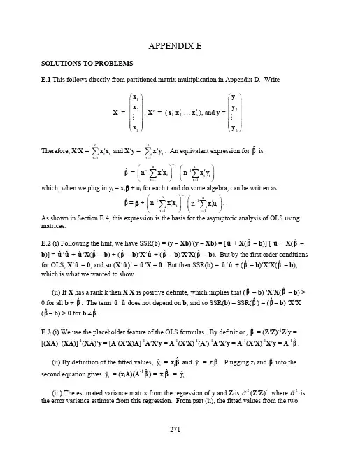
271APPENDIX ESOLUTIONS TO PROBLEMSE.1 This follows directly from partitioned matrix multiplication in Appendix D. WriteX = 12n ⎛⎫ ⎪ ⎪ ⎪ ⎪ ⎪⎝⎭x x x , X ' = (1'x 2'x n 'x ), and y = 12n ⎛⎫ ⎪ ⎪ ⎪ ⎪ ⎪⎝⎭y y yTherefore, X 'X = 1nt t t ='∑x x and X 'y = 1nt t t ='∑x y . An equivalent expression for ˆβ isˆβ = 111nt t t n --=⎛⎫' ⎪⎝⎭∑x x 11n t t t n y -=⎛⎫' ⎪⎝⎭∑x which, when we plug in y t = x t β + u t for each t and do some algebra, can be written asˆβ= β + 111n t t t n --=⎛⎫' ⎪⎝⎭∑x x 11nt t t n u -=⎛⎫' ⎪⎝⎭∑x . As shown in Section E.4, this expression is the basis for the asymptotic analysis of OLS using matrices.E.2 (i) Following the hint, we have SSR(b ) = (y – Xb )'(y – Xb ) = [ˆu+ X (ˆβ – b )]'[ ˆu + X (ˆβ – b )] = ˆu'ˆu + ˆu 'X (ˆβ – b ) + (ˆβ – b )'X 'ˆu + (ˆβ – b )'X 'X (ˆβ – b ). But by the first order conditions for OLS, X 'ˆu= 0, and so (X 'ˆu )' = ˆu 'X = 0. But then SSR(b ) = ˆu 'ˆu + (ˆβ – b )'X 'X (ˆβ – b ), which is what we wanted to show.(ii) If X has a rank k then X 'X is positive definite, which implies that (ˆβ– b ) 'X 'X (ˆβ – b ) > 0 for all b ≠ ˆβ. The term ˆu 'ˆu does not depend on b , and so SSR(b ) – SSR(ˆβ) = (ˆβ– b ) 'X 'X (ˆβ– b ) > 0 for b ≠ˆβ.E.3 (i) We use the placeholder feature of the OLS formulas. By definition, β = (Z 'Z )-1Z 'y =[(XA )' (XA )]-1(XA )'y = [A '(X 'X )A ]-1A 'X 'y = A -1(X 'X )-1(A ')-1A 'X 'y = A -1(X 'X )-1X 'y = A -1ˆβ.(ii) By definition of the fitted values, ˆt y = ˆt x β and t y = tz β. Plugging z t and β into the second equation gives ty = (x t A )(A -1ˆβ) = ˆt x β = ˆty .(iii) The estimated variance matrix from the regression of y and Z is 2σ(Z 'Z )-1 where 2σ is the error variance estimate from this regression. From part (ii), the fitted values from the two272regressions are the same, which means the residuals must be the same for all t . (The dependentvariable is the same in both regressions.) Therefore, 2σ = 2ˆσ. Further, as we showed in part (i), (Z 'Z )-1 = A -1(X 'X )-1(A ')-1, and so 2σ(Z 'Z )-1 = 2ˆσA -1(X 'X )-1(A -1)', which is what we wanted to show.(iv) The j β are obtained from a regression of y on XA , where A is the k ⨯ k diagonal matrixwith 1, a 2, , a k down the diagonal. From part (i), β = A -1ˆβ. But A -1 is easily seen to be the k ⨯ k diagonal matrix with 1, 12a -, , 1k a - down its diagonal. Straightforward multiplicationshows that the first element of A -1ˆβis 1ˆβ and the j th element is ˆjβ/a j , j = 2, , k .(v) From part (iii), the estimated variance matrix of β is 2ˆσA -1(X 'X )-1(A -1)'. But A -1 is a symmetric, diagonal matrix, as described above. The estimated variance of j β is the j thdiagonal element of 2ˆσA -1(X 'X )-1A -1, which is easily seen to be = 2ˆσc jj /2ja -, where c jj is the j th diagonal element of (X 'X )-1. The square root of this, a j |, is se(j β), which is simply se(j β)/|a j |.(vi) The t statistic for j β is, as usual,j β/se(j β) = (ˆj β/a j )/[se(ˆjβ)/|a j |],and so the absolute value is (|ˆj β|/|a j |)/[se(ˆj β)/|a j |] = |ˆj β|/se(ˆjβ), which is just the absolute value of the t statistic for ˆjβ. If a j > 0, the t statistics themselves are identical; if a j < 0, the t statistics are simply opposite in sign.E.4 (i) 垐?E(|)E(|)E(|).====δX GβX G βX Gβδ(ii) 2121垐?Var(|)Var(|)[Var(|)][()][()].σσ--'''''====δX GβX G βX G G X X G G X X G(iii) The vector of regression coefficients from the regression y on XG -1 is111111111111[()]()[()]() ()[()]()ˆ ()()().------------''''''='''''=''''''''===XG XG XG y G X XG G X y G X X G G X yG X X G G X y G X X X y δFurther, as shown in Problem E.3, the residuals are the same as from the regression y on X , andso the error variance estimate, 2ˆ,σis the same. Therefore, the estimated variance matrix is。

伍德⾥奇---计量经济学第2章部分计算机习题详解（MATLAB）班级：⾦融学×××班姓名：××学号：×××××××C2.1 401K.RAW prate=β0+β1mrate解：（ⅰ）求出计划的样本中平均参与率和平均匹配率.所以，平均参与率为87.36，平均匹配率为0.73.（ⅱ）报告结果以及样本容量和R2.β1=mrate i?mrate(prate i?prate)ni=1mrate i?mrate2ni=1=cov(x,y)var(x)β0=prate?β1mrate=A?β1B R2=SSESST所以β1= 5.8611;所以β0= 83.07.= 0.0747, n=1534.且R2=SSESST（ⅲ）解释⽅程中的截距和mrate的系数.⽅程中的截距β0意味着，当mrate= 0时，预测的参与率是83.07％。

⽽系数mrate意味着员⼯每投⼊⼀美元，prate的预期变化为5.86个百分点。

（ⅳ）当mrate=3.5时，求出prate的预测值。

只是⼀个合理的预测吗？解释这⾥出现的情况.由（ⅱ）可得prate=83.07+5.86mrate，所以当mrate=3.5时，prate= 83.07 + 5.86 * 3.5 = 103.58，即prate的预测值是103.85.这不是⼀个合理的预测，因为最多只可能有100％的参与率，不可能超过100% 。

(ⅴ)prate的变异中，有多少是由mrate解释的？这是⼀个⾜够⼤的量吗？在prate的变异中，有7.47% 是由mrate解释的,这不是⼀个⾜够⼤的量，意味着还有许多其他因素影响计划的参与率。

C2.2 CEOSAL2.RAW lo g salary=β0+β1ceoten+u解：（ⅰ）求出样本中的平均年薪和平均任期.所以，平均年薪为865.86，平均任期为7.95.（ⅱ）有多少位CEO尚处于担任CEO的第⼀年（即ceoten=0）?最长的CEO任期是多少？所以，有5位CEO尚处于担任CEO的第⼀年；所以，最长的CEO任期是37年。

第二篇时间序列数据的回归分析第10章时间序列数据的基本回归分析10.1 复习笔记考点一：时间序列数据★★1．时间序列数据与横截面数据的区别（1）时间序列数据集是按照时间顺序排列。

（2）时间序列数据与横截面数据被视为随机结果的原因不同。

（3）一个时间序列过程的所有可能的实现集，便相当于横截面分析中的总体。

时间序列数据集的样本容量就是所观察变量的时期数。

2．时间序列模型的主要类型（见表10-1）表10-1 时间序列模型的主要类型考点二：经典假设下OLS的有限样本性质★★★★1．高斯-马尔可夫定理假设（见表10-2）表10-2 高斯-马尔可夫定理假设2．OLS估计量的性质与高斯-马尔可夫定理（见表10-3）表10-3 OLS估计量的性质与高斯-马尔可夫定理3．经典线性模型假定下的推断（1）假定TS.6（正态性）假定误差u t独立于X，且具有独立同分布Normal（0，σ2）。

该假定蕴涵了假定TS.3、TS.4和TS.5，但它更强，因为它还假定了独立性和正态性。

（2）定理10.5（正态抽样分布）在时间序列的CLM假定TS.1～TS.6下，以X为条件，OLS估计量遵循正态分布。

而且，在虚拟假设下，每个t统计量服从t分布，F统计量服从F分布，通常构造的置信区间也是确当的。

定理10.5意味着，当假定TS.1～TS.6成立时，横截面回归估计与推断的全部结论都可以直接应用到时间序列回归中。

这样t统计量可以用来检验个别解释变量的统计显著性，F统计量可以用来检验联合显著性。

考点三：时间序列的应用★★★★★1．函数形式、虚拟变量除了常见的线性函数形式，其他函数形式也可以应用于时间序列中。

最重要的是自然对数，在应用研究中经常出现具有恒定百分比效应的时间序列回归。

虚拟变量也可以应用在时间序列的回归中，如某一期的数据出现系统差别时，可以采用虚拟变量的形式。

2．趋势和季节性（1）描述有趋势的时间序列的方法（见表10-4）表10-4 描述有趋势的时间序列的方法（2）回归中的趋势变量由于某些无法观测的趋势因素可能同时影响被解释变量与解释变量，被解释变量与解释变量均随时间变化而变化，容易得到被解释变量与解释变量之间趋势变量的关系，而非真正的相关关系，导致了伪回归。

伍德⾥奇《计量经济学导论》（第6版）复习笔记和课后习题详解-多元回归分析：推断【圣才出品】第4章多元回归分析：推断4.1复习笔记考点⼀：OLS估计量的抽样分布★★★1．假定MLR.6（正态性）假定总体误差项u独⽴于所有解释变量，且服从均值为零和⽅差为σ2的正态分布，即：u～Normal（0，σ2）。

对于横截⾯回归中的应⽤来说，假定MLR.1～MLR.6被称为经典线性模型假定。

假定下对应的模型称为经典线性模型（CLM）。

2．⽤中⼼极限定理（CLT）在样本量较⼤时，u近似服从于正态分布。

正态分布的近似效果取决于u中包含多少因素以及因素分布的差异。

但是CLT的前提假定是所有不可观测的因素都以独⽴可加的⽅式影响Y。

当u是关于不可观测因素的⼀个复杂函数时，CLT论证可能并不适⽤。

3．OLS估计量的正态抽样分布定理4.1（正态抽样分布）：在CLM假定MLR.1～MLR.6下，以⾃变量的样本值为条件，有：∧βj～Normal（βj，Var（∧βj））。

将正态分布函数标准化可得：（∧βj－βj）/sd（∧βj）～Normal（0，1）。

注：∧β1，∧β2，…，∧βk的任何线性组合也都符合正态分布，且∧βj的任何⼀个⼦集也都具有⼀个联合正态分布。

考点⼆：单个总体参数检验：t检验★★★★1．总体回归函数总体模型的形式为：y＝β0＋β1x1＋…＋βk x k＋u。

假定该模型满⾜CLM假定，βj的OLS 量是⽆偏的。

2．定理4.2：标准化估计量的t分布在CLM假定MLR.1～MLR.6下，（∧βj－βj）/se（∧βj）～t n－k－1，其中，k＋1是总体模型中未知参数的个数（即k个斜率参数和截距β0）。

t统计量服从t分布⽽不是标准正态分布的原因是se（∧βj）中的常数σ已经被随机变量∧σ所取代。

t统计量的计算公式可写成标准正态随机变量（∧βj－βj）/sd（∧βj）与∧σ2/σ2的平⽅根之⽐，可以证明⼆者是独⽴的；⽽且（n－k－1）∧σ2/σ2～χ2n－k－1。

4
Ramsey’s RESET
RESET relies on a trick similar to the special form of the White test Instead of adding functions of the x’s directly, we add and test functions of ŷ So, estimate y = b0 + b1x1 + … + bkxk + d1ŷ2 + d1ŷ3 +error and test H0: d1 = 0, d2 = 0 using F~F2,n-k-3 or LM~χ22
8
Proxy Variables (continued)
What do we need for for this solution to give us consistent estimates of b1 and b2? E(x3* | x1, x2, x3) = E(x3* | x3) = d0 + d3x3 That is, u is uncorrelated with x1, x2 and x3* and v3 is uncorrelated with x1, x2 and x3 So really running y = (b0 + b3d0) + b1x1+ b2x2 + b3d3x3 + (u + b3v3) and have just redefined intercept, error term x3 coefficient
5
Nonnested Alternative Tests
If the models have the same dependent variables, but nonnested x’s could still just make a giant model with the x’s from both and test joint exclusion restrictions that lead to one model or the other An alternative, the Davidson-MacKinnon test, uses ŷ from one model as regressor in the second model and tests for significance

计量经济学第六版第二章计算机课后答案1．计量经济学是一门什么样的学科？答：计量经济学的英文单词是Econometrics，本意是“经济计量”，研究经济问题的计量方法，因此有时也译为“经济计量学”。

将Econometrics译为“计量经济学”是为了强调它是现代经济学的一门分支学科，不仅要研究经济问题的计量方法，还要研究经济问题发展变化的数量规律。

可以认为，计量经济学是以经济理论为指导，以经济数据为依据，以数学、统计方法为手段，通过建立、估计、检验经济模型，揭示客观经济活动中存在的随机因果关系的一门应用经济学的分支学科。

2．计量经济学与经济理论、数学、统计学的联系和区别是什么？答：计量经济学是经济理论、数学、统计学的结合，是经济学、数学、统计学的交叉学科（或边缘学科）。

计量经济学与经济学、数学、统计学的联系主要是计量经济学对这些学科的应用。

计量经济学对经济学的应用主要体现在以下几个方面：第一，计量经济学模型的选择和确定，包括对变量和经济模型的选择，需要经济学理论提供依据和思路；第二，计量经济分析中对经济模型的修改和调整，如改变函数形式、增减变量等，需要有经济理论的指导和把握；第三，计量经济分析结果的解读和应用也需要经济理论提供基础、背景和思路。

计量经济学对统计学的应用，至少有两个重要方面：一是计量经济分析所采用的数据的收集与处理、参数的估计等，需要使用统计学的方法和技术来完成；一是参数估计值、模型的预测结果的可靠性，需要使用统计方法加以分析、判断。

计量经济学对数学的应用也是多方面的，首先，对非线性函数进行线性转化的方法和技巧，是数学在计量经济学中的应用；其次，任何的参数估计归根结底都是数学运算，较复杂的参数估计方法，或者较复杂的模型的参数估计，更需要相当的数学知识和数学运算能力，另外，在计量经济理论和方法的研究方面，需要用到许多的数学知识和原理。

计量经济学与经济学、数学、统计学的区别也很明显，经济学、数学、统计学中的任何一门学科，都不能替代计量经济学，这三门学科简单地合起来，也不能替代计量经济学。

第9章模型设定和数据问题的深入探讨9.1复习笔记考点一：函数形式设误检验（见表9-1）★★★★表9-1函数形式设误检验考点二：对无法观测解释变量使用代理变量★★★1．代理变量代理变量就是某种与分析中试图控制而又无法观测的变量相关的变量。

（1）遗漏变量问题的植入解假设在有3个自变量的模型中，其中有两个自变量是可以观测的，解释变量x3*观测不到：y＝β0＋β1x1＋β2x2＋β3x3*＋u。

但有x3*的一个代理变量，即x3，有x3*＝δ0＋δ3x3＋v3。

其中，x3*和x3正相关，所以δ3＞0；截距δ0容许x3*和x3以不同的尺度来度量。

假设x3就是x3*，做y对x1，x2，x3的回归，从而利用x3得到β1和β2的无偏（或至少是一致）估计量。

在做OLS之前，只是用x3取代了x3*，所以称之为遗漏变量问题的植入解。

代理变量也可以以二值信息的形式出现。

（2）植入解能得到一致估计量所需的假定（见表9-2）表9-2植入解能得到一致估计量所需的假定2．用滞后因变量作为代理变量对于想要控制无法观测的因素，可以选择滞后因变量作为代理变量，这种方法适用于政策分析。

但是现期的差异很难用其他方法解释。

使用滞后被解释变量不是控制遗漏变量的唯一方法，但是这种方法适用于估计政策变量。

考点三：随机斜率模型★★★1．随机斜率模型的定义如果一个变量的偏效应取决于那些随着总体单位的不同而不同的无法观测因素，且只有一个解释变量x，就可以把这个一般模型写成：y i＝a i＋b i x i。

上式中的模型有时被称为随机系数模型或随机斜率模型。

对于上式模型，记a i＝a＋c i和b i＝β＋d i，则有E（c i）＝0和E（d i）＝0，代入模型得y i＝a＋βx i＋u i，其中，u i＝c i＋d i x i。

2．保证OLS无偏（一致性）的条件（1）简单回归当u i＝c i＋d i x i时，无偏的充分条件就是E（c i｜x i）＝E（c i）＝0和E（d i｜x i）＝E（d i）＝0。

第14章高级面板数据方法14.1复习笔记考点一：固定效应估计法★★★★★1．固定效应变换固定效应变换又称组内变换，考虑仅有一个解释变量的模型：对每个i，有y it ＝β1x it ＋a i ＋u it ，t＝1，2，…，T对每个i 求方程在时间上的平均，便得到＿y i ＝β1＿x i ＋a i ＋＿u i 其中，11T it t y T y-==∑（关于时间的均值）。

因为a i 在不同时间固定不变，故它会在原模型和均值模型中都出现，如果对于每个t，两式相减，便得到y it －＿y i ＝β1（x it －＿x i ）＋u it －＿u i ，t＝1，2，…，T或1 12it it it y x u ,t ,,,T=+=&&&&&&L β其中，it it i y y y =-&&是y 的除时间均值数据；对it x &&和it u &&的解释也类似。

方程的要点在于，非观测效应a i 已随之消失，从而可以使用混合OLS 去估计式1 12it it it y x u ,t ,,,T =+=&&&&&&L β。

上式的混合OLS 估计量被称为固定效应估计量或组内估计量。

组间估计量可以从横截面方程＿y i ＝β1＿x i ＋a i ＋＿u i 的OLS 估计量而得到，即同时使用y 和x的时间平均值做一个横截面回归。

如果a i与＿x i相关，估计量是有偏误的。

而如果认为a i 与x it无关，则使用随机效应估计量要更好。

组间估计量忽视了变量如何随着时间而变化。

在方程中添加更多解释变量不会引起什么变化。

2．固定效应模型（1）无偏性原始的非固定效应模型，只要让每一个变量都减去时间均值数据，即可得到固定效应模型。

固定效应模型的无偏性是建立在严格外生性的假定下的，所以FE模型需要假定特异误差u it应与所有时期的每个解释变量都无关。

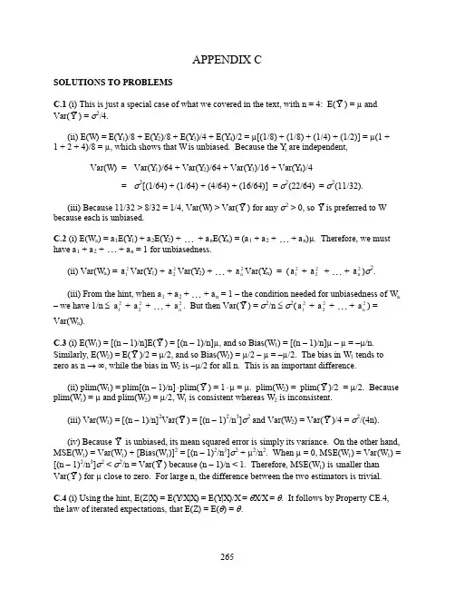
265APPENDIX CSOLUTIONS TO PROBLEMSC.1 (i) This is just a special case of what we covered in the text, with n = 4: E(Y ) = µ and Var(Y ) = σ2/4.(ii) E(W ) = E(Y 1)/8 + E(Y 2)/8 + E(Y 3)/4 + E(Y 4)/2 = µ[(1/8) + (1/8) + (1/4) + (1/2)] = µ(1 + 1 + 2 + 4)/8 = µ, which shows that W is unbiased. Because the Y i are independent, Var(W ) = Var(Y 1)/64 + Var(Y 2)/64 + Var(Y 3)/16 + Var(Y 4)/4 = σ2[(1/64) + (1/64) + (4/64) + (16/64)] = σ2(22/64) = σ2(11/32).(iii) Because 11/32 > 8/32 = 1/4, Var(W ) > Var(Y ) for any σ2 > 0, so Y is preferred to W because each is unbiased.C.2 (i) E(W a ) = a 1E(Y 1) + a 2E(Y 2) + + a n E(Y n ) = (a 1 + a 2 + + a n )µ. Therefore, we must have a 1 + a 2 + + a n = 1 for unbiasedness.(ii) Var(W a ) = 21a Var(Y 1) + 22a Var(Y 2) + + 2n a Var(Y n ) = (21a + 22a+ + 2n a )σ2.(iii) From the hint, when a 1 + a 2 + + a n = 1 – the condition needed for unbiasedness of W a– we have 1/n ≤ 21a + 22a + + 2n a . But then Var(Y ) = σ2/n ≤ σ2(21a+ 22a + + 2n a ) =Var(W a ).C.3 (i) E(W 1) = [(n – 1)/n ]E(Y ) = [(n – 1)/n ]µ, and so Bias(W 1) = [(n – 1)/n ]µ – µ = –µ/n . Similarly, E(W 2) = E(Y )/2 = µ/2, and so Bias(W 2) = µ/2 – µ = –µ/2. The bias in W 1 tends to zero as n → ∞, while the bias in W 2 is –µ/2 for all n . This is an important difference.(ii) plim(W 1) = plim[(n – 1)/n ]⋅plim(Y ) = 1⋅µ = µ. plim(W 2) = plim(Y )/2 = µ/2. Because plim(W 1) = µ and plim(W 2) = µ/2, W 1 is consistent whereas W 2 is inconsistent.(iii) Var(W 1) = [(n – 1)/n ]2Var(Y ) = [(n – 1)2/n 3]σ2 and Var(W 2) = Var(Y )/4 = σ2/(4n ).(iv) Because Y is unbiased, its mean squared error is simply its variance. On the other hand, MSE(W 1) = Var(W 1) + [Bias(W 1)]2 = [(n – 1)2/n 3]σ2 + µ2/n 2. When µ = 0, MSE(W 1) = Var(W 1) = [(n – 1)2/n 3]σ2 < σ2/n = Var(Y ) because (n – 1)/n < 1. Therefore, MSE(W 1) is smaller than Var(Y ) for µ close to zero. For large n , the difference between the two estimators is trivial.C.4 (i) Using the hint, E(Z |X ) = E(Y /X |X ) = E(Y |X )/X = θX /X = θ. It follows by Property CE.4, the law of iterated expectations, that E(Z ) = E(θ) = θ.266(ii) This follows from part (i) and the fact that the sample average is unbiased for the population average: write11111(/),n niiii i W nY X n Z --====∑∑where Z i = Y i /X i . From part (i), E(Z i ) = θ for all i .(iii) In general, the average of the ratios, Y i /X i , is not the ratio of averages, 2/.W Y X = (This non-equivalence is discussed a bit on page 676.) Nevertheless, W 2 is also unbiased, as a simple application of the law of iterated expectations shows. First, E(Y i |X 1,…,X n ) = E(Y i |X i ) under random sampling because the observations are independent. Therefore, E(Y i |X 1,…,X n ) = i X θ and so11111111E(|,...,)E(|,...,).nnn inii i ni i Y X X nY X XnXn X X θθθ--==-=====∑∑∑Therefore, 211E(|,...,)E(/|,...,)/,n n W X X Y X X X X X θθ===which means that W 2 is actually unbiased conditional on 1(,...,)n X X , and therefore also unconditionally unbiased.(iv) For the n = 17 observations given in the table – which are, incidentally, the first 17observations in the file CORN.RAW – the point estimates are w 1 = .418 and w 2 = 120.43/297.41 = .405. These are pretty similar estimates. If we use w 1, we estimate E(Y |X = x ) for any x > 0 asE(|)Y X x = = .418 x . For example, if x = 300 then the predicted yield is .418(300) = 125.4.C.5 (i) While the expected value of the numerator of G is E(Y ) = θ, and the expected value of the denominator is E(1 – Y ) = 1 – θ, the expected value of the ratio is not the ratio of the expected value.(ii) By Property PLIM.2(iii), the plim of the ratio is the ratio of the plims (provided the plim of the denominator is not zero): plim(G ) = plim[Y /(1 – Y )] = plim(Y )/[1 – plim(Y )] = θ/(1 – θ) = γ.C.6 (i) H 0: µ = 0.(ii) H 1: µ < 0.(iii) The standard error of yis s ≈ 15.55. Therefore, the t statistic for testing H 0: µ = 0 is t = y /se(y ) = –32.8/15.55 ≈ –2.11. We obtain the p -value as P(Z ≤ –2.11), where Z ~ Normal(0,1). These probabilities are in Table G.1: p -value = .0174. Because the p -。

伍德里奇计量经济学第六版答案AppendixBAPPENDIX BSOLUTIONS TO PROBLEMSB.1 Before the student takes the SAT exam, we do not know – nor can we predict with certainty – what the score will be. The actual score depends on numerous factors, many of which we cannot even list, let alone know ahead of time. (The student’s innate abil ity, how the student feels on exam day, and which particular questions were asked, are just a few.) The eventual SAT score clearly satisfies the requirements of a random variable.B.2 (i) P(X≤ 6) = P[(X–5)/2 ≤ (6 –5)/2] = P(Z≤ .5) ≈.692, where Z denotes a Normal (0,1) random variable. [We obtain P(Z≤ .5) from Table G.1.](ii) P(X > 4) = P[(X– 5)/2 > (4 – 5)/2] = P(Z > -.5) = P(Z≤ .5) ≈ .692.(iii) P(|X– 5| > 1) = P(X– 5 > 1) + P(X– 5 < –1) = P(X > 6) + P(X < 4) ≈ (1 – .692) + (1 – .692) = .616, where we have used answers from parts (i) and (ii).B.3 (i) Let Y it be the binary variable equal to one if fund i outperforms the market in year t. By assumption, P(Y it = 1) = .5 (a 50-50 chance of outperforming the market for each fund in each year). Now, for any fund, we are also assuming that performance relative to the market is independent across years. But then the probability that fund i outperforms the market in all 10 years, P(Y i1 = 1,Y i2 = 1, , Y i,10 = 1), is just the product of the probabilities: P(Y i1 = 1)?P(Y i2 = 1) P(Y i,10 = 1) = (.5)10 = 1/1024 (which is slightly less than .001). In fact, if we define a binary random variable Y i such that Y i = 1 if and only if fund i outperformed the market in all 10 years, then P(Y i = 1) = 1/1024.(ii) Let X denote the number of funds out of 4,170 that outperform the market in all 10 years. Then X = Y1 + Y2 + + Y4,170. If we assume that performance relative to the market is independent across funds, then X has the Binomial (n,θ) distribution with n = 4,170 and θ =1/1024. We want to compute P(X≥ 1) = 1 – P(X = 0) = 1 –P(Y1 = 0, Y2= 0, …, Y4,170 = 0) = 1 –P(Y1 = 0)? P(Y2 = 0)P(Y4,170 = 0) = 1 –(1023/1024)4170≈.983. This means, if performance relative to the market is random and independent across funds, it is almost certain that at least one fund will outperform the market in all 10 years.(iii) Using the Stata command Binomial(4170,5,1/1024), the answer is about .385. So there is a nontrivial chance that at least five funds will outperform the market in all 10 years.B.4 We want P(X ≥.6). Because X is continuous, this is the same as P(X > .6) = 1 –P(X≤ .6) =F(.6) = 3(.6)2– 2(.6)3 = .648. One way to interpret this is that almost 65% of all counties havean elderly employment rate of .6 or higher.B.5 (i) As stated in the hint, if X is the number of jurors convinced of Simpson’s innocence, then X ~ Binomial(12,.20). We want P(X≥ 1) = 1 – P(X = 0) = 1 –(.8)12≈ .931.263264 (ii) Above, we computed P(X = 0) as about .069. We need P(X = 1), which we obtain from(B.14) with n = 12, θ = .2, and x = 1: P(X = 1) = 12? (.2)(.8)11 ≈ .206. Therefore, P(X ≥ 2) ≈ 1 – (.069 + .206) = .725, so there is almost a three in four chance that the jury had at least two members convinced of Simpson’s innocence prior to the trial.B.6 E(X ) = 30()xf x dx ? = 320[(1/9)] x x dx ? = (1/9) 330x dx ?.But 330x dx ? = (1/4)x 430| = 81/4. Therefore, E(X ) = (1/9)(81/4) = 9/4, or 2.25 years.B.7 In eight attempts the expected number of free throws is 8(.74) = 5.92, or about six free throws.B.8 The weights for the two-, three-, and four-credit courses are 2/9, 3/9, and 4/9, respectively. Let Y j be the grade in the j th course, j = 1, 2, and 3, and let X be the overall grade point average. Then X = (2/9)Y 1 + (3/9)Y 2 + (4/9)Y 3 and the expected value is E(X ) = (2/9)E(Y 1) + (3/9)E(Y 2) + (4/9)E(Y 3) = (2/9)(3.5) + (3/9)(3.0) + (4/9)(3.0) = (7 + 9 + 12)/9 ≈ 3.11.B.9 If Y is salary in dollars then Y = 1000?X , and so the expected value of Y is 1,000 times the expected value of X , and the standard deviation of Y is 1,000 times the standard deviation of X . Therefore, the expected value and standard deviation of salary, measured in dollars, are $52,300 and $14,600, respectively.B.10 (i) E(GPA |SAT = 800) = .70 + .002(800) = 2.3. Similarly, E(GPA |SAT =1,400) = .70 + .002(1400) = 3.5. The difference in expected GPAs is substantial, but the difference in SAT scores is also rather large.(ii) Following the hint, we use the law of iterated expectations. SinceE(GPA |SAT ) = .70 + .002 SAT , the (unconditional) expected value of GPA is .70 + .002 E(SAT ) = .70 + .002(1100) = 2.9.。

计量经济学导论(伍德里奇)第二章课后作业.txt明骚易躲，暗贱难防。

佛祖曰：你俩就是大傻B！当白天又一次把黑夜按翻在床上的时候，太阳就出生了*用STATA做的*文件位置："E:\teaching*做do文件doeditcd "E:\teaching"*练习2.3 录入8名学生的ACT分数和GPA（平均积分点）input id GPA ACT1 2.8 212 3.4 243 3.0 264 3.5 275 3.6 296 3.0 257 2.7 258 3.7 30endsave zhangwenwen*回归分析reg GPA ACT,r*方程的斜率为 0.1021978，截距为 0.5681319.display _b[_cons]+_b[ACT]*20*当ACT=20时，GPA的预测值为 2.6120879.*练习2.4use BWGHT.dta , clearreg bwght cigs , rdisplay _b[_cons]+_b[cigs]*0*当吸烟数为0时，婴儿出生时的体重预测值为119.7719盎司。

display _b[_cons]+_b[cigs]*20*当吸烟数为0时，婴儿出生时的体重预测值为109.4965盎司。

*bwght=119.77-0.514cigs 从这个回归中可以得到婴儿出生体重和母亲吸烟习惯之间的关系.*母亲在怀孕期间平均每天的吸烟数增加一个单位，婴儿的体重下降0.514盎司。

*练习2.10use 401K.DTA,clearsum*计划样中平均参与率是87.36291，平均匹配率是0.7315124*下面做回归分析regress prate mrate,robust*Estimated slope（样本斜率） = 5.861079*Estimated intercept（截距） = 83.07546,*Estimated regression line: prate = 83.075+5.861mrate*样本容量是1534，R-平方=0.0747*如果mrate=0,那么参与率就是83.0754%。

2.10(iii) From (2.57), Var(1ˆβ) = σ2/21()n i i x x =⎛⎫- ⎪⎝⎭∑. 由提示：： 21n ii x =∑ ≥ 21()n i i x x =-∑, and so Var(1β) ≤ Var(1ˆβ). A more direct way to see this is to write(一个更直接的方式看到这是编写) 21()ni i x x =-∑ = 221()n i i x n x =-∑, which is less than21n i i x=∑unless x = 0.(iv)给定的c 2i x 但随着x 的增加， 1ˆβ的方差与Var(1β)的相关性也增加.0β小时1β的偏差也小.因此, 在均方误差的基础上不管我们选择0β还是1β要取决于0β,x ,和n 的大小 (除了 21n i i x=∑的大小).3.7We can use Table 3.2. By definition, 2β > 0, and by assumption, Corr(x 1,x 2) < 0. Therefore, there is a negative bias in 1β: E(1β) < 1β. This means that, on average across different random samples, the simpleregression estimator underestimates the effect of the training program. It is even possible that E(1β) isnegative even though 1β > 0. 我们可以使用表3.2。

根据定义，> 0，由假设，科尔（X1，X2）<0。

因此，有一个负偏压为：E （）<。

这意味着，平均在不同的随机抽样，简单的回归估计低估的培训计划的效果。

CHAPTER 2TEACHING NOTESThis is the chapter where I expect students to follow most, if not all, of the algebraic derivations. In class I like to derive at least the unbiasedness of the OLS slope coefficient, and usually I derive the variance. At a minimum, I talk about the factors affecting the variance. To simplify the notation, after I emphasize the assumptions in the population model, and assume random sampling, I just condition on the values of the explanatory variables in the sample. Technically, this is justified by random sampling because, for example, E(u i|x1,x2,…,x n) = E(u i|x i) by independent sampling. I find that students are able to focus on the key assumption SLR.4 and subsequently take my word about how conditioning on the independent variables in the sample is harmless. (If you prefer, the appendix to Chapter 3 does the conditioning argument carefully.) Because statistical inference is no more difficult in multiple regression than in simple regression, I postpone inference until Chapter 4. (This reduces redundancy and allows you to focus on the interpretive differences between simple and multiple regression.)You might notice how, compared with most other texts, I use relatively few assumptions to derive the unbiasedness of the OLS slope estimator, followed by the formula for its variance. This is because I do not introduce redundant or unnecessary assumptions. For example, once SLR.4 is assumed, nothing further about the relationship between u and x is needed to obtain the unbiasedness of OLS under random sampling.Incidentally, one of the uncomfortable facts about finite-sample analysis is that there is a difference between an estimator that is unbiased conditional on the outcome of the covariates and one that is unconditionally unbiased. If the distribution of the x i is such that they can all equal the same value with positive probability – as is the case with discreteness in the distribution –then the unconditional expectation does not really exist. Or, if it is made to exist then the estimator is not unbiased. I do not try to explain these subtleties in an introductory course, but I have had instructors ask me about the difference.SOLUTIONS TO PROBLEMS2.1 (i) Income, age, and family background (such as number of siblings) are just a fewpossibilities. It seems that each of these could be correlated with years of education. (Income and education are probably positively correlated; age and education may be negatively correlated because women in more recent cohorts have, on average, more education; and number of siblings and education are probably negatively correlated.)(ii) Not if the factors we listed in part (i) are correlated with educ . Because we would like to hold these factors fixed, they are part of the error term. But if u is correlated with educ then E(u|educ ) ≠ 0, and so SLR.4 fails.2.2 In the equation y = β0 + β1x + u , add and subtract α0 from the right hand side to get y = (α0 + β0) + β1x + (u - α0). Call the new error e = u - α0, so that E(e ) = 0. The new intercept is α0 + β0, but the slope is still β1.2.3 (i) Let y i = GPA i , x i = ACT i , and n = 8. Then x = 25.875, y =3.2125, 1ni =∑(x i – x )(y i – y ) =5.8125, and 1ni =∑(x i – x )2 = 56.875. From equation (2.9), we obtain the slope as 1ˆβ= 5.8125/56.875 ≈ .1022, rounded to four places after the decimal. From (2.17), 0ˆβ = y – 1ˆβx ≈ 3.2125 – (.1022)25.875 ≈ .5681. So we can writeGPA = .5681 + .1022 ACTn = 8.The intercept does not have a useful interpretation because ACT is not close to zero for the population of interest. If ACT is 5 points higher, GPA increases by .1022(5) = .511.(ii) The fitted values and residuals — rounded to four decimal places — are given along with the observation number i and GPA in the following table:You can verify that the residuals, as reported in the table, sum to -.0002, which is pretty close to zero given the inherent rounding error.(iii) When ACT = 20, GPA = .5681 + .1022(20) ≈ 2.61.(iv) The sum of squared residuals,21ˆni i u=∑, is about .4347 (rounded to four decimal places), and the total sum of squares,1ni =∑(y i – y )2, is about 1.0288. So the R -squared from the regressionisR 2 = 1 – SSR/SST ≈ 1 – (.4347/1.0288) ≈ .577.Therefore, about 57.7% of the variation in GPA is explained by ACT in this small sample of students.2.4 (i) When cigs = 0, predicted birth weight is 119.77 ounces. When cigs = 20, bwght = 109.49. This is about an 8.6% drop.(ii) Not necessarily. There are many other factors that can affect birth weight, particularly overall health of the mother and quality of prenatal care. These could be correlated withcigarette smoking during birth. Also, something such as caffeine consumption can affect birth weight, and might also be correlated with cigarette smoking.(iii) If we want a predicted bwght of 125, then cigs = (125 – 119.77)/( –.524) ≈–10.18, or about –10 cigarettes! This is nonsense, of course, and it shows what happens when we are trying to predict something as complicated as birth weight with only a single explanatory variable. The largest predicted birth weight is necessarily 119.77. Yet almost 700 of the births in the sample had a birth weight higher than 119.77.(iv) 1,176 out of 1,388 women did not smoke while pregnant, or about 84.7%. Because we are using only cigs to explain birth weight, we have only one predicted birth weight at cigs = 0. The predicted birth weight is necessarily roughly in the middle of the observed birth weights at cigs = 0, and so we will under predict high birth rates.2.5 (i) The intercept implies that when inc = 0, cons is predicted to be negative $124.84. This, of course, cannot be true, and reflects that fact that this consumption function might be a poor predictor of consumption at very low-income levels. On the other hand, on an annual basis, $124.84 is not so far from zero.(ii) Just plug 30,000 into the equation: cons = –124.84 + .853(30,000) = 25,465.16 dollars.(iii) The MPC and the APC are shown in the following graph. Even though the intercept is negative, the smallest APC in the sample is positive. The graph starts at an annual income level of $1,000 (in 1970 dollars).increases housing prices.(ii) If the city chose to locate the incinerator in an area away from more expensive neighborhoods, then log(dist) is positively correlated with housing quality. This would violate SLR.4, and OLS estimation is biased.(iii) Size of the house, number of bathrooms, size of the lot, age of the home, and quality of the neighborhood (including school quality), are just a handful of factors. As mentioned in part (ii), these could certainly be correlated with dist [and log(dist )].2.7 (i) When we condition on incbecomes a constant. So E(u |inc⋅e |inc) = ⋅E(e |inc⋅0 because E(e |inc ) = E(e ) = 0.(ii) Again, when we condition on incbecomes a constant. So Var(u |inc⋅e |inc2Var(e |inc ) = 2e σinc because Var(e |inc ) = 2e σ.(iii) Families with low incomes do not have much discretion about spending; typically, a low-income family must spend on food, clothing, housing, and other necessities. Higher income people have more discretion, and some might choose more consumption while others more saving. This discretion suggests wider variability in saving among higher income families.2.8 (i) From equation (2.66),1β = 1n i i i x y =⎛⎫ ⎪⎝⎭∑ / 21n i i x =⎛⎫ ⎪⎝⎭∑.Plugging in y i = β0 + β1x i + u i gives1β = 011()n i i i i x x u ββ=⎛⎫++ ⎪⎝⎭∑/ 21n i i x =⎛⎫ ⎪⎝⎭∑.After standard algebra, the numerator can be written as201111in n ni i i i i i x x x u ββ===++∑∑∑.Putting this over the denominator shows we can write 1β as1β = β01n i i x =⎛⎫ ⎪⎝⎭∑/ 21n i i x =⎛⎫ ⎪⎝⎭∑ + β1 + 1n i i i x u =⎛⎫ ⎪⎝⎭∑/ 21n i i x =⎛⎫⎪⎝⎭∑.Conditional on the x i , we haveE(1β) = β01n i i x =⎛⎫ ⎪⎝⎭∑/ 21n i i x =⎛⎫⎪⎝⎭∑ + β1because E(u i ) = 0 for all i . Therefore, the bias in 1β is given by the first term in this equation. This bias is obviously zero when β0 = 0. It is also zero when 1ni i x =∑ = 0, which is the same asx = 0. In the latter case, regression through the origin is identical to regression with an intercept. (ii) From the last expression for 1βin part (i) we have, conditional on the x i ,Var(1β) = 221n i i x -=⎛⎫ ⎪⎝⎭∑Var 1n i i i x u =⎛⎫ ⎪⎝⎭∑ = 221n i i x -=⎛⎫ ⎪⎝⎭∑21Var()n i i i x u =⎛⎫⎪⎝⎭∑= 221n i i x -=⎛⎫ ⎪⎝⎭∑221n i i x σ=⎛⎫ ⎪⎝⎭∑ = 2σ/ 21n i i x =⎛⎫ ⎪⎝⎭∑.(iii) From (2.57), Var(1ˆβ) = σ2/21()n i i x x =⎛⎫- ⎪⎝⎭∑. From the hint, 21n i i x =∑ ≥ 21()ni i x x =-∑, and so Var(1β) ≤ Var(1ˆβ). A more direct way to see this is to write 21()ni i x x =-∑ = 221()ni i x n x =-∑, which is less than 21ni i x =∑ unless x = 0.(iv) For a given sample size, the bias in 1β increases as x increases (holding the sum of the2ix fixed). But as x increases, the variance of 1ˆβincreases relative to Var(1β). The bias in 1β is also small when 0β is small. Therefore, whether we prefer 1β or 1ˆβ on a mean squared error basis depends on the sizes of 0β, x , and n (in addition to the size of 21ni i x =∑).2.9 (i) We follow the hint, noting that 1c y = 1c y (the sample average of 1i c y is c 1 times the sample average of y i ) and 2c x = 2c x . When we regress c 1y i on c 2x i (including an intercept) we use equation (2.19) to obtain the slope:2211121112222221111112221()()()()()()()()ˆ.()n ni iiii i nnii i i niii nii c x c x c y c y c c x x y y c x c x cx x x x y y c c c c x x ββ======----==----=⋅=-∑∑∑∑∑∑From (2.17), we obtain the intercept as 0β = (c 1y ) – 1β(c 2x ) = (c 1y ) – [(c 1/c 2)1ˆβ](c 2x ) = c 1(y – 1ˆβx ) = c 10ˆβ) because the intercept from regressing y i on x i is (y – 1ˆβx ).(ii) We use the same approach from part (i) along with the fact that 1()c y + = c 1 + y and2()c x + = c 2 + x . Therefore, 11()()i c y c y +-+ = (c 1 + y i ) – (c 1 + y ) = y i – y and (c 2 + x i ) – 2()c x + = x i – x . So c 1 and c 2 entirely drop out of the slope formula for the regression of (c 1 + y i )on (c 2 + x i ), and 1β = 1ˆβ. The intercept is 0β = 1()c y + – 1β2()c x + = (c 1 + y ) – 1ˆβ(c 2 + x ) = (1ˆy x β-) + c 1 – c 21ˆβ = 0ˆβ + c 1 – c 21ˆβ, which is what we wanted to show.(iii) We can simply apply part (ii) because 11log()log()log()i i c y c y =+. In other words, replace c 1 with log(c 1), y i with log(y i ), and set c 2 = 0.(iv) Again, we can apply part (ii) with c 1 = 0 and replacing c 2 with log(c 2) and x i with log(x i ). If 01垐 and ββ are the original intercept and slope, then 11ˆββ= and 0021垐log()c βββ=-.2.10 (i) This derivation is essentially done in equation (2.52), once (1/SST )x is brought inside the summation (which is valid because SST x does not depend on i ). Then, just define/SST i i x w d =.(ii) Because 111垐Cov(,)E[()] ,u u βββ=- we show that the latter is zero. But, from part (i),()1111ˆE[()] =E E().nn i i i i i i u wu u w u u ββ==⎡⎤-=⎢⎥⎣⎦∑∑ Because the i u are pairwise uncorrelated (they are independent), 22E()E(/)/i i u u u n n σ== (because E()0, i h u u i h =≠). Therefore,(iii) The formula for the OLS intercept is 0垐y x ββ=- and, plugging in 01y x u ββ=++ gives 01111垐?()().x u x u x βββββββ=++-=+--(iv) Because 1ˆ and u β are uncorrelated, 222222201垐Var()Var()Var()/(/SST )//SST x x u x n x n x ββσσσσ=+=+=+,which is what we wanted to show.(v) Using the hint and substitution gives ()220ˆVar()[SST /]/SST x xn x βσ=+ ()()2122221211/SST /SST .nni x i x i i n x x x n x σσ--==⎡⎤=-+=⎢⎥⎣⎦∑∑22111E()(/)(/)0.n n ni i i i i i i w u u w n n w σσ======∑∑∑2.11 (i) We would want to randomly assign the number of hours in the preparation course so that hours is independent of other factors that affect performance on the SAT. Then, we would collect information on SAT score for each student in the experiment, yielding a data set{(,):1,...,}i i sat hours i n =, where n is the number of students we can afford to have in the study. From equation (2.7), we should try to get as much variation in i hours as is feasible.(ii) Here are three factors: innate ability, family income, and general health on the day of the exam. If we think students with higher native intelligence think they do not need to prepare for the SAT, then ability and hours will be negatively correlated. Family income would probably be positively correlated with hours , because higher income families can more easily affordpreparation courses. Ruling out chronic health problems, health on the day of the exam should be roughly uncorrelated with hours spent in a preparation course.(iii) If preparation courses are effective,1β should be positive: other factors equal, an increase in hours should increase sat .(iv) The intercept, 0β, has a useful interpretation in this example: because E(u ) = 0, 0β is the average SAT score for students in the population with hours = 0.2.12 (i) I will show the result without using calculus. Let y ̅ be the sample average of the y i and write221122001112200112201()[()()]()2()()()()2()()()()()n niii i nnni i i i i nni i i i ni i y b y y y b y y y y y b y b y y y b y y n y b y y n y b ========-=-+-=-+--+-=-+--+-=-+-∑∑∑∑∑∑∑∑where we use the fact (see Appendix A) that 1()0ni i y y =-=∑ always. The first term does notdepend on 0b and the second term,20()n y b -, which is nonnegative, is clearly minimized when 0b y =.(ii) If we define i i u y y =-then 11()nni i i i u y y ===-∑∑and we already used the fact that this sumis zero in the proof in part (i).SOLUTIONS TO COMPUTER EXERCISESC2.1 (i) The average prate is about 87.36 and the average mrate is about .732.(ii) The estimated equation isprate= 83.05 + 5.86 mraten = 1,534, R2 = .075.(iii) The intercept implies that, even if mrate = 0, the predicted participation rate is 83.05 percent. The coefficient on mrate implies that a one-dollar increase in the match rate – a fairly large increase – is estimated to increase prate by 5.86 percentage points. This assumes, of course, that this change prate is possible (if, say, prate is already at 98, this interpretation makes no sense).(iv) If we plug mrate = 3.5 into the equation we get ˆprate= 83.05 + 5.86(3.5) = 103.59. This is impossible, as we can have at most a 100 percent participation rate. This illustrates that, especially when dependent variables are bounded, a simple regression model can give strange predictions for extreme values of the independent variable. (In the sample of 1,534 firms, only 34 have mrate≥ 3.5.)(v) mrate explains about 7.5% of the variation in prate. This is not much, and suggests that many other factors influence 401(k) plan participation rates.C2.2 (i) Average salary is about 865.864, which means $865,864 because salary is in thousands of dollars. Average ceoten is about 7.95.(ii) There are five CEOs with ceoten = 0. The longest tenure is 37 years.(iii) The estimated equation issalary= 6.51 + .0097 ceotenlog()n = 177, R2 = .013.We obtain the approximate percentage change in salary given ∆ceoten = 1 by multiplying the coefficient on ceoten by 100, 100(.0097) = .97%. Therefore, one more year as CEO is predicted to increase salary by almost 1%.C2.3 (i) The estimated equation issleep= 3,586.4 – .151 totwrkn = 706, R2 = .103.The intercept implies that the estimated amount of sleep per week for someone who does not work is 3,586.4 minutes, or about 59.77 hours. This comes to about 8.5 hours per night.(ii) If someone works two more hours per week then ∆totwrk = 120 (because totwrk ismeasured in minutes), and so sleep ∆= –.151(120) = –18.12 minutes. This is only a few minutes a night. If someone were to work one more hour on each of five working days, sleep ∆= –.151(300) = –45.3 minutes, or about five minutes a night.C2.4 (i) Average salary is about $957.95 and average IQ is about 101.28. The sample standard deviation of IQ is about 15.05, which is pretty close to the population value of 15.(ii) This calls for a level-level model: wage = 116.99 + 8.30 IQn = 935, R 2 = .096.An increase in IQ of 15 increases predicted monthly salary by 8.30(15) = $124.50 (in 1980 dollars). IQ score does not even explain 10% of the variation in wage .(iii) This calls for a log-level model:log()wage = 5.89 + .0088 IQ n = 935, R 2 = .099.If ∆IQ = 15 then log()wage ∆ = .0088(15) = .132, which is the (approximate) proportionate change in predicted wage. The percentage increase is therefore approximately 13.2.C2.5 (i) The constant elasticity model is a log-log model:log(rd ) = 0β + 1βlog(sales ) + u ,where 1β is the elasticity of rd with respect to sales .(ii) The estimated equation is log()rd = –4.105 + 1.076 log(sales )n = 32, R 2 = .910.The estimated elasticity of rd with respect to sales is 1.076, which is just above one. A one percent increase in sales is estimated to increase rd by about 1.08%.C2.6 (i) It seems plausible that another dollar of spending has a larger effect for low-spending schools than for high-spending schools. At low-spending schools, more money can go toward purchasing more books, computers, and for hiring better qualified teachers. At high levels of spending, we would expend little, if any, effect because the high-spending schools already have high-quality teachers, nice facilities, plenty of books, and so on.(ii) If we take changes, as usual, we obtain1110log()(/100)(%),math expend expend ββ∆=∆≈∆just as in the second row of Table 2.3. So, if %10,expend ∆=110/10.math β∆=(iii) The regression results are21069.34 11.16 log()408, .0297math expend n R =-+==(iv) If expend increases by 10 percent, 10math increases by about 1.1 percentage points. This is not a huge effect, but it is not trivial for low-spending schools, where a 10 percent increase in spending might be a fairly small dollar amount.(v) In this data set, the largest value of math10 is 66.7, which is not especially close to 100. In fact, the largest fitted values is only about 30.2.C2.7 (i) The average gift is about 7.44 Dutch guilders. Out of 4,268 respondents, 2,561 did not give a gift, or about 60 percent.(ii) The average mailings per year is about 2.05. The minimum value is .25 (which presumably means that someone has been on the mailing list for at least four years) and the maximum value is 3.5.(iii) The estimated equation is22.01 2.65 4,268, .0138gift mailsyear n R =+==(iv) The slope coefficient from part (iii) means that each mailing per year is associated with – perhaps even “causes” – an estimated 2.65 additional guilders, on average. Therefore, if each mailing costs one guilder, the expected profit from each mailing is estimated to be 1.65 guilders. This is only the average, however. Some mailings generate no contributions, or a contribution less than the mailing cost; other mailings generated much more than the mailing cost.(v) Because the smallest mailsyear in the sample is .25, the smallest predicted value of gifts is 2.01 + 2.65(.25) ≈ 2.67. Even if we look at the overall population, where some people have received no mailings, the smallest predicted value is about two. So, with this estimated equation, we never predict zero charitable gifts.C2.8 There is no “correct” answer to this question because all answers depend on how the random outcomes are generated. I used Stata 11 and, before generating the outcomes on the i x , I set the seed to the value 123. I reset the seed to 123 to generate the outcomes on the i u . Specifically, to answer parts (i) through (v), I used the sequence of commandsset obs 500set seed 123gen x = 10*runiform()sum xset seed 123gen u = 6*rnormal()sum ugen y = 1 + 2*x + ureg y xpredict uh, residgen x_uh = x*uhsum uh x_uhgen x_u = x*usum u x_u(i) The sample mean of the i x is about 4.912 with a sample standard deviation of about 2.874.(ii) The sample average of the i u is about .221, which is pretty far from zero. We do not get zero because this is just a sample of 500 from a population with a zero mean. The current sample is “unlucky” in the sense that the sample average is far from the population average. The sample standard deviation is about 5.768, which is nontrivially below 6, the population value.(iii) After generating the data on i y and running the regression, I get, rounding to three decimal places,0ˆ 1.862β= and 1ˆ 1.870β= The population values are 1 and 2, respectively. Thus, the estimated intercept based on this sample of data is well above the population value. The estimated slope is somewhat below the population value, 2. When we sample from a population our estimates contain sampling error; that is why the estimates differ from the population values.(iv) When I use the command sum uh x_uh and multiply by 500 I get, using scientific notation, sums equal to 4.181e-06 and .00003776, respectively. These are zero for practical purposes, and differ from zero only due to rounding inherent in the machine imprecision (which is unimportant).(v) We already computed the sample average of the i u in part (ii). When we multiply by 500 the sample average is about 110.74. The sum of i i x u is about 6.46. Neither is close to zero, and nothing says they should be particularly close.(vi) For this part I set the seed to 789. The sample average and standard deviation of the i x are about 5.030 and 2.913; those for the i u are about .077- and 5.979. When I generated the i y and run the regression I get0ˆ.701β= and 1ˆ 2.044β= These are different from those in part (iii) because they are obtained from a different random sample. Here, for both the intercept and slope, we get estimates that are much closer to the population values. Of course, in practice we would never know that.。

计量经济学导论第六版课后答案知识伍德里奇第一章：计量经济学介绍1. 为什么需要计量经济学？计量经济学的主要目标是提供一种科学的方法来解决经济问题。

经济学家需要使用数据来验证经济理论的有效性，并预测经济变量的发展趋势。

计量经济学提供了一种框架，使得经济学家能够使用数学和统计方法来分析经济问题。

2. 计量经济学的基本概念•因果推断：计量经济学的核心是通过观察数据来推断出变量之间的因果关系。

通过使用统计方法，我们可以分析出某个变量对另一个变量的影响。

•数据类型：计量经济学研究的数据可以是时间序列数据或截面数据。

时间序列数据是沿着时间轴观测到的数据，而截面数据是在某一时间点上观测到的数据。

•数据偏差：在计量经济学中，数据偏差是指由于样本选择问题、观测误差等原因导致数据与真实值之间的差异。

3. 计量经济学的方法计量经济学使用了许多统计和经济学方法来分析数据。

以下是一些常用的计量经济学方法：•最小二乘法（OLS）：在计量经济学中，最小二乘法是一种常用的回归方法。

它通过最小化观测值和预测值之间的平方差来估计未知参数。

•时间序列分析：时间序列分析是通过对时间序列数据进行模型化和预测来研究经济变量的变化趋势。

•面板数据分析：面板数据是同时包含时间序列和截面数据的数据集。

面板数据分析可以用于研究个体和时间的变化，以及它们之间的关系。

4. 计量经济学应用领域计量经济学广泛应用于经济学研究和实践中的各个领域。

以下是一些计量经济学的应用领域：•劳动经济学：计量经济学可以用来研究劳动力市场的供求关系、工资决定因素等问题。

•金融经济学：计量经济学可以用来研究证券价格、金融市场的波动等问题。

•产业组织经济学：计量经济学可以用来研究市场竞争、垄断力量等问题。

•发展经济学：计量经济学可以用来研究发展中国家的经济增长、贫困问题等。

第二章：统计学回顾1. 统计学基本概念•总体和样本：总体是指我们想要研究的全部个体或事物的集合，而样本是从总体中选取的一部分个体或事物。

第三篇高级专题第13章跨时横截面的混合：简单面板数据方法13.1复习笔记考点一：跨时独立横截面的混合★★★★★1．独立混合横截面数据的定义独立混合横截面数据是指在不同时点从一个大总体中随机抽样得到的随机样本。

这种数据的重要特征在于：都是由独立抽取的观测所构成的。

在保持其他条件不变时，该数据排除了不同观测误差项的相关性。

区别于单独的随机样本，当在不同时点上进行抽样时，样本的性质可能与时间相关，从而导致观测点不再是同分布的。

2．使用独立混合横截面的理由（见表13-1）表13-1使用独立混合横截面的理由3．对跨时结构性变化的邹至庄检验（1）用邹至庄检验来检验多元回归函数在两组数据之间是否存在差别（见表13-2）表13-2用邹至庄检验来检验多元回归函数在两组数据之间是否存在差别（2）对多个时期计算邹至庄检验统计量的办法①使用所有时期虚拟变量与一个（或几个、所有）解释变量的交互项，并检验这些交互项的联合显著性，一般总能检验斜率系数的恒定性。

②做一个容许不同时期有不同截距的混合回归来估计约束模型，得到SSR r。

然后，对T个时期都分别做一个回归，并得到相应的残差平方和，有：SSR ur＝SSR1＋SSR2＋…＋SSR T。

若有k个解释变量（不包括截距和时期虚拟变量）和T个时期，则需检验（T－1）k个约束。

而无约束模型中有T＋Tk个待估计参数。

所以，F检验的df为（T－1）k和n－T－Tk，其中n为总观测次数。

F统计量计算公式为：[（SSR r－SSR ur）/SSR ur][（n－T－Tk）/（Tk－k）]。

但该检验不能对异方差性保持稳健，为了得到异方差-稳健的检验，必须构造交互项并做一个混合回归。

4．利用混合横截面作政策分析（1）自然实验与真实实验当某些外生事件改变了个人、家庭、企业或城市运行的环境时，便产生了自然实验（准实验）。

一个自然实验总有一个不受政策变化影响的对照组和一个受政策变化影响的处理组。

自然实验中，政策发生后才能确定处理组和对照组。

品数（output）方面的信息。 （i）仔细陈述这个政策问题背后其他情况不变的思维试验。 （ii）一个企业培训其员工的决策看起来有可能独立于工人特征吗？工人可观测与不可
观测的特征各有哪些？ （iii）除工人特征之外，再列出一个影响工人生产力的因素。 （iv）你若发现 training 和 output 之间成正相关关系，你令人信服地证明了工作培训
2．工作培训项目的理由之一是能提高工人的生产力。假设要求你评估更多的工作培训 是否使工人更有生产力。不过，你没有工人的个人数据，而是有俄亥俄州制造企业的数据。 具体而言，对每个企业，你都有人均工作培训小时数（training）和单位工时生产的合格产
4 / 91
圣才电子书 十万种考研考证电子书、题库视频学习平台
十万种考研考证电子书、题库视频学习平台
表 1-1 经济数据的结构
2．面板数据与混合横截面数据的比较（见表 1-2） 表 1-2 面板数据与混合横截面数据的比较
2 / 91
圣才电子书 十万种考研考证电子书、题库视频学习平台

考点三：因果关系和其他条件不变 ★★
1．因果关系 因果关系是指一个变量的变动将引起另一个变量的变动，这是经济分析中的重要目标之 一。计量分析虽然能发现变量之间的相关关系，但是如果想要解释因果关系，还要排除模型 本身存在因果互逆的可能，否则很难让人信服。
答：讲不通。因为找出每周学习小时数（study）和每周工作小时数（work）之间的关 系，是说每周学习小时数（study）和每周工作小时数（work）之间有关系，但没有说是因 果关系，每周学习小时数可能与其他因素有关或每周工作小时数与其他因素有关。
4．对税收有控制权的州或省份有时候会减少税收来刺激经济增长。假设你被某州政府 雇佣来估计公司税率的影响，比如说对每单位州生产总值增长的影响。