Household Sample Surveys in Developing and Transition Countries

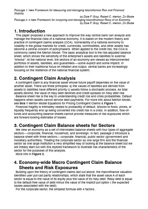
by Dale F. Gray, Robert C. Merton, Zvi Bodie 1.IntroductionThis paper proposes a new approach to improve the way central bank can analyze and manage the financial risks of a national economy. It is based on the modern theory and practice of contingent claims analysis (CCA). Vulnerability of a national economy to volatility in the global markets for credit, currencies, commodities, and other assets has become a central concern of policymakers. When applied to the credit risk, the CCA is commonly called the Merton Model. The basic analytical tool is the risk-adjusted balance sheet, which shows the sensitivity of the enterprise’s assets and liabilities to external “shocks”. At the national level, the sectors of an economy are viewed as interconnected portfolios of assets, liabilities, and guarantees----some explicit and some implicit. In addition to their traditional focus on inflation and output, central banks are increasingly focusing on the resilience of the national financial system.2.Contingent Claim AnalysisA contingent claim is any financial asset whose future payoff dependes on the value of another asset. There are three principles: a) the values of liabilities are derived from assets b) liabilities have different priority c) assets follow a stochastic process. As total assets decline, the value of risky debt declines and credit spreads on risky debt rise.Balance sheet risk is the key to understanding credit risk and crisis probabilities. Default happens when assets cannot service debt payments. For more info about Merton Model, see Box 1 Merton Model Equations for Pricing Contingent Claims & Figure 1.Financial fragility is intimately related to probability of default. Shocks to flows, prices, or liquidity frequently end up being converted into credit risk in a crisis. In addition, flow-of-funds and accounting balance sheets cannot provide measures of risk exposures which are forward-looking estimates of losses.3.Contingent Claim Balance sheets for SectorsWe view an economy as a set of interrelated balance sheets with four types of aggregate sectors----corporate, financial, household, and sovereign. In fact, passage 2 introduce a balance sheet with three sectors----corporate, financial, public sector (government and monetary authorities). Treating the corporate sector as one large firm and the financial sector as one large institution a very simplified way of looking at the balance sheet but we will initially start out with this stylized framework to illustrate risk characteristics of the sector for the purposes of this analysis.More info in Figure 2.4.Economy-wide Macro Contingent Claim BalanceSheets and Risk ExposuresBuilding upon the theory of contingent claims laid out above, the macrofinance valuation identities user put-call parity relationships, which state that the asset value A of each sector is equal to the value of its equity plus the value of its risky debt. Risky debt is equal to the default-free value of debt minus the value of the implicit put option ( the expected losses associated with the debt).For the corporate sector, the simplest formula with 4 factors.by Dale F. Gray, Robert C. Merton, Zvi Bodie For the financial sector, the support from government is added into its function with 4 factors.For the sovereign, passage 2 has more info. See in passage 2 Figure 2. Assets include: foreign currency reserves and contingent foreign currency reserves; net fiscal asset (present value of taxes and revenues, including seignorage, less present value of government expenditures); and other public assets. Liabilities include: local-currency debt; foreign-currency debt; financial guarantees; base money. Public sector is divided into two parts----government & monetary authority. A case can be made that foreign currency debt is senior to local currency debt.For the household sector, the formula is different. See more in Passage 2.Problem: How to understand “The household sector asset is equal to the household net worth plus c which is consumption modeled as a “dividend” payment out of the household asset up to time T”?5.Interrelationship of Macro Financial Contingent ClaimBalance Sheets, Risk Exposures and TraditionalMacroeconomic Flows.Flow of funds can be seen as a special deterministic case of the CCA balance sheet equations when volatility is set to zero and annual changes are calculated. The risk transmission between sectors is lost. Risk managers would find it difficult to analyze the risk exposure of their firm or financial institution by relying solely on the income an cashflow statements, and not taking into account balance sheet or information on their institution’s derivative or option positions. Country risk analysis that relies only on macroeconomic flow-based approach is deficient in a similar way.6.Measuring Implied Asset Value and Volatilities UsingMarket PricesFirms and Financial InstitutionsThe simplest method solves two equations for two unknowns, asset value and asset volatility.SovereignA simplified balance sheet (subtracting the “senior” guarantee to too-big-to-fail entities from both sides the balance sheet as shown). See more in passage 2.Household Sector Balance SheetIn the household sector, we can user macroeconomic data and info from household surveys to construct measures of the portfolio of household assets directly, for the most part, and try to estimate the volatility of household assets directly. Household balance sheet assets include financial assets and estimated labor income. For the household “subsidiary” balance sheet, direct estimation of the real estate prices, volatilities and debt obligations is likely to be the most practical approach.by Dale F. Gray, Robert C. Merton, Zvi Bodie 7.Some Important Extensions and Refinements of CCAModelsRecent research has studied the relationship between the volatility skew implied by equity options and CDS spreads. They establish a relationship between implied volatility of two equity options.Merton Model has been extended to include stochastic interest rates.8.Measuring Risk ExposuresRisk exposures in risky debt, probabilities of default, distance-to-distress, spreads on debt and the sensitivity of the implicit options to the change in the underlying asset and other measures.9.Risk Transmission Between SectorsThe risk-transmission patterns can be dampened or may be magnified depending on the capital structure and linkages.corporate to banking; banking to government; government to banking/financial system; Pension to government; sovereign to debt holders; markets to household and then to consumption; potential highly non-linear risk transmission when assets of one sector are linked (through implicit put options) to the assets of another sector.10.Balance Sheet Risk Framework for Stress Testing,Scenario, and Simulation AnalysisExample of financial stability stress-testing with CCA model, factor model and Macro Model.Example of Banking Stability Stress-testing with links to corporate and household sub-sectorsExample of Stress-Testing and Accessing Capital Adequacy Using CCA Models of Financial Institutions11.Integrating Financial Risk Models and Indicatorswith Macro ModelsCredit risk, and the market risk of the claims held in agent’s financial portfolios, are generally absent even in the majority of state-of-the-art macroeconomic models.In order to understand the interaction of balance sheet risk and the macroeconomy a promising area of future research is the integration of the financial risk analytic models and indicators with traditional macroeconomic models. Macroeconomic models are primarily stock-flow models in discrete time and are usually geared to try to forecast the mean of macroeconomic variables. Financial risk analytics is critical in risk analysis. CCA is a framework with volatile assets relative to a distress barrier using option pricing concepts to calculate credit risk indicators. Whatever level of aggregation is chosen, the time pattern of the following could be calculated and used with macroeconomic models:Time series of CCA balance sheet components and sensitivity measures.Time series of CCA derived credit risk indicators (distance-to-distress, estimated default probability, CCA credit spreads)by Dale F. Gray, Robert C. Merton, Zvi Bodie Time series of market indicators such as observed CDS and bond spreads or market risk appetite indicators (such as VIX)12.Financial Risk Analytic Indicators and MonetaryPolicy ModelsFinancial stability models and monetary stability models, by their nature, are very different framework. There is keen interest in relating these two types of analysis, but no consensus on how it can be done.The primary tool for macroeconomic management is the interest rate set by the central bank. A simple for module monetary policy model of this type consists of an equation for the GDP output gap, an equation for inflation, an equation for exchange rate and real interest rates, and a Taylor rule for setting the domestic policy rate. The domestic policy rate is a short-term interest rate set by the central bank, such as the Federal Funds rate in the United States.Since the economy and interest rates affects financial sector credit risk, and the financial sector affects the economy, an important issue is whether credit risk indicators should be included in monetary policy models and, if so, how. The next step could be to add a fifth equation relating the CRIs to GDP and interest rates. Using past data, it might be interesting to include the CRI in the policy rate reaction function to examine whetherfinancial stability appears to have been taken into account when setting interest rates in the past.13.conclusions。

NBER WORKING PAPER SERIESWEALTH ACCUMULATION AND THE PROPENSITY TO PLANJohn AmeriksAndrew CaplinJohn LeahyWorking Paper8920/papers/w8920NATIONAL BUREAU OF ECONOMIC RESEARCH1050 Massachusetts AvenueCambridge, MA 02138May 2002Caplin thanks the Center for Experimental Social Science at New York University and the C.V. Starr Center at NYU for financial support. Leahy thanks the NSF for financial support. We thank Bob Barsky, Chris Carroll, Doug Fore, Xavier Gabaix, Thomas Juster, Larry Kotlikoff, David Laibson, Kevin Lang, Donghoon Lee, Annamaria Lusardi, Jennifer Ma, Ben Polak, Matthew Shapiro, and Richard Thaler for insightful suggestions. We gratefully acknowledge financial support for our survey provided by the TIAA-CREF Institute. All opinions expressed herein are those of the authors alone, and not necessarily those of TIAA-CREF or any of its employees. The views expressed herein are those of the authors and not necessarily those of the National Bureau of Economic Research.© 2002 by John Ameriks, Andrew Caplin and John Leahy. All rights reserved. Short sections of text, not to exceed two paragraphs, may be quoted without explicit permission provided that full credit, including ©notice, is given to the source.Wealth Accumulation and the Propensity to PlanJohn Ameriks, Andrew Caplin and John LeahyNBER Working Paper No. 8920May 2002JEL No. E2, D1ABSTRACTWhy do similar households end up with very different levels of wealth? We show that differences in the attitudes and skills with which they approach financial planning are a significant factor. We use new and unique survey data to assess these differences and to measure each household's "propensity to plan.'' We show that those with a higher such propensity spend more time developing financial plans, and that this shift in planning effort is associated with increased wealth. The propensity to plan is uncorrelated with survey measures of the discount factor and the bequest motive, raising a question as to why it is associated with wealth accumulation. Part of the answer lies in the very strong relationship we uncover between the propensity to plan and how carefully households monitor their spending. It appears that this detailed monitoring activity helps households to save more and to accumulate more wealth.John Ameriks Andrew Caplin John LeahyTIAA-CREF Institute Department of Economics Department of Economics 730 Third Avenue (730/24/01)New Y ork University Boston UniversityNew Y ork, NY 10017-3206269 Mercer Street270 Bay State Road Tel: 212-916-4693New Y ork, NY 10003Boston, MA 02215 Fax: 212-916-6849and NBER and NBERjameriks@ Tel: 212-998-8950Tel: 617-353-6675 Fax: 212-995-3932Fax: 617-353-4449andrew.caplin@ jleahy@/user/caplina//leahy/1IntroductionAccording to the life cycle model,the central determinants of wealth accumulation are age,household structure,lifetime earnings,and a relatively small set of preference pa-rameters,such as the discount rate and the bequest motive.Yet recent empirical research in the behavioral tradition suggests that other variables,with no explicit role in the life cycle model,are strongly related to wealth accumulation.For example,Madrian and Shea[2001]show that default rules in defined contribution pension plans can have a strong influence on wealth accumulation.Lusardi([1999],[2000])finds that households who have given little thought to retirement have far lower wealth than those who have given the subject more thought.We view such empirical results as extremely provocative,but somewhat disconnected from the main stream of research on life cycle saving.In large part,this separation is a result of data limitations.While there are many data sets relevant to examination of the life cycle model,available data typically include few variables of direct relevance to testing behavioral hypotheses.In this paper,we overcome these limitations using new data from two recent surveys, both of which were completed by some2,000TIAA-CREF participant households.As we describe in section2below,these surveys produced high quality data on household portfolios of assets(both inside and outside of pension plans)and debts,and on lifetime earnings profiles.In addition,following the pioneering work of Barsky,Juster,Kimball, and Shapiro[1997](henceforth BJKS),the surveys included questions designed to provide measures of classical preference parameters,such as the discount factor.The surveys also contained questions regarding household behavior related tofinancial planning,as well as questions intended to measure a variety individual and household behavioral and psychological characteristics.The main empirical results in this paper focus on the relationship betweenfinancial planning and wealth accumulation.Ourfirst set offindings confirm and enrich Lusardi’s earlier results:in section3we describe the robust positive relationship betweenfinancial planning and wealth accumulation.In section4we establish that the line of causation runs from planning to wealth accumulation,rather than vice versa.We use a set of nonfinancial survey questions to identify variation in the underlying“propensity to plan”of the survey respondents.We construct our measure of the propensity to plan based on survey questions in the nonfinancial arena that are correlated withfinancial planning. These questions were asked precisely to provide natural instruments for exploring the direction of causation in the relationship between planning and wealth.We show that1differences in planning effort associated with variation in this propensity are in turn strongly associated with differences in wealth accumulation.Why are differences in the propensity to plan associated with differences in wealth accumulation?In contrast with the results of Lusardi[2000],section5shows that differ-ential patterns of equity holding are not responsible for the connection between planning and wealth accumulation.Rather,ourfindings suggest that planners save more.Section 6explores whether or not the connection betweenfinancial planning and wealth accu-mulation is due to a correlation with measures of classical preference parameters,such as the discount factor.Wefind no evidence to support this hypothesis.If differences in the propensity to plan are unrelated to differences in the discount factor,why are they associated with differences in wealth accumulation and savings?The following simple story suggests one possible explanation:A close friend of the authors was recently surprised tofind that the size ofhis bank account had declined dramatically over the last year.To understandhow this could have happened,he carefully reviewed his spending,and wasshocked at how much money seemed to have dissipated in various directions.To ensure that this pattern did not repeat itself,he resolved to keep a closerwatch on his day-to-day spending.The end result was an increase in savings.If this is not an isolated case,it suggests there may be a link between how closely one monitors one’s spending and the level of savings.If in addition there is a high correlation between such monitoring behaviors and the propensity to plan,then this could provide an intuitive explanation for ourfindings.The survey results presented in section7suggest that this may indeed be an important line of explanation.The larger goal of our research project is to dig deeper into what determines indi-vidual differences in wealth accumulation.Currently,“the discount factor”stands in as a convenient mathematical representation for most of these diffeful as this abstraction may be for certain purposes,it does not provide much in the way of guidance to policymakers.Yet if savings and wealth accumulation are indeed impacted by shifts in the propensity to plan,this suggests entirely new mechanisms by which to encourage saving.Do the high school curriculum mandates analyzed by Bernheim,Garret,and Maki[1997]impact the propensity to plan?Does this explain their apparent impact on the savings rate?Are there alternative policies that may be even more effective at impacting the propensity to plan and the savings rate?22The Survey and the Sample2.1The SampleThe data used in this paper are drawn from two surveys sent to a sample of TIAA-CREF participants:the Survey of Participant Finances,fielded in January2000(henceforth SPF),and the Survey of Financial Attitudes and Behavior(henceforth FAB),fielded in January2001.The SPF was designed to examine in detail the type and the amount of financial assets owned by a large group of TIAA-CREF participants.The FAB explored these participants’financial preferences,expectations,and attitudes.The survey sam-ples are not representative of the TIAA-CREF population.The sampling procedure is described in greater detail in a companion paper on retirement consumption(Ameriks, Caplin,and Leahy[2002]).The surveys address many aspects of wealth accumulation.In this paper,we focus attention on wealth accumulation during the accumulation phase of the life cycle.We consider households to be in this phase if neither the respondent,nor partner if applicable, are at or above65years of age.1Of the2,064households whofilled out the FAB,1,191 satisfied this criterion,and they make up the under-65universe from which all other samples discussed in the paper are drawn.Note that because early retirement may itself be a consequence of planning-related shifts in wealth,we do not restrict our universe to those who are currently working.In most of the statistical analysis and regressions in this paper,we limit attention to a subsample of our universe that supplied complete data on all variables of interest. As afirst step in ensuring data completeness,we remove all households receiving life-annuity income from TIAA-CREF from the sample,simply because it is not clear how to interpret the TIAA-CREF asset values reported by annuitants.Of the1,067remaining households in the under-65universe,513supplied complete data and could be included in the regression analysis.Of these,we remove from the regression analysis an additional10 with nonpositive net worth,and3extreme outliers with more than$5million infinancial assets.We refer to the500remaining households as the regression sample.1While respondents always reported their own age,there was a high nonresponse rate for year of birth for the spouse/partner;the spousal age restriction is enforced only if we have the spouse’s age data.3Table1Demographic Characteristics of2001Survey RespondentsUnder65RegressionUniverse Sample Characteristic(n)(%)(n)(%) AgeBelow3512010.16112.2 35-391099.25811.6 40-441109.26112.2 45-4917314.58216.4 50-5424420.510621.2 55-5921518.17014.0 60-6422018.56212.4 GenderFemale55046.220541.0 Male64153.829559.0 Marital StatusCurr.married77765.233266.4 Prev.married19316.26112.2 Never married22118.610721.4 EducationCollege or below34228.712825.6 Masters or Prof.46639.120641.2 Ph.D.38332.216633.2 OccupationTeaching faculty39733.316232.4 Mgmt.,Sen.Admn.24920.910320.6 Other Tech./Prof.30425.515030.0 Other23119.48517.0 Num.children074762.730360.6 116213.66613.2 220517.29619.2 377 6.5357.0 Source:Authors’tabulations of2000SPF and2001FAB survey data. Notes:The“under65universe”is all respondents to the FAB survey who were under age65and,if applicable and available,whose spouse reported an age of less than65(1,191respondents/households).Some respondents in this sample did not report data for all the above characteristics.The“regression sample”is all individuals in the under65universe who:(1)provided complete informa-tion regarding the demographic characteristics above,(2)provided complete information regarding their household’s net worth,(3)provided complete in-formation on their past,present,and expected future labor earnings,(4)have no life annuity income from TIAA-CREF,(5)have positive net worth,and(6) have less than$5million in grossfinancial assets.42.2Basic Demographic and Economic VariablesTable1shows the basic demographic characteristics of households in both the under-65universe and in the regression sample.We tabulate answers to questions concerning the respondent’s gender,marital status(married,never married,previously married), number of dependent children,and age.We also tabulate educational and occupational characteristics.It is clear from the table that our sample is far from representative.In particular,re-spondents are extremely well-educated:the vast majority completed college,and roughly 1in3have Ph.Ds.In terms of employment,roughly1in3are teaching faculty,with the majority of the others having management or professional positions.The“other”employment category corresponds to secretarial,maintenance,and other support posi-tions.Finally,note that there appears to be little difference between the working and the regression samples in terms of most demographic characteristics,although the regression sample is somewhat younger and contains fewer who are widowed or divorced,possibly due to the removal of annuitants.Table2summarizes households’economic characteristics.Data on earnings is from the FAB in which we asked households to provide estimates of their overall taxable income from employment in1999.2The asset and debt information is drawn from the SPF.We record not only the total level of wealth,but also the division between retirement assets and nonretirement assets.Within the nonretirement assets,we separate out real estate wealth,which comprises both owner-occupied and investment assets.With regard to debt,we distinguish between mortgage debt,and all other forms of debt,including credit card and educational debts.In Ameriks,Caplin,and Leahy[2002]we compare characteristics of our sample with those of working households in the1998Survey of Consumer Finances(SCF).Net worth is some2.5–3times higher in our sample,while debt levels are generally lower.There is also far greater homogeneity in our sample than in the SCF.In contrast with the SCF, the vast majority of households in our sample have significant nonretirementfinancial assets,and very few have high levels of personal debt.2We use1999income from the FAB,since this corresponds most closely to the wealth data from the SPF.5Table2Financial and Earnings Data for Surveyed HouseholdsMean Median Std.Dev.#Obs.Sample and measure($000)($000)($000)(N)Under65universe∗Net worth705379933671Grossfinancial assets5752701,004735 Ret.fin.assets424210795885Non-ret.fin.assets188******** Real estate assets2501605301,145Total debt89552751,048 Mortgage debt79462591,124Personal debt80511,089 1998Employment income7767621,1331999Employment income8170681,144Expected2005emp.income8775821,015 Regression sample∗∗Net worth700394810500Grossfinancial assets555306661500 Ret.fin.assets390216450500Non-ret.fin.assets16544308500 Real estate assets230153319500Total debt8560106500 Mortgage debt7950104500Personal debt6012500 1998Employment income8168625001999Employment income857267500Expected2005emp.income938080500 Source:Authors’tabulation of2000and2001survey data.Notes:“Grossfinancial assets”is the sum of all retirement account balances,mutual funds(except real estatemutual funds),directly held stocks,directly held bonds,checking accounts,savings accounts,and CDs.“Networth”is total assets minus mortgage debt,outstanding educational loans,outstanding personal loans,andcredit card balances.All aggregates exclude the value of real estate mutual funds,whole life insurance policies,trusts,and educational savings accounts(Education IRAs and529plans).Respondents were instructed toprovide values as of December31,1999.Note these data include only the information reported by respondentson the surveys,and may therefore differ from data reported in Ameriks,Caplin&Leahy(2002).*For the under65universe,statistics are tabulated for all individuals who provided complete data for eachindividual item(in each row).The number of observations in each row varies,as item response varies.**The“regression sample”members are the500individuals in the under65universe who:(1)providedcomplete information regarding the demographic characteristics in Table1above,(2)provided completeinformation regarding their household’s net worth,(3)provided complete information on their past,present,and expected future labor earnings,(4)have no life annuity income from TIAA-CREF,(5)have positive networth,and(6)have less than$5million in grossfinancial assets.2.3Data QualityWe believe our data on portfolios of assets and debts to be of high quality.For example, our survey requests a quantitative division of assets in defined contribution retirement plans into separate classes,such as cash and equities.In contrast,for example,the Fed-eral Reserve Board’s triennial Surveys of Consumer Finances do not ask households to6provide numerical information on the breakdown of retirement assets into different asset classes.Rather,respondents provide qualitative answers;any numerical data on portfolio shares derived from the data must be obtained using additional assumptions concerning the interpretation of these qualitative answers.The survey separates employer-sponsored TIAA-CREF accounts from all other retirement assets(which are themselves broken down into other sub-categories)and from nonretirement assets.Within each such cate-gory we asked for a precise quantitative breakdown describing how much of the total was held in various different forms.At a minimum,these breakdowns were designed to allow us to discriminate between cash assets,fixed income assets,equities,and other assets. We also asked comprehensive numerical questions concerning real estate assets,and all forms of debt.Where relevant,we asked for information on the assets of the respondent’s spouse or partner.Our response rates were generally very high;well in excess of90%for most of the larger asset categories.We also had high response rates on the breakdown of these assets among different types of investment instruments.As indicated in table2,when we look across all of these responses and insist on having sufficient information to calculate net worth,we retain671of the1,191households in the under-65universe.Asking quantitative questions and getting quantitative answers is not by itself an assurance of high data quality.Greater assurance of accuracy can be found by compar-ing one of our self-reported data items against accounting records.We have appended accounting information from TIAA-CREF to the survey responses of all respondents with retirement assets at TIAA-CREF.3Yet before comparing the self-reports and the accounting data,we must take account of two important points of difference between the two types of data.Thefirst issue involves the treatment of individual IRAs.In the SPF, we asked respondents to report the total of their TIAA-CREF employer-sponsored re-tirement assets,and separately to record all(both TIAA-CREF and non-TIAA-CREF) of their individual IRA holdings.In contrast,the TIAA-CREF data we use combine TIAA-CREF assets in employer-sponsored plans with some types of TIAA-CREF IRAs that the individual may hold,making it inappropriate for us to compare the reported employer-sponsored plan total with this data.A second important difference arises in cases in which both the respondent and the respondent’s partner have TIAA-CREF as-sets.In these cases,the survey may have beenfilled in by the partner rather than by the addressee,breaking the connection between the self-reports and the accounting records.3The anonymity and confidentiality of the survey respondents has been,and continues to be,strictly enforced and maintained.The identities of specific respondents remain unknown to all of the investiga-tors.7Both of these issues must be addressed before it is valid to compare the two sources of data.With respect to the treatment of IRAs,the accounting data include an indicator of the existence of the problematic IRA accounts.Before comparing the self-reports and accounting numbers,we condition on the individual who responded to the survey having no IRAs,since this condition is necessary for the two numbers to coincide.With respect to households in which both partners have TIAA-CREF assets,we restrict attention to those for whom data on the age and gender of the respondent agree with those from the corresponding accounting record.With these issues handled,table3reports results of a log-log regression of the reported TIAA-CREF asset totals on the accounting totals for the738sample households for whom the comparison is relevant,and whose records and self-reports indicated at least$10,000in TIAA-CREF retirement assets.(We asked respondents to report amounts in thousands;the“greater than$10,000”rule is applied to reduce the influence of rounding errors.)Table3OLS Regression:Reported TIAA-CREF Assets on Accounting DataSample&RHS Variables Coeff.Std.Err.Pr>|t|Under65universeln(TCData)0.9920.0060.000Constant-0.0060.0320.859Regression sampleln(TCData)0.9970.0090.000Constant-0.0140.0470.761Source:Authors’calculations using2001survey data and1999accounting data.Note:This is a log-log regression of respondent’s report of the value of his or herTIAA-CREF assets on actual accounting data for the respondent.For both theunder65universe and the regression sample,the data include only those whoreported and had more than$10,000in TIAA-CREF assets,with no immediate(payout)annuities,or TIAA-CREF IRAs,and whose reported age and gendermatched the age and gender recorded in the TIAA-CREF database.For theuniverse,738observations are included in this regression;the R2is.958;rootMSE is0.247.For the regression sample,381observations are included,the R2is.968;root MSE is0.214.The coefficient on the TIAA-CREF accounting data is extremely close to1,while the constant term is statistically insignificant,suggesting a very high correlation between the self-reports and the accounting data.The average absolute deviation between the response and the accounting data is on the order of10%,while the median is less than 2%.We note that Gustman and Steinmeier[2001]document far larger discrepancies between the pension benefits reported by respondents to the HRS and a careful estimate8of the benefits that these same respondents have accumulated based on administrative records.In the regressions that follow,unless otherwise indicated,we calculate net worth and grossfinancial assets using self-reported data for all asset categories,including TIAA-CREF assets.We report also in section4on the results of regressions in which we replace self-reported TIAA-CREF asset total with accounting data(and in which we restrict the sample to avoid the obvious cases described above in which the TIAA-CREF data is likely to be inappropriate).In the context of that analysis,we provide a more detailed discussion of the various possible reasons for differences between the accounting data and the self-reports.3Wealth and Planning:the Correlation3.1Prior LiteratureA basic assumption in the life cycle model is that households form complete contingent plans prescribing consumption and asset holdings in all possible states of nature.Yet there is survey evidence suggesting that this is very far from ing data from the Retirement Confidence Survey,Yakoboski and Dickemper[1997]document a pervasive lack of planning for retirement.Theyfind that only36%of current workers in their survey have tried to determine how much they need to save to fund a comfortable retirement. They also report that37%of current workers report having given little or no thought to their retirement.If one translates the notion of poor planning into the language of the life cycle model, it presumably corresponds to greater uncertainty about the level of consumption implied by different states of nature.If anything,one might expect such an increased uncertainty to give rise to an increase in wealth accumulation,especially for households for whom the precautionary motive is large.Yet Lusardi[1999],using data from the Health and Retirement Survey(HRS),found that those who have given“little or no”thought to retirement havefinancial wealth significantly lower than those who have given the subject more thought,even when one controls for the usual suspects in the life cycle model,such as age and lifetime income.Of course this does not answer the question of causation: maybe it is wealth that drives thinking about retirement rather than vice versa.It is this subject that is addressed in Lusardi[2000],and to which we turn our sights in the next section.In the remainder of this section,we explore whether or not our data indicate a con-9nection betweenfinancial planning activities and wealth accumulation.In contrast with HRS households,our households generally appear to have done significant amounts of financial planning,as described in the next section.In addition,our households are relatively homogeneous,wealthy,and well-educated.Despite these differences,it turns out that Lusardi’s insight generalizes:financial planning and wealth accumulation are strongly positively correlated.3.2Defining Financial PlanningClearly,the HRS question concerning“thinking about retirement”is unsatisfactory,since it makes no direct mention offinancial planning per se.To highlight this topic,we posed our questions at the very beginning of the survey,and they were preceded by the statement:We are interested in your behavior related to planning for your household’slong-termfinancial future,and the types of advice(if any)you may have usedin developing yourfinancial plan.How best to measurefinancial planning?At this exploratory stage we do not know precisely how planning is supposed to influence wealth,nor do we know what constitutes an effective form of planning.Absent such a complete model,we focus our attention on two different approaches to measurement,based respectively on the input and output sides of the planning activity.With respect to the input side,we believe that most people have a sense of when they are and when they are not engaged infinancial planning activities.We asked survey participants to respond to the following general statement:•Question1a:I have spent a great deal of time developing afinancial plan.Answers to this question and to many other questions on the survey were placed on a qualitative1-6scale.Survey participants were asked to indicate which of six statements (1=disagree strongly,2=disagree,3=disagree somewhat,4=agree somewhat,5= agree,6=agree strongly)best characterized their reaction to the statement.Turning to the output side,it seems clear that one of the essential outputs of the planning activity is a well-articulatedfinancial plan.Hence we asked households a yes/no question concerning their preparation of just such a clearly defined plan.•Question2a:Have you personally gathered together your household’sfinancial information,reviewed it in detail,and formulated a specificfinancial plan for your household’s long term future?[yes/no]10For those who say yes to this question,we ask them also to specify the age at which this activity wasfirst undertaken,since one might expect the impact of planning on wealth to depend on how long one has had that plan in place.In regressions based on this second measure,we include both an indicator for whether or not a plan has been developed,and a measure of the time for which any such plan has been in place.Answers to questions1a and2a are presented in table4,which shows that the majority of respondents agreed(to some degree)that they had spent a great deal of time developing afinancial plan,and at the same time claimed to have put together just such a detailed plan:the correlation between these two measures of planning in our regression sample is 0.48.In self description,our sample is far more involved with long term planning than are their counterparts in the HRS,where only one-third of respondents claim to have given a lot of thought to retirement,even though all of them are within ten years of retiring(Lusardi[1999]).Table4Responses to Basic Planning Questionsamong Regression Sample MembersQ2a ResponseHas NoDetailed plan Detailed Plan Total Q1a Response(n)(%)(n)(%)(n)(%)Disagree strongly30.89 6.712 2.4Disagree287.74735.17515.0Disagree somewhat4011.03526.17515.0Agree somewhat15241.63828.419038.1Agree10528.84 3.010921.8Agree strongly3710.110.7387.6Total365100.0134100.0499100.0Source:Authors’tabulations of2001FAB survey data.Note:One individual in the regression sample did not respond to the detailed planningquestion(Q2a).One point to note about our questions is that while they measure strictly personal characteristics,we will use them in regressions for household wealth.To assess the importance of this distinction,we asked two questions on the survey designed to gauge the importance of the respondent in householdfinancial and spending decisions.•Question3h:I take the lead in making investment decisions in my household.•Question3o:I take the lead in making discretionary spending decisions in my household.11。

Economic growth and householdOne important aspect of the resulting indebtedness in full-fledged market economies is the mutual influence between different economic sectors. Therefore, alongside the government indebtedness, one must take into account also the debts of private agents, especially of households and non-financial corporations. In this paper our effort is concentrated on the household sector, especially the impacts on economic growth. We have gathered data for the time period 1995-2010 for the sample of 17 European OECD countries. The main descriptive statistics reveal high and still increasing indebtedness (ratio on the net disposable income) especially in Denmark, The Netherlands, Norway and Sweden and still low indebtedness in postsocialist countries. In panel regressions (fixed effects) we add loans as another explanatory variable into growth equation and examine the impacts on the growth rate of real GDP. The main result shows that a 10 percentage point increase in the ratio of household loans to the net disposable income is associated with about 30 basis point reduction in lagged economic growth. More profound looks give the study of both cross-specific and period-specific coefficients. Last but not least we have examined more homogenous panel of 13 countries putting aside 4 postsocialist countries.。

IntroductionSummer social practice is an important part of university students' extracurricular activities. It not only allows us to apply what we have learned in class to real life, but also helps us understand society and ourselves better. This summer, I had the opportunity to participate in a social practice program organized by our university. Through this practice, I gained a lot of valuable experience and insights. Thisreport will summarize my experiences and reflections during the summer social practice.I. Practice BackgroundThe social practice program was held in a rural area in our province. The main task of the practice was to assist the local government in carrying out rural revitalization projects. The rural area had long been underdeveloped, with poor infrastructure and living conditions. Thelocal government aimed to improve the living environment and economic conditions of the villagers through this project.II. Practice Content1. Participating in rural household surveysOne of the main tasks was to conduct household surveys in rural areas. We visited local households, asking about their living conditions, economic income, and needs. Through these surveys, we aimed to collect data that could help the local government better understand the current situation of the villagers and make targeted plans for rural revitalization.2. Assisting in infrastructure constructionWe also participated in the construction of rural infrastructure. This included repairing roads, building bridges, and constructing drainage systems. Although the work was hard, we were motivated by the villagers' gratitude and the prospect of improving their living conditions.3. Organizing and participating in rural cultural activitiesTo enrich the villagers' cultural life, we organized various cultural activities, such as sports competitions, singing and dancing performances, and folk art exhibitions. These activities not only brought joy to the villagers but also enhanced the sense of community among them.4. Proposing suggestions for rural revitalizationBased on the data collected during the practice, we formed a team to analyze and propose suggestions for rural revitalization. We aimed to help the local government improve the villagers' living standards and promote the sustainable development of rural areas.III. Practice Reflections1. Gaining practical experienceThrough this summer social practice, I gained a lot of practical experience. I learned how to communicate with people from different backgrounds, how to work in a team, and how to solve problems in real life. These experiences will be beneficial to my future career development.2. Understanding society and ourselvesDuring the practice, I had the chance to visit various rural areas and understand the living conditions of the villagers. This experience made me realize the importance of rural revitalization and the responsibility we should bear as university students. It also helped me better understand myself and my own strengths and weaknesses.3. Cultivating a sense of social responsibilityThe summer social practice made me realize that we should always remember our roots and contribute to the development of our society. It cultivated my sense of social responsibility and motivated me to work harder for the betterment of our country.IV. ConclusionIn conclusion, the summer social practice was a valuable experience for me. It not only helped me apply what I have learned in class to real life, but also allowed me to understand society and myself better. I will cherish this experience and continue to work hard for the betterment of our country.。

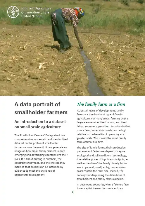
A data portrait of smallholder farmers An introduction to a dataset on small-scale agricultureThe Smallholder Farmers’ Dataportrait is a comprehensive, systematic and standardized data set on the profile of smallholder farmers across the world. It can generate an image on how small family farmers in both emerging and developing countries live their lives. It is about putting in numbers, the constraints they face, and the choices they make so that policies can be informed by evidence to meet the challenge of agricultural development. The family farm as a firmAcross all levels of development, family farms are the dominant type of firm in agriculture. For many crops, farming over a large area requires hired labour, and hired labour requires supervision. For a family that runs a farm, supervision costs can be high relative to the benefits of operating at a greater scale. This makes the small family farm optimal as a firm.The size of family farms, their production patterns and factor use depend on agro-ecological and soil conditions, technology, the relative prices of inputs and outputs, as well as the size of the family. Family farms are, in general, small, as high supervision costs contain the farm size. Indeed, the concepts underpinning the definitions of smallholders and family farms coincide.In developed countries, where farmers facelower capital transaction costs and can1spread capital over large areas, some family farms can be relatively large. In developing countries, families farm small plots of land: they face low transaction costs in labour, engage more workers per hectare, who being family, are motivated to work. This gives them a productivity advantage over larger farms. In some regions, such as Latin America and East Europe, family farms coexist with large corporate farms. Today’s smallho lder farm unwrappedThe success of the Green Revolution in Asia put small family farms, or smallholders, firmly on the development agenda. Productivity growth in smallholder farms contributes towards growth not only by reducing the price of staple food, but also by increasing the demand for labour in rural areas, generating jobs for the poor and raising the unskilled labour wage rate. However, i n today’s modern markets, smallholder farmers must overcome considerable constraints. Sales through sophisticated channels, such as supermarkets, require greater managerial skills and an ability to provide continuity of supply and meet food safety, certification and quality requirements. Agricultural research is becoming increasingly private, focusing on technologies which are knowledge intensive, being developed for larger, commercial farms. This renders technology adoption by small farmers difficult. Smallholder farms face considerable difficulties in accessing credit, as banks are often reluctant to lend due to poor collateral and lack of information. These market failures potentially offset any advantage small farmers may have in productivity. Smallholder farms and development from one region to anotherThe differences in family farms between countries are significant. Equally significant are the differences in the stages of structural transformation across regions. Africa has been bypassed by the Green Revolution and a share of its people experience extreme poverty and hunger. Paradoxically, Africa has been urbanizing fast, but labour productivity in agriculture is low and farm sizes decline. The development agenda highlights the need to stimulate labour productivity in smallholder farms through technical change and promote market participation.Latin America is now urbanized and in many countries smallholder farms coexist with larger commercial farming enterprises. Within the family farm sector, the inequality is pronounced, in spite past land reform policies. Extra efforts may be needed not to bypass or squeeze out smallholder farmers. Some policy prescriptions for growth incline towards increasing smallholder competitiveness, or expanding their asset base through further redistributive interventions. Other measures focus on longer run solutions, and tend to favour enhancing human capital and managing rural poverty through cash transfers.Asia offers many positive lessons on agricultural development but rural poverty remains a problem. In spite of agricultural productivity increases and the fast-growing industrial sector, many Asian countries have undergone a structural transformation characterized by a slow rate of urbanization. Although farmers close to urban centres are becoming increasingly commercial due to strong demand by consumers – who are rapidly diversifying and enriching their diets– more and more smallholder farmers are cut off from modern supply chains. Rural population growth, in conjunction with slow urbanization, also means that policy makers should pay attention to the rural non-farm sector through the creation of a large number of jobs outside agriculture.The need for informationAcross the development policy fora, there is no clear consensus on the likely future direction of small family farm agriculture. Smallholders are the centre of interest by many, but opinions differ on where it is best for them to be in the future. The focus on the importance of structural transformation is weak.This lack of focus is strongly reflected on the availability of information on small-scale agriculture. In spite of the wealth of data, in the form of censuses and household surveys, a comprehensive, systematic and standardized data set on the profile of smallholder farmers across the world has still to be developed. There is need to know, how much and what food is produced by smallholder farmers, how much of their income is generated by farming, how much produce they sell, which is their asset base and much more.Such information will generate an array of benefits: first, it will underline the strengths but also the weaknesses of small-scale family agriculture in many countries, highlighting its linkages with the rural and wider economies and help assess the potential for development; second, it will uncover the main constraints to agricultural development and underscore their importance across countries and regions; third, it will provide valuable insights for the formulation of policy options at national, regional and global levels; and, fourth, it will serve as a platform for advocacy for the role of smallholder farms in growth, emphasizing the fact that their evolution is both the cause and the effect of development.This note introduces a systematic data set for smallholders covering many countries across the world, both developing and emerging. The dataset – being developed in FAO – estimates the number of smallholders and with eight concise indicator groups draws a portrait of smallholder agriculture. In other words, the data ‘take stock’ of smallholder farmers across countries, identify their characteristics in terms of production, technologies, capital assets, access to markets, contribution to rural income, well being, food security and poverty, and, to some extent, highlight the effects of policies and programmes. Who and how manyThere is no unique and unambiguous definition of a smallholder. Often scale, measured in terms of farm size is used to classify farmers. Often, households with less than a threshold land size may be characterized as smallholder. For example, smallholders are often those who farm less than a threshold size of 2 hectares. However, across countries, the distribution of farm sizes depends on a number of agro-ecological and demographic conditions and economic and technological factors.An effort to identify smallholders and vary the threshold size from one country to another, thus taking into consideration agro-climatic conditions was made for a limited number of countries by FAO.1 The Data1FAO (2010). Policies and institutions to support smallholder agriculture. Committee on Agriculture, 22nd Session, 2010.Portrait for Smallholder Farmers does utilize thresholds that take into consideration country-specific factors. The middle-sized farm is one such threshold.2 It is determined by the hectare weighted median and is calculated by ordering farms from smallest to largest and choosing the farm size at the middle hectare as the threshold to choose smallholders and non smallholders in each country.This threshold for smallholder farms and the indicators, are estimated utilizing household surveys, such as the FAO Rural Income Generating Activities database and the Living Standards Measurement Surveys, in combination with agricultural censuses and other information.The Data PortraitThe Smallholder Farmers’Data Portrait has a number of attributes. First, it is being developed t be as ‘global’ as possible. Second, it provides a clear picture of smallholder agriculture, bringing out its strengths and weaknesses: Scale, productivity, technology, commercialization and well-being. Third, it is designed in such a way as to reveal differences between countries and regions in terms of structural transformation; and fourth, it includes policies and programmes to any extent possible.About 30 indicators are adequate to draw a clear portrait of smallholder agriculture. Table 1 shows these indicators, organized in 8 groups, which through the data, depict the main characteristics of smallholders. General indicators, such as the average smallholding size and the number of smallholders, provide an overall idea about farm structure in each 2Key, N. and M. Roberts (2007). Measures of trends in farm size tell differing stories. Amberwaves, November. country. Production indicators take into account food and non food commodities, as well as productivity. Income and pluri-activity indicators show how income is generated on- and off-farm and assess whether smallholder farm households are classified as poor or non poor. They also underscore the importance of farm and non-agricultural activities.Data on labour highlight the importance of family farm as a firm, but also that of the rural economy in supporting livelihoods, by illustrating both the demand and the supply of rural labour. Capital and inputs reflect the base of productive capital of smallholder farms, together with irrigation investments and mechanization. Innovation and technology are covered by data on the use of improved seeds, which reflects the adoption of technology, together with the use of extension services.Access to output and input markets describe the extent of commercialization of small farms. Information on the access to credit also provides a pointer for investment. Transport and communication infrastructure are also portrayed. The inclusion of policies and programmes in the data portrait, when available, can support the assessment of their effectiveness. Demographic indicators also introduce gender and youth dimensions in underpinning both food security, but also investment.Table 1 – Indicators of the smallholder farmers’ data portraitNotes:1.Farm size refers to average land operated by the family for crop production in hectares. Minimum and maximum farm sizes for smallholder and otherfarms are also reported.2.Value of crop production includes all crops produced on the farm. Value of food produced excludes cash crops.3.Household income refers to gross annual earnings from all income generating activities (i.e. on-farm, agricultural wages, off-farm self-employment orwage earning, transfers and other).4.Family labour days on-farm supplied over a day refer to the total number of person-days family members spend on- farm during one working day. Hiredlabour days on-farm and family labour days in off-farm activities are computed similarly.5.All animals are included in the calculation of livestock in Tropical Livestock Units. Depending on the country, these refer to horses, donkeys, oxen, cows,sheep, goats, lambs, pigs, chicken, and ducks.6.% of improved to total seeds is the ratio between quantity of improved seeds to the total quantity of seeds.7.% of expenditure for inputs on value of production refers to the ratio between the total value of inputs to the value of agricultural production.8.The average years of education at school is reported for the head of the household.6。

调查报告英语作文四百字左右Survey Report on Community Health and Well-being.Introduction.This survey report presents the findings of a comprehensive investigation into the health and well-being of our community residents. Conducted through household surveys and focus group discussions, the survey aimed to assess current health status, identify health concerns, and collect data on factors impacting overall well-being.Demographics.The survey sample included residents from various backgrounds, ages, and income levels. The majority of respondents were female (63%), while the age distribution ranged from 18 to 80 years old, with the largest proportion (42%) falling within the 30-49 age group.Health Status.The survey revealed a generally positive self-reported health status, with 65% of respondents rating their health as good or excellent. However, chronic health conditions were also prevalent, with 32% of respondents reporting at least one chronic condition. The most common conditions included hypertension, diabetes, and heart disease.Health Concerns.When asked about their top health concerns, respondents highlighted issues such as mental health (35%), access to healthcare (27%), and unhealthy diet (22%). Mental health concerns included stress, anxiety, and depression, which had increased significantly since the onset of the COVID-19 pandemic. Access to healthcare was cited as a barrier for many, particularly those lacking insurance or facing financial constraints.Factors Impacting Well-being.Beyond physical health, the survey also exploredfactors that influenced residents' overall well-being. Key factors identified included:Social connections: Strong social ties and a sense of community contributed to increased well-being.Physical activity: Regular exercise and physical activity were associated with improved mental and physical health.Purpose and meaning: Having a sense of purpose and engagement in meaningful activities enhanced overall well-being.Economic security: Financial stability and access to basic necessities were essential for maintaining health and well-being.Housing: Safe and stable housing conditions played a vital role in supporting health and well-being.Recommendations.Based on the survey findings, several recommendations were developed to address the identified health concerns and improve community health and well-being:Prioritize mental health support: Expand access to mental health services and provide community-based programs to address rising mental health issues.Improve healthcare access: Implement policies and programs to increase affordable healthcare coverage and reduce financial barriers to care.Promote healthy lifestyles: Encourage healthy eating habits through nutrition education programs and facilitate access to fresh, affordable produce.Nurture social connections: Foster community engagement initiatives and support organizations that create opportunities for socialization and support.Address economic disparities: Implement economic policies and programs that reduce poverty and promote financial stability for all community members.Provide safe housing: Ensure access to affordable and safe housing for all residents, particularly vulnerable populations.Conclusion.The survey report provides valuable insights into the health and well-being of our community residents. By addressing the identified health concerns and implementing the recommended actions, we can create a healthier and more vibrant community where all residents thrive. This report serves as a catalyst for ongoing efforts to improve the health and well-being of our community for generations to come.。

Land rental market,off-farm employment and agricultural production in Southeast China:A plot-level case studyShuyi FENG a,⁎,Nico HEERINK a,b ,Ruerd RUBEN c ,Futian QU aa College of Public Administration,Nanjing Agricultural University,Nanjing 210095,PR Chinab Development Economics Group,Wageningen University,The NetherlandscCentre for International Development Issues,Radboud University,Nijmegen,The Netherlandsa r t i c l e i n f o ab s t r ac tArticle history:Received 4April 2009Received in revised form 31May 2010Accepted 15June 2010This paper performs a plot-level analysis of the impact of land rental market participation and off-farm employment on land investment,input use,and rice yields for 215plots cultivated by 52households in three villages in Northeast Jiangxi Province.Our findings show that households that rent extra land are relatively more productive,but contradict results of earlier studies which found that tenure status of plots affects the level of land investments.We further find that off-farm employment does not signi ficantly affect rice yields.This result contradicts those of earlier studies which found that the negative lost-labor effect of off-farm employment dominates the positive income effect.Another novel finding is that people working locally off-farm tend to switch from green manure planting towards the use of organic manure on their rice plots.We conclude that policies that will further stimulate the development of land rental markets,which is still in its infancy,can contribute signi ficantly to higher rice production in Southeast China.Another implication of our results is that worries about the negative impact that the continuously growing off-farm employment may have on China's goal to remain self-suf ficient in grain production are less relevant at the moment for the region examined in our study.©2010Elsevier Inc.All rights reserved.JEL classi fications:J22Q12Q15Keywords:Land rental market Land tenure contracts Off-farm employment Rural households China1.IntroductionEconomic reforms implemented since the end of the 1970s have stimulated the development of land and labor markets in rural China.Recent studies show an increasing incidence of land rental activities (Deininger &Jin,2005;Kung,2002),while off-farm employment has become a signi ficant phenomenon since the mid-1980s.By 2000,more than 200million rural laborers worked off-farm (de Brauw,Huang,Rozelle,Zhang,&Zhang,2002;Zhang,Huang,&Rozelle,2002).As China's economy continues to grow,the development of land and labor markets is expected to continue or even accelerate.These developments may have important consequences for agricultural production.Land rental markets can enhance allocative ef ficiency and agricultural productivity by equalizing the marginal product of land across households with different land –labor endowments and by facilitating transfers of land from less productive households to more productive ones (Carter &Yao,2002;Deininger,2003;Jin &Deininger,2009).However,in present-day China land rental arrangements are generally informal,short term,and between households living in the same village.Rented plots are therefore subject to tenure insecurity,which may discourage land investment and hamper agricultural productivity increases.The effect of off-farm employment on agricultural production is ambiguous.Off-farm employment reduces the labor available for agricultural production,especially if hiring agricultural labor to replace family labor incurs transaction costs and if hired labor is not as ef ficient as family labor.But off-farm employment also enables households to increase their incomes,to overcome creditChina Economic Review 21(2010)598–606⁎Corresponding author.Tel.:+862584396009;fax:+862584396531.E-mail address:shuyifeng@ (S.Feng).1043-951X/$–see front matter ©2010Elsevier Inc.All rights reserved.doi:10.1016/j.chieco.2010.06.002Contents lists available at ScienceDirectChina Economic Reviewand insurance constraints and to increase their investment in agricultural production (Rozelle,Taylor,&de Brauw,1999;Taylor,Rozelle,&de Brauw,2003).In addition,the reduction in food consumption by household members working off-farm (e.g.those who migrate)may have an impact on agricultural production decisions if household production and consumption decisions are non-separable (Burger,1994).Few studies provide empirical estimates of the effect of land rental market development on allocative ef ficiency and agricultural productivity in rural China.Carter and Yao (2002)find for a panel data set of 339households,surveyed in 1988,1993and 1997in five counties in Zhejiang and Jiangxi Provinces,that allocative ef ficiency is achieved by households that rent out land,but surprisingly not by households that rent in land.Lohmar,Zhang,and Somwaru (2001)find for a sample of 830households,surveyed in 1998in 6provinces,that allocative ef ficiency and aggregate agricultural production increase,because the households that rent in land have a signi ficantly higher marginal product of land than households that do not rent additional land.Jin and Deininger (2009)examine the impact of land rentals using a panel of almost 8,000households in about 800villages that are representative of China's nine agriculturally most important provinces for the period 2001–2004.Their study finds that,by transferring land from less able and more af fluent households who joined the non-farm sector to poorer ones with ample family labor,land markets allow more effective use of potentially idle land that can contribute to signi ficant agricultural productivity gains.Related research on land tenure in rural China focuses on the land tenure insecurity resulting from frequent land reallocations,and the impact of this insecurity on household investment (as measured by application of green manure or organic manure)and agricultural productivity (Benjamin &Brandt,2002;Jacoby,Li,&Rozelle,2002;Li,Rozelle,&Brandt,1998).Rural land in China belongs to the village collectives,with farm households having user rights for a fixed contract period (at the moment 30years for most cultivated land).Land is generally allocated to farm households on the basis of their household (and/or labor force)size,but may be reallocated to correct for demographic changes (Tan,Heerink,&Qu,2006).Most studies investigating the insecurity caused by reallocations find that it has a signi ficant but small negative effect on investment (e.g.green manure,organic manure),but no signi ficant effect on productivity.The main explanation is that land investment plays a minor role in agricultural production compared with other agricultural inputs such as land,labor,and chemical fertilizers (Yao,2007).Many empirical studies have investigated the effect of off-farm employment on agricultural production in rural China.Recent studies in this field apply the “new economics of labor migration ”(NELM)framework developed by Stark and Bloom (1985),in which the migration decision is part of a set of interwoven economic choices made by households facing imperfect markets.Rozelle et al.(1999)and Taylor et al.(2003)estimate a simultaneous-equation model from data collected among 787farm households from 31villages in Hebei and Liaoning Provinces in 1995,and find the positive income effect of migrant remittances nearly offsets the negative lost-labor effect of migration on crop production.On the other hand,using a village computable general equilibrium model that takes into account existing factor market imperfections,Shi et al.(in press)find for a remote village in Jiangxi Province that the negative lost-labor effect of off-farm employment on agricultural incomes is much stronger than the (small)positive income effect.None of these studies,however,pays attention to the reduced food consumption effect identi fied by Burger (1994).To our knowledge no studies have analyzed until now the joint impact of land rental market development and off-farm employment on agricultural production in China.Rural China is characterized by surplus and underemployed rural labor,while land rental markets are rather thin (Brandt,Huang,Li,&Rozelle,2002;Brandt,Rozelle,&Turner,2004).Rural households facing such land and labor market imperfections are likely not to make decisions on land and labor market participation in isolation,but to decide on them simultaneously.The purpose of this paper is therefore to analyze the joint effects of land rental market participation and off-farm employment on agricultural production in rural China.We will investigate the impact on land investment,input use,and agricultural productivity separately,as the land renting and off-farm employment may affect each aspect differently.The remainder of this paper is structured as follows.Section 2presents the theoretical framework of our analysis.Section 3introduces the estimation procedure.In Section 4,estimation results are presented.The paper concludes with a summary of its main findings and with some policy implications in Section 5.2.Conceptual frameworkIn this paper we will use plot-level data to examine the impacts of land renting and off-farm employment on agricultural production.The model employed is based on the structural models developed by Feder,Onchan,Chalamwong,and Hongladarom (1988),Place and Hazell (1993)and Hayes,Roth,and Zepeda (1997)to examine the impact of tenure security on investments,input use and productivity in agriculture.Assuming that households decide on land renting and off-farm employment before making decisions on land management and investment 1,the reduced-form equations can be written as follows:LI i =LI i A in ;l o ;TS i ;Z p i ;Z q ;Z h;L ;A ;r ;w ;p X ð1Þl a i =l a i A in ;l o ;TS i ;Z p i ;Z q ;Z h;L ;A ;r ;w ;p X ð2ÞX i =X i A in ;l o ;TS i ;Z p i ;Z q ;Z h;L ;A ;r ;w ;p X ð3ÞQ i =Q i A in ;l o ;TS i ;Z p i ;Z q ;Z h;L ;A ;r ;w ;p Xð4Þ1This assumption will (partly)be relaxed in our empirical analysis.599S.Feng et al./China Economic Review 21(2010)598–606600S.Feng et al./China Economic Review21(2010)598–606where LI,l a,X,and Q are land investment,labor use,use of non-labor inputs,and yield on each plot(subscript i),respectively.The explanatory variables A in and l o are household decisions on whether to rent additional land and participate in off-farm employment,respectively.TS is the plot-specific tenure security indicator,Z p are other plot characteristics,Z q are farm characteristics,Z h are household preferences,L is the household labor endowment,A is the land endowment,r is the market land rent,w is the market labor wage,and p X is the price for non-labor inputs.By estimating Eqs.(1)–(4),the total(i.e.direct plus indirect)effects of land renting(A in),the resulting tenure security of plots(TS),and off-farm employment(l o)on land investment, labor use,non-labor inputs,and land productivity can be assessed.3.Model specification and estimationThis paper uses data from a farm household survey and a plot-level survey that were held in three villages in Northeast Jiangxi Province,Southeast China.The villages were selected using a series of criteria including economic development level,market access and geographical conditions.Local researchers and policy makers were consulted and several site visits were made as part of this process.The three villages are considered representative of the diversity of rural conditions that can be found in Northeast Jiangxi Province and in the much larger hilly area of Southeast China with rice-based production systems(Kuiper,Heerink,Tan,Ren,&Shi, 2001).The three villages selected are Banqiao in Yujiang County,Shangzhu in Guixi City and Gangyan in Yanshan County2.The farm household survey was carried out in2000and the beginning of2001.The questions in the survey referred to the entire year2000.In each village,23%of the households were interviewed.A stratified random sample was used for selecting the households,with the hamlets within each village forming the strata(Kuiper et al.,2001).The information collected includes demographic characteristics,assets,land tenure,and participation in factor markets.Data on household migration and local off-farm employment decisions collected during that survey are used for the empirical analysis below.Plot-level data,however,were not collected then.Out of the329households interviewed in2000and2001,52households were randomly selected,and plot-level agricultural production data were collected in January2003for the entire year2002.Of the52 households in the three villages,19households rented in irrigated land in2002,while33households did not(and are therefore considered ‘self-sufficient in land’).Plots cultivated with rice,the most important crop in the research area,are included in the sample.In total215rice plots were surveyed;172were contracted directly from village collectives and43(i.e.20%of the plots)were rented from other farm households.Contracted plots occur in both self-sufficient households and households that rent in,while rented plots are restricted only to households that rent in.Collected information includes input use and output of each plot,plot characteristics,and soil quality.3.1.Model specificationThe conceptual framework in Section2suggests the variables that potentially affect agricultural production decisions.An overview of the dependent and explanatory variables included in the analysis,subdivided by household land market regimes(land renting in vs.self-sufficient in land)and tenure status of the plot(contracted vs.rented),is presented in Table1.Land investment is represented by green manure planting(LI gm)and organic manure application(LI om)3;long-term land investments,such as wells,fences or fruit trees,are virtually absent on the rice plots examined in our study.The land investment variables are both dummy variables which equal one if the household invests on the plot.As can be seen from Table1,green manure is planted on33%of the plots,and organic manure is applied on46%of the plots in the sample.Input use includes labor(l a)and chemical fertilizers(X cf)4.These inputs are expressed per unit area to correct for differences in plot bor is measured in man days.There arefive different commonly used types of chemical fertilizers,which are aggregated and measured in value terms.Households work on average around41days and use47yuan of chemical fertilizers on each mu of land(see Table1).Households grow either a single or a double rice crop in the surveyed area.Rice yields(Q)vary for different varieties and are aggregated and measured in values per unit area.As can be seen from Table1,the average rice yield is297.73yuan per mu5.Explanatory variables in the analysis include household decisions in terms of land renting in(A in)and off-farm employment (l o),indicators of plot tenure security(TS),plot characteristics(Z p),farm characteristics(Z q),household characteristics(Z h), household land and labor endowments(A and L),market land rent(r),market wage rate(w),and non-labor input prices(p X).Households that rent land(A in)are expected to have a higher marginal product of land,and therefore a higher agricultural productivity,than those that do not.The impact of off-farm employment(l o)on agricultural investment,input use and production is ambiguous,as explained in Section1.If the income effect dominates the sum of the lost-labor and reduced food consumption effects,the net impact will be positive;if the latter two effects are stronger,it will be negative.In our analysis we distinguish between local off-farm employment(l ol)and migration(l om)6.Local off-farm employment may only have an income effect,2See Feng and Heerink(2008)for a detailed introduction of the three villages.3The research on the effect of tenure security on land investment focuses on the use of green manure planting and organic manure application as the main forms of land investment in rural China(Jacoby et al.,2002;Li et al.,1998).4Data are also available on seed,herbicides and pesticides and animal traction.These inputs are not included in the analysis for simplicity,because they are relatively minor inputs.5The calculation of the rice yield is based on prices for the year2002.Since the autumn of2003,rice prices have increased rapidly.6Migrants are family members working off-farm and not living together with other household members.Households participate in migration if at least one household member works as a migrant.They participate in local off-farm employment if they have at least one household member working off-farm but no household members working as migrants.because household members that are involved in local off-farm employment normally live and consume at home and are often able to combine local off-farm employment with on-farm agricultural production.For migration,on the other hand,all three effects may be relevant.Tenure security (TS )is represented by the tenure status of the plot.Plots are either contracted from the village collectives (for a 30-year period)or rented from other households.A dummy variable,which equals one if the plot is rented,is used to indicate the tenure status.The land rental arrangements are normally verbal and of short duration.Rented plots are therefore less secure than contracted plots and are expected to receive less land investment,and thus to produce less output.On the other hand,the use of variable inputs is expected to be higher on rented plots because households renting additional land tend to maximize short-term agricultural pro fits on these plots.Thus the net effect of tenure security on yield is ambiguous.Following Pender and Fafchamps (2001),the interaction between the household land renting variable and the rented plot dummy (A in *TS )is included in the model.In this way it is possible to examine whether rented plots are managed in a signi ficantly different way compared to non-rented plots,given that households that rent additional land may have a higher productivity than ‘self-suf ficient ’households.The control variables in model (1)–(4)consist of plot characteristics (Z p ),farm characteristics (Z q ),household characteristics (Z h ),household time and land endowments (L ,A )and market land rent,wage rate and non-labor input prices (r ,w ,p X ).Plot characteristics comprise the following indicators:-Soil fertility (Z pf ).Households in the survey were asked their perceptions about soil quality,which were given a value of one if households perceived soil fertility as poor,two if households perceived soil fertility as average,and three if households perceived soil fertility as good.It is expected that land productivity is higher on plots with good soil nd investment and input use may be higher on fertile plots,if the marginal returns of land investment and input use are higher than on plots with poor soil fertility.They are expected to be lower,if the marginal returns are lower.Table 1Descriptive statistics of the variables used in the plot-level analysis.Source:Farm household survey.ItemSymbolsUnitRenting in household (19)Self-suf ficient household (33)All plotsContractedRentedContracted Number of sample plots6043112215Mean (standard deviation)Dependent variables Land investment Green manure LI gm 0or 10.32(0.47)0.19(0.39)0.39(0.49)0.33(0.47)Organic manure LI om 0or 10.50(0.50)0.37(0.49)0.47(0.50)0.46(0.50)Input use Laborl a Man day/mu b 37.6(20.0)37.7(36.0)43.4(19.6)40.6(23.9)Chemical fertilizers X cf Yuan c /mu 54.0(30.9)54.9(13.5)40.3(21.7)47.0(24.4)Rice yieldQYuan /mu327(79.8)355(81.4)260(79.1)298(89.3)Independent variablesHousehold factor allocation Renting land aA in0.72(0.26)0.76(0.24)0.14(0.20)0.43(0.37)Renting land a ×rented plot interaction A in *TS 0.00(0.00)d0.76(0.24)d0.00(0.00)0.15(0.32)Participating in migrationl om 0or 10.53(0.50)0.40(0.49)0.54(0.50)0.51(0.50)Participating in local off-farm employment l ol 0or 10.20(0.40)0.12(0.32)0.29(0.45)0.23(0.42)Plot characteristics Rented plot TS 0or 10.00(0.00) 1.00(0.00)0.00(0.00)0.20(0.40)FertilityZ pf 1.93(0.84) 2.09(0.84) 1.93(0.80) 1.96(0.82)Topsoil depth Z ptd cm 16.7(4.54)17.8(3.86)16.4(3.74)16.8(4.02)Plot sizeZ pps Mu 1.83(1.17) 2.46(2.59) 1.49(1.23) 1.78(1.62)Distance from home Z pd Minute11.8(8.22)d 17.9(13.6)d11.2(10.3)12.7(10.8)Farm characteristicsTotal number of cattle Z qc 1.17(1.76) 2.16(3.22)0.67(0.47) 1.11(1.82)Age of household headZ qa Years 51.2(13.1)46.8(13.3)45.5(9.81)47.3(11.7)Education of household head Z qe Years3.78(2.49)4.37(2.61)5.24(2.86) 4.66(2.78)Female to male adult ratio Z qfm 1.12(0.67) 1.14(0.57) 1.09(0.69) 1.11(0.66)Number of plotsZ qp 4.33(1.74)4.30(1.32)4.98(1.96)4.67(1.81)Household characteristics Household sizeZ hhs Persons 5.60(1.44) 5.40(1.43) 4.79(1.91) 5.13(1.73)Number of dependents Z hd Persons1.98(1.32)2.26(1.42) 1.39(1.02) 1.73(1.24)Number of durable assetsZ hda 7.08(1.41)7.30(1.32) 6.46(1.67) 6.80(1.57)Household land and labor endowment Irrigated land per adult IA Mu 2.39(1.65)d3.25(2.10)d2.06(1.38) 2.39(1.68)Village dummies Banqiao Dummy BQ 0or 10.22(0.42)0.12(0.32)0.34(0.48)0.26(0.44)Shangzhu DummySZ0or 10.15(0.36)0.07(0.26)0.55(0.50)0.34(0.48)Note:a :Household renting in decisions are predicted probabilities derived from a probit model.b :1mu=1/15ha.c :1USD =6.83yuan (exchange rate on October 27,2009).d :Difference in means within renting in household group is statistically signi ficant for results highlighted in bold.601S.Feng et al./China Economic Review 21(2010)598–606-Topsoil depth (Z ptd )is estimated by soil scientists,and measured in centimeters.The expected impact on yields,land investments and input use are similar to those for soil fertility.-Plot size (Z pps ).Large plots are easier to manage and have higher input use ef ficiency (economies of scale).They are therefore expected to receive fewer inputs,have higher yields,or both.-Distance from home (Z pd ).The distance between the homestead and each plot is measured in minutes travel time.Longer travel time raises the cost of carrying organic manure and other inputs to the plots.Planting green manure on distant plots is sometimes risky because of high supervision costs involved in keeping out wild animals.A larger distance from home is thus expected to reduce land investment,input use and rice yield.The square of this variable is added to the equation to capture possible nonlinearities in its impact.Farm characteristics included in the model comprise:-Number of cattle (Z qc ).Cattle are very important draft animals for small-scale households in rural China.Their use is expected to have a positive impact on land productivity.Moreover,organic manure cannot be exchanged in the market in the research area.Therefore a larger number of cattle in a household are expected to increase land investment,and thereby also raise land productivity.-Age of the household head (Z qa ).Older farmers have more experience and are therefore expected to be more productive in agriculture.In addition,older farmers like to stick to farming traditions,so green manure planting and organic manure application may be higher while chemical fertilizer application may be lower.-Education of the household head (Z qe ).Household heads with more schooling (in years)are expected to have more farming skills and therefore to be more productive in agriculture.Well-educated farmers may also be more aware of the potential bene fits of land investment.-Female to male adult ratio (Z qfm )is used to test for differences between females and males in physical strength or other factors in fluencing agricultural production.Transporting organic manure and cutting the roots of green manure for land preparation requires much physical strength.It is therefore expected that a higher female –male adult ratio leads to less land investment and more chemical fertilizer use.-Number of plots of the household (Z qp )is an indicator of land fragmentation.It can have either negative or positive effects on agricultural production (Tan,Heerink,Kruseman,&Qu,2008).On the one hand,a larger number of plots need more labor to manage (Nguyen,Chen,&Findlay,1996).On the other hand,it enables the households to diversify agricultural production and reduce risk (Bentley,1987),and to optimize their labor allocation over different crop varieties and seasons,especially when there is no market for agricultural labor (Fenoaltea,1976).Household characteristics have a direct effect on household consumption preferences,and can have either positive or negative effects on the demand for leisure and consumption goods.If household decisions are non-separable,this will affect production decisions as well.The household characteristics included in our model are:-Household size (Z hhs ).A larger household needs more food than a small one,so the household size is expected to have a positive impact on land investments,input use and rice yields.-Number of dependents in a household (Z hd ).A household with more dependents needs less food than a household with many adults.So,the impact of this variable is expected to be opposite to that of household size.-Female to male adult ratio (Z qfm )does not only have a direct impact on production decisions (see above),but is also likely to affect consumption decisions,because female adults tend to consume less food than male adults.Hence,the impact of this ratio is expected to be similar to that of the number of dependents.-Number of durable assets in a household (Z hda ).Wealthier households tend to consume more food,hence the number of durable assets is expected to have a positive impact on land investments,input use and rice yields.The household time endowment equals household size (Z hhs )minus the number of dependents (Z hd ).In addition,household time endowment may depend on the ratio of female to male adults (Z qfm ),as taking care of children and doing housework is usually a female task in Chinese society.If household decisions are non-separable,land investment,labor use,and rice yield are expected to be positively related to the household labor endowment.The household land endowment is represented by the total size of contracted irrigated land per adult (IA ).If household decisions are non-separable,land investment,labor use and rice yield are expected to be negatively related to the household land endowment.The market land rent (r ),wage rate (w ),and non-labor input prices (p X )are assumed to be the same for all households living in the same village.They are therefore captured by village dummy variables for Banqiao (BQ )and Shangzhu (SZ ).The resulting model that is used for estimation can be speci fied as follows:DV i =α0+α1A in+α2A in*TS i +α3lom+α4lol+α5ln Z pf i +α6ln Z ptd i +α7ln Z pps i ÀÁ+α8ln Z pd i +α9ln Z pdi 2+α10ln Zqc ÀÁ+α11ln Z qa ÀÁ+α12ln Z qe ÀÁ+α13ln Zqfm+α14ln Z qp ÀÁ602S.Feng et al./China Economic Review 21(2010)598–606+α15ln Zhhs +α16ln Z hd +α17ln Z hda +α18ln Z IA+α19BQ +α20SZ +v ið5Þ–ð9Þwith:DV i =LI gmi (green manure planting),LI omi (organic manure application),X cfi (chemical fertilizer use),l ai (labor use),and Q i(rice yield per mu ),respectively;α0,...,α20are unknown coef ficients,v i is a disturbance term with standard properties,and i =1, (215)3.2.Estimation methodThe estimation of Eqs.(5)–(9)is based on the nature of each dependent variable.The land investment variable is binary,and thus estimated by a probit model.Input use and rice yield variables are continuous,and thus estimated by ordinary least squares regression.All explanatory variables in the analysis are exogenous,except for households'decisions of land renting in (A in ),migration (l om )and local off-farm employment (l ol ),which may be endogenous as they depend on household characteristics,farm characteristics,household land and labor endowments,institutional factors,and market rent,wage,and other prices.As mentioned,data on household migration and local off-farm employment decisions was collected for the year 2000,while data on plot-level agricultural production was collected for the year 2002.Households'decisions of migration and local off-farm employment were therefore taken before the agricultural production decisions and are treated as exogenous in our analysis.Decisions on renting extra land were made in the year 2002and may therefore be endogenous.Inclusion of endogenous variables in the estimation may result in biased estimates.Instrumental variables are used to address this problem.First,a probit model is used to estimate land renting at the farm household level 7.Next,the resulting predicted probabilities of households renting additional land are used as an instrument for the households land renting variable (A in )in the estimation of Eqs.(5)–(9).Estimated standard errors are robust to heteroskedasticity and possible non-independence of different plots managed by the same household for all five regressions.4.Regression resultsTable 2shows the estimation results for each of the five dependent variables.A first noteworthy finding is that households renting additional land have higher rice yields per mu ,but their land investment and input levels do not differ signi ficantly from those of other households.Hence,their productivity per unit of land,labor and chemical fertilizer is higher.We further find that households that rent extra land use signi ficantly more chemical fertilizer on the rented plots,as compared to their contracted plots,as is evident from the result for the interaction variable.Levels of soil fertility,however,do not differ signi ficantly between rented and contracted plots (see Table 1).A possible explanation for the higher use of chemical fertilizers may be that farmers are less familiar with the plots that they rent than the farmers that contract that plot and therefore tend to over-apply chemical fertilizers on such plots.Yield levels are not signi ficantly affected,as is evident from the insigni ficant coef ficient estimate for the interaction variable in the yield nd investments also do not differ signi ficantly between rented and contracted plots.The latter finding contradicts earlier results by Jacoby et al.(2002)and Li et al.(1998)that tenure security has a positive effect on land investment.Their studies focus on land reallocations as a source of tenure insecurity,whereas our study examines the impact of (usually oral)land rental contracts.The fact that land renting almost exclusively takes place between households,often relatives,living in the same village may explain why households use similar quantities of organic and green manure on rented plots as they do on their own contracted plots.With respect to off-farm employment,we find that migration does not affect any of the dependent variables in our analyses,whereas local off-farm employment leads to signi ficantly less green manure planting and signi ficantly higher use of organic manure.The finding that rice yields are not affected by either type of off-farm employment suggests that the income effect is strong enough to counterbalance the negative impact of lost-labor and reduced home food consumption on rice production for the three villages in our sample.The switch from green manure towards organic manure that we observe for households involved in local off-farm employment may have to do with the fact that green manure requires labor input in the slack season,and therefore is less compatible with local off-farm activities.A few interesting results also emerge for the control variables that we use in the regressions.With regard to plot characteristics,we find that better quality plots (in terms of soil fertility and soil depth)receive less land investment,indicating that the marginal return of land investment is higher on plots with poor soil fertility.Levels of input use are not signi ficantly different,but rice yields are signi ficantly higher for plots with better soil quality.Plot size is negative related to green manure planting and labor use,while rice yields are not signi ficantly affected.This finding provides evidence of economies of scale in rice growing.The distance between a plot and the homestead has a signi ficant effect on green manure planting and on labor use 8.An inverted U-shaped relationship is found in both regressions,with the turning points located at a travel time of around 15and 9,respectively.Even though there is less land investment and labor use on far-away plots,rice yields surprisingly are not signi ficantly lower on such plots.7The probit model results can be obtained from the authors upon request.8Data on labor use in the survey include travel time to the plots.The result for labor use should be interpreted with caution.603S.Feng et al./China Economic Review 21(2010)598–606。

不同国家对家庭收入数据统计英语作文Household income data is an important economic indicator that provides insights into the financial well-being of a country's population. However, the methods used by different nations to collect and report this information can vary significantly. This essay will explore the approaches taken by several major economies in gathering and publishing household income statistics.In the United States, the primary source of household income data is the Current Population Survey (CPS), conducted monthly by the U.S. Census Bureau. The CPS collects information on the income of households, defined as all the people who occupy a housing unit. Respondents are asked to report their total pre-tax cash income from various sources, including wages, salaries, tips, net self-employment income, interest, dividends, Social Security payments, and other government transfers. The Census Bureau then aggregates this data to calculate measures such as median household income and the income distribution.One notable aspect of the U.S. approach is the exclusion of certainnon-cash benefits, such as employer-provided health insurance, food stamps, and housing subsidies, from the household income calculation. This has been a source of criticism, as these types of assistance can significantly impact a family's financial situation. Additionally, the CPS relies on self-reported data, which may be subject to recall bias or intentional underreporting of income.In contrast, the United Kingdom takes a more comprehensive approach to measuring household income. The Office for National Statistics (ONS) conducts the Family Resources Survey (FRS), which collects data on the income of all individuals within a household, including income from employment, self-employment, investments, and state benefits. The FRS also gathers information on the receipt of various non-cash benefits, such as free school meals and subsidized housing. This allows the ONS to calculate a more holistic measure of household disposable income, which is then used to analyze income inequality and poverty rates.One potential limitation of the UK's approach is the reliance on survey data, which may not capture the full extent of the population's income, particularly for high-income households that may be less inclined to participate in the survey. To address this, the ONS supplements the FRS with administrative data from tax records and other sources to provide a more accurate picture of the income distribution.In Germany, the primary source of household income data is the Socio-Economic Panel (SOEP), a longitudinal survey conducted by the German Institute for Economic Research (DIW Berlin). The SOEP collects detailed information on the income, assets, and living conditions of households, including income from employment, self-employment, government transfers, and private sources. Unlike the U.S. and UK approaches, the SOEP also gathers data on the wealth and financial assets of households, providing a more comprehensive view of their economic well-being.One advantage of the SOEP is its longitudinal design, which allows researchers to track changes in household income and wealth over time. This can provide valuable insights into the dynamics of income mobility and the factors that influence household financial stability. However, the SOEP's reliance on self-reported data may still be subject to some biases, and the sample size, while substantial, may not fully represent the diversity of the German population.In China, the collection and reporting of household income data is a more centralized and government-driven process. The National Bureau of Statistics of China (NBS) conducts the annual Urban Household Survey and the Rural Household Survey to gather information on the income and expenditures of urban and rural households, respectively. These surveys collect data on a range ofincome sources, including wages, salaries, self-employment income, and government transfers.One notable aspect of the Chinese approach is the emphasis on capturing the income of both urban and rural households, reflecting the country's significant rural-urban divide. However, the reliability of the data collected by the NBS has been the subject of some debate, with concerns raised about potential underreporting of income, particularly in the context of China's rapidly changing economic landscape.In Japan, the Ministry of Internal Affairs and Communications (MIC) conducts the Comprehensive Survey of Living Conditions (CSLC) to gather data on household income and expenditures. The CSLC collects information on the income sources of household members, including wages, salaries, pensions, and social security benefits. The data is then used to calculate measures such as average household income and the income distribution.One unique feature of the Japanese approach is the inclusion of in-kind benefits, such as employer-provided housing and meals, in the calculation of household income. This helps to provide a more accurate representation of the overall economic well-being of Japanese households. However, the CSLC, like many other household income surveys, relies on self-reported data, which may be subject tosome limitations.In conclusion, the methods used by different countries to collect and report household income data vary significantly, reflecting the diverse economic and social contexts of these nations. While some approaches, such as those of the UK and Germany, aim to capture a more comprehensive view of household financial well-being, others, like the U.S. and China, may have more limited scopes or face challenges in ensuring the reliability of the data collected.Nonetheless, the availability of household income statistics remains crucial for policymakers, researchers, and the public to understand the economic conditions of a country's population and inform decision-making processes. As economic and social dynamics continue to evolve, it is essential for national statistical agencies to adapt their data collection and reporting methods to ensure that household income data remains a reliable and relevant tool for informed policy discussions and economic analyses.。

县住户调查样本轮换工作总结英文版County Household Survey Sample Rotation Work Summary Introduction:The County Household Survey Sample Rotation is an essential process aimed at ensuring the representativeness, accuracy, and timeliness of data collected from households. This summary outlines the key steps, challenges, and achievements from the recent sample rotation exercise.Sample Rotation Importance:Sample rotation is a vital aspect of maintaining the integrity of household surveys. It ensures that survey respondents are rotated periodically, preventing fatigue and bias. This rotation also allows for the inclusion of new households, reflecting changes in the population and ensuring the representativeness of the data.Process Overview:Planning Phase: The planning phase involved identifying the target population, determining the sample size, and designing the rotation schedule. This phase was crucial as it set the foundation for the entire rotation process.Sample Selection: Samples were selected randomly from the target population, ensuring representativeness across all strata. Strict sampling criteria were followed to minimize biases.Data Collection: Once the samples were selected, data collection began. This involved conducting interviews, surveys, and collecting relevant information from the households.Data Analysis: Collected data was then analyzed to identify trends, patterns, and any potential biases. This analysis helped in refining the survey methods and improving data quality.Feedback and Improvement: Feedback from respondents and stakeholders was collected to identify areas for improvement. This feedback loop ensures continuous quality improvement in the survey process.Challenges Encountered:During the sample rotation, several challenges were encountered, including respondent fatigue, non-response bias, and data entry errors. To address these challenges, regular training sessions were conducted for surveyors, and follow-up interviews were arranged for non-respondents.Achievements:Despite the challenges, significant achievements were made. The sample rotation exercise successfully included new households, improving the representativeness of the data. Additionally, the feedback loop helped identify areas for improvement, leading to more efficient and accurate data collection in future surveys.Conclusion:The County Household Survey Sample Rotation exercise was a comprehensive and successful undertaking. It not only improved the quality and representativeness of the survey data but also established a robust feedback mechanism for continuous improvement. With these achievements, the Countyis well-positioned to conduct future surveys with greater accuracy and efficiency.县住户调查样本轮换工作总结介绍：县住户调查样本轮换是一项重要的工作，旨在确保收集到的住户数据的代表性、准确性和时效性。

家庭节能调研英语作文Title: Research on Household Energy Conservation。

Introduction:In recent years, the issue of energy conservation has become increasingly important due to environmental concerns and the need to reduce household expenses. This research aims to investigate the attitudes, behaviors, and perceptions of households towards energy conservation.Methodology:To conduct this research, a survey was distributed to households in various communities. The survey included questions about energy usage habits, awareness of energy-saving techniques, willingness to adopt energy-efficient technologies, and factors influencing energy conservation behaviors.Findings:1. Awareness and Knowledge:The majority of respondents demonstrated a basic understanding of energy conservation but lacked detailed knowledge about specific techniques and technologies.Many households were unaware of the potential cost savings associated with energy conservation measures.2. Energy Usage Habits:Most households reported using energy-intensive appliances such as air conditioners, heaters, and refrigerators on a daily basis.There was a notable reliance on traditional incandescent light bulbs, despite the availability of more energy-efficient alternatives.3. Attitudes towards Energy Conservation:The majority of respondents expressed a positive attitude towards energy conservation, citing environmental concerns and the desire to reduce utility bills as motivating factors.However, some households expressed skepticism about the effectiveness of energy-saving measures and were reluctant to change their habits.4. Barriers to Energy Conservation:Lack of awareness about energy-saving technologies and their benefits was identified as a significant barrier.Initial cost barriers were also cited, particularly in relation to the purchase of energy-efficient appliances and lighting.5. Potential Solutions:Education and awareness campaigns to promote energyconservation and highlight the benefits of energy-efficient technologies.Financial incentives and subsidies to encourage households to invest in energy-saving measures.Collaboration with utility companies to provide information and support for energy conservation initiatives.Conclusion:Overall, the research findings suggest that while there is a general willingness to engage in energy conservation, there are significant barriers that need to be addressed.By raising awareness, providing education, and offering financial incentives, households can be encouraged to adopt more energy-efficient practices, ultimately leading to both environmental and economic benefits.。