Review of three dimensional holographic imaging by multipleviewpoint projection based methods

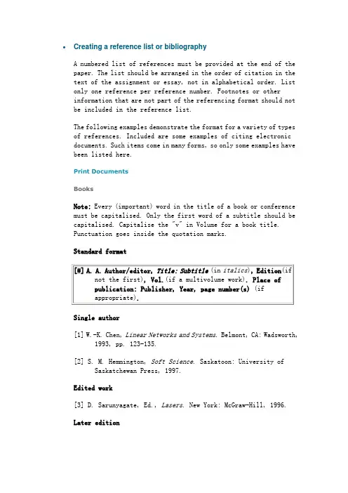
•Creating a reference list or bibliographyA numbered list of references must be provided at the end of thepaper. The list should be arranged in the order of citation in the text of the assignment or essay, not in alphabetical order. List only one reference per reference number. Footnotes or otherinformation that are not part of the referencing format should not be included in the reference list.The following examples demonstrate the format for a variety of types of references. Included are some examples of citing electronic documents. Such items come in many forms, so only some examples have been listed here.Print DocumentsBooksNote: Every (important) word in the title of a book or conference must be capitalised. Only the first word of a subtitle should be capitalised. Capitalise the "v" in Volume for a book title.Punctuation goes inside the quotation marks.Standard formatSingle author[1] W.-K. Chen, Linear Networks and Systems. Belmont, CA: Wadsworth,1993, pp. 123-135.[2] S. M. Hemmington, Soft Science. Saskatoon: University ofSaskatchewan Press, 1997.Edited work[3] D. Sarunyagate, Ed., Lasers. New York: McGraw-Hill, 1996.Later edition[4] K. Schwalbe, Information Technology Project Management, 3rd ed.Boston: Course Technology, 2004.[5] M. N. DeMers, Fundamentals of Geographic Information Systems,3rd ed. New York : John Wiley, 2005.More than one author[6] T. Jordan and P. A. Taylor, Hacktivism and Cyberwars: Rebelswith a cause? London: Routledge, 2004.[7] U. J. Gelinas, Jr., S. G. Sutton, and J. Fedorowicz, Businessprocesses and information technology. Cincinnati:South-Western/Thomson Learning, 2004.Three or more authorsNote: The names of all authors should be given in the references unless the number of authors is greater than six. If there are more than six authors, you may use et al. after the name of the first author.[8] R. Hayes, G. Pisano, D. Upton, and S. Wheelwright, Operations,Strategy, and Technology: Pursuing the competitive edge.Hoboken, NJ : Wiley, 2005.Series[9] M. Bell, et al., Universities Online: A survey of onlineeducation and services in Australia, Occasional Paper Series 02-A. Canberra: Department of Education, Science andTraining, 2002.Corporate author (ie: a company or organisation)[10] World Bank, Information and Communication Technologies: AWorld Bank group strategy. Washington, DC : World Bank, 2002.Conference (complete conference proceedings)[11] T. J. van Weert and R. K. Munro, Eds., Informatics and theDigital Society: Social, ethical and cognitive issues: IFIP TC3/WG3.1&3.2 Open Conference on Social, Ethical andCognitive Issues of Informatics and ICT, July 22-26, 2002, Dortmund, Germany. Boston: Kluwer Academic, 2003.Government publication[12] Australia. Attorney-Generals Department. Digital AgendaReview, 4 Vols. Canberra: Attorney- General's Department,2003.Manual[13] Bell Telephone Laboratories Technical Staff, TransmissionSystem for Communications, Bell Telephone Laboratories,1995.Catalogue[14] Catalog No. MWM-1, Microwave Components, M. W. Microwave Corp.,Brooklyn, NY.Application notes[15] Hewlett-Packard, Appl. Note 935, pp. 25-29.Note:Titles of unpublished works are not italicised or capitalised. Capitalise only the first word of a paper or thesis.Technical report[16] K. E. Elliott and C.M. Greene, "A local adaptive protocol,"Argonne National Laboratory, Argonne, France, Tech. Rep.916-1010-BB, 1997.Patent / Standard[17] K. Kimura and A. Lipeles, "Fuzzy controller component, " U.S. Patent 14,860,040, December 14, 1996.Papers presented at conferences (unpublished)[18] H. A. Nimr, "Defuzzification of the outputs of fuzzycontrollers," presented at 5th International Conference onFuzzy Systems, Cairo, Egypt, 1996.Thesis or dissertation[19] H. Zhang, "Delay-insensitive networks," M.S. thesis,University of Waterloo, Waterloo, ON, Canada, 1997.[20] M. W. Dixon, "Application of neural networks to solve therouting problem in communication networks," Ph.D.dissertation, Murdoch University, Murdoch, WA, Australia, 1999.Parts of a BookNote: These examples are for chapters or parts of edited works in which the chapters or parts have individual title and author/s, but are included in collections or textbooks edited by others. If the editors of a work are also the authors of all of the included chapters then it should be cited as a whole book using the examples given above (Books).Capitalise only the first word of a paper or book chapter.Single chapter from an edited work[1] A. Rezi and M. Allam, "Techniques in array processing by meansof transformations, " in Control and Dynamic Systems, Vol.69, Multidemsional Systems, C. T. Leondes, Ed. San Diego: Academic Press, 1995, pp. 133-180.[2] G. O. Young, "Synthetic structure of industrial plastics," inPlastics, 2nd ed., vol. 3, J. Peters, Ed. New York:McGraw-Hill, 1964, pp. 15-64.Conference or seminar paper (one paper from a published conference proceedings)[3] N. Osifchin and G. Vau, "Power considerations for themodernization of telecommunications in Central and Eastern European and former Soviet Union (CEE/FSU) countries," in Second International Telecommunications Energy SpecialConference, 1997, pp. 9-16.[4] S. Al Kuran, "The prospects for GaAs MESFET technology in dc-acvoltage conversion," in Proceedings of the Fourth AnnualPortable Design Conference, 1997, pp. 137-142.Article in an encyclopaedia, signed[5] O. B. R. Strimpel, "Computer graphics," in McGraw-HillEncyclopedia of Science and Technology, 8th ed., Vol. 4. New York: McGraw-Hill, 1997, pp. 279-283.Study Guides and Unit ReadersNote: You should not cite from Unit Readers, Study Guides, or lecture notes, but where possible you should go to the original source of the information. If you do need to cite articles from the Unit Reader, treat the Reader articles as if they were book or journal articles. In the reference list or bibliography use the bibliographical details as quoted in the Reader and refer to the page numbers from the Reader, not the original page numbers (unless you have independently consulted the original).[6] L. Vertelney, M. Arent, and H. Lieberman, "Two disciplines insearch of an interface: Reflections on a design problem," in The Art of Human-Computer Interface Design, B. Laurel, Ed.Reading, MA: Addison-Wesley, 1990. Reprinted inHuman-Computer Interaction (ICT 235) Readings and Lecture Notes, Vol. 1. Murdoch: Murdoch University, 2005, pp. 32-37. Journal ArticlesNote: Capitalise only the first word of an article title, except for proper nouns or acronyms. Every (important) word in the title of a journal must be capitalised. Do not capitalise the "v" in volume for a journal article.You must either spell out the entire name of each journal that you reference or use accepted abbreviations. You must consistently do one or the other. Staff at the Reference Desk can suggest sources of accepted journal abbreviations.You may spell out words such as volume or December, but you must either spell out all such occurrences or abbreviate all. You do not need to abbreviate March, April, May, June or July.To indicate a page range use pp. 111-222. If you refer to only one page, use only p. 111.Standard formatJournal articles[1] E. P. Wigner, "Theory of traveling wave optical laser," Phys.Rev., vol. 134, pp. A635-A646, Dec. 1965.[2] J. U. Duncombe, "Infrared navigation - Part I: An assessmentof feasability," IEEE Trans. Electron. Devices, vol. ED-11, pp. 34-39, Jan. 1959.[3] G. Liu, K. Y. Lee, and H. F. Jordan, "TDM and TWDM de Bruijnnetworks and shufflenets for optical communications," IEEE Trans. Comp., vol. 46, pp. 695-701, June 1997.OR[4] J. R. Beveridge and E. M. Riseman, "How easy is matching 2D linemodels using local search?" IEEE Transactions on PatternAnalysis and Machine Intelligence, vol. 19, pp. 564-579, June 1997.[5] I. S. Qamber, "Flow graph development method," MicroelectronicsReliability, vol. 33, no. 9, pp. 1387-1395, Dec. 1993.[6] E. H. Miller, "A note on reflector arrays," IEEE Transactionson Antennas and Propagation, to be published.Electronic documentsNote:When you cite an electronic source try to describe it in the same way you would describe a similar printed publication. If possible, give sufficient information for your readers to retrieve the source themselves.If only the first page number is given, a plus sign indicates following pages, eg. 26+. If page numbers are not given, use paragraph or other section numbers if you need to be specific. An electronic source may not always contain clear author or publisher details.The access information will usually be just the URL of the source. As well as a publication/revision date (if there is one), the date of access is included since an electronic source may change between the time you cite it and the time it is accessed by a reader.E-BooksStandard format[1] L. Bass, P. Clements, and R. Kazman. Software Architecture inPractice, 2nd ed. Reading, MA: Addison Wesley, 2003. [E-book] Available: Safari e-book.[2] T. Eckes, The Developmental Social Psychology of Gender. MahwahNJ: Lawrence Erlbaum, 2000. [E-book] Available: netLibrary e-book.Article in online encyclopaedia[3] D. Ince, "Acoustic coupler," in A Dictionary of the Internet.Oxford: Oxford University Press, 2001. [Online]. Available: Oxford Reference Online, .[Accessed: May 24, 2005].[4] W. D. Nance, "Management information system," in The BlackwellEncyclopedic Dictionary of Management Information Systems,G.B. Davis, Ed. Malden MA: Blackwell, 1999, pp. 138-144.[E-book]. Available: NetLibrary e-book.E-JournalsStandard formatJournal article abstract accessed from online database[1] M. T. Kimour and D. Meslati, "Deriving objects from use casesin real-time embedded systems," Information and SoftwareTechnology, vol. 47, no. 8, p. 533, June 2005. [Abstract].Available: ProQuest, /proquest/.[Accessed May 12, 2005].Note: Abstract citations are only included in a reference list if the abstract is substantial or if the full-text of the article could not be accessed.Journal article from online full-text databaseNote: When including the internet address of articles retrieved from searches in full-text databases, please use the Recommended URLs for Full-text Databases, which are the URLs for the main entrance to the service and are easier to reproduce.[2] H. K. Edwards and V. Sridhar, "Analysis of software requirementsengineering exercises in a global virtual team setup,"Journal of Global Information Management, vol. 13, no. 2, p.21+, April-June 2005. [Online]. Available: Academic OneFile, . [Accessed May 31, 2005].[3] A. Holub, "Is software engineering an oxymoron?" SoftwareDevelopment Times, p. 28+, March 2005. [Online]. Available: ProQuest, . [Accessed May 23, 2005].Journal article in a scholarly journal (published free of charge on the internet)[4] A. Altun, "Understanding hypertext in the context of readingon the web: Language learners' experience," Current Issues in Education, vol. 6, no. 12, July 2003. [Online]. Available: /volume6/number12/. [Accessed Dec. 2, 2004].Journal article in electronic journal subscription[5] P. H. C. Eilers and J. J. Goeman, "Enhancing scatterplots withsmoothed densities," Bioinformatics, vol. 20, no. 5, pp.623-628, March 2004. [Online]. Available:. [Accessed Sept. 18, 2004].Newspaper article from online database[6] J. Riley, "Call for new look at skilled migrants," TheAustralian, p. 35, May 31, 2005. Available: Factiva,. [Accessed May 31, 2005].Newspaper article from the Internet[7] C. Wilson-Clark, "Computers ranked as key literacy," The WestAustralian, para. 3, March 29, 2004. [Online]. Available:.au. [Accessed Sept. 18, 2004].Internet DocumentsStandard formatProfessional Internet site[1] European Telecommunications Standards Institute, 揇igitalVideo Broadcasting (DVB): Implementation guidelines for DVBterrestrial services; transmission aspects,?EuropeanTelecommunications Standards Institute, ETSI TR-101-190,1997. [Online]. Available: . [Accessed:Aug. 17, 1998].Personal Internet site[2] G. Sussman, "Home page - Dr. Gerald Sussman," July 2002.[Online]. Available:/faculty/Sussman/sussmanpage.htm[Accessed: Sept. 12, 2004].General Internet site[3] J. Geralds, "Sega Ends Production of Dreamcast," ,para. 2, Jan. 31, 2001. [Online]. Available:/news/1116995. [Accessed: Sept. 12,2004].Internet document, no author given[4] 揂憀ayman抯?explanation of Ultra Narrow Band technology,?Oct.3, 2003. [Online]. Available:/Layman.pdf. [Accessed: Dec. 3, 2003].Non-Book FormatsPodcasts[1] W. Brown and K. Brodie, Presenters, and P. George, Producer, 揊rom Lake Baikal to the Halfway Mark, Yekaterinburg? Peking to Paris: Episode 3, Jun. 4, 2007. [Podcast television programme]. Sydney: ABC Television. Available:.au/tv/pekingtoparis/podcast/pekingtoparis.xm l. [Accessed Feb. 4, 2008].[2] S. Gary, Presenter, 揃lack Hole Death Ray? StarStuff, Dec. 23, 2007. [Podcast radio programme]. Sydney: ABC News Radio. Available: .au/newsradio/podcast/STARSTUFF.xml. [Accessed Feb. 4, 2008].Other FormatsMicroform[3] W. D. Scott & Co, Information Technology in Australia:Capacities and opportunities: A report to the Department ofScience and Technology. [Microform]. W. D. Scott & CompanyPty. Ltd. in association with Arthur D. Little Inc. Canberra:Department of Science and Technology, 1984.Computer game[4] The Hobbit: The prelude to the Lord of the Rings. [CD-ROM].United Kingdom: Vivendi Universal Games, 2003.Software[5] Thomson ISI, EndNote 7. [CD-ROM]. Berkeley, Ca.: ISIResearchSoft, 2003.Video recording[6] C. Rogers, Writer and Director, Grrls in IT. [Videorecording].Bendigo, Vic. : Video Education Australasia, 1999.A reference list: what should it look like?The reference list should appear at the end of your paper. Begin the list on a new page. The title References should be either left justified or centered on the page. The entries should appear as one numerical sequence in the order that the material is cited in the text of your assignment.Note: The hanging indent for each reference makes the numerical sequence more obvious.[1] A. Rezi and M. Allam, "Techniques in array processing by meansof transformations, " in Control and Dynamic Systems, Vol.69, Multidemsional Systems, C. T. Leondes, Ed. San Diego: Academic Press, 1995, pp. 133-180.[2] G. O. Young, "Synthetic structure of industrial plastics," inPlastics, 2nd ed., vol. 3, J. Peters, Ed. New York:McGraw-Hill, 1964, pp. 15-64.[3] S. M. Hemmington, Soft Science. Saskatoon: University ofSaskatchewan Press, 1997.[4] N. Osifchin and G. Vau, "Power considerations for themodernization of telecommunications in Central and Eastern European and former Soviet Union (CEE/FSU) countries," in Second International Telecommunications Energy SpecialConference, 1997, pp. 9-16.[5] D. Sarunyagate, Ed., Lasers. New York: McGraw-Hill, 1996.[8] O. B. R. Strimpel, "Computer graphics," in McGraw-HillEncyclopedia of Science and Technology, 8th ed., Vol. 4. New York: McGraw-Hill, 1997, pp. 279-283.[9] K. Schwalbe, Information Technology Project Management, 3rd ed.Boston: Course Technology, 2004.[10] M. N. DeMers, Fundamentals of Geographic Information Systems,3rd ed. New York: John Wiley, 2005.[11] L. Vertelney, M. Arent, and H. Lieberman, "Two disciplines insearch of an interface: Reflections on a design problem," in The Art of Human-Computer Interface Design, B. Laurel, Ed.Reading, MA: Addison-Wesley, 1990. Reprinted inHuman-Computer Interaction (ICT 235) Readings and Lecture Notes, Vol. 1. Murdoch: Murdoch University, 2005, pp. 32-37.[12] E. P. Wigner, "Theory of traveling wave optical laser,"Physical Review, vol.134, pp. A635-A646, Dec. 1965.[13] J. U. Duncombe, "Infrared navigation - Part I: An assessmentof feasibility," IEEE Transactions on Electron Devices, vol.ED-11, pp. 34-39, Jan. 1959.[14] M. Bell, et al., Universities Online: A survey of onlineeducation and services in Australia, Occasional Paper Series 02-A. Canberra: Department of Education, Science andTraining, 2002.[15] T. J. van Weert and R. K. Munro, Eds., Informatics and theDigital Society: Social, ethical and cognitive issues: IFIP TC3/WG3.1&3.2 Open Conference on Social, Ethical andCognitive Issues of Informatics and ICT, July 22-26, 2002, Dortmund, Germany. Boston: Kluwer Academic, 2003.[16] I. S. Qamber, "Flow graph development method,"Microelectronics Reliability, vol. 33, no. 9, pp. 1387-1395, Dec. 1993.[17] Australia. Attorney-Generals Department. Digital AgendaReview, 4 Vols. Canberra: Attorney- General's Department, 2003.[18] C. Rogers, Writer and Director, Grrls in IT. [Videorecording].Bendigo, Vic.: Video Education Australasia, 1999.[19] L. Bass, P. Clements, and R. Kazman. Software Architecture inPractice, 2nd ed. Reading, MA: Addison Wesley, 2003. [E-book] Available: Safari e-book.[20] D. Ince, "Acoustic coupler," in A Dictionary of the Internet.Oxford: Oxford University Press, 2001. [Online]. Available: Oxford Reference Online, .[Accessed: May 24, 2005].[21] H. K. Edwards and V. Sridhar, "Analysis of softwarerequirements engineering exercises in a global virtual team setup," Journal of Global Information Management, vol. 13, no. 2, p. 21+, April-June 2005. [Online]. Available: AcademicOneFile, . [Accessed May 31,2005].[22] A. Holub, "Is software engineering an oxymoron?" SoftwareDevelopment Times, p. 28+, March 2005. [Online]. Available: ProQuest, . [Accessed May 23, 2005].[23] H. Zhang, "Delay-insensitive networks," M.S. thesis,University of Waterloo, Waterloo, ON, Canada, 1997.[24] P. H. C. Eilers and J. J. Goeman, "Enhancing scatterplots withsmoothed densities," Bioinformatics, vol. 20, no. 5, pp.623-628, March 2004. [Online]. Available:. [Accessed Sept. 18, 2004].[25] J. Riley, "Call for new look at skilled migrants," TheAustralian, p. 35, May 31, 2005. Available: Factiva,. [Accessed May 31, 2005].[26] European Telecommunications Standards Institute, 揇igitalVideo Broadcasting (DVB): Implementation guidelines for DVB terrestrial services; transmission aspects,?EuropeanTelecommunications Standards Institute, ETSI TR-101-190,1997. [Online]. Available: . [Accessed: Aug. 17, 1998].[27] J. Geralds, "Sega Ends Production of Dreamcast," ,para. 2, Jan. 31, 2001. [Online]. Available:/news/1116995. [Accessed Sept. 12,2004].[28] W. D. Scott & Co, Information Technology in Australia:Capacities and opportunities: A report to the Department of Science and Technology. [Microform]. W. D. Scott & Company Pty. Ltd. in association with Arthur D. Little Inc. Canberra: Department of Science and Technology, 1984.AbbreviationsStandard abbreviations may be used in your citations. A list of appropriate abbreviations can be found below:。

Progressive Simplicial Complexes Jovan Popovi´c Hugues HoppeCarnegie Mellon University Microsoft ResearchABSTRACTIn this paper,we introduce the progressive simplicial complex(PSC) representation,a new format for storing and transmitting triangu-lated geometric models.Like the earlier progressive mesh(PM) representation,it captures a given model as a coarse base model together with a sequence of refinement transformations that pro-gressively recover detail.The PSC representation makes use of a more general refinement transformation,allowing the given model to be an arbitrary triangulation(e.g.any dimension,non-orientable, non-manifold,non-regular),and the base model to always consist of a single vertex.Indeed,the sequence of refinement transforma-tions encodes both the geometry and the topology of the model in a unified multiresolution framework.The PSC representation retains the advantages of PM’s.It defines a continuous sequence of approx-imating models for runtime level-of-detail control,allows smooth transitions between any pair of models in the sequence,supports progressive transmission,and offers a space-efficient representa-tion.Moreover,by allowing changes to topology,the PSC sequence of approximations achieves betterfidelity than the corresponding PM sequence.We develop an optimization algorithm for constructing PSC representations for graphics surface models,and demonstrate the framework on models that are both geometrically and topologically complex.CR Categories:I.3.5[Computer Graphics]:Computational Geometry and Object Modeling-surfaces and object representations.Additional Keywords:model simplification,level-of-detail representa-tions,multiresolution,progressive transmission,geometry compression.1INTRODUCTIONModeling and3D scanning systems commonly give rise to triangle meshes of high complexity.Such meshes are notoriously difficult to render,store,and transmit.One approach to speed up rendering is to replace a complex mesh by a set of level-of-detail(LOD) approximations;a detailed mesh is used when the object is close to the viewer,and coarser approximations are substituted as the object recedes[6,8].These LOD approximations can be precomputed Work performed while at Microsoft Research.Email:jovan@,hhoppe@Web:/jovan/Web:/hoppe/automatically using mesh simplification methods(e.g.[2,10,14,20,21,22,24,27]).For efficient storage and transmission,meshcompression schemes[7,26]have also been developed.The recently introduced progressive mesh(PM)representa-tion[13]provides a unified solution to these problems.In PM form,an arbitrary mesh M is stored as a coarse base mesh M0together witha sequence of n detail records that indicate how to incrementally re-fine M0into M n=M(see Figure7).Each detail record encodes theinformation associated with a vertex split,an elementary transfor-mation that adds one vertex to the mesh.In addition to defininga continuous sequence of approximations M0M n,the PM rep-resentation supports smooth visual transitions(geomorphs),allowsprogressive transmission,and makes an effective mesh compressionscheme.The PM representation has two restrictions,however.First,it canonly represent meshes:triangulations that correspond to orientable12-dimensional manifolds.Triangulated2models that cannot be rep-resented include1-d manifolds(open and closed curves),higherdimensional polyhedra(e.g.triangulated volumes),non-orientablesurfaces(e.g.M¨o bius strips),non-manifolds(e.g.two cubes joinedalong an edge),and non-regular models(i.e.models of mixed di-mensionality).Second,the expressiveness of the PM vertex splittransformations constrains all meshes M0M n to have the same topological type.Therefore,when M is topologically complex,the simplified base mesh M0may still have numerous triangles(Fig-ure7).In contrast,a number of existing simplification methods allowtopological changes as the model is simplified(Section6).Ourwork is inspired by vertex unification schemes[21,22],whichmerge vertices of the model based on geometric proximity,therebyallowing genus modification and component merging.In this paper,we introduce the progressive simplicial complex(PSC)representation,a generalization of the PM representation thatpermits topological changes.The key element of our approach isthe introduction of a more general refinement transformation,thegeneralized vertex split,that encodes changes to both the geometryand topology of the model.The PSC representation expresses anarbitrary triangulated model M(e.g.any dimension,non-orientable,non-manifold,non-regular)as the result of successive refinementsapplied to a base model M1that always consists of a single vertex (Figure8).Thus both geometric and topological complexity are recovered progressively.Moreover,the PSC representation retains the advantages of PM’s,including continuous LOD,geomorphs, progressive transmission,and model compression.In addition,we develop an optimization algorithm for construct-ing a PSC representation from a given model,as described in Sec-tion4.1The particular parametrization of vertex splits in[13]assumes that mesh triangles are consistently oriented.2Throughout this paper,we use the words“triangulated”and“triangula-tion”in the general dimension-independent sense.Figure 1:Illustration of a simplicial complex K and some of its subsets.2BACKGROUND2.1Concepts from algebraic topologyTo precisely define both triangulated models and their PSC repre-sentations,we find it useful to introduce some elegant abstractions from algebraic topology (e.g.[15,25]).The geometry of a triangulated model is denoted as a tuple (K V )where the abstract simplicial complex K is a combinatorial structure specifying the adjacency of vertices,edges,triangles,etc.,and V is a set of vertex positions specifying the shape of the model in 3.More precisely,an abstract simplicial complex K consists of a set of vertices 1m together with a set of non-empty subsets of the vertices,called the simplices of K ,such that any set consisting of exactly one vertex is a simplex in K ,and every non-empty subset of a simplex in K is also a simplex in K .A simplex containing exactly d +1vertices has dimension d and is called a d -simplex.As illustrated pictorially in Figure 1,the faces of a simplex s ,denoted s ,is the set of non-empty subsets of s .The star of s ,denoted star(s ),is the set of simplices of which s is a face.The children of a d -simplex s are the (d 1)-simplices of s ,and its parents are the (d +1)-simplices of star(s ).A simplex with exactly one parent is said to be a boundary simplex ,and one with no parents a principal simplex .The dimension of K is the maximum dimension of its simplices;K is said to be regular if all its principal simplices have the same dimension.To form a triangulation from K ,identify its vertices 1m with the standard basis vectors 1m ofm.For each simplex s ,let the open simplex smdenote the interior of the convex hull of its vertices:s =m:jmj =1j=1jjsThe topological realization K is defined as K =K =s K s .The geometric realization of K is the image V (K )where V :m 3is the linear map that sends the j -th standard basis vector jm to j 3.Only a restricted set of vertex positions V =1m lead to an embedding of V (K )3,that is,prevent self-intersections.The geometric realization V (K )is often called a simplicial complex or polyhedron ;it is formed by an arbitrary union of points,segments,triangles,tetrahedra,etc.Note that there generally exist many triangulations (K V )for a given polyhedron.(Some of the vertices V may lie in the polyhedron’s interior.)Two sets are said to be homeomorphic (denoted =)if there ex-ists a continuous one-to-one mapping between them.Equivalently,they are said to have the same topological type .The topological realization K is a d-dimensional manifold without boundary if for each vertex j ,star(j )=d .It is a d-dimensional manifold if each star(v )is homeomorphic to either d or d +,where d +=d:10.Two simplices s 1and s 2are d-adjacent if they have a common d -dimensional face.Two d -adjacent (d +1)-simplices s 1and s 2are manifold-adjacent if star(s 1s 2)=d +1.Figure 2:Illustration of the edge collapse transformation and its inverse,the vertex split.Transitive closure of 0-adjacency partitions K into connected com-ponents .Similarly,transitive closure of manifold-adjacency parti-tions K into manifold components .2.2Review of progressive meshesIn the PM representation [13],a mesh with appearance attributes is represented as a tuple M =(K V D S ),where the abstract simpli-cial complex K is restricted to define an orientable 2-dimensional manifold,the vertex positions V =1m determine its ge-ometric realization V (K )in3,D is the set of discrete material attributes d f associated with 2-simplices f K ,and S is the set of scalar attributes s (v f )(e.g.normals,texture coordinates)associated with corners (vertex-face tuples)of K .An initial mesh M =M n is simplified into a coarser base mesh M 0by applying a sequence of n successive edge collapse transforma-tions:(M =M n )ecol n 1ecol 1M 1ecol 0M 0As shown in Figure 2,each ecol unifies the two vertices of an edgea b ,thereby removing one or two triangles.The position of the resulting unified vertex can be arbitrary.Because the edge collapse transformation has an inverse,called the vertex split transformation (Figure 2),the process can be reversed,so that an arbitrary mesh M may be represented as a simple mesh M 0together with a sequence of n vsplit records:M 0vsplit 0M 1vsplit 1vsplit n 1(M n =M )The tuple (M 0vsplit 0vsplit n 1)forms a progressive mesh (PM)representation of M .The PM representation thus captures a continuous sequence of approximations M 0M n that can be quickly traversed for interac-tive level-of-detail control.Moreover,there exists a correspondence between the vertices of any two meshes M c and M f (0c f n )within this sequence,allowing for the construction of smooth vi-sual transitions (geomorphs)between them.A sequence of such geomorphs can be precomputed for smooth runtime LOD.In addi-tion,PM’s support progressive transmission,since the base mesh M 0can be quickly transmitted first,followed the vsplit sequence.Finally,the vsplit records can be encoded concisely,making the PM representation an effective scheme for mesh compression.Topological constraints Because the definitions of ecol and vsplit are such that they preserve the topological type of the mesh (i.e.all K i are homeomorphic),there is a constraint on the min-imum complexity that K 0may achieve.For instance,it is known that the minimal number of vertices for a closed genus g mesh (ori-entable 2-manifold)is (7+(48g +1)12)2if g =2(10if g =2)[16].Also,the presence of boundary components may further constrain the complexity of K 0.Most importantly,K may consist of a number of components,and each is required to appear in the base mesh.For example,the meshes in Figure 7each have 117components.As evident from the figure,the geometry of PM meshes may deteriorate severely as they approach topological lower bound.M 1;100;(1)M 10;511;(7)M 50;4656;(12)M 200;1552277;(28)M 500;3968690;(58)M 2000;14253219;(108)M 5000;029010;(176)M n =34794;0068776;(207)Figure 3:Example of a PSC representation.The image captions indicate the number of principal 012-simplices respectively and the number of connected components (in parenthesis).3PSC REPRESENTATION 3.1Triangulated modelsThe first step towards generalizing PM’s is to let the PSC repre-sentation encode more general triangulated models,instead of just meshes.We denote a triangulated model as a tuple M =(K V D A ).The abstract simplicial complex K is not restricted to 2-manifolds,but may in fact be arbitrary.To represent K in memory,we encode the incidence graph of the simplices using the following linked structures (in C++notation):struct Simplex int dim;//0=vertex,1=edge,2=triangle,...int id;Simplex*children[MAXDIM+1];//[0..dim]List<Simplex*>parents;;To render the model,we draw only the principal simplices ofK ,denoted (K )(i.e.vertices not adjacent to edges,edges not adjacent to triangles,etc.).The discrete attributes D associate amaterial identifier d s with each simplex s(K ).For the sake of simplicity,we avoid explicitly storing surface normals at “corners”(using a set S )as done in [13].Instead we let the material identifier d s contain a smoothing group field [28],and let a normal discontinuity (crease )form between any pair of adjacent triangles with different smoothing groups.Previous vertex unification schemes [21,22]render principal simplices of dimension 0and 1(denoted 01(K ))as points and lines respectively with fixed,device-dependent screen widths.To better approximate the model,we instead define a set A that associates an area a s A with each simplex s 01(K ).We think of a 0-simplex s 00(K )as approximating a sphere with area a s 0,and a 1-simplex s 1=j k 1(K )as approximating a cylinder (with axis (j k ))of area a s 1.To render a simplex s 01(K ),we determine the radius r model of the corresponding sphere or cylinder in modeling space,and project the length r model to obtain the radius r screen in screen pixels.Depending on r screen ,we render the simplex as a polygonal sphere or cylinder with radius r model ,a 2D point or line with thickness 2r screen ,or do not render it at all.This choice based on r screen can be adjusted to mitigate the overhead of introducing polygonal representations of spheres and cylinders.As an example,Figure 3shows an initial model M of 68,776triangles.One of its approximations M 500is a triangulated model with 3968690principal 012-simplices respectively.3.2Level-of-detail sequenceAs in progressive meshes,from a given triangulated model M =M n ,we define a sequence of approximations M i :M 1op 1M 2op 2M n1op n 1M nHere each model M i has exactly i vertices.The simplification op-erator M ivunify iM i +1is the vertex unification transformation,whichmerges two vertices (Section 3.3),and its inverse M igvspl iM i +1is the generalized vertex split transformation (Section 3.4).Thetuple (M 1gvspl 1gvspl n 1)forms a progressive simplicial complex (PSC)representation of M .To construct a PSC representation,we first determine a sequence of vunify transformations simplifying M down to a single vertex,as described in Section 4.After reversing these transformations,we renumber the simplices in the order that they are created,so thateach gvspl i (a i)splits the vertex a i K i into two vertices a i i +1K i +1.As vertices may have different positions in the different models,we denote the position of j in M i as i j .To better approximate a surface model M at lower complexity levels,we initially associate with each (principal)2-simplex s an area a s equal to its triangle area in M .Then,as the model is simplified,wekeep constant the sum of areas a s associated with principal simplices within each manifold component.When2-simplices are eventually reduced to principal1-simplices and0-simplices,their associated areas will provide good estimates of the original component areas.3.3Vertex unification transformationThe transformation vunify(a i b i midp i):M i M i+1takes an arbitrary pair of vertices a i b i K i+1(simplex a i b i need not be present in K i+1)and merges them into a single vertex a i K i. Model M i is created from M i+1by updating each member of the tuple(K V D A)as follows:K:References to b i in all simplices of K are replaced by refer-ences to a i.More precisely,each simplex s in star(b i)K i+1is replaced by simplex(s b i)a i,which we call the ancestor simplex of s.If this ancestor simplex already exists,s is deleted.V:Vertex b is deleted.For simplicity,the position of the re-maining(unified)vertex is set to either the midpoint or is left unchanged.That is,i a=(i+1a+i+1b)2if the boolean parameter midp i is true,or i a=i+1a otherwise.D:Materials are carried through as expected.So,if after the vertex unification an ancestor simplex(s b i)a i K i is a new principal simplex,it receives its material from s K i+1if s is a principal simplex,or else from the single parent s a i K i+1 of s.A:To maintain the initial areas of manifold components,the areasa s of deleted principal simplices are redistributed to manifold-adjacent neighbors.More concretely,the area of each princi-pal d-simplex s deleted during the K update is distributed toa manifold-adjacent d-simplex not in star(a ib i).If no suchneighbor exists and the ancestor of s is a principal simplex,the area a s is distributed to that ancestor simplex.Otherwise,the manifold component(star(a i b i))of s is being squashed be-tween two other manifold components,and a s is discarded. 3.4Generalized vertex split transformation Constructing the PSC representation involves recording the infor-mation necessary to perform the inverse of each vunify i.This inverse is the generalized vertex split gvspl i,which splits a0-simplex a i to introduce an additional0-simplex b i.(As mentioned previously, renumbering of simplices implies b i i+1,so index b i need not be stored explicitly.)Each gvspl i record has the formgvspl i(a i C K i midp i()i C D i C A i)and constructs model M i+1from M i by updating the tuple (K V D A)as follows:K:As illustrated in Figure4,any simplex adjacent to a i in K i can be the vunify result of one of four configurations in K i+1.To construct K i+1,we therefore replace each ancestor simplex s star(a i)in K i by either(1)s,(2)(s a i)i+1,(3)s and(s a i)i+1,or(4)s,(s a i)i+1and s i+1.The choice is determined by a split code associated with s.Thesesplit codes are stored as a code string C Ki ,in which the simplicesstar(a i)are sortedfirst in order of increasing dimension,and then in order of increasing simplex id,as shown in Figure5. V:The new vertex is assigned position i+1i+1=i ai+()i.Theother vertex is given position i+1ai =i ai()i if the boolean pa-rameter midp i is true;otherwise its position remains unchanged.D:The string C Di is used to assign materials d s for each newprincipal simplex.Simplices in C Di ,as well as in C Aibelow,are sorted by simplex dimension and simplex id as in C Ki. A:During reconstruction,we are only interested in the areas a s fors01(K).The string C Ai tracks changes in these areas.Figure4:Effects of split codes on simplices of various dimensions.code string:41422312{}Figure5:Example of split code encoding.3.5PropertiesLevels of detail A graphics application can efficiently transitionbetween models M1M n at runtime by performing a sequence ofvunify or gvspl transformations.Our current research prototype wasnot designed for efficiency;it attains simplification rates of about6000vunify/sec and refinement rates of about5000gvspl/sec.Weexpect that a careful redesign using more efficient data structureswould significantly improve these rates.Geomorphs As in the PM representation,there exists a corre-spondence between the vertices of the models M1M n.Given acoarser model M c and afiner model M f,1c f n,each vertexj K f corresponds to a unique ancestor vertex f c(j)K cfound by recursively traversing the ancestor simplex relations:f c(j)=j j cf c(a j1)j cThis correspondence allows the creation of a smooth visual transi-tion(geomorph)M G()such that M G(1)equals M f and M G(0)looksidentical to M c.The geomorph is defined as the modelM G()=(K f V G()D f A G())in which each vertex position is interpolated between its originalposition in V f and the position of its ancestor in V c:Gj()=()fj+(1)c f c(j)However,we must account for the special rendering of principalsimplices of dimension0and1(Section3.1).For each simplexs01(K f),we interpolate its area usinga G s()=()a f s+(1)a c swhere a c s=0if s01(K c).In addition,we render each simplexs01(K c)01(K f)using area a G s()=(1)a c s.The resultinggeomorph is visually smooth even as principal simplices are intro-duced,removed,or change dimension.The accompanying video demonstrates a sequence of such geomorphs.Progressive transmission As with PM’s,the PSC representa-tion can be progressively transmitted by first sending M 1,followed by the gvspl records.Unlike the base mesh of the PM,M 1always consists of a single vertex,and can therefore be sent in a fixed-size record.The rendering of lower-dimensional simplices as spheres and cylinders helps to quickly convey the overall shape of the model in the early stages of transmission.Model compression Although PSC gvspl are more general than PM vsplit transformations,they offer a surprisingly concise representation of M .Table 1lists the average number of bits re-quired to encode each field of the gvspl records.Using arithmetic coding [30],the vertex id field a i requires log 2i bits,and the boolean parameter midp i requires 0.6–0.9bits for our models.The ()i delta vector is quantized to 16bitsper coordinate (48bits per),and stored as a variable-length field [7,13],requiring about 31bits on average.At first glance,each split code in the code string C K i seems to have 4possible outcomes (except for the split code for 0-simplex a i which has only 2possible outcomes).However,there exist constraints between these split codes.For example,in Figure 5,the code 1for 1-simplex id 1implies that 2-simplex id 1also has code 1.This in turn implies that 1-simplex id 2cannot have code 2.Similarly,code 2for 1-simplex id 3implies a code 2for 2-simplex id 2,which in turn implies that 1-simplex id 4cannot have code 1.These constraints,illustrated in the “scoreboard”of Figure 6,can be summarized using the following two rules:(1)If a simplex has split code c12,all of its parents havesplit code c .(2)If a simplex has split code 3,none of its parents have splitcode 4.As we encode split codes in C K i left to right,we apply these two rules (and their contrapositives)transitively to constrain the possible outcomes for split codes yet to be ing arithmetic coding with uniform outcome probabilities,these constraints reduce the code string length in Figure 6from 15bits to 102bits.In our models,the constraints reduce the code string from 30bits to 14bits on average.The code string is further reduced using a non-uniform probability model.We create an array T [0dim ][015]of encoding tables,indexed by simplex dimension (0..dim)and by the set of possible (constrained)split codes (a 4-bit mask).For each simplex s ,we encode its split code c using the probability distribution found in T [s dim ][s codes mask ].For 2-dimensional models,only 10of the 48tables are non-trivial,and each table contains at most 4probabilities,so the total size of the probability model is small.These encoding tables reduce the code strings to approximately 8bits as shown in Table 1.By comparison,the PM representation requires approximately 5bits for the same information,but of course it disallows topological changes.To provide more intuition for the efficiency of the PSC repre-sentation,we note that capturing the connectivity of an average 2-manifold simplicial complex (n vertices,3n edges,and 2n trian-gles)requires ni =1(log 2i +8)n (log 2n +7)bits with PSC encoding,versus n (12log 2n +95)bits with a traditional one-way incidence graph representation.For improved compression,it would be best to use a hybrid PM +PSC representation,in which the more concise PM vertex split encoding is used when the local neighborhood is an orientableFigure 6:Constraints on the split codes for the simplices in the example of Figure 5.Table 1:Compression results and construction times.Object#verts Space required (bits/n )Trad.Con.n K V D Arepr.time a i C K i midp i (v )i C D i C Ai bits/n hrs.drumset 34,79412.28.20.928.1 4.10.453.9146.1 4.3destroyer 83,79913.38.30.723.1 2.10.347.8154.114.1chandelier 36,62712.47.60.828.6 3.40.853.6143.6 3.6schooner 119,73413.48.60.727.2 2.5 1.353.7148.722.2sandal 4,6289.28.00.733.4 1.50.052.8123.20.4castle 15,08211.0 1.20.630.70.0-43.5-0.5cessna 6,7959.67.60.632.2 2.50.152.6132.10.5harley 28,84711.97.90.930.5 1.40.453.0135.7 3.52-dimensional manifold (this occurs on average 93%of the time in our examples).To compress C D i ,we predict the material for each new principalsimplex sstar(a i )star(b i )K i +1by constructing an ordered set D s of materials found in star(a i )K i .To improve the coding model,the first materials in D s are those of principal simplices in star(s )K i where s is the ancestor of s ;the remainingmaterials in star(a i )K i are appended to D s .The entry in C D i associated with s is the index of its material in D s ,encoded arithmetically.If the material of s is not present in D s ,it is specified explicitly as a global index in D .We encode C A i by specifying the area a s for each new principalsimplex s 01(star(a i )star(b i ))K i +1.To account for this redistribution of area,we identify the principal simplex from which s receives its area by specifying its index in 01(star(a i ))K i .The column labeled in Table 1sums the bits of each field of the gvspl records.Multiplying by the number n of vertices in M gives the total number of bits for the PSC representation of the model (e.g.500KB for the destroyer).By way of compari-son,the next column shows the number of bits per vertex required in a traditional “IndexedFaceSet”representation,with quantization of 16bits per coordinate and arithmetic coding of face materials (3n 16+2n 3log 2n +materials).4PSC CONSTRUCTIONIn this section,we describe a scheme for iteratively choosing pairs of vertices to unify,in order to construct a PSC representation.Our algorithm,a generalization of [13],is time-intensive,seeking high quality approximations.It should be emphasized that many quality metrics are possible.For instance,the quadric error metric recently introduced by Garland and Heckbert [9]provides a different trade-off of execution speed and visual quality.As in [13,20],we first compute a cost E for each candidate vunify transformation,and enter the candidates into a priority queueordered by ascending cost.Then,in each iteration i =n 11,we perform the vunify at the front of the queue and update the costs of affected candidates.4.1Forming set of candidate vertex pairs In principle,we could enter all possible pairs of vertices from M into the priority queue,but this would be prohibitively expensive since simplification would then require at least O(n2log n)time.Instead, we would like to consider only a smaller set of candidate vertex pairs.Naturally,should include the1-simplices of K.Additional pairs should also be included in to allow distinct connected com-ponents of M to merge and to facilitate topological changes.We considered several schemes for forming these additional pairs,in-cluding binning,octrees,and k-closest neighbor graphs,but opted for the Delaunay triangulation because of its adaptability on models containing components at different scales.We compute the Delaunay triangulation of the vertices of M, represented as a3-dimensional simplicial complex K DT.We define the initial set to contain both the1-simplices of K and the subset of1-simplices of K DT that connect vertices in different connected components of K.During the simplification process,we apply each vertex unification performed on M to as well in order to keep consistent the set of candidate pairs.For models in3,star(a i)has constant size in the average case,and the overall simplification algorithm requires O(n log n) time.(In the worst case,it could require O(n2log n)time.)4.2Selecting vertex unifications fromFor each candidate vertex pair(a b),the associated vunify(a b):M i M i+1is assigned the costE=E dist+E disc+E area+E foldAs in[13],thefirst term is E dist=E dist(M i)E dist(M i+1),where E dist(M)measures the geometric accuracy of the approximate model M.Conceptually,E dist(M)approximates the continuous integralMd2(M)where d(M)is the Euclidean distance of the point to the closest point on M.We discretize this integral by defining E dist(M)as the sum of squared distances to M from a dense set of points X sampled from the original model M.We sample X from the set of principal simplices in K—a strategy that generalizes to arbitrary triangulated models.In[13],E disc(M)measures the geometric accuracy of disconti-nuity curves formed by a set of sharp edges in the mesh.For the PSC representation,we generalize the concept of sharp edges to that of sharp simplices in K—a simplex is sharp either if it is a boundary simplex or if two of its parents are principal simplices with different material identifiers.The energy E disc is defined as the sum of squared distances from a set X disc of points sampled from sharp simplices to the discontinuity components from which they were sampled.Minimization of E disc therefore preserves the geom-etry of material boundaries,normal discontinuities(creases),and triangulation boundaries(including boundary curves of a surface and endpoints of a curve).We have found it useful to introduce a term E area that penalizes surface stretching(a more sophisticated version of the regularizing E spring term of[13]).Let A i+1N be the sum of triangle areas in the neighborhood star(a i)star(b i)K i+1,and A i N the sum of triangle areas in star(a i)K i.The mean squared displacement over the neighborhood N due to the change in area can be approx-imated as disp2=12(A i+1NA iN)2.We let E area=X N disp2,where X N is the number of points X projecting in the neighborhood. To prevent model self-intersections,the last term E fold penalizes surface folding.We compute the rotation of each oriented triangle in the neighborhood due to the vertex unification(as in[10,20]).If any rotation exceeds a threshold angle value,we set E fold to a large constant.Unlike[13],we do not optimize over the vertex position i a, but simply evaluate E for i a i+1a i+1b(i+1a+i+1b)2and choose the best one.This speeds up the optimization,improves model compression,and allows us to introduce non-quadratic energy terms like E area.5RESULTSTable1gives quantitative results for the examples in thefigures and in the video.Simplification times for our prototype are measured on an SGI Indigo2Extreme(150MHz R4400).Although these times may appear prohibitive,PSC construction is an off-line task that only needs to be performed once per model.Figure9highlights some of the benefits of the PSC representa-tion.The pearls in the chandelier model are initially disconnected tetrahedra;these tetrahedra merge and collapse into1-d curves in lower-complexity approximations.Similarly,the numerous polyg-onal ropes in the schooner model are simplified into curves which can be rendered as line segments.The straps of the sandal model initially have some thickness;the top and bottom sides of these straps merge in the simplification.Also note the disappearance of the holes on the sandal straps.The castle example demonstrates that the original model need not be a mesh;here M is a1-dimensional non-manifold obtained by extracting edges from an image.6RELATED WORKThere are numerous schemes for representing and simplifying tri-angulations in computer graphics.A common special case is that of subdivided2-manifolds(meshes).Garland and Heckbert[12] provide a recent survey of mesh simplification techniques.Several methods simplify a given model through a sequence of edge col-lapse transformations[10,13,14,20].With the exception of[20], these methods constrain edge collapses to preserve the topological type of the model(e.g.disallow the collapse of a tetrahedron into a triangle).Our work is closely related to several schemes that generalize the notion of edge collapse to that of vertex unification,whereby separate connected components of the model are allowed to merge and triangles may be collapsed into lower dimensional simplices. Rossignac and Borrel[21]overlay a uniform cubical lattice on the object,and merge together vertices that lie in the same cubes. Schaufler and St¨u rzlinger[22]develop a similar scheme in which vertices are merged using a hierarchical clustering algorithm.Lue-bke[18]introduces a scheme for locally adapting the complexity of a scene at runtime using a clustering octree.In these schemes, the approximating models correspond to simplicial complexes that would result from a set of vunify transformations(Section3.3).Our approach differs in that we order the vunify in a carefully optimized sequence.More importantly,we define not only a simplification process,but also a new representation for the model using an en-coding of gvspl=vunify1transformations.Recent,independent work by Schmalstieg and Schaufler[23]de-velops a similar strategy of encoding a model using a sequence of vertex split transformations.Their scheme differs in that it tracks only triangles,and therefore requires regular,2-dimensional trian-gulations.Hence,it does not allow lower-dimensional simplices in the model approximations,and does not generalize to higher dimensions.Some simplification schemes make use of an intermediate vol-umetric representation to allow topological changes to the model. He et al.[11]convert a mesh into a binary inside/outside function discretized on a three-dimensional grid,low-passfilter this function,。

A phase transition for the diameter of the configuration modelRemco van der Hofstad∗Gerard Hooghiemstra†and Dmitri Znamenski‡August31,2007AbstractIn this paper,we study the configuration model(CM)with i.i.d.degrees.We establisha phase transition for the diameter when the power-law exponentτof the degrees satisfiesτ∈(2,3).Indeed,we show that forτ>2and when vertices with degree2are present withpositive probability,the diameter of the random graph is,with high probability,bounded frombelow by a constant times the logarithm of the size of the graph.On the other hand,assumingthat all degrees are at least3or more,we show that,forτ∈(2,3),the diameter of the graphis,with high probability,bounded from above by a constant times the log log of the size of thegraph.1IntroductionRandom graph models for complex networks have received a tremendous amount of attention in the past decade.See[1,22,26]for reviews on complex networks and[2]for a more expository account.Measurements have shown that many real networks share two fundamental properties. Thefirst is the fact that typical distances between vertices are small,which is called the‘small world’phenomenon(see[27]).For example,in the Internet,IP-packets cannot use more than a threshold of physical links,and if the distances in terms of the physical links would be large,e-mail service would simply break down.Thus,the graph of the Internet has evolved in such a way that typical distances are relatively small,even though the Internet is rather large.The second and maybe more surprising property of many networks is that the number of vertices with degree k falls offas an inverse power of k.This is called a‘power law degree sequence’,and resulting graphs often go under the name‘scale-free graphs’(see[15]for a discussion where power laws occur in the Internet).The observation that many real networks have the above two properties has incited a burst of activity in network modelling using random graphs.These models can,roughly speaking,be divided into two distinct classes of models:‘static’models and’dynamic’models.In static models, we model with a graph of a given size a snap-shot of a real network.A typical example of this kind of model is the configuration model(CM)which we describe below.A related static model, which can be seen as an inhomogeneous version of the Erd˝o s-R´e nyi random graph,is treated in great generality in[4].Typical examples of the‘dynamical’models,are the so-called preferential attachment models(PAM’s),where added vertices and edges are more likely to be attached to vertices that already have large degrees.PAM’s often focus on the growth of the network as a way to explain the power law degree sequences.∗Department of Mathematics and Computer Science,Eindhoven University of Technology,P.O.Box513,5600 MB Eindhoven,The Netherlands.E-mail:rhofstad@win.tue.nl†Delft University of Technology,Electrical Engineering,Mathematics and Computer Science,P.O.Box5031,2600 GA Delft,The Netherlands.E-mail:G.Hooghiemstra@ewi.tudelft.nl‡EURANDOM,P.O.Box513,5600MB Eindhoven,The Netherlands.E-mail:znamenski@eurandom.nlPhysicists have predicted that distances in PAM’s behave similarly to distances in the CM with similar degrees.Distances in the CM have attracted considerable attention(see e.g.,[14,16,17,18]), but distances in PAM’s far less(see[5,19]),which makes it hard to verify this prediction.Together with[19],the current paper takes afirst step towards a rigorous verification of this conjecture.At the end of this introduction we will return to this observation,but let usfirst introduce the CM and present our diameter results.1.1The configuration modelThe CM is defined as follows.Fix an integer N.Consider an i.i.d.sequence of random variables D1,D2,...,DN.We will construct an undirected graph with N vertices where vertex j has degreeD j.We will assume that LN =Nj=1D j is even.If LNis odd,then we will increase DNby1.Thissingle change will make hardly any difference in what follows,and we will ignore this effect.We will later specify the distribution of D1.To construct the graph,we have N separate vertices and incident to vertex j,we have D j stubs or half-edges.The stubs need to be paired to construct the graph.We number the stubs in a givenorder from1to LN .We start by pairing at random thefirst stub with one of the LN−1remainingstubs.Once paired,two stubs form a single edge of the graph.Hence,a stub can be seen as the left-or the right-half of an edge.We continue the procedure of randomly choosing and pairing the stubs until all stubs are connected.Unfortunately,vertices having self-loops,as well as multiple edges between vertices,may occur,so that the CM is a multigraph.However,self-loops are scarce when N→∞,as shown e.g.in[7].The above model is a variant of the configuration model[3],which,given a degree sequence,is the random graph with that given degree sequence.The degree sequence of a graph is the vector of which the k th coordinate equals the fraction of vertices with degree k.In our model,by the law of large numbers,the degree sequence is close to the distribution of the nodal degree D of which D1,...,DNare i.i.d.copies.The probability mass function and the distribution function of the nodal degree law are denoted byP(D=k)=f k,k=1,2,...,and F(x)= xk=1f k,(1.1)where x is the largest integer smaller than or equal to x.We pay special attention to distributions of the form1−F(x)=x1−τL(x),(1.2) whereτ>2and L is slowly varying at infinity.This means that the random variables D j obey a power law,and the factor L is meant to generalize the model.We denote the expectation of D byµ,i.e.,µ=∞k=1kf k.(1.3)1.2The diameter in the configuration modelIn this section we present the results on the bounds on the diameter.We use the abbreviation whp for a statement that occurs with probability tending to1if the number of vertices of the graph N tends to∞.Theorem1.1(Lower bound on diameter)Forτ>2,assuming that f1+f2>0and f1<1, there exists a positive constantαsuch that whp the diameter of the configuration model is bounded below byαlog N.A more precise result on the diameter in the CM is presented in[16],where it is proved that under rather general assumptions on the degree sequence of the CM,the diameter of the CM divided by log N converges to a constant.This result is also valid for related models,such as the Erd˝o s-R´e nyi random graph,but the proof is quite difficult.While Theorem1.1is substantially weaker,the fact that a positive constant times log N appears is most interesting,as we will discuss now in more detail.Indeed,the result in Theorem1.1is most interesting in the case whenτ∈(2,3).By[18, Theorem1.2],the typical distance forτ∈(2,3)is proportional to log log N,whereas we show here that the diameter is bounded below by a positive constant times log N when f1+f2>0and f1<1. Therefore,we see that the average distance and the diameter are of a different order of magnitude. The pairs of vertices where the distance is of the order log N are thus scarce.The proof of Theorem 1.1reveals that these pairs are along long lines of vertices with degree2that are connected to each other.Also in the proof of[16],one of the main difficulties is the identification of the precise length of these long thin lines.Our second main result states that whenτ∈(2,3),the above assumption that f1+f2>0is necessary and sufficient for log N lower bounds on the diameter.In Theorem1.2below,we assume that there exists aτ∈(2,3)such that,for some c>0and all x≥1,1−F(x)≥cx1−τ,(1.4) which is slightly weaker than the assumption in(1.2).We further define for integer m≥2and a real numberσ>1,CF =CF(σ,m)=2|log(τ−2)|+2σlog m.(1.5)Then our main upper bound on the diameter when(1.4)holds is as follows:Theorem1.2(A log log upper bound on the diameter)Fix m≥2,and assume that P(D≥m+1)=1,and that(1.4)holds.Then,for everyσ>(3−τ)−1,the diameter of the configuration model is,whp,bounded above by CFlog log N.1.3Discussion and related workTheorem1.2has a counterpart for preferential attachment models(PAM)proved in[19].In these PAM’s,at each integer time t,a new vertex with m≥1edges attached to it,is added to the graph. The new edges added at time t are then preferentially connected to older edges,i.e.,conditionally on the graph at time t−1,which is denoted by G(t−1),the probability that a given edge is connected to vertex i is proportional to d i(t−1)+δ,whereδ>−m is afixed parameter and d i(t−1)is the degree of vertex i at time t−1.A substantial literature exists,see e.g.[10],proving that the degree sequence of PAM’s in rather great generality satisfy a power law(see e.g.the references in [11]).In the above setting of linear preferential attachment,the exponentτis equal to[21,11]τ=3+δm.(1.6)A log log t upper bound on the diameter holds for PAM’s with m≥2and−m<δ<0,which, by(1.6),corresponds toτ∈(2,3)[19]:Theorem1.3(A log log upper bound on the diameter of the PAM)Fix m≥2andδ∈(−m,0).Then,for everyσ>13−τ,and withCG (σ)=4|log(τ−2)|+4σlog mthe diameter of the preferential attachment model is,with high probability,bounded above by CGlog log t,as t→∞.Observe that the condition m≥2in the PAM corresponds to the condition P(D≥m+1)=1 in the CM,where one half-edge is used to attach the vertex,while in PAM’s,vertices along a pathhave degree at least three when m≥2.Also note from the definition of CG and CFthat distancesin PAM’s tend to be twice as big compared to distances in the CM.This is related to the structure of the graphs.Indeed,in both graphs,vertices of high degree play a crucial role in shortest paths. In the CM vertices of high degree are often directly connected to each other,while in the PAM, they tend to be connected through a later vertex which links to both vertices of high degree.Unfortunately,there is no log t lower bound in the PAM forδ>0and m≥2,or equivalently τ>3.However,[19]does contain a(1−ε)log t/log log t lower bound for the diameter when m≥1 andδ≥0.When m=1,results exists on log t asymptotics of the diameter,see e.g.[6,24].The results in Theorems1.1–1.3are consistent with the non-rigorous physics predictions that distances in the PAM and in the CM,for similar degree sequences,behave similarly.It is an interesting problem,for both the CM and PAM,to determine the exact constant C≥0such that the diameter of the graph of N vertices divided by log N converges in probability to C.For the CM,the results in[16]imply that C>0,for the PAM,this is not known.We now turn to related work.Many distance results for the CM are known.Forτ∈(1,2) distances are bounded[14],forτ∈(2,3),they behave as log log N[25,18,9],whereas forτ>3 the correct scaling is log N[17].Observe that these results induce lower bounds for the diameter of the CM,since the diameter is the supremum of the distance,where the supremum is taken over all pairs of vertices.Similar results for models with conditionally independent edges exist,see e.g. [4,8,13,23].Thus,for these classes of models,distances are quite well understood.The authors in [16]prove that the diameter of a sparse random graph,with specified degree sequence,has,whp, diameter equal to c log N(1+o(1)),for some constant c.Note that our Theorems1.1–1.2imply that c>0when f1+f2>0,while c=0when f1+f2=0and(1.4)holds for someτ∈(2,3).There are few results on distances or diameter in PAM’s.In[5],it was proved that in the PAMand forδ=0,for whichτ=3,the diameter of the resulting graph is equal to log tlog log t (1+o(1)).Unfortunately,the matching result for the CM has not been proved,so that this does not allow us to verify whether the models have similar distances.This paper is organized as follows.In Section2,we prove the lower bound on the diameter formulated in Theorem1.1and in Section3we prove the upper bound in Theorem1.2.2A lower bound on the diameter:Proof of Theorem1.1We start by proving the claim when f2>0.The idea behind the proof is simple.Under the conditions of the theorem,one can,whp,find a pathΓ(N)in the random graph such that this path consists exclusively of vertices with degree2and has length at least2αlog N.This implies that the diameter is at leastαlog N,since the above path could be a cycle.Below we define a procedure which proves the existence of such a path.Consider the process of pairing stubs in the graph.We are free to choose the order in which we pair the free stubs,since this order is irrelevant for the distribution of the random graph.Hence,we are allowed to start with pairing the stubs of the vertices of degree2.Let N(2)be the number of vertices of degree2and SN(2)=(i1,...,i N(2))∈N N(2)the collection of these vertices.We will pair the stubs and at the same time define a permutationΠ(N)=(i∗1, (i)N(2))of SN(2),and a characteristicχ(N)=(χ1,...,χN(2))onΠ(N),whereχj is either0or1.Π(N)andχ(N)will be defined inductively in such a way that for any vertex i∗k ∈Π(N),χk=1,if and only if vertex i∗k is connected to vertex i∗k+1.Hence,χ(N)contains a substring ofat least2αlog N ones precisely when the random graph contains a pathΓ(N)of length at least 2αlog N.We initialize our inductive definition by i∗1=i1.The vertex i∗1has two stubs,we consider the second one and pair it to an arbitrary free stub.If this free stub belongs to another vertex j=i∗1 in SN(2)then we choose i∗2=j andχ1=1,otherwise we choose i∗2=i2,andχ1=0.Suppose forsome1<k≤N(2),the sequences(i∗1, (i)k )and(χ1,...,χk−1)are defined.Ifχk−1=1,then onestub of i∗k is paired to a stub of i∗k−1,and another stub of i∗kis free,else,ifχk−1=0,vertex i∗khastwo free stubs.Thus,for every k≥1,the vertex i∗k has at least one free stub.We pair this stubto an arbitrary remaining free stub.If this second stub belongs to vertex j∈SN (2)\{i∗1, (i)k},then we choose i∗k+1=j andχk=1,else we choose i∗k+1as thefirst stub in SN(2)\{i∗1, (i)k},andχk=0.Hence,we have defined thatχk=1precisely when vertex i∗k is connected to vertexi∗k+1.We show that whp there exists a substring of ones of length at least2αlog N in thefirsthalf ofχN ,i.e.,inχ12(N)=(χi∗1,...,χi∗N(2)/2).For this purpose,we couple the sequenceχ12(N)with a sequence B12(N)={ξk},whereξk are i.i.d.Bernoulli random variables taking value1withprobability f2/(4µ),and such that,whp,χi∗k ≥ξk for all k∈{1,..., N(2)/2 }.We write PNforthe law of the CM conditionally on the degrees D1,...,DN.Then,for any1≤k≤ N(2)/2 ,thePN-probability thatχk=1is at least2N(2)−CN(k)LN −CN(k),(2.1)where,as before,N(2)is the total number of vertices with degree2,and CN(k)is one plus thetotal number of paired stubs after k−1pairings.By definition of CN(k),for any k≤N(2)/2,we haveCN(k)=2(k−1)+1≤N(2).(2.2) Due to the law of large numbers we also have that whpN(2)≥f2N/2,LN≤2µN.(2.3) Substitution of(2.2)and(2.3)into(2.1)then yields that the right side of(2.1)is at leastN(2) LN ≥f24µ.Thus,whp,we can stochastically dominate all coordinates of the random sequenceχ12(N)with ani.i.d.Bernoulli sequence B12(N)of Nf2/2independent trials with success probability f2/(4µ)>0.It is well known(see e.g.[12])that the probability of existence of a run of2αlog N ones convergesto one whenever2αlog N≤log(Nf2/2) |log(f2/(4µ))|,for some0< <1.We conclude that whp the sequence B1(N)contains a substring of2αlog N ones.Since whpχN ≥B12(N),where the ordering is componentwise,whp the sequenceχNalso contains the samesubstring of2αlog N ones,and hence there exists a required path consisting of at least2αlog N vertices with degree2.Thus,whp the diameter is at leastαlog N,and we have proved Theorem 1.1in the case that f2>0.We now complete the proof of Theorem1.1when f2=0by adapting the above argument. When f2=0,and since f1+f2>0,we must have that f1>0.Let k∗>2be the smallest integer such that f k∗>0.This k∗must exist,since f1<1.Denote by N∗(2)the total number of vertices of degree k∗of which itsfirst k∗−2stubs are connected to a vertex with degree1.Thus,effectively, after thefirst k∗−2stubs have been connected to vertices with degree1,we are left with a structure which has2free stubs.These vertices will replace the N(2)vertices used in the above proof.It is not hard to see that whp N∗(2)≥f∗2N/2for some f∗2>0.Then,the argument for f2>0can be repeated,replacing N(2)by N∗(2)and f2by f∗2.In more detail,for any1≤k≤ N∗(2)/(2k∗) , the PN-probability thatχk=1is at least2N∗(2)−C∗N(k)LN −CN(k),(2.4)where C∗N(k)is the total number of paired stubs after k−1pairings of the free stubs incident to the N∗(2)vertices.By definition of C∗N(k),for any k≤N∗(2)/(2k∗),we haveCN(k)=2k∗(k−1)+1≤N∗(2).(2.5)Substitution of(2.5),N∗(2)≥f∗2N/2and the bound on LNin(2.3)into(2.4)gives us that the right side of(2.4)is at leastN∗(2) LN ≥f∗24µ.Now the proof of Theorem1.1in the case where f2=0and f1∈(0,1)can be completed as above.We omit further details. 3A log log upper bound on the diameter forτ∈(2,3)In this section,we investigate the diameter of the CM when P(D≥m+1)=1,for some integer m≥2.We assume(1.4)for someτ∈(2,3).We will show that under these assumptions CFlog log N isan upper bound on the diameter of the CM,where CFis defined in(1.5).The proof is divided into two key steps.In thefirst,in Proposition3.1,we give a bound on the diameter of the core of the CM consisting of all vertices with degree at least a certain power of log N.This argument is very close in spirit to the one in[25],the only difference being that we have simplified the argument slightly.After this,in Proposition3.4,we derive a bound on the distance between vertices with small degree and the core.We note that Proposition3.1only relies on the assumption in(1.4),while Proposition3.4only relies on the fact that P(D≥m+1)=1,for some m≥2.The proof of Proposition3.1can easily be adapted to a setting where the degrees arefixed, by formulating the appropriate assumptions on the number of vertices with degree at least x for a sufficient range of x.This assumption would replace(1.5).Proposition3.4can easily be adapted to a setting where there are no vertices of degree smaller than or equal to m.This assumption would replace the assumption P(D≥m+1)=1,for some m≥2.We refrain from stating these extensions of our results,and start by investigating the core of the CM.We takeσ>13−τand define the core CoreNof the CM to beCoreN={i:D i≥(log N)σ},(3.1)i.e.,the set of vertices with degree at least(log N)σ.Also,for a subset A⊆{1,...,N},we define the diameter of A to be equal to the maximal shortest path distance between any pair of vertices of A.Note,in particular,that if there are pairs of vertices in A that are not connected,then the diameter of A is infinite.Then,the diameter of the core is bounded in the following proposition:Proposition3.1(Diameter of the core)For everyσ>13−τ,the diameter of CoreNis,whp,bounded above by2log log N|log(τ−2)|(1+o(1)).(3.2)Proof.We note that(1.4)implies that whp the largest degree D(N)=max1≤i≤N D i satisfiesD(N)≥u1,where u1=N1τ−1(log N)−1,(3.3) because,when N→∞,P(D(N)>u1)=1−P(D(N)≤u1)=1−(F(u1))N≥1−(1−cu1−τ1)N=1−1−c(log N)τ−1NN∼1−exp(−c(log N)τ−1)→1.(3.4)DefineN (1)={i :D i ≥u 1},(3.5)so that,whp ,N (1)=∅.For some constant C >0,which will be specified later,and k ≥2we define recursively u k =C log N u k −1 τ−2,and N (k )={i :D i ≥u k }.(3.6)We start by identifying u k :Lemma 3.2(Identification of u k )For each k ∈N ,u k =C a k (log N )b k N c k ,(3.7)with c k =(τ−2)k −1τ−1,b k =13−τ−4−τ3−τ(τ−2)k −1,a k =1−(τ−2)k −13−τ.(3.8)Proof .We will identify a k ,b k and c k recursively.We note that,by (3.3),c 1=1τ−1,b 1=−1,a 1=0.By (3.6),we can,for k ≥2,relate a k ,b k ,c k to a k −1,b k −1,c k −1as follows:c k =(τ−2)c k −1,b k =1+(τ−2)b k −1,a k =1+(τ−2)a k −1.(3.9)As a result,we obtain c k =(τ−2)k −1c 1=(τ−2)k −1τ−1,(3.10)b k =b 1(τ−2)k −1+k −2 i =0(τ−2)i =1−(τ−2)k −13−τ−(τ−2)k −1,(3.11)a k =1−(τ−2)k −13−τ.(3.12)The key step in the proof of Proposition 3.1is the following lemma:Lemma 3.3(Connectivity between N (k −1)and N (k ))Fix k ≥2,and C >4µ/c (see (1.3),and (1.4)respectively).Then,the probability that there exists an i ∈N (k )that is not directly connected to N (k −1)is o (N −γ),for some γ>0independent of k .Proof .We note that,by definition,i ∈N (k −1)D i ≥u k −1|N (k −1)|.(3.13)Also,|N (k −1)|∼Bin N,1−F (u k −1) ,(3.14)and we have that,by (1.4),N [1−F (u k −1)]≥cN (u k −1)1−τ,(3.15)which,by Lemma 3.2,grows as a positive power of N ,since c k ≤c 2=τ−2τ−1<1τ−1.We use a concentration of probability resultP (|X −E [X ]|>t )≤2e −t 22(E [X ]+t/3),(3.16)which holds for binomial random variables[20],and gives that that the probability that|N(k−1)|is bounded below by N[1−F(u k−1)]/2is exponentially small in N.As a result,we obtain that for every k,and whpi∈N(k)D i≥c2N(u k)2−τ.(3.17)We note(see e.g.,[18,(4.34)]that for any two sets of vertices A,B,we have thatPN (A not directly connected to B)≤e−D A D BL N,(3.18)where,for any A⊆{1,...,N},we writeD A=i∈AD i.(3.19)On the event where|N(k−1)|≥N[1−F(u k−1)]/2and where LN≤2µN,we then obtain by(3.18),and Boole’s inequality that the PN-probability that there exists an i∈N(k)such that i is not directly connected to N(k−1)is bounded byNe−u k Nu k−1[1−F(u k−1)]2L N≤Ne−cu k(u k−1)2−τ4µ=N1−cC4µ,(3.20)where we have used(3.6).Taking C>4µ/c proves the claim. We now complete the proof of Proposition3.1.Fixk∗= 2log log N|log(τ−2)|.(3.21)As a result of Lemma3.3,we have whp that the diameter of N(k∗)is at most2k∗,because thedistance between any vertex in N(k∗)and the vertex with degree D(N)is at most k∗.Therefore,weare done when we can show thatCoreN⊆N(k∗).(3.22)For this,we note thatN(k∗)={i:D i≥u k∗},(3.23)so that it suffices to prove that u k∗≥(log N)σ,for anyσ>13−τ.According to Lemma3.2,u k∗=C a k∗(log N)b k∗N c k∗.(3.24) Because for x→∞,and2<τ<3,x(τ−2)2log x|log(τ−2)|=x·x−2=o(log x),(3.25) wefind with x=log N thatlog N·(τ−2)2log log N|log(τ−2)|=o(log log N),(3.26) implying that N c k∗=(log N)o(1),(log N)b k∗=(log N)13−τ+o(1),and C a k∗=(log N)o(1).Thus,u k∗=(log N)13−τ+o(1),(3.27)so that,by picking N sufficiently large,we can make13−τ+o(1)≤σ.This completes the proof ofProposition3.1. For an integer m≥2,we defineC(m)=σ/log m.(3.28)Proposition 3.4(Maximal distance between periphery and core)Assume that P (D ≥m +1)=1,for some m ≥2.Then,for every σ>(3−τ)−1the maximal distance between any vertex and the core is,whp ,bounded from above by C (m )log log N .Proof .We start from a vertex i and will show that the probability that the distance between i and Core N is at least C (m )log log N is o (N −1).This proves the claim.For this,we explore the neighborhood of i as follows.From i ,we connect the first m +1stubs (ignoring the other ones).Then,successively,we connect the first m stubs from the closest vertex to i that we have connected to and have not yet been explored.We call the arising process when we have explored up to distance k from the initial vertex i the k -exploration tree .When we never connect two stubs between vertices we have connected to,then the number of vertices we can reach in k steps is precisely equal to (m +1)m k −1.We call an event where a stub on the k -exploration tree connects to a stub incident to a vertex in the k -exploration tree a collision .The number of collisions in the k -exploration tree is the number of cycles or self-loops in it.When k increases,the probability of a collision increases.However,for k of order log log N ,the probability that more than two collisions occur in the k -exploration tree is small,as we will prove now:Lemma 3.5(Not more than one collision)Take k = C (m )log log N .Then,the P N -probab-ility that there exists a vertex of which the k -exploration tree has at least two collisions,before hittingthe core Core N ,is bounded by (log N )d L −2N ,for d =4C (m )log (m +1)+2σ.Proof .For any stub in the k -exploration tree,the probability that it will create a collision beforehitting the core is bounded above by (m +1)m k −1(log N )σL −1N .The probability that two stubs will both create a collision is,by similar arguments,bounded above by (m +1)m k −1(log N )σL −1N2.The total number of possible pairs of stubs in the k -exploration tree is bounded by[(m +1)(1+m +...+m k −1)]2≤[(m +1)m k ]2,so that,by Boole’s inequality,the probability that the k -exploration tree has at least two collisions is bounded by (m +1)m k 4(log N )2σL −2N .(3.29)When k = C (m )log log N ,we have that (m +1)m k 4(log N )2σ≤(log N )d ,where d is defined inthe statement of the lemma. Finally,we show that,for k = C (m )log log N ,the k -exploration tree will,whp connect to the Core N :Lemma 3.6(Connecting exploration tree to core)Take k = C (m )log log N .Then,the probability that there exists an i such that the distance of i to the core is at least k is o (N −1).Proof .Since µ<∞we have that L N /N ∼µ.Then,by Lemma 3.5,the probability that there exists a vertex for which the k -exploration tree has at least 2collisions before hitting the core is o (N −1).When the k -exploration tree from a vertex i does not have two collisions,then there are at least (m −1)m k −1stubs in the k th layer that have not yet been connected.When k = C (m )log log N this number is at least equal to (log N )C (m )log m +o (1).Furthermore,the expected number of stubs incident to the Core N is at least N (log N )σP (D 1≥(log N )σ)so that whp the number of stubs incident to Core N is at least (compare (1.4))12N (log N )σP (D 1≥(log N )σ)≥c 2N (log N )2−τ3−τ.(3.30)By(3.18),the probability that we connect none of the stubs in the k th layer of the k-exploration tree to one of the stubs incident to CoreNis bounded byexp−cN(log N)2−τ3−τ+C(m)log m2LN≤exp−c4µ(log N)2−τ3−τ+σ=o(N−1),(3.31)because whp LN /N≤2µ,and since2−τ3−τ+σ>1.Propositions3.1and3.4prove that whp the diameter of the configuration model is boundedabove by CF log log N,with CFdefined in(1.5).This completes the proof of Theorem1.2.Acknowledgements.The work of RvdH and DZ was supported in part by Netherlands Organ-isation for Scientific Research(NWO).References[1]R.Albert and A.-L.Barab´a si.Statistical mechanics of complex networks.Rev.Mod.Phys.74,47-97,(2002).[2]A.-L.Barab´a si.Linked,The New Science of Networks.Perseus Publishing,Cambridge,Mas-sachusetts,(2002).[3]B.Bollob´a s.Random Graphs,2nd edition,Academic Press,(2001).[4]B.Bollob´a s,S.Janson,and O.Riordan.The phase transition in inhomogeneous randomgraphs.Random Structures and Algorithms31,3-122,(2007).[5]B.Bollob´a s and O.Riordan.The diameter of a scale-free random binatorica,24(1):5–34,(2004).[6]B.Bollob´a s and O.Riordan.Shortest paths and load scaling in scale-free trees.Phys.Rev.E.,69:036114,(2004).[7]T.Britton,M.Deijfen,and A.Martin-L¨o f.Generating simple random graphs with prescribeddegree distribution.J.Stat.Phys.,124(6):1377–1397,(2006).[8]F.Chung and L.Lu.The average distances in random graphs with given expected degrees.A,99(25):15879–15882(electronic),(2002).[9]R.Cohen and S.Havlin.Scale free networks are ultrasmall,Physical Review Letters90,058701,(2003).[10]C.Cooper and A.Frieze.A general model of web graphs.Random Structures Algorithms,22(3):311–335,(2003).[11]M.Deijfen,H.van den Esker,R.van der Hofstad and G.Hooghiemstra.A preferential attach-ment model with random initial degrees.Preprint(2007).To appear in Arkiv f¨o r Matematik.[12]P.Erd¨o s and A.R´e nyi.On a new law of large numbers,J.Analyse Math.23,103–111,(1970).[13]H.van den Esker,R.van der Hofstad and G.Hooghiemstra.Universality forthe distance infinite variance random graphs.Preprint(2006).Available from http://ssor.twi.tudelft.nl/∼gerardh/[14]H.van den Esker,R.van der Hofstad,G.Hooghiemstra and D.Znamenski.Distances inrandom graphs with infinite mean degrees,Extremes8,111-141,2006.。

结点法method of joints 截面法method of sections 结点力joint forces 共轭位移con jugate displaceme nt 影响线in flue nee line 三弯矩方程three-moment equation 单位虚力unit virtual force 刚度系数stiffness coefficient 柔度系数flexibility coefficient 力矩分酉己moment distribution 力矩分配法moment distribution method 力矩再分酉己moment redistribution 分配系数distribution factor 矩阵位移法matri displacement method 单元刚度矩阵element stiffness matrix 单元应变矩阵element strain matrix 总体坐标global coordinates 贝蒂定理Betti theorem 高斯--若尔当消去法Gauss-Jordan elim in atio nM ethod 屈曲模态buckling mode 复合材料力学mechanics of composites 复合材料composite material 纤维复合材料fibrous composite 单向复合材料uni direct ional composite 泡沫复合材料foamed composite 颗粒复合材料particulate composite 层板Lam in ate 夹层板sandwich panel 正交层板cross-ply laminate 斜交层板an gle-ply lam in ate 层片Ply 多胞固体cellular solid 膨胀Expansion 压实Debulk 劣化Degradation 脱层Delam in ati on 脱粘Debond 纤维应力fiber stress层应力ply stress 层应变ply strain 层间应力interlaminar stress 比强度specific strength 强度折减系数strength reduction factor 强度应力比strength -stress ratio 横向剪切模量transverse shear modulus 横观各向同性transverse isotropy 正交各向异Orthotropy 剪滞分析shear lag analysis 短纤维chopped fiber 长纤维continuous fiber 纤维方向fiber directi on 纤维断裂fiber break 纤维拔脱fiber pull-out 纤维增强fiber reinforcement 致密化Densification 最小重量设计optimum weight design 网格分析法netting analysis 混合律rule of mixture 失效准贝U failure criterion 蔡--吴失效准则Tsai-W u failure criterion 达格代尔模型Dugdale model 断裂力学fracture mechanics 概率断裂力学probabilistic fractureMechanics 格里菲思理论Griffith theory 线弹性断裂力学linear elastic fracturemechanics, LEFM 弹塑性断裂力学elastic-plastic fracture mecha-nics, EPFM 断裂Fracture 脆性断裂brittle fracture 解理断裂cleavage fracture 蠕变断裂creep fracture 延性断裂ductile fracture 晶间断裂inter-granular fracture 准解理断裂quasi-cleavage fracture 穿晶断裂trans-granular fracture 裂纹Crack 裂缝Flaw 缺陷Defect 割缝Slit 微裂纹Microcrack 折裂Kink 椭圆裂纹elliptical crack 深埋裂纹embedded crack ［钱］币状裂纹penny-shape crack 预制裂纹Precrack 短裂纹short crack表面裂纹surface crack 裂纹钝化crack blunting 裂纹分叉crack branching 裂纹闭合crack closure 裂纹前缘crack front 裂纹嘴crack mouth 裂纹张开角crack opening angle,COA 裂纹张开位移crack opening displacement,COD 裂纹阻力crack resista nee 裂纹面crack surface 裂纹尖端crack tip 裂尖张角crack tip opening angle,CTOA 裂尖张开位移crack tip opening displacement, CTOD裂尖奇异场crack tip singularityField 裂纹扩展速率crack growth rate 稳定裂纹扩展stable crack growth 定常裂纹扩展steady crack growth 亚临界裂纹扩展subcritical crack growth 止裂crack arrest 止裂韧度arrest toughness 滑开型sliding mode 张开型opening mode 撕开型tearing mode 复合型mixed mode 撕裂模量tearing modulus 断裂准贝U fracture criterion J 积分J-integralJ 阻力曲线J-resistanee curve 断裂韧度fracture toughness 应力强度因子stress intensity factor HRR 场Hutchinson-Rice-RosengrenField 守恒积分conservation integral 有效应力张量effective stress tensor 应变能密度strain energy density 能量释放率energy release rate 内聚区cohesive zone 塑性区plastic zone 张拉区stretched zone 热影响区heat affected zone, HAZ 延脆转变温度brittle-ductile transition temperature 剪切带shear band 剪切唇shear lip无损检测non-destructive inspection 双边缺口试件double edge notchedspecimen, DEN specime n单边缺口试件single edge notched specimen, SEN specime n三点弯曲试件three point bendingspecimen, TPB specime n中心裂纹拉伸试件center cracked tension specime n, CCT specime n中心裂纹板试件center cracked panelspecimen, CCP specime n 紧凑拉伸试件compact tension specimen,CT specime n 大范围屈服large scale yielding 小范围攻屈服small scale yielding 韦布尔分布Weibull distribution 帕里斯公式paris formula 空穴化Cavitation 应力腐蚀stress corrosion 概率风险判定probabilistic risk assessment, PRA 损伤力学damage mechanics 损伤Damage 连续介质损伤力学continuum damage mechanics 细观损伤力学microscopic damage mechanics 累积损伤accumulated damage 脆性损伤brittle damage 延性损伤ductile damage 宏观损伤macroscopic damage 细观损伤microscopic damage 微观损伤microscopic damage 损伤准贝U damage criterion 损伤演化方程damage evolution equation 损伤软化damage softening 损伤强化damage strengthening 损伤张量damage tensor 损伤阈值damage threshold 损伤矢量damage vector 损伤区damage zone 疲劳Fatigue 低周疲劳low cycle fatigue 应力疲劳stress fatigue 蠕变疲劳creep fatigue 疲劳损伤fatigue damage 疲劳失效fatigue failure疲劳断裂fatigue fracture 疲劳裂纹fatigue crack 疲劳寿命fatigue life 疲劳强度fatigue strength 疲劳阈值fatigue threshold 交变载荷alternating load 交变应力alternating stress 应力幅值stress amplitude 应变疲劳strain fatigue 应力循环stress cycle 应力比stress ratio 安全寿命safe life 过载效应overloading effect 循环硬化cyclic hardening 循环软化cyclic softening 环境效应environmental effect 裂纹片crack gage 裂纹扩展crack growth, crackPropagation 裂纹萌生crack initiation 循环比cycle ratio 实验应力分析experimental stressAnalysis 工作［应变］片active［strain］ gage 基底材料backing material 应力计stress gage 零［点］飘移zero shift, zero drift 应变测量strain measurement 应变计strain gage 应变指示器strain indicator 应变花strain rosette 应变灵敏度strain sensitivity 机械式应变仪mechanical strain gage 直角应变花rectangular rosette 弓丨伸仪Extensometer 应变遥测telemetering of strain 横向灵敏系数transverse gage factor 横向灵敏度transverse sensitivity 焊接式应变计weldable strain gage 平衡电桥balaneed bridge 粘贴式应变计bonded strain gage 粘贴箔式应变计bonded foiled gage 粘贴丝式应变计bonded wire gage 桥路平衡bridge balancing 电容应变计capacitanee strain gage 补偿片compensation technique 补偿技术compensation technique 基准电桥referenee bridge 电阻应变计resista nee strain gage 温度自补偿应变计self-temperaturecompensating gage 半导体应变计semic on ductor strai nGage 集流器slip ring 应变放大镜strain amplifier 疲劳寿命计fatigue life gage 电感应变计inductanee ［strain］gage 光［测］力学Photomechanics 光弹性Photoelasticity 光塑性Photoplasticity 杨氏条纹Young fringe 双折射效应birefrigent effect 等位移线eon tour of equalDisplaceme nt 暗条纹dark fringe 条纹倍增fringe multiplication 干涉条纹interferenee fringe 等差线Isochromatic 等倾线Isoclinic 等和线isopachic 应力光学定律stress- optic law 主应力迹线Isostatic 亮条纹light fringe 光程差optical path differenee 热光弹性photo-thermo -elasticity 光弹性贴片法photoelastic coat in gMethod 光弹性夹片法photoelastic sandwichMethod 动态光弹性dynamic photo-elasticity 空间滤波spatial filtering 空间频率spatial frequency 起偏镜Polarizer反射式光弹性仪reflect ion polariscope 残余双折射效应residual birefringentEffect 应变条纹值strain fringe value 应变光学灵敏度strain-optic sensitivity 应力冻结效应stress freezing effect 应力条纹值stress fringe value 应力光图stress-optic pattern 暂时双折射效应temporary birefringentEffect 脉冲全息法pulsed holography 透射式光弹性仪transmission polariscope 实时全息干涉法real-time holographicinterfero -metry网格法grid method全息光弹性法holo-photoelasticity 全息图Hologram 全息照相Holograph全息干涉法holographic interferometry 全息云纹法holographic moire technique 全息术Holography全场分析法whole-field analysis 散斑干涉法speckle interferometry 散斑Speckle 错位散斑干涉法speckle-sheari ngi nterferometry, shearography 散斑图Specklegram白光散斑法white-light speckle method 云纹干涉法moire interferometry ［叠栅］云纹moire fringe ［叠栅］云纹法moire method 云纹图moire pattern离面云纹法off-plane moire method 参考栅referenee grating 试件栅specimen grating 分析栅analyzer grating 面内云纹法in-plane moire method 脆性涂层法brittle-coati ng method 条带法strip coating method 坐标变换transformation ofCoordinates 计算结构力学computati onal structuralmecha-nics力卩权残量法weighted residual method 有限差分法finite differenee method 有限［单］元法finite element method 酉己点法point collocation 里茨法Ritz method 广义变分原理generalized variationalPrinciple 最小二乘法least square method 胡［海昌］一鹫津原理Hu-Washizu principle 赫林格-赖斯纳原理Hellinger-ReissnerPrinciple 修正变分原理modified variationalPrinciple 约束变分原理constrained variationalPrinciple 混合法mixed method 杂交法hybrid method 边界解法boundary solution method 有限条法finite strip method半解析法semi-analytical method 协调元conforming element 非协调元non-conforming element 混合元mixed element 杂交元hybrid element 边界元boundary element 强迫边界条件forced boundary condition 自然边界条件natural boundary condition 离散化Discretization 离散系统discrete system 连续问题continuous problem 广义位移generalized displacement 广义载荷generalized load 广义应变generalized strain 广义应力generalized stress 界面变量in terface variable 节点no de, no dal point ［单］元Element 角节点corner node 内节点internal node 无节点变量nodeless variable 杆元bar element 桁架杆元truss element 梁元beam element 二维元two-dimensional element 一维元one-dimensional element 三维元three-dimensional element 轴对称元axisymmetric element 板元plate element 壳元shell element 厚板元thick plate element 三角形元triangular element 四边形元quadrilateral element 四面体元tetrahedral element 二次元quadratic element 线性元linear element 三次元cubic element 四次元quartic element 等参［数］元isoparametric element 超参数元super-parametric element 亚参数元sub-parametric element 节点数可变元variable-number-node element 拉格朗日元Lagrange element 拉格朗日族Lagrange family巧凑边点元serendipity element 巧凑边点族serendipity family 无限元infinite element 单元分析element analysis 单元特性element characteristics 刚度矩阵stiffness matrix 几何矩阵geometric matrix 等效节点力equivale nt no dal force 节点位移no dal displaceme nt 节点载荷no dal load 位移矢量displacement vector 载荷矢量load vector 质量矩阵mass matrix 集总质量矩阵lumped mass matrix 相容质量矩阵consistent mass matrix 壬瑞禾阻尼Rayleigh damping 刚度矩阵的组集assembly of stiffnessMatrices 载荷矢量的组集consistent mass matrix 质量矩阵的组集assembly of mass matrices 单元的组集assembly of elements 局部坐标系local coord in ate system 局部坐标local coordinate 面积坐标area coordinates 体积坐标volume coord in ates 曲线坐标curvili near coord in ates 静凝聚static condensation 合同变换contragradient transformation 形状函数shape function 试探函数trial function 检验函数test function 权函数weight function 样条函数spline function 代用函数substitute function 降阶积分reduced integration 零能模式zero-energy mode P 收敛p-convergenee H 收敛h-c on verge nee 掺混插值blended interpolation 等参数映射isoparametric mapping 双线性插值bilinear interpolation 小块检验patch test非协调模式in compatible mode 节点号node number 单元号element number带宽band width 带状矩阵banded matrix 变带状矩阵profile matrix 带宽最小化minimization of band width 波前法frontal method 子空间迭代法subspace iteration method 行列式搜索法determ inant search method 逐步法step-by-step method 纽马克法Newmark 威尔逊法Wilson 拟牛顿法quasi-Newton method 牛顿-拉弗森法Newton-Raphson method 增量法in creme ntal method 初应变initial strain 初应力initial stress 切线刚度矩阵tangent stiffness matrix 割线刚度矩阵secant stiffness matrix 模态叠加法mode superposition method 平衡迭代equilibrium iteration 子结构Substructure 子结构法substructure technique 超单元super-element 网格生成mesh generation 结构分析程序structural analysis program 前处理pre-processing 后处理post-processing 网格细化mesh refinement 应力光顺stress smoothing 组合结构composite structure。

实验7 激光全息照相【实验目的】1．了解全息照相的基本原理。

2．学习并掌握全息照相的基本实验技术。

【实验原理】英国物理学家伽柏（D.Gabor）在1947年，并非从三维成像（three dimensional imaging）的目的出发，而是为了提高电子显微镜（electron microscope）的分辨率，发明了全息术（holography）。

他提出用物体衍射的电子波制作全息图（hologram），然后用可见光（visible light）照明全息图来得到放大的物体像。

由于省去了电子显微镜物镜（objective），这种无透镜两步成像过程可期望获得更高的分辨率（resolution），伽柏用可见光验证了这一原理。

全息术的思想渊源来自波动光学（wave optics），全息术的发展，不仅有赖于激光（laser）的出现，还有赖于其它方面的贡献。

伽柏曾经说过：“在进行这项研究时，我站在两个伟大的物理学家的肩膀上，他们是布喇格（W.L.Bragg）和采尼克（F.Zernike）。

”这就是说，伽柏全息思想的萌生受到他们的启发。

在发明全息术的前几年，伽柏看过布喇格的“X射线显微镜（X-ray microscope）”（布喇格采用两次衍射使晶格的像重现），并注意到如若采用布喇格的方法还不足以记录傅里叶变换的全部信息。

为了解决相位记录的问题，伽柏想到了采尼克在研究透镜像差（lens aberration）时使用过的“相干背景”，即用“相干背景”作为参考波（reference wave），那么参考波与衍射波（diffraction wave）（物波（object wave））相互干涉，用照相底片记录干涉图样（interference pattern），便得到包含相位（phase）信息在内的干涉图样，此即全息图。

在全息图上，两个波相位相同处产生极大，相反处产生极小，当用参考光照明全息图时可重建物波波前（wave front）。