A fuzzy model based adaptive PID controller design for nonlinear and uncertain processes
- 格式:pdf
- 大小:1.76 MB
- 文档页数:9
FREEWAY TRAFFIC FLOW MODELING BASED ON RECURRENT NEURAL NETWORK AND WAVELET TRANSFORM基于递归神经网络和小波变换的高速公路交通流建模6 Conclusions 结论The highly nonlinear and dynamic characteristics of the macroscopic traffic flow require a modeling approach, which can deal with the complex nonlinear relationships among the speed, flow and density.宏观交通流的高度非线性和动态特性,需要一个建模方法,它可以处理的速度,流量和密度之间的复杂的非线性关系。
At the same time, effective measures have to be taken to eliminate traffic noise and disturbance. In this paper, a method of wavelet denoising and traffic flow modeling by an Elman recurrent neural network is presented.同时,必须采取有效措施来消除交通噪声和干扰。
在本文中,一种小波去噪和交通流的Elman神经网络建模这工作了。
Simulation results show that the wavelet transform can effectively eliminate the noise signal, and that the Elman network can accurately describe the real behavior of freeway traffic flow.仿真结果表明,小波变换可以有效地消除信号中的噪声,和Elman神经网络能够准确地描述高速公路交通流的真实行为。
基于PLC 的自适应模糊-PID 压力控制系统杨云飞(常熟理工学院 信息与控制工程系,江苏 常熟 215500)摘要: 本文在传统PID 控制技术和模糊控制技术的基础上,吸收两者长处,设计了自适应模糊-PID 控制器,并将其应用于压力控制中。
基于S7-200 PLC 的自适应模糊-PID 压力控制系统,以偏差和偏差变化率作为输入,根据被控系统不同工况变化的要求,通过修改PID 控制器的参数来获得满意的动态和静态控制性能。
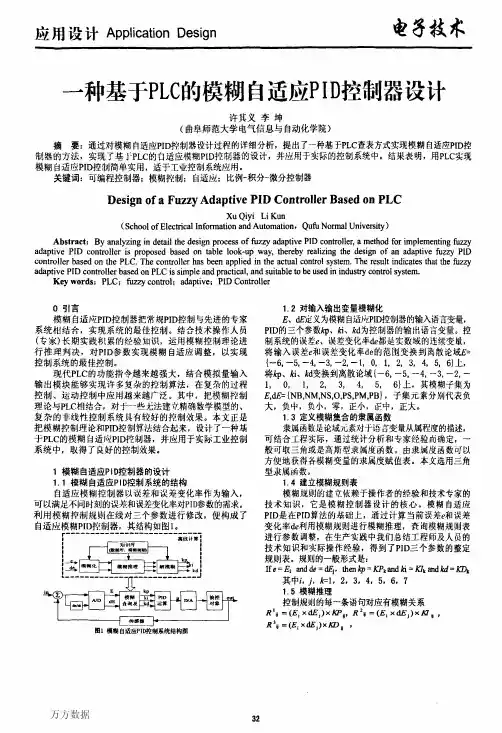
关键词: 模糊控制 自适应 PID PLC中图分类法: TP273 文献标识码: ASelf-adaptive Fuzzy-PID pressure control system based on PLCYANG Yun-fei(Dept. of Information and Control Engineering ,Chang Shu Institute of Technology ,Chang Shu 215500,china ) Abstract : The self-adaptive Fuzzy-PID controller is designed based on traditional PID control technology and fuzzy control technology and it is applied to pressure control system. A self-adaptive Fuzzy-PID control system based on S7-200 PLC is carried out. It takes the deviation and the deviation change as input, according to varying performance state varying the parameters of PID controller to get good dynamic and static control quality. Keywords : Fuzzy control ;adaptive ;PID ;PLC1. 引言常规PID 控制器以其技术成熟在工业控制中得到了广泛的应用,其特点是控制精度高,但鲁棒性差,对非线性、时变参数等系统难以获得满意的控制效果。
113 节能技术与应用示NO.04 2020 W能ENERGY CONSERVATION 基于LabV旧W的模糊自适应PID控制在恒压供水系统中的应用朱多林1韦彪2栗金晶2刘嘉祥2刘欢2(1.长安大学建筑工程学院,陕西西安710061 ; 2.长安大学住房和城乡建设部给水排水重点实验室,陕西西安710061 )摘要:介绍了一种利用L abV丨E W语言设计的基于虚拟仪器的模糊P ID控制系统在恒压供水中的应用利用L ab V IE W的模糊逻辑工具箱(Fuzzy Logic for G T o o lk it)设计模糊自适应P ID控制器,由于其较高的稳定性和自动 优化能力,既能提高系统供水的保障性,又达到了节能的效果。
同时该系统能够实现水压的在线监测和动态分析,并将数据自动保存成表格,可以通过对每天的水压教据分析处理,来不断地改进和优化系统,关键词:Lab V IE W ;模糊P ID控制;虚拟仪器;恒压供水中图分类号:T P273 文献标识码:B文章编号:1004-7948 (2020) 04-0113-03doi : 10.3969/j.issn.l()04-7948.2020.04.034The application of fuzzy adaptive PID control based on Lab V IEW in constant pressure water supplysystemZ H U D u o-l i n W E I B i a o L I Jin-jing et alAbstract :I n t r oduces the application o f a f u z z y P I D control s y s t e m b a s e d o n virtual i n s t r u m e n t d e s i g n e d b y u s i n g L a b V I E W l a n g u a g e in constant pressure w a t e r s u p p l y..B e c a u s e o f its hig h stability a n d a u t omatic optimization ability,i tc a n not o n l y i m p r o v e the s y s t e m w a t e r s u p p l y supportability b ut also a c h i e v e the e n e r g y s a v i n g.A t the s a m e t i m e,thes y s t e m c a n realize the o n-l i n e m o n i t o r i n g a n d d y n a m i c analysis o f w a t e r p r e s s u r e,a n d automatically s ave the data into tables,w h i c h c a n b e c h a n g e d continuously b y analyzing a n d processing the daily w a t e r pressure d ata.Key words :L a b V I E W ;f u z z y P I D ;virtual instrument ;constant pressure w a t e r supply引言由于计算机技术和变频技术的H臻成熟和完善,传 统的高位水箱和压力罐等供水设施逐渐被以变频调速为 核心恒压供水系统所取代。
^信息疼术2016年第11期文章编号= 1009 -2552(2016) 11 -0110-04D O I:10. 13274/j. cnki. hdzj. 2016. 11. 027基于模糊免疫自适应P I D的汽车烘房温度控制系统武斌,赵德安,李在成,蒋佳琳(江苏大学电气信息工程学院,江苏镇江212013)摘要:烘房温度控制是汽车涂装系统的重要环节,对汽车生产的质量、成品率等有重要影响。
针对烘房温度控制系统的难点和性能要求,提出了利用模糊免疫自适应P I D控制器调节烘房温度。
该控制方法兼具模糊控制、免疫控制和传统P I D的优点,通过实时调整P I D控制器的参数来保持系统的稳定性。
仿真结果表明基于自适应模糊免疫P I D控制器在响应速度、抗干扰能力上都优于模糊P I D控制器和传统P I D控制器。
该控制方法为汽车烘房温度控制提供了一种新的控制策略。
关键词:烘房控制系统;模糊控制;免疫控制;PID中图分类号:T P273.5 文献标识码:AD r y i n g o v e n t e m p e r a t u r e c o n t r o l s y s t e m b y u s i n g f u z z yi m m u n e P I D c o n t r o l l e rWU B in,ZHAO De-an,LI Zai-cheng,JANG Jia-lin(School o f Electronic and Inform ation E ngineering,Jiangsu U niversity,Zhenjiang 212013,Jiangsu P rovince,C hina) Abstract :The drying oven temperature control system i s an important component in automobile paintingsystem and also can afiect the automotive production quality,yield and so on.After analyzing the difficulties and performance requirements ol drying oven temperature control,a fuzzy immune adaptive PID control i s presented to adjust temperature ol the drying room.The control method combines the advantages of fuzzy controller,immune controller and the traditional PID controller and maintain the stability of system by adjusting the PID controller parameters.The simulation results showed the fuzzy immune adaptive PID controller in response speed,anti-jamming capability i s superior to the traditional PID controller and the fuzzy adaptive PID controller.The control method provides a new control strategy for automotive drying oven temperature control.Key words:drying oven temperature control system;fuzzy control;immune control;PID0引言据统计烘房能耗占汽车涂装车间能耗的30% 左右,烘炉设备是涂装车间的耗能大户,同时烘房的 功能是实现对车身表面油漆涂层的烘干,涂层的烘 干效果将直接影响车身的外观装饰性和耐腐蚀性,影响到汽车的使用寿命[1-2]。
基于模糊自适应PID的随动系统设计与仿真韩沛;朱战霞;马卫华【期刊名称】《计算机仿真》【年(卷),期】2012(029)001【摘要】The conventional PID controller parameters tuning depends on experience and can not satisfy the high performance. This paper designed a self-adaptive fuzzy PID controller. The parameters of this method can be modi fied online to make the system performance optimal. It used the conventional PID parameters for the initial value, re vised the parameters real-time online through fuzzy and approximated reasoning, thereby enabling the system perform ance to achieve superiorly. It has not only the advantages of flexibility and adaptability of fuzzy control, but also bet ter control precision of PID. In order to verify the self-adaptive fuzzy PID controller's performance, a two-dimension al servo system was taken as the object, which has carried on the simulation in the MATLAB environment and com pared with the conventional PID controller's performance. The result shows that the self-adaptive fuzzy PID controller 's response is superior to the traditional PID controller, and the response speed is faster and more stable precision.%研究随动控制系统优化问题,常规PID控制器参数调试凭经验,导致系统性能不高.为了提高系统快速性和稳定性,提出并设计了模糊自适应PID控制器,可以对参数进行在线修正以使系统性能最优.可采用经验法调试的常规PID参数为初值,再用模糊化和近似推理等对参数进行在线修正,从而使系统性能达到最优.既具有模糊控制灵活性和适应性强的优点,又具有PID 控制精度高的优势.通过设计模糊自适应PID控制器,以某二维随动转台系统为对象,在MATLAB环境中进行了仿真,并与常规PID控制器的性能进行了对比,结果表明模糊自适应PID控制器的响应特性优于传统的PID控制器,响应速度更快,稳态精度更高,为随动系统优化设计提供了依据.【总页数】5页(P138-142)【作者】韩沛;朱战霞;马卫华【作者单位】西北工业大学航天学院,陕西西安710072;西北工业大学航天学院,陕西西安710072;西北工业大学航天学院,陕西西安710072【正文语种】中文【中图分类】TP391.9【相关文献】1.基于温度系统的模糊自适应PID控制器的设计与仿真 [J], 范子荣;张友鹏2.基于提高闭环跟随特性的位置随动系统设计与仿真 [J], 张坤;周浩;3.基于模糊自适应PID控制的反应釜系统的设计与仿真 [J], 罗小燕;于孟;陈斌;蒙鹏宇;4.基于模糊自适应PID控制的反应釜系统的设计与仿真 [J], 罗小燕;于孟;陈斌;蒙鹏宇5.基于模糊自适应PID的连铸二冷控制系统设计与仿真 [J], 刘文红;王彪;马交成;谢植因版权原因,仅展示原文概要,查看原文内容请购买。
摘要随着电力电子技术的发展,作为电能变换装置的DC-DC变换器的应用越来约广泛,隔离式全桥变换器由于高功率,输入输出电气隔离的优点,应用场合广泛,移相控制使得全桥变换器能够实现ZVS软开关工作,进一步减少的变换器的通态损耗,提高了传输效率,广泛应用于对电能质量有着严格要求的航空航天、电力系统等场合中。
本文首先系统地研究了ZVS全桥变换器地具体工作过程,以半个开关周期为例分析了各开关模态的电流回路和持续时间,研究了在ZVS工作时副边整流侧的二极管换向过程,研究了超前桥臂和滞后桥臂各自实现ZVS的条件。
为了验证ZVS工作过程,在Saber仿真软件中搭建了开环仿真模型对开关管的ZVS工作特性进行了验证。
目前,在采用状态空间平均法对全桥电路建模时通常忽略变压器漏感和输出输出滤波电容的ESR,得到的模型并不能准确反映电路自身特性,本文在此基础上提出了一种改进型的小信号模型,该模型包含变压器漏感,输出电容ESR和变换器工作效率等关键参数,并推导了控制到输出及输出阻抗的传递函数,利用Saber搭建仿真模型对模型准确性进行了验证。
针对移相全桥电路的闭环控制和稳定性进行了研究,对电压控制方式和电流控制方式的原理进行了分析,并研究了闭环系统中补偿器的设计流程。
为了提高控制器的性能,在传统PID控制的基础上研究了模糊自适应PID控制方法在全桥变换器中的应用,根据系统输出电压的偏差和偏差的变化率建立模糊规则,在此基础上设计了模糊自适应PID控制器,从而使得PID控制器参数能够动态调整,系统具有更好的动态特性。
为了验证所设计的Fuzzy PID控制器的性能,在Saber和Matlab/Simulink 中搭建了闭环仿真模型,并于传统的PID控制器进行仿真对比。
通过仿真结果的对比可看出,模糊自适应PID控制方式于传统PID方式相比,系统输出电压具有更好的稳定性和动态特性,而且对系统输入电压和负载电阻的大范围变化具有更好的抗干扰性。
1引言近年来电动执行器系统的控制策略得到了越来越多的研究,对系统的稳定运行发挥着关键作用。
电动执行器系统的控制方案主要包括驱动电机以及系统主要单元的控制策略。
系统需要提供相当多的转矩和转速,以控制阀门开度。
对于系统的动态调节,其响应速度应该相对够快,以达到系统控制精度要求。
传统阀门位置控制常采用PID 方法,该方案是基于比例、积分、微分输出控制量,来实现对系统的准确控制,具有相对简单、容易实现等特点。
然而,当被控对象的环境经常变化,即需频繁调整控制参数,对该方法的实际应用提出了限制。
因此,需要对以往的PID 策略进行改进,一种方案是改进传统控制结构,另一种则是采用智能控制方法[1]。
文献[2]研究了PID 控制方案,针对电子液压制动系统下电动执行器调节阀的控制,电动执行器流量调节阀采用传统的控制方法即可实现输出流量精确、快速的跟踪,然而系统具有较差的鲁棒性。
文献[3]采用校正控制,进一步减小了系统超调及稳态误差,大大提升了执行器系统的响应速度和抗扰动能力,并且明显改善了回差。
文献[4]研究了基于增量一种基于模糊自适应PID 的电动执行器智能控制方法李伟华(苏州博睿测控设备有限公司,苏州215143)摘要:电动执行器的系统控制方案研究在近年有较大进展。
传统控制方案基于PID 的控制策略易于在通常的实际控制系统中实现,但对于控制系统复杂程度较高的场合,传统控制方法已不能适应系统鲁棒性和实时性的要求。
为解决此问题,提出基于模糊自适应PID 的执行器系统智能控制方案。
实验结果表明,新方案有较好的动态表现以及较快的响应,并且具有较高的调节准确度,能够实现PID 参数的在线自调整,实时性更好,控制精度和鲁棒性更高,参数计算负荷小,设计方法易于实现。
关键词:模糊控制;自适应;PID 控制;智能控制DOI :10.3969/j.issn.1002-2279.2021.02.015中图分类号:TP273+.4文献标识码:A 文章编号:1002-2279(2021)02-0058-04An Intelligent Control Method of Electric Actuator Based onFuzzy Adaptive PIDLI Weihua(Suzhou Bonray Measurement&Control Equipment Co.,Ltd,Suzhou 215143,China )Abstract:Recently,great progress has been made in the research of system control scheme of electric actuator.The PID-based control strategy of the traditional control scheme is easy to be realized in the common practical control system,but the traditional method can no longer meet the requirements of system robustness and real-time when the control system is complex.To solve the problem,an intelligent control scheme of actuator system based on fuzzy adaptive PID is proposed.Experimental results show that the new scheme has better dynamic performance and faster response,as well as higher adjustment accuracy,which can realize on -line self -adjustment of PID parameters,with better real -time,higher control accuracy and robustness and less parameter calculation load,and the design method is easy to realize.Key words:Electric actuator;Fuzzy control;Self-adaptation;PID control;Intelligent control作者简介:李伟华(1978—),男,陕西省西安市人,助理工程师,主研方向:测控技术及仪器。
类似于pid的控制方法
1. 模糊控制(fuzzy control):模糊控制是一种基于模糊数学理论的控制方法,能够处理具有模糊性质的控制问题。
模糊控制通过模糊规则和模糊推理来实现控制目标。
2. 自适应控制(adaptive control):自适应控制是一种根据系统状态实时调整控制策略的控制方法。
自适应控制可以实现对系统参数、外界干扰和随时间变化的系统参数进行自调节。
3. 预测控制(predictive control):预测控制是一种基于预测模型的控制方式,它通过预测未来的状态和输出来实现控制目标。
预测控制能够处理非线性、非稳态、多变量系统等复杂系统。
4. 逆向控制(inverse control):逆向控制是一种基于目标状态逆推控制策略的控制方法。
逆向控制先确定目标状态,然后通过逆推算法推导控制策略,最终达到控制目标。
5. 强化学习控制(reinforcement learning control):强化学习控制是一种基于智能学习算法的控制方法。
它通过与环境交互,根据奖励机制自主学习最优策略,最终实现控制目标。
采用自适应模糊 PID 的二阶倒立摆控制宋国杰【摘要】建立一个二阶倒立摆的数学模型,将常规比例-积分-微分(PID)控制与模糊控制相结合,设计模糊PID 控制器,实现 PID 参数的自适应模糊整定。
仿真实验表明:所设计的模糊 PID 控制器能很好地实现二阶倒立摆的扶起平衡控制,控制效果明显好于常规 PID 控制器,超调量和调节时间较小,具有较好的抗干扰能力,非常适合二阶倒立摆模型的稳定控制。
%In this paper,a mathematical model of second-order inverted pendulumis built.The conventional proportional-integral-differential (PID)control and fuzzy controlare combined,and a fuzzy PID controlleris designed.The adaptive fuzzy tuning of PID parameters is obtained.Simulation results show the designed fuzzy PID controller can well realize the propped balance control of second-order inverted pendulum,the control effect is obviously better than the conventional PID controller,the overshoot and adjust time is small,and has a good anti-jamming capability.It is very suitable for the stability control of the model of second-order inverted pendulum.【期刊名称】《华侨大学学报(自然科学版)》【年(卷),期】2016(000)001【总页数】5页(P74-78)【关键词】倒立摆;模糊控制;比例-积分-微分控制器;自适应;稳定控制【作者】宋国杰【作者单位】四平职业大学电子工程学院,吉林四平 136002【正文语种】中文【中图分类】TP391.9作为一个典型的不稳定、高阶次、强耦合、多变量非线性系统,倒立摆模型是控制领域内众多专家学者关注和研究的对象[1-2].通过倒立摆模型,可以对已有的控制方法和理论进行模拟和验证,从而提出一些新的理论方法,并将其应用于人工智能、生物工程、计算机视觉、航空航天等领域.目前,对于倒立摆的控制主要包括状态反馈、线性二次型调节器(LQR)等现代控制理论方法,根轨迹、比例-积分-微分(PID)等经典控制理论方法,以及模糊、神经网络、支持向量机等智能方法.其中,PID方法由于理论成熟、便于实现,在倒立摆的控制中应用最为广泛[3-6].尽管如此,PID方法还是存在一些缺陷,如泛化能力差、鲁棒性不高等.除了PID方法,模糊理论也是应用较多的一种方法[7-9].然而,模糊控制方法的适应性较差,当系统参数改变,或出现未知状况时,控制效果明显变差.因此,将两者结合的研究成果也开始出现,但这些研究目前主要集中于一阶或平面倒立摆[10-11].本文将直线二阶倒立摆作为研究对象,将PID控制和模糊控制相结合,设计一种自适应模糊PID控制器.一个典型的直线二阶倒立摆模型主要由小车、两个摆杆和连接块组成[12-13],如图1所示.由于多了一级摆杆,其复杂性远高于一阶倒立摆.首先,根据倒立摆模型的物理学运动规律建立微分方程,即式(1)中:,(m1l1+m2L2)gsin θ1,m1l2gsin θ2]T.其中,m0为小车质量;m1和m2分别为摆杆1和摆杆2的质量;J1和J2分别为摆杆1和摆杆2的转动惯量;l1和l2分别为摆杆1和摆杆2转动中心到杆质心的距离;L1和L2分别为摆杆1和摆杆2的长度;f0为小车与轨道间的摩擦系数;f1和f2分别为摆杆1和摆杆2的绕动摩擦系数;g为重力加速度.对式(1)在系统平衡点处进行线性化处理,可得系统的状态方程为式(2)中:;Y=[r,θ1,θ2]T;;;C=[I3,03];;0和I分别表示适当维数的零矩阵和单位阵.至此,可以得到直线二阶倒立摆的状态空间方程.在设计控制器时,考虑将PID算法和模糊算法有机结合,既利用前者的实用性,又结合后者的智能性.根据对二阶倒立摆模型参数和稳定条件的分析,在设计模糊推理时,采用Mamdani的形式,通过在线方式实时调节PID算法的3个参数[13-14].具体思路为:将一个常规PID控制器作为主控制器,另设计一个模糊推理模块,利用该模块对PID控制器的比例、积分和微分3个参数进行自适应整定.此外,文中进行了两点改进.1) 以往大多数的模糊推理模块只是单纯地将偏差E作为输入,为了更为客观、迅速地反映系统变化,将偏差变化率CE也作为一个输入.2) 设计模糊推理模块的输出为参数的变化调整量,则PID算法只需进行相应的调整即可.这样模糊推理模块就形成了一个2输入、3输出的结构,具体如图2所示.由图2可知:该控制器结构同时具有PID和模糊两种算法的优点,其动态和静态性能较好,非常适合二阶倒立摆这样的非线性动态系统控制.根据设计的模糊PID控制器的结构,将二阶倒立摆的摆杆1和摆杆2所在的角度偏差E及其变化率CE作为系统输入.设定角度偏差E和偏差变化率CE的模糊子集为{负大,负中,负小,零,正小,正中,正大},利用符号表示为{NB,NM,NS,Z,PS,PM,PB},输出模糊子集与其具有相同形式的符号表示.根据E和CE对系统影响程度的不同,当变化超过60%时,即达到了模糊推理模块的最大值,故设定E和CE基本论域分别为[-80,80],[-10,10],输入量的模糊论域为[-6,6];3个输出变量ΔKP,ΔKI和ΔKD的基本论域为[-0.4,0.4],[-0.06,0.06],[-3, 3],模糊论域为[-3,3].考虑到等三角函数的灵敏度较高,可以在论域范围内均匀分布,故将其作为隶属度函数.据此,对PID算法的比例 KD、积分KI、微分KD等3个参数制定不同情况下的整定规则.1) 当角度偏差E变化较大时,很可能出现微分过饱现象,使系统超出控制范围.为了保证系统能够快速响应,KP应设定为一个较大数值,KD相应的需设定较小一些,同时取KI,防止系统超调过大.2) 当角度偏差E和偏差变化率CE的值在适中范围时,既要考虑系统的超调不能过大,又要保证系统具有较快的响应速度,KP需设定一个较小的数值,KI和KD取值适中即可.3) 当角度偏差E变化较小时,首先,需要让系统维持较好的稳定性,KP和KI都应设定较大的数值;其次,考虑降低系统振荡的风险,KD应与角度偏差变化率CE 的取值进行相反设定.针对比例KP、积分KI、微分KD等3个参数的模糊控制规则,分别如表1~3所示.对提出的模糊PID控制器的二阶倒立摆控制性能进行仿真分析,并与文献[4]提出的PID方法进行对比.利用Matlab软件的Simulink模块,搭建PID控制算法的系统,结果如图3所示.这3个PID控制器分别控制小车位移r和两个摆杆的角度α1和α2[15].对于二阶倒立摆这样的典型不稳定系统,初始值的不同对于PID算法的控制效果具有很大的影响,选择不当会使控制品质下降,甚至系统发散.选择两组初始参数,分别设定为 (r,α1,α2)={0,0,0},(r,α1,α2)={-0.1,-0.2,-0.1},控制效果如图4所示.由图4可知:PID方法对于二阶倒立摆具有一定的控制效果,要求系统初始参数选择适当;第一组参数明显具有更短的调节时间,但第二组参数的超调量更小.此外,PID方法的3个参数也需根据经验或经过多次反复试验给定,泛化性较差.其次,根据设计的模糊PID控制器搭建系统模型,将图3中的3个常规PID控制器替换为图5所示的模糊PID控制器即可,其他不变.在仿真过程中,仍取上述相同的两组初始条件,仿真结果如图6所示.由图6可知:模糊PID对于二阶倒立摆具有较好的控制效果.相较于常规PID方法,模糊PID降低了系统对于初始值的敏感度,两组参数情况下的控制效果相当,超调量和调节时间都明显较小,且明显好于常规PID方法.最后,在程序编译成功之后,采用手动方式将摆杆提到中间的一个平衡位置,运行程序,其控制效果如图7,8所示.由图7,8可知:模糊PID方法对于二阶倒立摆系统控制的稳定度明显高于常规PID 方法,两个摆杆角度的变化幅度也明显较小.多次改变系统初始参数,控制效果基本相同,这里不一一赘述.在系统运行过程中,突然施加一个外部扰动,考察模糊PID方法的抗干扰性,控制结果如图9所示.由图9可知:在系统运行第3 s时,突然受到一个外部干扰,但是在大概2 s以后就迅速恢复为稳定状态,而且系统的超调量较小,说明模糊PID方法对于外部扰动具有较好的抑制作用.综合比较以上结果可知,所设计的模糊PID控制器对二阶倒立摆具有较好的控制效果,无论是超调量,还是调节时间都明显好于常规PID方法.采用自适应模糊PID对直线二阶倒立摆的控制问题进行研究.首先,建立二阶倒立摆的数学模型,反映出其是一个典型的不稳定系统;其次,将常规PID算法与模糊理论相结合,设计模糊PID控制器,可以实现PID参数的自适应模糊整定[16].仿真及实测实验表明:所设计的模糊PID控制器可以很好地实现二阶倒立摆的扶起平衡控制,控制效果明显好于常规PID控制器,超调量和调节时间较小,并具有较好的抗干扰能力,为直线二阶倒立摆的控制问题提供了一条可借鉴的思路.【相关文献】[1] 赵建军,魏毅,夏时洪,等.基于二阶倒立摆的人体运动合成[J].计算机学报,2014,37(10):2187-2195.[2] 吴震宇,方敏,丁康.基于LabVIEW的二级倒立摆控制系统三维仿真[J].合肥工业大学学报(自然科学版),2011,34(10):1480-1484.[3] 项雷军,王涛云,郭新华.多区域互联电网的分散式模糊PID负荷频率控制[J].华侨大学学报(自然科学版),2014,35(2):121-126.[4] 杨平,徐春梅,贺茂康,等.直线二级倒立摆的PID实时控制[J].上海电力学院学报,2008,24(3):236-238.[5] 王宏楠.基于RBF神经网络二级倒立摆系统的PID控制[J].辽宁石油化工大学学报,2010,30(2):58-61.[6] 王俊.基于倒立摆的PID控制算法的研究[J].现代电子技术,2012,35(23):152-154.[7] 李红伟.单级倒立摆的简化模糊控制及仿真研究[J].控制工程,2010,17(6):769-773.[8] 侯涛,牛宏侠.平面一级倒立摆的双闭环模糊控制研究[J].兰州交通大学学报,2011,30(4):11-19.[9] 侯涛,范多旺,杨剑锋.基于T-S型的平面倒立摆双闭环模糊控制研究[J].控制工程,2012,19(5):753-756.[10] 王子涛,王家军,何杰.基于自适应模糊PID平面倒立摆的建模与仿真[J].杭州电子科技大学学报,2010,30(4):86-91.[11] 杨治明,宋乐鹏,杨清林,等.基于模糊控制和PID控制的一阶倒立摆系统建模与仿真[J].北华大学学报(自然科学版),2012,13(3):356-359.[12] 洪江,周明华.二阶倒立摆的稳定性控制[J].科技资讯,2012,36(27):70-71.[13] 王春民,栾卉,杨红应.倒立摆控制的设计与仿真[J].吉林大学学报(信息科学版),2009,6(3):242-247.[14] 王广雄,张静,罗晶,等.倒立摆的模型和控制问题[J].电机与控制学报,2004,8(3):247,262-295.[15] 柴军营,何广平.倒立摆的一种新的控制方法[J].北方工业大学学报,2007,4(3):26-30.[16] 李贤涛,张葆,赵春蕾,等.基于自适应的自抗扰控制技术提高扰动隔离度[J].吉林大学学报(工学版),2015,6(1):202-208.。
收稿日期:2004-03-31第22卷 第9期计 算 机 仿 真2005年9月文章编号:1006-9348(2005)09-0242-03模糊自整定PID 控制器设计以及MATLAB 仿真分析肖奇军1,李胜勇2(1.肇庆学院电子信息工程系,广东肇庆526061;2.上海交通大学微纳米科学技术研究院,上海200030)摘要:为了解决液压控制的关键技术,该文针对时变、非线性的电液伺服系统提出了模糊自整定PID 控制器设计的思路,结合Simuiink 和模糊工具箱并进行仿真分析,该仿真模型具有结构简单、界面直观、便于修改等特点,根据PID 参数变化需要提出了模糊控制规则选取方法,给出了系统软、硬件实现方法,该系统具有操作方便、人机界面风格良好等优点。
使用仿真和实验相结合的方法获取最佳控制参数,通过仿真和实验结果可以看出这种算法的实用性和有效性。
关键词:模糊自整定;仿真分析;应用分析;电液伺服系统中图分类号:TP391.9 文献标识码:B Design and Simulation Analysis of Fuzzy Self -adaptive PID ControlXIAO Oi -jun 1,LI Sheng -yong 2(1.Dept.of Eiectronics Information Engineering ,Zhaoging University ,Zhaoging Guangdong 526061,China ;2.Institute of Micronanometer Science and Technoiogy Shanghai Jiaotong Univ.,Shanghai 200030,China )ABSTRACT :The paper puts forward the idea of fuzzy seif -adaptive PID controiier design aimed at the time -chan-ging and non -iinear eiectro -hydrauiic servo and the simuiation anaiysis combined with Simuiink and fuzzy tooibox.The simuiation possesses the characteristic of simpie construction ,direct interface and easy modification etc and ob-tains the way for fuzzy controi ruie seiection according to the need of PID parameter changing.It aiso provides the way for software and hardware reaiization.The system possesses the merit of convenient operation and good interface.It ob-tains the best parameter through simuiation combined with experience and from the simuiation resuit we can see the practicaiity and vaiidity of this controi method and soive the key technoiogy of hydrauiic controi.KEYWORDS :Fuzzy seif -adaptive ;Simuiation anaiysis ;Appiication anaiysis ;Eiectro -hydrauiic servo1 引言模糊控制一直是智能控制研究的热点,其应用水平代表着产品智能化水平,模糊控制以其控制简单、实现成本低廉、无需建立数学模型等独到的优点被广泛应用于家电等控制中,尤其是在时变、非线性的液压控制系统中得到广泛的应用。
Research ArticleA fuzzy model based adaptive PID controller design for nonlinearand uncertain processesAydogan Savran n,Gokalp Kahraman1Department of Electrical and Electronics Engineering,Ege University,35100Bornova,Izmir,Turkeya r t i c l e i n f oArticle history:Received19September2012Received in revised form16September2013Accepted26September2013Available online17October2013This paper was recommended forpublication by Prof.A.B.RadKeywords:AdaptivePIDFuzzyPredictionSoft limiterLMBPTTControla b s t r a c tWe develop a novel adaptive tuning method for classical proportional–integral–derivative(PID)controller to control nonlinear processes to adjust PID gains,a problem which is very difficult toovercome in the classical PID controllers.By incorporating classical PID control,which is well-known inindustry,to the control of nonlinear processes,we introduce a method which can readily be used by theindustry.In this method,controller design does not require afirst principal model of the process which isusually very difficult to obtain.Instead,it depends on a fuzzy process model which is constructed fromthe measured input–output data of the process.A soft limiter is used to impose industrial limits on thecontrol input.The performance of the system is successfully tested on the bioreactor,a highly nonlinearprocess involving instabilities.Several tests showed the method's success in tracking,robustness to noise,and adaptation properties.We as well compared our system's performance to those of a plant withaltered parameters with measurement noise,and obtained less ringing and better tracking.To conclude,we present a novel adaptive control method that is built upon the well-known PID architecture thatsuccessfully controls highly nonlinear industrial processes,even under conditions such as strongparameter variations,noise,and instabilities.&2013ISA.Published by Elsevier Ltd.All rights reserved.1.IntroductionPID controllers are well-known and popular in industry due totheir simplicity and robustness,but most of them lack well-tuningand accuracy,that motivated much work to develop tuning andadaptation techniques to cope with nonlinear industrial processes[1–8].Adaptive tuning becomes necessary for parameter varia-tions,whichfixed parameter controllers cannot sufficiently com-pensate.Recently,predictive control technique has been widelyappeared in the process control[9–11].In the predictive control,aprocess model is required to predict the future effects of thecontrol action at the present.First principles-based nonlinearmodels are difficult to develop for many industrial cases.Non-linear process can be alternatively modeled with fuzzy systems.Fuzzy logic was introduced by Zadeh[12,13]and then used formany control and modeling applications[14,15].Takagi–Sugeno[16]and Mamdani[17]fuzzy models are the two main types offuzzy systems.The Takagi–Sugeno fuzzy model(Takagi–Sugenomodeling methodology)includes fuzzy sets only in the premisepart and a regression model as the consequent[16]while theMamdani fuzzy model includes fuzzy sets in both parts.Manysuccessful applications of the predictive control using fuzzymodels have been reported in the literature[18–21].Although,the PID tuning and adaptation techniques have exten-sively developed for linear time-invariant systems[2,3,22–26],still much effort should be spent for nonlinear as well as time-variant systems.This has motivated this study.In this paper,anovel adaptive tuning procedure for classical PID controllers isdeveloped and efficiently applied for a nonlinear process controlproblem.One of the main features of the proposed approach isthat the PID controller architecture is solely classic making itreadily usable in nonlinear industrial processes,avoiding lengthyand less familiar fuzzy systems.Our classic PID design allowscomputing the parameters from the measured input–output dataof the nonlinear process more precisely than other known designsby virtue of its multi-step forward prediction,on-line predictortraining,adaptive controller tuning,and fast training features.Bythis way,a predictive adjustment procedure is performed based onthe predictions of a fuzzy model of the process.Adaptation partinvolves a classical PID controller driving a fuzzy predictor.Thefuzzy predictor output is used to adjust the gains by minimizing theerror between the predictions and the reference.Additionally,thefuzzy predictor is trained on-line to adapt to the variations in plantparameters,and thus improve the prediction accuracy.The actualplant is controlled by a PID controller identical to that of theContents lists available at ScienceDirectjournal homepage:/locate/isatransISA Transactions0019-0578/$-see front matter&2013ISA.Published by Elsevier Ltd.All rights reserved./10.1016/j.isatra.2013.09.020n Corresponding author.Tel.:þ902323111664;fax:þ902323886024.E-mail addresses:aydogan.savran@.tr(A.Savran),gokalp.kahraman@.tr(G.Kahraman).1Tel.:þ902323111669;fax:þ902323886024.ISA Transactions53(2014)280–288adaptation part,the gains of which are transferred at each control cycle.A soft limiter is used to impose industrial limits on the control input.In a concurrent work[27],we have used a fuzzy system to implement the controller that resulted in procedurally lengthy and computationally heavy algorithms that are unfavorable in industrial users.In contrast,in this work simple PID gain parameters replace lengthy fuzzy-system computations.The predictor is constructed only from the measurement of the input–output data of the actual process as a fuzzy model,without requiring afirst-principal model of the process which is usually very difficult to obtain.Section2provides background information on the structure of the fuzzy systems and the PID controller,used in the paper, whereas Section3explains the control system architecture and the training procedure.Section4discusses the results of the performance tests done on the bioreactor,a highly nonlinear process involving instabilities.Several tests and comparative study showed the method's success in tracking,robustness to noise,and adaptation properties.Section5is the conclusion,summarizing the performance of our method.2.The background2.1.The PID controllerProportional–integral–derivative(PID)controllers,which have relatively simple structures and robust performances,are the most common controllers in industry.By taking the time-derivative of the both sides of the continuous-time PID equation,and discretiz-ing the resulting equation,one easily gets the PID equation in the incremental form as below:uðkÞ¼uðkÀ1ÞþK PðeðkÞÀeðkÀ1ÞÞþK I T2ðeðkÞþeðkÀ1ÞÞþK DTðeðkÞÀ2eðkÀ1ÞþeðkÀ2ÞÞð1Þwhere K P is the proportional gain,K I is the integral gain,and K D is the derivative gain.T is the sampling period,u is the output of the PID controller,and k is the discrete time index.The difference between the reference input(r)and the actual plant output(y)is the error term,e¼rÀy.Equation can be simplified toΔuðkÞ¼K P e PðkÞþK I e IðkÞþK D e DðkÞuðkÞ¼uðkÀ1ÞþΔuðkÞð2Þwheree PðkÞ¼eðkÞÀeðkÀ1Þe IðkÞ¼T2ðeðkÞþeðkÀ1ÞÞe DðkÞ¼1ðeðkÞÀ2eðkÀ1ÞþeðkÀ2ÞÞð3Þwith eðkÞ¼0for k o0.In order to provide the control signal in physical limits,a soft limiter is placed after the controller.The control signal at the output of the soft limiter becomesu lðkÞ¼hðuðkÞÞð4Þwhere hðuÞ¼1=1þeÀu is a sigmoid type function.2.2.The fuzzy systemThe fuzzy system(FS),fðx;θÞ,used in this study consists of the product inference engine,the singleton fuzzifier,the center average defuzzifier,and the Gaussian membership functions[28,29]:fðxðkÞ;θÞ¼∑Mj¼1b j∏N i¼1expðÀ12ðx iðkÞÀc ij=s ijÞ2Þ∑Mj¼1∏Ni¼1expðÀ12ðx iðkÞÀc ij=s ijÞ2Þð5Þwhere x i is the i th input of the FS,N is the number of inputs,M is the number of membership functions assigned to each input,c ij and s ij are,respectively,the center and the spread of the j th membership function corresponding to the i th input.Any output membership function which has afixed spread of1is characterized only by the center parameter b j.The input vector x(k)represents all of the inputs of the FS at time k.The parameter vectorθ¼½b;c;r contains all of the fuzzy-set parameters.The derivativesð∂fðxðkÞ;θÞ=∂θÞfor the FS output with respect to its parameters are computed as∂f∂b j¼∂f∂α∂α∂b j¼1ϕz j∂f∂c ij¼∂f∂z j∂z j∂c ij¼ðb jÀfÞϕz jðx iÀc ijÞðs ijÞ2∂f∂s ij¼∂f∂z j∂z j∂s ij¼ðb jÀfÞϕz jðx iÀc ijÞ2ðs ijÞð6Þwherez j¼∏N i¼1expðÀ12ðx iÀc ij=s ijÞ2Þα¼∑M j¼1b j z jφ¼∑M j¼1z jf¼αφð7ÞThe input–output sensitivities of the FS are computed as∂fðxÞ∂x i¼∑M j¼1fðxÞÀb jφz jx iÀc ijs2ij!ð8Þ3.The adaptive PID control system3.1.Control system architectureFig.1depicts the adaptive PID control system architecture.The adaptation part includes the PID controller and the fuzzy predictor. The PID controller computes the control actions.The predictor is constructed only from the measurement of the input–output data of the actual process as a fuzzy model,without requiring afirst-principal model of the process which is usually very difficult to obtain.The multi-step ahead predictions of the process output are provided by the fuzzy predictor.The fuzzy predictor output is used to adjust the gains by minimizing the sum of the squared errors between the predictions and the reference over the prediction horizon.The fuzzy predictor is trained on-line to adapt to the variations in plant parameters,and thus improve the prediction accuracy.A certain history of the actual plant inputs and outputs is stored in afirst-infirst-out stack,providing the online training data at each training step[30].The PID controller gains and the predictor fuzzy system parameters are both adjusted by the Levenberg–Marquardt(LM)method[31].The actual plant is controlled by a PID controller identical to that of the adaptation phase,the gains of which are transferred at each control cycle.A sigmoid-type soft limiter is used to impose industrial limits on the control input.3.2.Adaptation of the PID controller gainsThe fuzzy predictor parameters and the controller gains are adjusted at each control cycle.The cost function used to adjust the controller gains is defined as the sum of the squared errorA.Savran,G.Kahraman/ISA Transactions53(2014)280–288281between the set point and the predictor output over the prediction horizon H as below:E H c ¼12H∑HÀ1n¼0ðrðkþnÞÀ^yðkþnÞÞ2ð9Þwhere k is the initial edge of the prediction horizon.The Jacobian with respect to the controller gainsθc¼½K p;K I;K D is computed asJ c¼∂^e∂θc¼∂^e∂f p∂f p∂^l∂^u l∂^∂^u∂θcð10ÞOne should notice that the delay elements at the outputs of PID controller and the fuzzy predictor form recurrent systems,and as such their Jacobians(or equivalently gradients)are computed by the back-propagation through time(BPTT)method which is based on the adjoint model.The JacobiansðJ c¼∂^e=∂θcÞare computed in two phases referred as the forward and the backward.In the forward phase,at every time step k,the controller and predictor sequentially run and their outputs are stored from n¼0to n¼HÀ1,where n counts the ahead of time steps and H is the prediction horizon.The ahead-of-time value of control signal,denoted as^uðnÞ,drives the predictor, and it is given by^uðnÞ¼^uðnÀ1ÞþΔ^uðnÞ;for n¼0;1;:::;HÀ1ð11ÞwhereΔ^uðnÞ¼K P^e PðnÞþK I^e IðnÞþK D^e DðnÞð12Þ^e pðnÞ¼^eðnÞÀ^eðnÀ1Þ^e IðnÞ¼Tð^eðnÞþ^eðnÀ1ÞÞ^e DðnÞ¼1Tð^eðnÞÀ2^eðnÀ1Þþ^eðnÀ2ÞÞð13ÞThe difference between the reference and the predictor output, ^eðnÞ¼rðkþnÞÀ^yðkþnÞis the ahead-of-time error.The initial con-ditions of the equations from(11)to(12)are^uðn¼À1Þ¼uðkÀ1Þ^eðn¼0Þ¼eðkÀ1Þ,^eðn¼À1Þ¼eðkÀ2Þ,and^eðn¼À2Þ¼eðkÀ3Þ.The control action at the output of the limiter is obtained as^ulðnÞ¼hð^uðnÞÞ;ð14Þwhere limiter h is a sigmoid type function.The predictor input vector contains the control action and the previous predictor output:^x pðnÞ¼½^yðkþnÀ1Þ;^ulðnÞ ð15ÞThe predicted plant output is the predictor output:^yðkþnÞ¼fp ð^x pðnÞ;θpÞð16Þwhere the parameter vectorθp¼½b p;c p;r p contains all of thefuzzy-set parameters of the predictor.The mean square error through the prediction horizon iscomputed asE Hc¼1∑HÀ1n¼0^e2ðnþ1Þð17ÞTable1summarizes the forward phase computations.At the completion of the forward phase at each k,the backwardphase computations from n¼HÀ1to n¼0are performed bymeans of the adjoint model shown in Fig.2.In the adjoint model,the arrow directions of the signal propagation are reversed,thesumming junctions and the branching points are interchanged,and the advance operators replace the delay operators.The backward action at the predictor output is obtained asδpðnÞ¼½À1þvðnþ1Þ ;for n¼HÀ1;:::;0:ð18Þwith vðn¼HÞ¼0.The vðnÞis computed viaδpðnÞ:vðnÞ¼∂f pðx p;θpÞp1^x pðnÞδpðnÞð19ÞThe backward action at the limiter input is obtained asδlðnÞ¼½hð^uðnÞÞ∂f pðx p;θpÞ∂x p2^x pðnÞδpðnÞð20ÞTable1The forward phase computations.θc¼½K p;K I;K Dθp¼½b p;c p;r p^eð0Þ¼rðkÀ1ÞÀyðkÀ1Þn¼0;:::;HÀ1^e pðnÞ¼^eðnÞÀ^eðnÀ1Þ^e IðnÞ¼Tð^eðnÞþ^eðnÀ1ÞÞ^e DðnÞ¼1Tð^eðnÞÀ2^eðnÀ1Þþ^eðnÀ2ÞÞΔ^uðnÞ¼K P^e PðnÞþK I^e IðnÞþK D^e DðnÞ^uðnÞ¼^uðnÀ1ÞþΔ^uðnÞ^ulðnÞ¼hð^uðnÞÞ^x pðnÞ¼½^ulðnÞ;^yðkþnÀ1Þ^yðkþnÞ¼fpð^x pðnÞ;θpÞ^eðnþ1Þ¼rðkþnÞÀ^yðkþnÞE H c¼1∑HÀ1n¼0^e2ðnþ1ÞFig.1.Proposed PID control system architecture.A.Savran,G.Kahraman/ISA Transactions53(2014)280–288282where h ′ð^u ðn ÞÞ¼∂h =∂u j u ðn Þ¼^u ðn Þis the derivative of the limiter function with respect to its input.The backward action at the controller output is obtained as δc ðn Þ¼δl ðn Þþδc ðn þ1Þð21Þwith δc ðn ¼H Þ¼0.The Jacobian with respect to the controller gains is calculated by J c ðn Þ¼∂^e ðn Þ∂θc ¼δc ðn Þ∂Δ^uðn Þ∂θcð22ÞWhere the derivative ð∂Δ^u=∂θc Þis obtained as ∂Δ^u ðn Þ∂θc ¼∂Δ^uðn Þ∂K p ;∂Δ^u ðn Þ∂K I ;∂Δ^u ðn Þ∂K D¼½^e p ðn Þ;^e I ðn Þ;^e D ðn Þ ð23ÞTable 2summarizes the backward phase computations.The PID controller gains are updated based on the elements ofthe Jacobian matrix ðJ c ¼∂^e=∂θc Þ.The change in parameter vector,Δθc ,of the controller follows fromðJ T c J c þμI ÞΔθc¼ÀJ T c ^eð24Þby the LM method.Here μis a positive constant,I is the identity matrix,and the superscript T denotes transpose.For a suf ficientlylarge value of μ,the matrix ðJ T c J c þμI Þis positive de finite,and Δθcdescribes a descent direction.μis determined with a trust region approach.A detailed description of the LM with the trust region approach is given in [32].The computations are repeated for a certain iteration number at each stage to reduce the predicted tracking error to a suitable level.The adjusted controller gains are transferred to the controller of the application part which gen-erates the control action to apply to the actual plant.Then the next stage of the adaptation process is started.3.3.The predictor trainingThe predictor is a recurrent system using the FS de fined by Eq.(5),and as such its Jacobian is computed by the back-propagation through time (BPTT)method.It can be trained off-line to accurately represent the process dynamics by using the input –output data of the process.An on-line training procedure is used to adapt tothe changes in process dynamics (Fig.3).In this procedure,a shorthistory of the training data is stored in a first-in first-out stack of depth (L ),where the oldest data is discarded,and the newest is entered.The stack length L is chosen to suf ficiently represent as well as adapt the system dynamics,eliminating the too old data while keeping the recent changes.The on-line training is performed using the stack data at each time step.The training of the predictor corresponds to adjustingthe FS parameters,θp ¼½b p;c p ;r p .The cost function at each time step k is the mean square error (MSE)between the actual plantoutputs ðy p Þand the predictor outputs ð^y Þin the stack,given by E L m ¼12L ∑Ll ¼1½y pðl ÞÀ^yðl Þ 2ð25Þwhere k is omitted for brevity.4.Illustrative benchmark example:the bioreactor control The performance of the proposed control method is demon-strated on a nonlinear bioreactor benchmark problem [33],used in Refs.[34–36],since the strong nonlinearities and instabilities in bioreactor dynamics present a challenge for control.The bioreac-tor tank contains water in which nutrients and biological cells mix.The constituents of the tank are kept at a constant volume by keeping in flow and out flow rates equal to the same control input variable,u .The dimensionless state variables of the process,x 1and x 2,are the amount of cells and nutrients in the tank,respectively.Coupled nonlinear differential equations describing the bioreactor process aredx 1dt ¼Àx 1u þx 1ð1Àx 2Þe x 2=γdx 2dt¼Àx 2u þx 1ð1Àx 2Þe x 2=γð1þβÞ=ð1þβÀx 2Þð26Þwhere 0r x 1,x 2r 1,and 0r u r 2.The constant parameters γand βdetermine the rates of cell formation and nutrient consumption,respectively.For the nominal benchmark speci fication,they are set as γ¼0.48and β¼0.02[33,34].The simulation data sets are obtained by integrating Eq.(26)by a fourth-order Runge –Kutta algorithm using an integration step size of Δ¼0.01time units.We de fine 50Δas the macro time step.We first construct the predictor through the task of designing our adaptive PID control system.In the bioreactor problem,theFig.2.The adjoint model of the adaptation part.Table 2The backward phase computations.n ¼H À1;:::;0δp ðn Þ¼½À1þv ðn þ1Þ with v ðn ¼H Þ¼0v ðn Þ¼∂f p ðx p ;θp Þp 1^x p ðn Þδp ðn Þh ′ð^u ðn ÞÞ¼∂h ∂uu ðn Þ¼^u ðn Þδl ðn Þ¼½h ′ð^u ðn ÞÞ ∂f p ðx p ;θp Þ2^xp ðn Þδp ðn Þδc ðn Þ¼δl ðn Þþδc ðn þ1Þwith δc ðn ¼H Þ¼0∂Δ^u ðn Þc ¼∂Δ^uðn Þp ;∂Δ^u ðn ÞI ;∂Δ^u ðn ÞD¼½^ep ðn Þ;^e I ðn Þ;^e D ðn Þ J c ðn Þ¼∂^e ðn Þc ¼δc ðn Þ∂Δ^uðn ÞcFig.3.The on-line predictor training.A.Savran,G.Kahraman /ISA Transactions 53(2014)280–288283predictor fuzzy system(FS)has2inputs(N¼2)and6rules(M¼6). The stack size L and the prediction horizon H are both set to5. Initially,the Gaussian membership functions with equal spread are used,and their centers are equally placed to cover the entire domain.One of the fuzzy membership functions before and after training is shown in Fig.4.The performance of the predictoris Fig.4.The fuzzy membership function before and aftertraining.Fig.5.The outputs of the plant and the fuzzypredictor.Fig.6.Instantaneous error with respect to k.Fig.7.The control system response in the stable(k o100)and unstable(k4100)regions.Fig.8.The trajectory of the uncontrolled statex2.Fig.9.The control input.A.Savran,G.Kahraman/ISA Transactions53(2014)280–288284depicted in Figs.5and 6,where the plant output is estimated very closely with an off-line mean-square-error of 2.65Â10À7.4.1.Control of the bioreactor in stable and unstable regions We tested the performance of the control system for the nominal plant parameters (γ¼0.48and β¼0.02).A sigmoid type limiter is considered to provide control input limits for the bioreactor.The limiter function is 2h ðu Þ¼2=ð1þe Àu Þ,since the bioreactor control input must be between 0and 2.We deal with the bioreactor control problem speci fied as the hardest by Ref.[33].In this problem,the desired state is first set to a stable valueðx n1;x n 2Þ¼ð0:1237;0:8760Þwith u n¼1=1:3.Then,after 100microtime steps (50s),0.05added to x n1giving x n1¼0:1737.This shiftsthe set point from the stable region to the unstable region.The PID gains at the end of the simulation are obtained as ðK p ;K I ;K D Þ¼ðÀ22:9408;À16:0045;À1:6895Þ.The performance of our PID control system for this problem is shown in Figs.7–9.The set points in both stable and unstable regions are satisfactorily tracked,where a mean square error of 2Â10À5is obtained.4.2.Robustness to noiseThe performance of the control system by injecting noise on the state variables is also demonstrated.This is performedbyFig.10.The control system response undernoise.Fig.11.The trajectory of the uncontrolled state x2undernoise.Fig.12.The controlinput.Fig.13.The lack of adaptation of the control system with the fixed gains.The system parameters change at k ¼400.Fig.14.The trajectory of the uncontrolled state x2under fixed gains.A.Savran,G.Kahraman /ISA Transactions 53(2014)280–288285adding the white Gaussian noise with a standard deviation of 0.001to the state variables.The performance of the control system is depicted in Figs.10–12.The control system sufficiently tracks the reference,showing the robustness to noise.4.3.Adaptation performanceThe adaptation is tested by altering the bioreactor parameters γ¼0.48to0.456(5%)andβ¼0.02to0.016(20%)at the time indexof400.We performed simulations using the controller the gains of which arefirstlyfixed to their off-line trained valuesðK p;K I;K DÞ¼ðÀ22:9408;À16:0045;À1:6895Þwith(γ¼0.48andβ¼0.02),andsecondly are adaptively on-line trained.Figs.13to15show the lack of adaptation to the system parameter change at k¼400in the first case.The same simulation is carried out using the adaptive PID controller.The same initial values for the gainsðK p;K I;K DÞ¼ðÀ22:9408;À16:0045;À1:6895Þare used as in thefixed case.In this case,the gains continue to update.The variation of the PID controller gains with adaptation is shown in Fig.16.Note that in both nominal(k o400)and altered(k4400)parameter regions, system is nonlinear but with a different set of parameters.Thus, the parameter change in the process is successfully compensated as shown in Figs.17–19.The overall mean-squared-error(MSE) obtained is1.5Â10À4.parative studyThe performance of the proposed control system is tested by comparing the two of the problems,namely“the nominal plant parameters(γ¼0.48andβ¼0.02)”and“a plant with altered parameters(γ¼0.456andβ¼0.016)with Gaussian measurement noise with a standard deviation of0.01”both“with limited state information”studied on pages291and292in Ref.[34].The reference trajectory is taken fromfigures12and14of Ref.[34]. Since only the state x1(the amount of cells)is used to design the controller and the predictor,our design relates to the limited-state problems stated in[34].Firstly,the performance of the controller is tested with the nominal parameters.The performance of our system is depicted in Figs.20–22.Our result has less ringing in the controlled state when compared with the corresponding results infigure12of Ref.[34].We calculated the MSE as1.95Â10À4.Fig.15.The control input underfixedgains.Fig.16.The variation of the PID controller gains withadaptation.Fig.17.The control system response for the nominal(k o400)and altered(k4400)system parameters.Note that in both regions system is nonlinear butwith a different set ofparameters.Fig.18.The trajectory of the state x2with the nominal(k o400)and altered(k4400)parameters.A.Savran,G.Kahraman/ISA Transactions53(2014)280–288286。