Distribution of magnetic domain pinning fields in GaMnAs ferromagnetic films
- 格式:pdf
- 大小:222.68 KB
- 文档页数:14

物理专业英语词汇(M)Favorite m center m 中心mach angle 马赫角mach cone 马赫锥mach number 马赫数mach wave 马赫波mach zehnder interferometer 马赫曾德耳干涉仪mach's principle 马赫原理machine language 机骑言machine oriented language 面向机颇语言macleod gage 麦克劳计macro crystal 粗晶macrography 宏观照相术macroinstability 宏观不稳定性macromolecule 高分子macron 宏观粒子macroparticle 宏观粒子macrophysics 宏观物理学macroscopic brownian motion 宏观布朗运动macroscopic particle 宏观粒子macroscopic quantization 宏观量子化macroscopic system 宏观系统macrostate 宏观态macrostructure 宏观结构macrosystem 宏观系统magdeburg hemispheres 马德堡球magellanic clouds 麦哲伦星系magellanic galaxy 麦哲伦星系magic eye 光党指示管magic lantern 幻灯magic number 幻数magic t t 形波导支路magma 岩浆magneli structure 马格涅利结构magnesium 镁magnet 磁铁magnetic 磁的magnetic amplifier 磁放大器magnetic analyzer 磁分析器magnetic anisotropy 磁蛤异性magnetic anomaly 磁异常magnetic axis 磁轴magnetic balance 磁力天平magnetic birefringence 磁双折射magnetic breakdown 磁哗magnetic bubble 磁泡magnetic bubble storage 磁泡存储器magnetic character figure 磁特正magnetic charge 磁荷magnetic chart 磁图magnetic circuit 磁路magnetic conductance 磁导magnetic core storage 磁芯存储器magnetic current 磁流magnetic declination 磁偏角magnetic deflection 磁偏转magnetic deflection mass spectrometer 磁偏转型质谱仪magnetic dip 磁倾角magnetic dipole 磁偶极子magnetic dipole moment 磁偶极矩magnetic dipole radiation 磁偶极辐射magnetic disk 磁盘magnetic disturbances 磁扰magnetic domain 磁畴magnetic domain walls 磁畴壁magnetic drum 磁鼓magnetic elements 磁元magnetic energy 磁能magnetic entropy 磁熵magnetic equator 磁赤道magnetic field 磁场magnetic field energy 磁场能量magnetic field intensity 磁场强度magnetic field strength 磁场强度magnetic fluid 磁铃magnetic flux 磁通量magnetic flux compression 磁通量紧缩magnetic flux density 磁通密度magnetic flux quantization 磁通量量子化magnetic fluxmeter 磁通量计magnetic focusing 磁致聚焦magnetic force 磁力magnetic head 磁头magnetic hysteresis 磁滞magnetic image 磁象magnetic inclination 磁倾角magnetic induction 磁感应magnetic induction flux 磁感应束magnetic kerr effect 克尔氏磁效应magnetic latitude 磁纬度magnetic leakage 磁漏magnetic lens 磁透镜magnetic line of force 磁力线magnetic loss 磁损耗magnetic map 磁图magnetic material 磁性材料magnetic memory 磁存储器magnetic mirror 磁镜magnetic moment 磁矩magnetic monopole 磁单极子magnetic needle 磁针magnetic north 磁北magnetic permeability 磁导率magnetic perturbation 磁扰magnetic point group 磁点群magnetic polarization 磁极化magnetic polaron 磁极化子magnetic pole 磁极magnetic potential 磁势magnetic pressure 磁压magnetic prism 磁棱镜magnetic probe 磁探针magnetic prospecting 磁法勘探magnetic quantum number 磁量子数magnetic recorder 磁记录器magnetic recording 磁记录magnetic refrigeration 磁冷却magnetic refrigerator 磁致冷机magnetic relaxation 磁弛豫magnetic reluctance 磁阻magnetic remanence 顽磁magnetic resistance 磁阻magnetic resonance 磁共振magnetic reynolds number 磁雷诺数magnetic rigidity 磁刚性magnetic rotatory dispersion 磁致旋光色散magnetic saturation 磁饱和magnetic semiconductor 磁性半导体magnetic separation 磁力选矿magnetic shell 磁壳magnetic shield 磁屏蔽magnetic sound recording 磁录音magnetic space group 磁空间群magnetic spectrometer 磁谱仪magnetic spin quantum number 自旋磁量子数magnetic star 磁星magnetic store 磁存储器magnetic storm 磁暴magnetic structure 磁结构magnetic substance 磁体magnetic superconductor 磁超导体magnetic surface 磁面magnetic susceptibility 磁化率magnetic tape 磁带magnetic thermometer 磁温度计magnetic thin film 磁薄膜magnetic torque 磁转矩magnetic transition 磁跃迁magnetic trap 磁阱magnetic variable 磁变星magnetic variable star 磁变星magnetic variations 磁变magnetic viscosity 磁粘滞性magnetics 磁学magnetism 磁magnetization 磁化magnetization curve 磁化曲线magnetization vector 磁化矢量magnetized black hole 磁化黑洞magnetizing 磁化magnetizing coil 磁化线圈magnetizing current 磁化电流magnetizing force 磁化力magneto aerodynamics 磁空气动力学magneto optic effect 磁光效应magneto oscillatory absorption 磁振荡吸收magneto rotation 磁致旋光magneto volume effect 磁体积效应magnetoacoustic effect 磁声效应magnetoacoustic wave 磁声波magnetocaloric effect 磁热效应magnetochemistry 磁化学magnetocircular dichroism 磁圆二向色性magnetodielectric 磁性电介质magnetodiode 磁敏二极管magnetoelastic effect 磁弹性效应magnetoelastic wave 磁弹性波magnetoelectricity 磁电学magnetogram 磁强记录图magnetograph 磁强记录仪magnetohydrodynamic instability 磁铃力学不稳定性magnetohydrodynamic wave 磁铃波magnetohydrodynamics 磁铃动力学magnetology 磁学magnetomechanical factor 磁力学因数magnetomechanics 磁力学magnetometer 磁强计magnetomotive force 磁通势magneton 磁子magnetooptics 磁光学magnetophotophoresis 磁光致泳动magnetoplasma 磁等离子体magnetoplasmadynamics 磁等离子体动力学magnetoplumbite 氧化铅铁淦氧磁体magnetopolaron 磁极化子magnetoreflection 磁反射magnetoresistance 磁阻效应magnetoresistor 磁致电阻器magnetosphere 磁层magnetostatic field 静磁场magnetostatics 静磁学magnetostriction 磁致伸缩magnetostriction oscillator 磁致伸缩振荡器magnetostrictive effect 磁致伸缩效应magnetothermal effect 磁致热效应magnetothermoelectric effect 磁致热电效应magnetron 磁控管magnetron vacuum gage 磁控管真空计magnification 放大率magnifier 放大镜magnifying glass 放大镜magnitude 量magnitude of the eclipse 食分magnon 磁振子magnus effect 马格努斯效应main quantum number 挚子数main sequence 烛main sequence stars 烛星main storage 宙储器major planets 大行星majorana force 马约喇纳力majorana neutrino 马约喇纳中微子majorana particle 马约喇纳粒子majorana spinor 马约喇纳旋量majority carrier 多数载劣majoron 马约喇纳量子maksutov telescope 马克苏托夫望远镜malleability 展性malter effect 马尔特效应malus law 马吕斯定律man made satellite 人造卫星mandelstam representation 曼德尔斯坦表象mandrin 细探针manganese 锰manganin 锰镍铜合金manifold 廖manipulator 机械手manometer 压力表manoscope 气体密度计manoscopy 气体密度测定manostat 稳压器mantle 地幔mantle convection 地幔对流mantle rayleigh wave 地幔瑞利波manual 手册many body force 多体力many body problem 多体问题many body system 多体系many wave approximation 多波近似mare 海margin 余量margin of error 误差范围margin of safety 安全因子marginal rays 边缘光线marine physics 海洋物理学mariner project 马里纳计划marisat system 海洋卫星系统mark 标记markoff chain 马尔柯夫链markoff process 马尔柯夫过程marriage of cable and satellites 电缆和人造卫星的联接mars 火星martensite 马氏体maser 微波激射器脉塞mass 质量mass absorption coefficient 质量吸收系数mass analysis 质量分析mass analyzer 质谱仪mass defect 质量筐mass effect 聚集效应mass energy conversion formula 质能换算公式mass energy equivalence principle 质能相当性原理mass energy relation 质能关系mass filter 滤质器mass flowmeter 质量量计mass formula 质量公式mass luminosity relation 质量发光度关系mass number 质量数mass renormalization 质量重正化mass separator 质量分离器mass shell 质壳mass spectrograph 质谱仪mass spectrometer 质谱仪mass spectroscopy 质谱法mass spectrum 质谱mass stopping power 质量阻止本领mass transfer 质量传递mass unit 质量单位massey criterion 梅涡据master equation 纸程master gyroscope 自由陀螺仪matching 匹配material 物质material point 质点material wave 物质波materials science 材料科学materials testing reactor 材料试验反应堆mathematical crystallography 数学晶体学mathematical expectation 数学期望值mathematical pendulum 单摆mathematical physics 数学物理mathematical programming 数学规划mathieu functions 马提厄函数matrix mechanics 矩阵力学matrix representation 矩阵表示matter 物质matter dominated universe 物质为诸宙matter wave 德布罗意波matthias rule 马赛厄斯定则matthiessen rule 马苇定则maupertuis' principle 莫佩尔秋原理maximum deviation 最大偏差maximum load 最大负载maximum lyapunov index 最大李亚普诺夫指数maximum permissible concentration 最大容许浓度maximum permissible dose 最大容许剂量maximum postulated accident 最大假设事故maximum speed 最大速度maximum stress 最大应力maximum temperature 最高温度maximum thermometer 最高温度表maximum velocity 最大速度maxwell 麦克斯韦maxwell boltzmann distribution 麦克斯韦玻耳兹曼分布maxwell boltzmann statistics 麦克斯韦玻耳兹曼统计maxwell bridge 麦克斯韦电桥maxwell demon 麦克斯韦妖maxwell field 麦克斯韦场maxwell relations 麦克斯韦关系maxwell velocity distribution 麦克斯韦的速度分布maxwell's distribution law 麦克斯韦分布律maxwell's equations 麦克斯韦方程maxwellian distribution 麦克斯韦分布maxwellmeter 磁通计mb 微巴mean acceleration 平均加速度mean deviation 平均偏差mean ergodic theorem 平均脯历经定理mean error 平均误差mean free path 平均自由程mean life 平均寿命mean lifetime 平均寿命mean solar day 平太阳日mean solar time 平太阳时mean square error 均方误差mean sun 平太阳mean value 平均值mean velocity 平均速度mean velosity 平场速度measure 测度measurement 测量measurement error 测量误差measuring 测量measuring apparatus 测量仪器measuring eyepiece 目镜测微计measuring instrument 测试仪器度量仪表measuring method 测量法measuring technique 测量技术mechanical energy 力学能mechanical equivalent of heat 热功当量mechanical filter 机械滤波器mechanical monochromator 机械单色器mechanical motion 力学运动mechanical system 力学系mechanical vibrations 机械振动mechanical world view of nature 机械的自然观mechanics 力学mechanism 机构mechanocaloric effect 机械热效应mechanochemistry 机械化学mechanoelectric conversion 机电变换mechanostriction 机致伸缩mechnical equivalent of light 光功当量medical electronics 医疗电子学medical physics 医用物理学medium 介质medium energy electron diffraction 中能电子衍射medium energy electron scattering spectroscopy 中能电子散射能谱学mega 兆mega electron volt 兆电子伏megacycle 兆周megawatt 兆瓦megger 高阻表megohm 兆欧meissner effect 迈斯纳效应meldometer 熔点测定计melt growth 熔体生长melting 熔化melting heat 熔化热melting point 熔点melting temperature 熔解温度membrane 膜memory 存储;记忆memory capacity 存储容量memory cell 存储单元memory effect 记忆效应memory register 存储寄存器mendeleev's periodic law 门捷列夫周期律mendelevium 钔meniscus 弯月面meniscus lens 弯月透镜mensa 山案座mercury 水星;水银mercury arc lamp 水银灯mercury arc rectifier 汞弧整流mercury barometer 水银气压表mercury cell 汞电池mercury diffusion pump 汞扩散泵mercury i chloride structure 氯化汞i型结构mercury relay 水银继电器mercury telemetry 水星遥测术mercury thermometer 水银温度表mercury vacuum gage 水银真空计mercury vapor lamp 水银灯meridian 子午线meridian passage 中天meridian transit 中天meridional ray 子午光线mesa transistor 台面型晶体管mesoatom 介子原子mesodynamics 介子动力学mesomolecule 介子分子mesomorphic state 介晶态meson 介子meson factory 介子工厂meson theory 介子理论meson theory of nuclear forces 核力的介子理论mesonic atom 介子原子mesonic molecule 介子分子mesopic vision 黄昏黎糜觉mesoscopic effect 介观效应mesosphere 中间层messier catalog 梅味星云星团表metacenter 定倾中心metal 金属metal film resistor 金属薄膜电阻器metal foil 金属箔metal insulator semiconductor light emitting diod 金属绝缘膜半导体发光二极管metal insulator transition 金属绝缘体跃迁metal nonmetal transition 金属非金属跃迁metal organic compound 有机金属化合物metal oxide semiconductor structure mos 结构metal vapor laser 金属蒸汽激光器metallic 金属的metallic binding 金属键metallic bond 金属键metallic crystal 金属晶体metallic element 金属元素metallic glass 金属玻璃metallic lustre 金属光泽metallic microcluster 金属微簇metallic reflection 金属反射metallic thin film 金属薄膜metallic valence 金属原子价metallized paper capacitor 镀金属纸介电容器metallography 金相学metallomicroscope 金相显微镜metallurgy 冶金学metamagnetism 亚磁性metastability 亚稳定性metastable atom 亚稳原子metastable equilibrium 亚稳平衡metastable level 亚稳能级metastable molecule 亚稳分子metastable nucleus 亚稳核metastable phase 亚稳相metastable state 亚稳状态meteor 燎meteor astronomy 燎天文学meteor camera 燎照相机meteor shower 燎雨meteor stream 燎群meteoric dust 燎尘meteoric iron 陨铁meteoric stone 石陨星meteorite 陨星meteorite crater 陨星坑meteoritic iron 陨铁meteoritics 陨石学meteorological acoustics 气象声学meteorological optics 气象光学meteorological radar 气象雷达meteorological satellite 气象卫星meteorological thermodynamics 气象热力学meteorology 气象学meter 米meter convention 米条约meter standard 米原器meter wave 米波metering 计量metglass 金属玻璃method 方法method of approximation 近似法method of crystal projection 晶体投影法method of difference 差分法method of images 镜象法method of iteration 迭代法method of least squares 最小二乘法method of measurement 测量法method of molecular orbitals 分子轨迹法method of perturbation 微扰法method of steepest descent 最陡下降法method of successive approximation 逐次逼近法method of undetermined coefficients 待定系数法metonic cycle 太阴周metre 米metre wave 米波metric 度规metric space 度量空间metric system 米制metric tensor 度规张量metrology 计量学metronome 节拍器mhd arc mpd 弧光mho 闻子mica 云母micelle 胶体微粒michel parameter 米歇尔参数michelson interferometer 迈克耳逊干涉仪michelson morley experiment 迈克耳逊莫雷实验michelson stellar interferometer 迈克耳逊恒星干涉计micro 微microaccelerometer 微加速计microaerotonometer 微量气体张力计microampere 微安microanalysis 微量化字分析microbalance 微量天平microbar 微巴microcanonical ensemble 微正则系综microchemical analysis 微量化字分析microchemistry 微量化学microcomputer 微型计算机microcrystal 微晶microcrystalline 微晶的microcrystallography 微观结晶学microengineering 微工程学microfarad 微法microfield 微场microfilm 缩微胶片micrography 显微照相术microinstability 微不稳定性microlaser 微型激光器microlock 卫星遥测系统micromagnetics 微磁学micromanometer 微压力计micrometer 测微计micrometer microscope 测微显微镜micrometron 自动显微镜micromicrocurie 微微居里micromicrofarad 微微法micron 微米microoscillograph 显微示波仪microparticle 微观粒子microphone 传声器microphotograph 显微镜照片microphotometer 测微光度计microphysics 微观物理学microplasma 微等粒子体microprobe 微探针microprogram 微程序microprojector 显微投影仪micropyrometry 微测高温术microscope 显微镜microscopic brownian motion 微观布朗运动microscopic particle 微观粒子microscopic state 微观状态microscopic system 微观系统microscopium 显微镜座microsecond 微秒microseismics 微地震学microseismograph 微震记录仪microspectrofluorimeter 显微荧光光谱仪microspectrograph 显微光谱仪microspectrophotometry 显微分光光度学microspectroscope 显微分光镜microspectroscopy 显微光谱学microstate 微观状态microstructure 显微结构microsystem 微观系统microtelescope 显微望远镜microthermometer 微温度计microthermometry 显微温度学microtron 电子回旋加速器microwave 微波microwave circuit 微波电路microwave diode 微波二极管microwave method 微波法microwave resonator 微波谐振器microwave spectroscopy 微波谱学microwave spectrum 微波频谱microwave transistor 微波晶体管microwave tube 微波电子管microwave ultrasound 微波超声microwave weapon 微波武器mie scattering 米散射migdal approximation 米格达尔近似migration length 迁移长度mil 密耳mile 英里milky way 银河miller index 密勒指数miller's notation 密勒记号milli 毫milliampere 毫安millibar 毫巴millimeter 毫米millimeter wave 毫米波millimetre 毫米million electorn volt 兆电子伏millisecond 毫秒millivolt 毫伏millivoltmeter 毫状计mimosa seismic foreteller 含羞草地震预报器miniature tube 微型管miniature valve 微型管minicomputer 小型计算机miniinfraredtracer 微型红外示踪器minilaser 微型激光器minimal interaction 最小耦合相互酌minimax principle 极大极小原理minimum b field 最小磁场minimum deviation 最小偏向minimum entropy production 最小熵产生minimum thermometer 最低温度表minkowski space time 闵科夫斯基时空minor planet 小行星minority carrier 少数载劣minus 减minus sign 减号minute 分mira stars 刍藁变星mira type variables 刍藁变星mirage 蜃景mirror field 磁镜场mirror nuclei 镜象核mirror reflection 镜反射mirror surface 镜面mirror telescope 反射望远镜misfit dislocation 错配位错missile 导弹missing line 丢失线missing mass 暗物质mistake 错误mixed crystal 混合晶体mixed state 混合态mixer diode 基模mixer tube 混频管mixing length 混合长度mixing ratio 混合比mixture 混合物mks system of units mks 单位制;mks单位制mksa system of units mksa 单位制mobile laser tracking station 移动激光追踪站mobility 迁移率mobility of ions 离子迁移率mode 模mode coupling 模耦合mode locked laser 锁模激光器mode locking 锁模mode of oscillation 振动型mode of vibration 振动型mode pulling 波模牵引model 模型model of nucleus 核模型model of the galaxy 银河系模型moderated neutron 慢化中子moderation 减速moderation of neutrons 中子减速moderator 减速剂modern biology 现代生物学modern physics 现代物理学modification 变形modular invariance 模数不变性modulated structure 灯结构modulation 灯modulation method 灯法modulation spectroscopy 灯光谱学modulation transfer function 灯传递函数modulator type vacuum gage 灯仆真空计module 模件modulus 模数modulus of elasticity 弹性模数modulus of rigidity 剪切殚性模量moffatt's vortex 莫法特涡旋mohoroviris discontinuity 莫霍洛维奇不连续性mohs hardness 莫氏硬度moist labile energy 潮湿不稳能moisture examining instrument 水气检查仪mol 克分子molar fraction 克分子分率molar heat 分子热molar polarization 克分子极化molar refraction 分子折射molar susceptibility 克分子磁化率molar volume 克分子体积molding 制模mole 克分子mole fraction 克分子分率molectronics 分子电子学molecular absorption coefficient 分子吸收系数molecular acoustics 分子声学molecular astronomy 分子天文学molecular beam 分子束molecular beam epitaxy 分子束外延molecular beam magnetic resonance 分子束磁共振molecular beam maser 分子束微波激射器molecular beam scattering 分子束散射molecular beam spectroscopy 分子束光谱学molecular biology 分子生物学molecular bond 分子键molecular chaos 分子混沌态molecular clock 分子钟molecular cloud 分子云molecular compound 分子化合物molecular conductivity 分子导电率molecular crystal 分子晶体molecular diffusion 分子扩散molecular dynamics 分子动力学molecular electronics 分子电子学molecular field 分子场molecular field approximation 分子场近似molecular flow 分子流molecular force 分子力molecular force field 分子力场molecular gas laser 分子气体激光器molecular heat 分子热molecular image 分子图象molecular integral 分子积分molecular inversion 分子倒转molecular ion 分子离子molecular kinetic theory 分子运动论molecular lattice 分子晶格molecular magnet 分子磁铁molecular mass 分子质量molecular motion 分子运动molecular orbital 分子轨函数molecular physics 分子物理学molecular polarizability 分子极化度molecular polarization 分子极化molecular pump 分子泵molecular radius 分子半径molecular rays 分子束molecular reaction 分子反应molecular refraction 分子折射molecular rotation 分子转动molecular scattering 分子散射molecular science 分子科学molecular sieve 分子筛molecular structure 分子结构molecular structure theory 分子结构论molecular viscosity 分子粘性molecular volume 克分子体积molecular weight 分子量molecule 分子moletron 分子加速器molten high polymer 熔融高聚物molybdenum 钼moment 矩moment of couple 力偶矩moment of force 力矩moment of impulse 冲量矩moment of inertia 转动惯量moment of momentum 角动量momentum 动量momentum space 动量空间momentum transfer 动量转移momentum transfer cross section 动量转移截面momentum transfer theory 动量转移理论monaural audition 单耳听力monitor 监测器监视器monoatomic gas 单原子气体monoatomic layer 单原子层monoceros 座monochord 弦音计monochromat 单色透镜monochromatic aberration 单色象差monochromatic light 单色光monochromatic radiation 单色辐射monochromatic rays 单色射线monochromaticity 单色性monochromatization of neutron 中子的单色化monochromatization of x rays x 射线单色化monochromator 单色器单色光镜monoclinic system 单斜晶系monocrystal 单晶monocular 单筒望远镜monodispersive system 单分散系monolithic circuit 单片电路monomer 单体monomode laser 单模激光器monomolecular film 单分子膜monopole 单极monopole moment 单极子矩monopole transition 单极跃迁monostable multivibrator 单稳多谐振荡器monotectic 偏晶体monte carlo method 蒙特卡罗法month 月moon 月球moon power station 月球发电站moon's age 月龄morning star 晨星morphophysics 形态物理学morse potential curve 莫尔斯势能曲线mos diode mos 二极管mos field effect transistor mos 金属氧化物半导体场效应晶体管mos integrated circuit mos 集成电路mos structure mos 结构mosaic crystal 嵌镶晶体mosaic structure 嵌镶结构moseley's law 莫塞莱定律mosfet mos 金属氧化物半导体场效应晶体管motion 运动motion equation 运动方程motor 电动机mott insulator 莫脱绝缘体mott scattering 莫脱散射mott transition 莫脱跃迁mottelson valatin effect 莫特尔逊瓦拉廷效应movement of the pole 极运动movement stability 运动的稳定性moving cluster 移动星团moving coil galvanometer 动圈检疗moving iron vane instrument 动叶式仪表moving magnet galvanometer 动磁型电疗moving magnet instrument 动磁式仪表moving medium acoustics 运动介质声学moving striation 活动条纹mpd arc mpd 弧光mtller scattering 摩利尔散射mts system of units mts单位制mu factor 放大系数multi color photometry 多色测光multi crystal x ray spectrometer 多晶x 射线光谱仪multi function observer 多功能观测器multichannel interferometric spectrometer 多道干涉光谱仪multichannel pulse height analyzer 多道脉冲高度分析器multienzymatic reaction 多酶反应multifilament composite wire 多丝结构复合线multigroup model 多群模型multilayer film 多层胶片multilayer mirror 多层反射镜multimode laser 多模激光器multimolecular layer 多分子层multiparticle correlation 多粒子关联multiparticle production 多粒子产生multiphase flow 多相流multiphoton absorption 多光子吸收multiphoton dissociation 多光子离解multiphoton process 多光子过程multiphoton transition 多光子跃迁multiple beam interference 多光束干涉multiple beam interferometry 多光束干涉测量法multiple collision 多次碰撞multiple correlation 多重相关multiple coulomb scattering 多次库仑散射multiple electrode tube 多栅管multiple electrode valve 多栅管multiple excitation 多次激发multiple galaxy 多重星系multiple ionization 多次电离multiple mirror telescope 多镜望远镜multiple periodic motion 多周期运动multiple process 多重过程multiple production 多重产生multiple reflection 多次反射multiple refraction 多次折射multiple scattering 多次散射multiple star 聚星multiple structure 多重结构multiplet 多重线multiplet term 多重项multiplication 增殖multiplication factor 倍增系数multiplicity 多重性multiplier 倍增器multiply connected region 多连通域multiply periodic motion 多重周期运动multiply twinned particle 多重孪晶粒子multiplying factor 倍率multipole 多极multipole expansion 多极展开multipole moment 多极矩multipole radiation 多极辐射multipurpose minicamera 多功能缩微照相机multipurpose reactor 多用堆multislit spectrometry 多狭缝能谱测定法multispectral photography 多谱照像术multispectral satellite data 多谱卫星数据multitarget tracking 多目标跟踪multivariate analysis 多变量分析multivibrator 多谐振荡器multiwire chamber 多丝室multiwire counter 多丝计数管mumeson 介子muon 介子muon beam 子束muon capture 子俘获muon catalyzed fusion 子催化聚变muon neutrino 子中微子muon number 子数muon spin rotation 子自旋转动muonic atom 原子muonic catalysis 子催化muonium 子偶素murchison meteorite 默基森陨星musca 苍蝇座musical acoustics 音乐声学musical scale 音阶musical sound 乐音muspace 空间mutarotation 变旋mutation 突变mutual conductance 互导mutual inductance 互感mutual induction 互感应mutual neutralization 互中性化myopia 近视myria 万myriad 一万myriads 无数myriameter 万米myriametric wave 超长波。
Magnetic NanoparticlesNanoparticles, or particles with sizes in the nanometer range, are growing in importance in many fields of science and technology, including medicine, electronics, and environmental science. Magnetic nanoparticles are a particularly useful type of nanoparticle that have many potential applications. In this article, we will explore the properties and potential applications of magnetic nanoparticles.Properties of Magnetic nanoparticles are made from magnetic materials such as iron, nickel, and cobalt. They can have a variety of shapes, including spherical, rod-like, and disk-shaped. The magnetic properties of nanoparticles depend on their size and composition. When a magnetic field is applied to magnetic nanoparticles, they become magnetized, meaning that they develop a magnetic moment aligned with the direction of the field. This property can be exploited in many applications.One important property of magnetic nanoparticles is their ability to be manipulated using a magnetic field. This makes them useful in a wide range of applications, from biomedical imaging to environmental remediation. In addition, magnetic nanoparticles can be functionalized, or coated with other materials such as polymers or proteins, to enhance their properties or to target specific biological molecules or cells.Applications of Biomedical ApplicationsOne of the most promising applications of magnetic nanoparticles is in biomedicine. Magnetic nanoparticles have the potential to revolutionize the diagnosis and treatment of diseases by providing non-invasive imaging, targeted drug delivery, and magnetic hyperthermia. Magnetic nanoparticles can be functionalized with a variety of biomolecules, such as antibodies, peptides, or nucleic acids, to target specific cells or tissues. This targeted delivery of drugs or imaging agents can reduce side effects and increase the efficiency of treatment.Magnetic nanoparticles can also be used for magnetic hyperthermia, a treatment in which the nanoparticles are heated using an alternating magnetic field. This localizedheating can kill cancer cells or bacteria without damaging healthy tissue. In addition, magnetic nanoparticles can be used for magnetic resonance imaging (MRI), a non-invasive imaging technique that can provide detailed images of internal structures.Environmental ApplicationsMagnetic nanoparticles also have potential applications in environmental science. They can be used for the removal of pollutants from water or soil. Magnetic nanoparticles can be functionalized with materials such as activated carbon or zeolites to increase their adsorption capacity. Once the pollutants are adsorbed onto the magnetic nanoparticles, they can be easily removed using a magnetic field.In addition, magnetic nanoparticles can be used to treat contaminated soils or sediments. They can be used to remove heavy metals, organic contaminants, or radioactive substances. The nanoparticles can be functionalized with materials such as humic acid or chitosan to increase their capacity for binding contaminants.Electronics and Data StorageMagnetic nanoparticles also have potential applications in electronics and data storage. Magnetic nanoparticles can be used in magnetic information storage devices such as magnetic hard drives, magnetic random access memory (MRAM), and magnetic tapes. The small size of the nanoparticles allows for higher density storage, while their magnetic properties make them ideal for reading and writing data.ConclusionMagnetic nanoparticles are a versatile and promising type of nanoparticle with many potential applications. Their magnetic properties make them useful in a variety of fields, including biomedicine, environmental science, and electronics. As research into magnetic nanoparticles continues, we can expect to see exciting new applications emerge.。
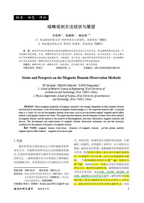
综述·动态·评论磁畴观测方法现状与展望许启明1,张振彬1,杨永明1,2(1. 西安建筑科技大学材料科学与工程学院,陕西西安 710055;2. 西安建筑科技大学理学院物理系,陕西西安 710055)摘 要:磁性材料的宏观磁性能主要是由磁畴结构及其运动变化方式所决定,因此磁畴图像的观测是一个很重要的研究课题。
目前,磁畴观测的方法已有很多种,如粉纹法、磁光效应法、电子全息法等。
本文主要介绍了各种磁畴观测方法的特点及发展状况,与铁磁学、电子信息、磁性材料及器件等学科的关系,指出磁畴观测方法的发展趋势,磁畴实验技术和装置的发展与完善将为磁畴动力学研究提供基础。
关键词:磁畴观测方法;磁畴动力学;粉纹图法;克尔磁光效应;磁力显微镜中图分类号:O482.5 文献标识码:A 文章编号:1001-3830(2010)04-0001-04Status and Prospects on the Magnetic Domain Observation MethodsXU Qi-ming1, ZHANG Zhen-bin1, YANG Yong-ming1,21. School of Material Science & Engineering, Xi'an University ofArchitecture and Technology, Xi'an 710055, China;2. Physics Department, School of Science, Xi'an University of Architectureand Technology, Xi'an 710055, ChinaAbstract: Macro-magnetic properties of magnetic materials were strongly dependent on their magnetic domain structure and its movement, so the observation of magnetic domain images is a very important research topic. At present, there is a variety of ways for the magnetic domain observation, such as powder pattern method, magneto-optical effect method, e-holographic method and others. This paper describes features and development of these observation methods of magnetic domain, and the relation to the research of ferromagnetism, electronic information, magnetic materials and devices. The development and improvement of magnetic domain observation techniques can provide necessary conditions for the research of dynamics of magnetic domain.Key words: magnetic domain observation; dynamics of magnetic domain; powder pattern method;magneto-optical effect method; magnetic force microscope1 引言磁性材料的宏观性能决定于材料磁畴结构和变化方式,对磁畴结构和变化方式的观测是铁磁学、信息科学和磁性材料与器件等学科领域的基础性研究之一。
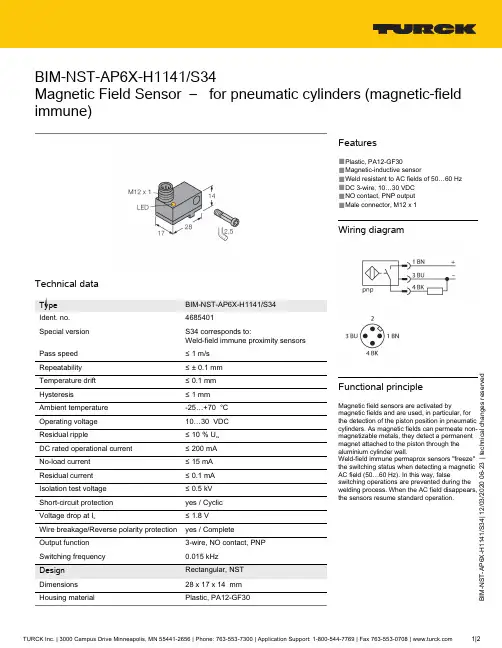
B I M -N S T -A P 6X -H 1141/S 34 | 12/03/2020 06-23 | t e c h n i c a l c h a n g e s r e s e r v e dBIM-NST-AP6X-H1141/S34Magnetic Field Sensor – for pneumatic cylinders (magnetic-fieldimmune)Technical dataBIM-NST-AP6X-H1141/S344685401S34 corresponds to:Weld-field immune proximity sensors≤ 1 m/s ≤ ± 0.1 mm ≤ 0.1 mm ≤ 1 mm -25…+70 °C 10…30 VDC ≤ 10 % U ss DC rated operational current ≤ 200 mA ≤ 15 mA ≤ 0.1 mA ≤ 0.5 kV yes / Cyclic ≤ 1.8 V Wire breakage/Reverse polarity protection yes / Complete3-wire, NO contact, PNP 0.015 kHz Rectangular, NST 28 x 17 x 14 mm Plastic, PA12-GF30Features■Plastic, PA12-GF30■Magnetic-inductive sensor■Weld resistant to AC fields of 50…60 Hz ■DC 3-wire, 10…30 VDC ■NO contact, PNP output ■Male connector, M12 x 1Wiring diagramFunctional principleMagnetic field sensors are activated bymagnetic fields and are used, in particular, for the detection of the piston position in pneumatic cylinders. As magnetic fields can permeate non-magnetizable metals, they detect a permanent magnet attached to the piston through the aluminium cylinder wall.Weld-field immune permaprox sensors "freeze"the switching status when detecting a magnetic AC field (50…60 Hz). In this way, falseswitching operations are prevented during the welding process. When the AC field disappears,the sensors resume standard operation.B I M -N S T -A P 6X -H 1141/S 34 | 12/03/2020 06-23 | t e c h n i c a l c h a n g e s r e s e r v e dTechnical dataAccessoriesKLN36970504Mounting bracket for mounting magnetic field sensors on dovetail groove cylinders or N T-groove cylinders; clamping width: 5.2…13.5 mm; material: Anodized aluminumKLN-SMC6970503Mounting bracket for mounting magnetic field sensors on SMC cylinders; clamping width 4 mm;material: Anodized aluminumKLF16970401Mounting bracket for mounting magnetic field sensors on profilecylinders with external dovetail guide;for all cylinder diameters, material:Anodized aluminumKLF26970402Mounting bracket for mounting magnetic field sensors on profile cylinders (IMI Norgren); cylinder diameter: 32…100 mm; material:Anodized aluminumSMC-325A3106Mounting bracket for mounting magnetic field sensors on SMC cylinders; clamping width 4 mm;material: Anodized aluminum。
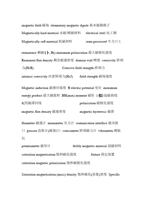
magnetic field 磁场elementary magnetic dipole 基本磁偶极子Magnetically hard material 永磁/硬磁材料electrical steel 电工钢Magnetically soft material 软磁材料semi-processed 半力口工remanence 剩磁(卜.Br) maximum polarization 最大磁极化强度Remanent flux density 剩余磁通密度domain wall 畴壁coercivity 矫顽力(HcB) Coercive field strength-矫顽力intrinsic coercivity 内禀矫顽力(HcJ) field strength 磁场强度Magnetic induction 磁感应强度B electric potential 电位maximum energy product 最大磁能积BH(max) moment 磁矩1但)退磁曲线8(用磁滞回线polarisation磁极化强度magnetic flux density 磁通密度magnetic hysteresis 磁滞fluxmeter 磁通计manometer 压力计comunication interface 通讯接口gausser高斯计(磁强计)coercimeter矫顽磁力计vibrometer测振仪permeameter 磁导计feebly magnetic material 弱磁材料saturation magnetization饱和磁化强度fixture 固定装置saturation magnetic polarization 饱和磁极化强度Saturation magnetization (mass) density 饱和磁化(质量)密度Specificsaturation magnetization 比饱和磁化强度Magnetic dipole moment 磁偶极矩incremental loop 增量回线gnetic moment 磁矩magnetic potential 磁位eddy current loss 涡流损耗curve 曲线100P 回线commutation curve 换向曲线Magnetic anisotropy 磁各向异性magnetic texture 磁织构Induced magnetic anisotropy 感生磁各向异性Magnetic anisotropic substance 磁各向异性物质Grain-oriented material晶体取向材料drill钻头fuse保险丝Thermally neutralized state 热致磁中性状态virgin state 初始状态Technical Specification 技术协议Drift 漂移NIM National Institute of Metrology 中国计量科学研究院IEC International Electrotechnical Comission 国际电工技术委员会DIN Deutsch Industrial Norman 德国标准German Institute of Standardization GB 国标ASTM 标准:American Society for Testing Material 美国试验材料学会QMS: Quality Management System 质量管理系统housing 测量主机temperature pole caps 高温极头thermocouple 热电偶Thermal element 热敏原件surrounding coils 环绕线圈integrated heating elements 集成力□热元件Room Temperature measurement 常温测量Pole Measuring 极头测量Segment pole coils 瓦型极头线圈Internal calibration 内部校准field coil场线圈pole coil极头线圈(arc) segment 瓦形square shape 方形Cubic 立方体Cylindrical圆柱体cylinder n.汽缸;圆柱状物ellipsoid椭圆体ring measuring cable 环行测量线Reference Samples 标准样品Ferrite Reference Sample 铁氧体标准样品Measuring range 测量范围NdFeB Reference Sample铉铁硼标准样品Resolution分辨率Shrink fitting 冷缩配合/烧嵌radial compression 径向压缩Nickel Reference Sample 银标准样品Permanent Magnet 永磁体3D-Helmholtz Coil三维亥姆霍兹线圈Electro magnet 电磁铁changeable pole cap 可更换极头voltage generator 电压发生器voltage integrator 电压积分器voltage indicator 电压指示器Measuring desk with Container 测量桌带货柜Integrator with very low drift with 24 bit A/D-converter积分器低漂移带24bit A/D转换器Windows-program多窗口界面Input resistance 输入电阻Interfaces 接口Connectors:Thermovoltage miniconnectors 连接器:热电压微型连接器data bank数据库printer打印机curves测量曲线data storage in an EXCEL-compatible 数据存储Excel 兼容Heating module 力口热模块Pole cap diameter 极头直径Inner diameter 内径temperature poles 温度极头thermovoltage mini socket 热电压微型插座Homogeneous Dia 平均直径Pole Face Dia 极面直径with feeder clamp connection 与馈线夹连接Incl. BROCKHAUS-Certificate 带Brockhaus 计量证书Allocation of filenames 分配文件名称depending on air-gap and pole cap 取决于空气间隙与极头Electrical drawings 电气图Mechanical drawings 机械图Drawings of part lists 零部件图Hardware set up 硬件调试LDR abbr.光敏电阻(light dependentresistor) PLM 脉冲宽度调制(Pulse-Length Modulation) PWM abbr.脉冲宽度调制(Pulse-Width Modulation) carbon fiber碳化纤维,碳素纤维optical fiber光纤,光导纤维steel fiber钢纤维;金属纤维fiber laser纤维激光器AlNiCo铝银钻ferrite铁氧体SmCo钐Shan钻磁铁NdFeB 铉铁硼slitting 分条single notching 单冲槽Steel plate shearer 剪板机interlocking with orientation 定向铆接Design and manufacture of carbide dies硬质合金模具的设计和制造Annealing and steam bluing 退火和发蓝core welding 铁芯焊接Plastic overmoulding 注塑rotor die casting 转子压铸Shaft insertion with liquid nitrogen 液态氮轴压入ventilation 通风设备Shaft production and assembling 轴的生产和组装aerospace 航空/天Axial轴向的radial辐射的multipolar多极的skewed偏斜的Amorphous alloy 非晶态合金cemented carbides硬质合金Austenitic stainless steel 奥氏体不锈钢solenoid 螺旋管Plasma cutting machine等离子切割机carbide stamping硬质合金冲压Blanking 落料notching 槽冲plastic overmoulding 注塑生产线Automatic press machine 自动压缩机high corrosion 高耐腐蚀性Low temperature coefficients 低温度系数scanner 扫描仪Parallelogram平行四边形diagonal对角线,斜的Generator stator and rotor parts 发电机定转子部件Pressure-riveting 压铆 laminations for automobile motor 汽车电机铁芯 EV Electron Volt 电子伏特 HEV Hybrid Electrical Vehicle 混合动力汽车Profilograph 轮廓曲线仪纵断面测绘仪表面光度仪Communication protocol (计算机)通讯协议 vacuum plate 真空板 Sucker 吸盘 torque force 扭力stamping 冲压 annealing 退火welding 焊接Actuator motor 执行器电机crane stator 起重机用电机定子Synergy 协同cocking-up 上翘Hydraulic pump 液压驱动 vibration free table 减震桌Electric cabinet 电控柜 barrier frequency 截至频率 Homogeneous primary windings 均匀的初级绕组Horizontal transmissibility 水平性传输resonance 协振 Elliptically rotation 椭圆旋转angular velocity 角速度 A real time acquisition system 实时采集系统phase control 相差 lead time 投产前准备阶段interlocking 咬合 gluing 粘合 Clamping 固定/夹紧burr 毛边/铁屑 anneal 退火/韧炼 Amortization 分期偿还 elongation 延展力 coax plug 共轴插头 Exciting current 励磁电流 software editor 软件编辑器 Hydraulic cylinder 液压缸log files 记录文件/日志文件Unloading problems 卸货问题trolly 货车/推车vacuum pumps 真空泵 Bending machine 折床 warranty guarantee 授权保证Meeting minutes 会议纪要 rectangular/sinusoidal wave 矩形波/正弦波 magnetizing current 励磁电流 amplitude stability 放大稳定性 The integral of the secondary voltage 次级电压的积分measuring gauge(n. 计量器;)测量仪 Function generator 信号发生器 Using Wattmeter-Ammeter-Voltmeter Method 用功率表/电流表/电压表 ARCNET interface-card ARCNET 网络接口卡等NO material 无取向试样 Magnetic displacement 磁位移 PO 是指采购订单生产计划是依据客户的采购订单(客户PO ) Ambit 范围/周围gauge 测量器 mechanical lifters 机械升起装置 connection screws 螺钉连接 solenoidn.[电]螺线管;螺线形电导管control loop 控制回路 Higher Harmonics 高次谐波Higher centrifugal force 高离心力Ceramic 陶瓷的Load cell 称重传感器/测力传感器G-clamp 螺旋夹钳 OD/ID(outside/inside diameter)外直径/内直径Sintered magnet 烧结磁铁slot ripple 线槽脉冲 thermal demagnetization 热退磁setup, commissioning (acceptance test)设定、命令(接收测试)operation of machine, Trouble shooting, calibration and adjustment and maintenance 机器操作、问题处理、校正与调试维护radium 半径 Magnetic moment 磁矩 helmholtz coil 亥姆霍兹线圈 DC Bias 直流偏磁 control algorithm 控制算法 strain gauge 变形测量器 sample clamp 样品夹。
石油英语词汇(M1)--------------------------------------------------------------------------------m 百万M 磁矩M 定倾中心M 分钟M 分子量m 毫m 胶结系数M 马赫M 麦克斯韦m 米M 摩尔m 泥浆M 平均M 其它M 千M 微M 阳的M 英里M 兆M 兆欧M 中m 重量摩尔浓度M 子午线M&FP 最大终压力M-ARY 多状态M-B 闭合-断开M-boundary 莫霍不连续面m-dichlorobenzene 间二氯苯m-dicyanobenzene 间苯二腈m-dihydroxy-benzene 间苯二酚M-discontinuity 莫霍不连续面M-G 电动发电机M-N plot 岩性-孔隙度交会图m-pentadiene 间戊二烯m-phenylene diamine 间苯二胺m-phthalic acid 间苯二甲酸M-Q register 乘数-商寄存器m-sequence m序列M-tooth M形齿m-xylene 间二甲苯m. daN 10牛顿-米M.a.B.S. 罐底机械沉渣m.a.p 管汇空气压力M.A.R. 多功能相控阵雷达M.A.R. 汞弧整流器M.A.W.P. 最高允许工作压力m.b.r.t. 转盘面以下米数M.C.W. 已调连续波M.C.W. 已调载波M.E. 采矿工程M.E. 采矿工程师M.E. 电磁的M.E. 机械工程师M.E. 主机M.E. 主作用力M.E.P. 平均有效压力M.F. 精整磨轧M.F. 中频m.g.s. 米-克-秒制m.i.p. 方法改进程序m.i.p. 平均指示压力m.i.p. 最小冲击脉冲m.kgf 公斤力-米M.L. 机器语言M.L. 模线M.L. 平均水平M.L. 吻合线M.L. 中线M.O. 汇票m.o. 手控的m.p.s. 米秒m.p.s. 英里秒m.p.s. 兆周秒m.pt. 熔点M.S. 磁谱仪M.S. 磁同步的M.S. 机械设备检查M.S. 理科硕士M.S. 软钢M.S. 选矿M.S. 主控开关M.S. 最大应力M.Sc. thesis 理科硕士论文M.T.S. 米-吨-秒M.U.F. 最高可用频率M.V. 初速M.V. 中等电压m.y. 百万年m.y.a. 百万年前MA 磁放大器MA 公制度量协会mA 毫安MA 滑动平均MA 文学硕士Ma 钨ma 岩石骨架MA 已调波放大器maar 火山口湖Maas compass 玛斯测斜仪Maas survey instrument 玛斯测斜仪MAASP 套管环隙最大容许压力Maastrichtian 马斯特里赫特统MAC 多极阵列声波测井macadam aggregate 粗粒掺和料macadam effect 自胶结作用macadam 碎石路;碎石macaroni pipe 细管macaroni rig 小直径油管修井机macaroni string 小直径油管柱macaroni tubing string 小直径油管柱macaroni 小直径管maccaboy 一种雷达干扰寻觅器maccaluba 泥丘macedonite 云橄粗面岩maceral variety 显微组分变种maceral 显微组分macerater 浸渍者;纸浆制造机;切碎机maceration 渗浸Mach number 马赫数mach 机加工的mach 机器mach 机械mach 机械师Mach 马赫Machairodus 短剑虎属mache 马谢machinability 可切削性machinable hardness 可机加工硬度machinable 可切削的machine address 机器地址machine aided cognition 计算机辅助识别machine arithmetic 机器运算machine attendance 机器保养machine attention 机器保养machine available time 机器可用时间machine charges 机器维护消耗machine check interruption 计算机检查中断machine check 机器校验machine code 机器代码;指令表machine computation 机器计算machine cut 机械切削machine cycle 机器工作周期machine equation 机器方程machine error 机器错误machine finishing 机械精加工machine format 机器格式machine gun oil 机枪油machine hand 机械手machine hours 机器运转时间machine instruction code 机器指令码machine instruction 机器指令machine language program 机器语言程序machine language 机器语言machine manufacturing 机器制造machine operation 机器操作machine operator 机器操作员machine parts 机器零件machine program 机器程序machine reel 机器磁带盘machine set bit 机镶细粒金刚石钻头machine setting 机床安装machine shop 机工车间machine time 机械开动时间machine tongs 机动大钳machine tool 工具机machine train 机组machine translation 机器翻译machine unit 机组;运算装置machine variable 计算机变量machine washer 平垫圈machine welding 机械化焊接machine word 计算机字machine works 机械厂machine 机器machine-hour 台-小时machine-oriented language 面向计算机的语言machine-spoiled time 机器故障时间machined parts 已加工部件machined surface 加工面machinery and equipment 机器设备machinery bronze 机用青铜machinery noise 机械噪声machinery oil 机械油machinery 机械machines and tools 机具machinework 机加工;机械制品machining allowance 机械加工余量machining precision 加工精度machining 机械加工machinist 机工;机械师machinofacture 机械制造;机加工产品machmeter 马赫表macigno 复理石相mackintosh 防水胶布;胶布雨衣Maclaurin series 马克劳林级数Maclurites 马氏螺属MACP 最大允许套压macrinite 粗粒体macro accounting 宏观会计macro call 宏调用macro check 宏观检查macro definition 宏定义macro etch 宏观腐蚀macro facility 宏指令macro generator 宏功能生成程序macro instruction 宏指令macro irregularity 宏观不均质性macro qualitative analysis 常量定性分析macro subsurface model 宏观地层模型macro 巨大的;大量的;宏观的;宏指令macro- 大macro-crack 宏观裂缝macro-equilibrium theory 宏观平衡理论macro-forecast 宏观预测macro-model 宏观模式macro-modular computer 宏模组件计算机macro-rheology 宏观流变学macro-theory of distribution 宏观分配理论macro-tool 探测范围大的测井下井仪macroanalysis 宏观分析macroassembler 宏汇编程序macroaxis 长轴macroburrowed strata 巨潜穴地层macrocinematography 放大电影摄影macroclastic rock 粗屑岩macrocleavage 粗劈理macroclimate 大气候macroclimatology 大气候学macrocode 宏代码macrocoding 宏编码macroconcentration 常量浓度macroconstituent 常量成分macrocosm 宏观世界macrocrystalline 粗晶的;宏晶;粗晶质macrocycle 大旋回macrocyclic compound 大环化合物macrodcopic displacement efficiency 宏观驱替效率macrodiscontinuity 宏观非连续性macrodispersoid 粗粒分散胶体macrodome 长轴坡面macroeconomic equilibrium 宏观经济平衡macroeconomic policy 宏砚经济政策macroeconomics 宏观经济学macroeffect 宏观效应macroelement 常量元素;宏组件macroexamination 宏观考察macrofeature 宏观特征macrofluid 宏观流体macrofold 宏观褶皱macrofossil 大化石macrofracture fabric 大裂缝组构macrofracture 宏观裂缝macrofragmental coal 显组分煤macrogeneration 宏生成macrogeological cycle 地质大旋回macrogphysics 宏观物理学macrograin 粗粒macrograined 粗粒的macrograph 肉眼图;宏观图;原形图;肉眼检查macrography 宏观照相术;宏观检查macrohistorical cycle 宏观历史循环macroite 粗粒惰性体macrolibrary 宏程序库macrometeorology 宏观气象学macrometer 测距器macromethod 常量法;宏观法macromolecular chemistry 大分子化学macromolecular compound 大分子化合物macromolecular dispersion 大分子分散体系macromolecular fluid 大分子流体macromolecular network structure 大分子网状结构macromolecular 大分子的macromolecule 大分子macrooscillograph 常用示波器macroparameter 宏参数macrophanerophytes 乔木macrophotograph 宏观摄影相片macrophotography 放大照相macrophyte 大型植物macropinacoid 长轴面macropipeline 宏流水线macropipelining 宏流水线操作macroplankton 大型浮游生物macroplate 大板块Macropolygnathus 巨多颚牙形石属macropore 大孔隙macroporous 大孔隙的macroporphyritic 大斑晶的macroprocessor 宏处理程序macroprogram 宏程序macroreticular weak acid resin 大网状弱酸树脂macroreticular-type resin 大网状树脂macrosamlpe 常量试样macroscopic absorption cross section 宏观吸收截面macroscopic angle 宏观角macroscopic anisotropy 宏观各向异性macroscopic boundary condition 宏观边界条件macroscopic capture cross section 宏观俘获截面macroscopic description 宏观描述macroscopic field 宏观场macroscopic flow direction 宏观流向macroscopic flow velocity 宏观渗流速度macroscopic flux 宏观流量macroscopic frac 宏观裂缝macroscopic fracture 宏观裂缝macroscopic heterogeneity 宏观非均质性macroscopic homogeneity 宏观均质性macroscopic instability 宏观不稳定性macroscopic interface 宏观界面macroscopic noise 宏观噪声macroscopic observation 宏观观察macroscopic path 宏观通道macroscopic pore structure 宏观孔隙结构macroscopic property 宏观特性macroscopic seismic phenomenon 宏观地震现象macroscopic slowing down power 宏观慢化能力macroscopic state 宏观态macroscopic streamline 宏观流线macroscopic sweep efficiency 宏观波及效率macroscopic test 肉眼检查macroscopic thermal neutron absorption capture cross section 宏观热中子吸收俘获截面macroscopic velocity 宏观速度macroscopic viscosity 宏观粘度macroscopic void 大孔洞macroscopic wateroil interface 宏观油水界面macroscopic 宏观的macrosection 粗视剖面;磨片组织图;宏观金相试片macrosegregation 宏观偏析macroseism 强震macroseismic 强震的macroshrinkage 宏观缩孔macrospore 大孢子macrosporinite 大孢子体macrostate 宏观态macrostatistical approach 宏观统计法macrostrain 宏应变macrostress 宏应力macrostructure 宏观结构;大型构造macrosymbiont 大共生体macrotectonics 大地构造macrothermophytia 高温植物群落macrotidal range 大潮差Macrotorispora 大一头沉孢属macrovisual study 宏观研究macrovoid ratio 大孔隙比MACS 多元自控系统MACS 中高度通信卫星macula 斑点;太阳黑点;矿石的疵点maculae macula的复数maculation 玷污Maculatisporites 斑纹孢属maculose rock 斑结状岩Mad Hatter's disease 慢性汞中毒症MAD 材料分析资料MAD 乘积加MAD 多孔磁心;多孔器件MAD 多路存取装置MAD 制造装配图MADDAM 微型组件及数字微分分析机made ground 现代沉积made up of 由…组成made-to-order 定做的madeirite 钛辉苦橄斑岩Madigania 马地干水母属madistor 晶体磁控管MADRE 马丁自动数据处理设备madreporite 筛板MADT 微合金扩散晶体管madupite 透辉金云斑岩mae 平均绝对误差Maedleriella 瘤球轮藻属Maedlerisphaera 梅球轮藻属maenaite 富钙淡歪细晶岩Maentwrogian 门特罗格阶Maexisporites 细粒面大孢属mafelsic 镁铁硅质的mafic hornfels 镁铁质角岩mafic margin 镁铁质边缘mafic mineral 镁铁质矿物mafic 镁铁质的mafr ite 富闪霞斜岩mafurite 橄辉钾霞岩MAG block 镁块MAG 磁的MAG 磁电机MAG 磁控管MAG 磁铁MAG 磁铁矿MAG 最大可用增益mag. 磁性mag. 量值;大小mag. 镁mag. 氧化镁mag. 杂志magacycle 巨旋回magallanite 沥青砾石magamp 磁放大器magazine camera 自动卷片照相机magazine 杂志magenta 品红;洋红;红色苯胺染料maghemite 磁赤铁矿magic chuck 快换夹具magic eye 光调谐指示管magic guide bush 变径导套magic hand 机械手magic ink 万能笔magic line 调谐线magic T 混合三通接头magic 魔术;魔力;魔术的;有魔力的magicore 高频铁粉心magistoseismic area 极震区magma association 岩浆共生组合magma basalt 玻璃玄武岩magma consolidation 岩浆固结magma contamination 岩浆混染magma hydrothermalism 岩浆热液作用magma intrusion 岩浆侵入magma series 岩浆系列magma splitting 岩浆分异magma 岩浆;稠液magmacyclothem 岩浆旋回magmagranite 岩浆花岗岩magmametamorphism 岩浆变质作用magmata magma 的复数magmatic activity 岩浆活动magmatic affiliation 浆岩亲缘magmatic assimilation 岩浆同化magmatic autocatalysis 岩浆自催化作用magmatic breccia 岩浆角砾岩magmatic complex 岩浆杂岩magmatic corrosion 岩浆熔蚀magmatic cycle 岩浆旋回magmatic differentiation 岩浆分异magmatic digestion 岩浆同化magmatic ejecta 岩浆抛出物magmatic emanation 岩浆喷气magmatic eruption 岩浆喷溢magmatic exhalation 岩浆喷发magmatic explosion 岩浆爆发magmatic flow 岩浆流magmatic gas 岩浆气magmatic hearth 岩浆源magmatic hydrothermal replacement 岩浆热液交代magmatic hydrothermalism 岩浆热液作用magmatic inflow 岩浆流入magmatic injection 岩浆贯入magmatic intrusion 岩浆侵入magmatic pneumatolysis 岩浆气化作用magmatic reemplacement 岩浆再侵位magmatic residual phase 岩浆残余相magmatic resorption 岩浆熔蚀magmatic rock 岩浆岩magmatic segregation 岩浆分结作用magmatic stoping 岩浆顶蚀magmatic suite 岩浆岩套magmatic wedging 岩浆楔入magmatic withdrawal 岩浆沉淀magmation 岩浆活动magmatism 岩浆作用magmatite 岩浆岩magmatogenic 岩浆成因的magmeter 直读式频率计magnacard 磁穿孔卡装置magnacycle 巨旋回magnadur 铁钡永磁合金magnafacies 大相magnaflux examination 磁粉检验magnaflux 磁铁粉检查法;电磁探矿法;磁粉探伤机;磁通量;磁力探伤magnalite 绿玄武土magnalium 镁铝合金magnascope 放象镜magnatector 测卡点仪magnechuck 电磁卡盘magnelog 磁测井magner 无功功率magnescope =magnascopemagnesia cement 镁氧水泥magnesia 氧化镁magnesial 镁质的magnesian limestone 镁质石灰岩magnesian siderite 镁菱铁矿magnesian 镁质的magnesioriebeckite 镁钠闪石magnesite 菱镁矿magnesium acetate 醋酸镁magnesium alloy diving suit 镁合金潜水服magnesium anode protection 镁阳极防蚀magnesium chloride 氯化镁magnesium nitrate 硝酸镁magnesium nitrite 亚硝酸镁magnesium oxide 氧化镁magnesium subgroup 含镁水亚组magnesium sulphate 硫酸镁magnesium 镁magnesium-zine binode 镁锌双阳极magnesium-zirconium drill rod 镁锆钻杆magnestat 磁调节器magnesyn 磁自动同步机magnet charger 充磁机magnet coil 电磁铁线圈magnet contactor 磁开关magnet core 磁心magnet cradle 磁铁支座magnet insert 磁心棒magnet junk retriever 磁力碎屑打捞工具magnet pole 磁极magnet support 磁铁支座magnet 磁铁magnet-qing 磁侵magnet-valve 电磁阀magnetic activity 地磁活动性magnetic after effect 磁后效应magnetic aging 磁老化magnetic airborne surveys 航磁测量magnetic alignment 磁力校准magnetic alloy 磁性合金magnetic amplifier 磁放大器magnetic amplitude 磁化曲线振幅magnetic analysis 磁力分析法magnetic anisotropy 磁各向异性magnetic anomaly follow-up 磁异常检查magnetic anomaly offset 磁异常位移magnetic anomaly 磁异常magnetic antenna 磁性天线magnetic area moment 磁矩magnetic artifact 人工磁效应magnetic attitude control system 磁力姿态控制系统magnetic attraction 磁引力magnetic axis 磁轴magnetic azimuth 磁方位magnetic balance 磁秤magnetic basement 磁性基底magnetic bearing 磁方向角magnetic biasing 磁偏magnetic bit extractor 磁力钻头打捞器magnetic blow 磁偏吹magnetic brake 磁力制动器magnetic bubble memory 磁泡存储器magnetic bubble 磁泡magnetic calibrating device 磁标定装置magnetic capacity 磁化率magnetic card 磁性卡magnetic cell 磁元件magnetic character 磁性字符magnetic characteristics 磁性magnetic charging method 磁充电法magnetic chart 磁力图magnetic circuit 磁路magnetic cleaning 磁清洗magnetic clutch 电磁离合器magnetic collar locator 磁性定位接箍magnetic compass 磁罗盘magnetic conductance 磁导magnetic conductivity 导磁性magnetic contactor 磁接触器magnetic core matrix 磁心矩阵magnetic core memory 磁心存储器magnetic core storage 磁心存储器magnetic core 磁心magnetic core-orientation test 磁法岩心定向测定magnetic correction 磁力校正magnetic coupling 磁耦合magnetic crack detection 磁力裂缝检查magnetic creeping 磁滞magnetic current line source 磁流线源magnetic curve 磁化曲线magnetic damper 磁铁阻尼器magnetic damping 磁阻尼magnetic data 磁力资料magnetic declination 磁偏角magnetic deformation 磁性变形magnetic delay-line 磁延迟线magnetic density 磁场强度magnetic detector 磁性检波器magnetic deviation 磁差magnetic dial gauge 磁性指示表magnetic differential flow recorder 磁性压差流量记录仪magnetic dip 磁倾角magnetic dipole moment 磁偶极矩magnetic dipole 磁偶极子magnetic directional clinograph 磁针式测斜仪magnetic disc head 磁盘磁头magnetic disc storage 磁盘存储器magnetic disc 磁盘magnetic disk memory 磁盘存储器magnetic disk 磁盘magnetic dispersion 磁漏magnetic displacement 磁位移magnetic disturbance 磁干扰magnetic diurnal variation 磁周日变化magnetic domain 磁畴magnetic drag 磁引力magnetic drive 电磁离合器驱动magnetic drop-type survey 磁性投入式测斜仪magnetic drum memory 磁鼓存储器magnetic drum storage 磁鼓存储器magnetic drum 磁鼓magnetic effect 磁化magnetic element 地磁要素magnetic equator 地磁赤道magnetic exploration 磁力勘探magnetic field intensity 磁场强度magnetic field strength 磁场强度magnetic field 磁场magnetic figure 磁场图形magnetic fishing tool 磁力打捞工具magnetic flag 磁性记号magnetic flowmeter 磁性流量计magnetic fluid clutch 磁流体离合器magnetic fluid 磁性流体magnetic flux density 磁通密度magnetic flux leakage 磁漏magnetic flux line 磁通线magnetic flux test 磁力线检验magnetic flux 磁通magnetic force 磁力magnetic gap 磁隙magnetic gauge 磁性测微计magnetic gear 磁力离合器magnetic geophysical method 磁法勘探magnetic gradiometer 磁力梯度仪magnetic head materials 磁头材料magnetic head 磁头magnetic heading 磁航向magnetic high 磁力高magnetic hot spot 磁热点magnetic hysteresis loop 磁滞回线magnetic hysteresis loss 磁滞损耗magnetic hysteresis 磁滞magnetic inclination 磁倾斜magnetic induced polarization method 磁感应极化法magnetic induction density 磁感应强度magnetic induction flowmeter 磁感应式流量计magnetic induction loop 磁感线圈magnetic induction 磁感magnetic inductive capacity 导磁率magnetic inductivity 导磁率magnetic inertia 磁惯性magnetic ink 磁性墨水magnetic inspection 磁力探伤magnetic insulation 磁绝缘magnetic intensity 磁化强度magnetic interference 磁干扰magnetic IP 磁感应极化法magnetic iron 磁铁magnetic key 磁力继电器magnetic lag 磁滞magnetic latitude 地磁纬度magnetic leakage factor 漏磁系数magnetic leakage flux 漏磁通量magnetic leakage 磁漏magnetic levitation 磁悬浮magnetic line of force 磁力线magnetic line 磁力线magnetic linkage 磁通匝连数magnetic locator sub 磁性定位短节magnetic log 磁测井magnetic logging 磁法测井magnetic low 磁力低magnetic map 地磁图magnetic mark 磁性记号magnetic maximum 磁力高magnetic memory 磁存储器magnetic meridian 地磁子午线magnetic method 磁法magnetic mineral 磁性矿物magnetic minimum 磁力低magnetic moment 磁矩magnetic momentum 磁通量magnetic multishots 磁力多点测斜仪magnetic MWD data 磁力随钻测量数据magnetic needle 磁针magnetic neutral state 磁中性状态magnetic north 磁北magnetic operational amplifier 磁运算放大器magnetic orientation 磁定向magnetic particle brake 磁粉闸magnetic particle examination 磁粉检验magnetic particle inspection 磁粉检验magnetic path 磁路magnetic permeability 磁导率magnetic permeance 磁导magnetic perturbation 磁扰magnetic pickup 电磁式拾音器magnetic plated wire memory 磁镀线存储器magnetic polarity reversal 磁极反转magnetic polarity stratigraphic classification 磁极性地层划分magnetic polarity 磁极性magnetic polarization 磁极化magnetic pole 磁极magnetic potential 磁势magnetic profile 磁力剖面magnetic property 磁性magnetic prospecting 磁法勘探magnetic proximity logging tool 磁性邻近径向测井仪magnetic pull 磁引力magnetic quantum number 磁量子数magnetic reactance 磁抗magnetic recorder 磁录音机magnetic rectifier 磁整流器magnetic reluctance 磁阻magnetic reluctivity 磁阻率magnetic remanence 剩磁magnetic resistance 磁阻magnetic resolution 磁性分离magnetic resonance imaging logging 核磁共振成象测井magnetic resonance 磁共振magnetic retardation 磁滞magnetic retentivity 顽磁性magnetic return path 磁通量回路magnetic reversal 倒转磁化magnetic rotation 磁旋magnetic rubber 磁性橡胶magnetic saturation 磁性饱和magnetic scalar potential 磁标量位magnetic scanning 磁扫描magnetic scattering 磁散射magnetic screen 磁屏蔽magnetic separation 磁力分离magnetic separator 磁力分离器magnetic shield 磁屏蔽magnetic shift register 磁移位寄存器magnetic signature 磁异常特征magnetic single-shot tool 磁性单点测斜仪magnetic spin 磁偶自旋magnetic starter 磁力起动器magnetic stirring apparatus 磁力搅拌器magnetic storage drum 存储磁鼓magnetic storage 磁存储器magnetic store 磁存储器magnetic storm 磁暴magnetic stratigraphic chassification 磁性地层划分magnetic stratigraphy 地磁地层学magnetic stress 磁应力magnetic surface 磁鼓面;磁带面magnetic survey 地磁测量magnetic susceptibility 磁化率magnetic switch 磁开关magnetic tape buffer 磁带缓冲器magnetic tape cassette equipment 盒式磁带机magnetic tape cassette 盒式磁带magnetic tape formatter 磁带格式器magnetic tape handler 磁带机magnetic tape label 磁带标号magnetic tape memory 磁带存储器magnetic tape playback system 磁带回放系统magnetic tape reader 磁带机magnetic tape recorder 磁带记录仪magnetic tape storage 磁带存储器magnetic tape subsystem 磁带子系统magnetic tape unit 磁带机magnetic tape 磁带magnetic testing 磁力探伤magnetic theodolite 磁经纬仪magnetic thickness log 套管壁厚磁测井magnetic thickness tester 磁性测厚仪magnetic thin film memory 磁膜存储器magnetic torque 磁矩magnetic torsion balance 磁扭秤magnetic track 磁通magnetic value 磁值magnetic vertical component 地磁垂直分量magnetic vertical intensity 地磁垂直强度magnetic water 磁水magnetic well logging 磁测井magnetic yoke 磁轭magnetic 磁的;磁化的;有吸引力的;磁性物质magnetic-card unit 磁卡片机magnetic-drum computer 磁鼓计算机magnetic-drum reader 磁鼓读出器magnetic-field test 磁力探伤magnetic-film memory 磁膜存储器magnetic-film 磁膜magnetic-matrix switch 磁模开关magnetic-polarity sequence 磁极层序magnetic-pulse welding 磁力脉冲焊magnetic-pulse 磁脉冲magnetically focused 磁聚焦的magnetically quiet 磁平静magnetically saturated 磁饱和的magnetics 磁学;磁性元件magnetisablilty 磁化能力magnetisation 磁化magnetism 磁学;磁性;磁力magnetite 磁铁矿;四氧化三铁锈层magnetite-rich rock 富磁铁岩magnetizability =magnetisabilitymagnetization characteristic 磁化特性magnetization current 磁化电流magnetization distribution 磁化分布magnetization error 磁化误差magnetization mapping 磁化制图magnetization =magnetisationmagnetize 磁化magnetized area 磁化区域magnetized bit 磁化位magnetized drilling assembly 磁化钻具magnetized layer 磁化层magnetized spot 磁化点magnetized water 磁化水magnetizer 感磁物;磁化器;导磁体magnetizing apparatus 磁化器magnetizing current 磁化电流magnetizing field 磁化场magnetizing force 磁化力magnetizing 充磁magneto detector 磁力检波器magneto field scope 磁场示波器magneto gyrocompass 磁力回转罗盘magneto 磁电机;磁的magneto- 磁力magneto-dipole 磁偶极子magneto-electric induction 磁电感应magneto-electric 磁电的magneto-electrotelluric exploration 大地电磁勘探magneto-electrotelluric 大地电磁的magneto-ionic theory 磁离子理论magneto-turbulence 磁性湍流magnetobiology 磁生物学magnetochemistry 磁化学magnetoconductivity 导磁率magnetodiode 磁敏二极管magnetoelasticity 磁致弹性magnetoelectric effect 磁电效应magnetoelectricity 磁电;电磁学magnetoemission 磁致发射magnetoflex 铜镍铁永磁合金magnetogasdynamics 磁性气体动力学magnetogram 磁强记录图magnetograph 磁强记录仪magnetogyric ratio 磁旋比magnetohydrodynamics 磁流体动力学magnetometer sensor 磁强仪传感器magnetometer survey 磁法勘探magnetometer 磁力仪magnetometric induced-polarization method 磁感应极化法magnetometric resistivity method 磁阻率法magnetometric 磁力的magnetometry 磁力测定magnetomotive force 磁通势magnetomotive 磁力作用的magneton 磁子magnetooptics 磁光学magnetophone 磁电话筒;磁带录音机magnetoplasmodynamics 磁等离子动力学magnetoresistance 磁阻magnetoresistivity 磁致电阻率magnetoresistor 磁控电阻magnetoscope 验磁器magnetosheath 磁鞘magnetosphere 磁性层magnetospheric substorm 磁层亚暴magnetospheric 磁性层的magnetostatic well-tracking 静磁井迹跟踪magnetostatics 静磁学magnetostratigraphic classification 磁性地层划分magnetostratigraphic unit 地磁地层单位magnetostratigraphy 磁性地层学magnetostriction transducer 磁致伸缩换能器magnetostriction vibrator 磁致伸缩振动器magnetostriction 磁致伸缩magnetostrictive drill 磁致伸缩钻具magnetostrictive transducer 磁致伸缩换能器magnetostrictive 磁致伸缩的magnetostrictor 磁致伸缩体magnetotail 磁尾magnetotelluric noise 大地电磁噪声magnetotelluric 大地电磁的magnetotellurics 大地电磁学magnetrol 磁放大器magnetron 磁控管magnettor 二次谐波型磁性调节器magni- 大magni-scale 放大比例尺magnification coefficient 放大系数magnification constant 放大常数magnification factor 放大系数magnification ratio 伸缩比magnification 放大magnified diagonal 交叉扩大法magnifier for reading 读数放大镜magnifier 放大器Magnifloc 聚丙烯酰胺型絮凝剂magnify 放大magnifying chart reader 卡片放大阅读器magnifying glass 放大镜magnifying power 放大率Magnilaterella 大侧牙形石属magniphyric 微粗斑状magnistor 磁变管magnitude of earthquake 地震震级magnitude of inclination 倾斜幅度magnitude portion 尾数部分magnitude 量度magnitude-intensity correlation 震级-烈度对应关系Magno 镍锰合金magno-ferrite 镁铁尖晶石Magnolipollis 木兰粉属magnon 磁子magnophorite 含钛钾钠透闪石magnophyric 粗斑状Magnuminium 镁基合金MAGS 气体保护金属极电弧焊magslip 无触点式自动同步机;旋转变压器;无触点自整角机mahogany acid 磺酸mahogany sulfonate 石油磺酸盐maiden field 未开发油、气田maiden voyage 初航maiden 新的;初次的mail order 通信订购mail transfer 邮汇mail 邮件;邮寄Maillechort 麦雷乔铜镍合金mailorder business 邮购业务main account 主要帐户main air blower 主风机main axis 主轴线main base 控制点main beam 主束main bearing 主轴承main block valve 总闸门main book 主要帐簿main bottom 基底;基座main budget 总预算main buoy 主浮筒main cable 大线main coil pair 主线圈对main construction 重点建设;重点项目;主体工程main control console 主控制台main control equipment 主控设备main control head 井口总闸门main coordinate 主坐标main current 主流main cycle 主旋回main deck 主甲板main diagonal 主对角线main dip 真倾角main drain 排水总管main drilling packer 主封隔器main drive gear 主齿轮main drive shaft 主动轴main fault 主断层main feeder 总馈线main file 主文件main flow direction 主流向main gathering station 总集油站main geosynclinal stage 主地槽阶段main joint 主节理main layer 主力层main lead 电源线main line 干线main lobe 主瓣main mast 主桅main maximum 主峰main memory 主存储器main menu 主菜单main motor 主电动机main office 总公司main pack 生产筛管段周围的砾石充填main pay 主要生产层main peak 主峰main phase 主相;主要阶段main pile 主桩main pipeline 干线main platform 主平台main pole 主磁极main pontoon 主浮筒main post 船尾柱main producing horizon 主力生产层main productive zone 主力生产层main profile 主测线main program sequence 主程序序列main program 主程序main project 重点项目main reaction 主反应main river 主流main routine 主程序main screen 生产筛管main sea 开阔海main shaft bearing 主轴轴承main shaft 主轴main shelf 主大陆架main signal 主控信号main sill 钻台主基木main spring 主弹簧main stem 主河道main storage 主存储器main store 主存储器main stream 主流main supply 干线电源main sweep 主扫描main switch 总开关;电源开关main tank 主油舱;主罐main valve 主阀main vertical zone 主竖区main winch 主绞车MAIN 维修main 总的main-transformer 主变压器mainframe computer 主计算机mainframe memory 主体存储器mainframe network 主机网络mainframe 主机;主机柜mainland 大陆mainliner 干线电机车mainstay industry 支柱产业maintain angle 稳斜maintainability 可维护性maintainer 维护人员maintenance by contractor 外包维修maintenance center 维修基地maintenance cost 维修费用maintenance crew 维修队maintenance depot 修理厂maintenance electrician 维修电工maintenance free 不需维修maintenance gang 维修班maintenance in storage 库存器材维修maintenance instruction 维修规程maintenance job 维修工作maintenance lorry 维修车maintenance man 维修工maintenance manual 维修保养手册maintenance of mud 泥浆的维护maintenance of reservoir pressure 油层压力保持maintenance overhaul 日常维修maintenance price 维持价格maintenance schedule 维修计划maintenance supply 维修器材maintenance support diving 维修辅助潜水maintenance truck 维修车maintenance 保持MAIS 坑道开采法maize 玉米;玉米的颜色Maj. 主要的;较大的major axis 长轴major calorie 大卡major clock 主时钟major company 大公司major component 主成分major cycle 大循环;主循环major diameter 外径major equipment 主要设备major executives 高级主管人员major fault 主断层major field 大油气田major fold 主褶皱major folded zone 大褶皱带major fracture 主裂缝major framework 主要控制网major function 优函数major grid line 主格线major industry 主要工业major joint 主接口;主节点;主节理major lobe 主瓣Major Oil Company 国际大石油公司major overhaul 大修major phase 主相major principal stress 最大主应力major product moment 大积矩major program 主要计划major repair 大修major reservoir 主力油层major rig repair 钻机大修major river bed 主河床major semi-axis 长半轴major stress 主应力major terms 常用名词major thrust plane 主冲断面major total 总计;主要统计值major 较大的;主要的;主科;主修majorant 强函数majority interest 多数股权majority share holding 多数股权majority vote method 多数表决法majority 大多数majorizing sequence 优化序列make a port 入港make a pull 起钻make a trip 起下钻make a well 钻一口井make and break rotary 上卸扣旋转工具make contact 工作触点make dead 断开make down 拆卸make footage 钻进make harbour 入港make hole 钻井make location 定井位make odds even 拉平make of casing 已下套管长度make or buy decision 自制或外购决策make reference 访问;查找make room 退让make the gas 去气make the kelly down 将方钻杆钻完make the rounds 检查油井或机器make time 匆忙完成作业make up 补充make 制造;制订;构成;引起;使得;做make-and-break coupling 快卸接箍make-and-break test 上卸扣试验make-and-break 接与断make-before-break contact 先闭后开触点make-position 闭合位置make-shift equipment 代用设备make-up chuck 钻杆旋接夹盘make-up fluid 补充液make-up gas 补给气make-up gun 上紧-卸开螺纹装置make-up hydrogen compressor 新氢压缩机make-up isobutane 补充异丁烷make-up of string 钻具组合make-up process water 补给工艺用水make-up pump 供水泵make-up tank 补充罐;配料罐make-up tongs 接管子用大钳make-up torque 上紧力矩make-up valve 备用阀make-up water 添加水make-up wrench 上紧螺纹管钳maker 出票人makeshift 临时代用品makeup and breakout 上紧-卸开螺纹making a connection 接单根making hole 钻井making-up shop 装配车间making-up unit 装配组件Maklaya 马克莱氏NFDA3属mal- 不mala fide 恶意malachite 孔雀石malacon 变水锆石maladjustment 失调malakon 变水锆石malalignment 不对准;相对位偏;偏心率;轴线不对准malapropos 不适当的malaspina glacier 山麓冰川malaxation 揉malaxator 揉和机;捏土机Malaygnathus 马来亚牙形石属malchite 微闪长岩malconformation 不均衡性;畸形maldistribution 分布不匀male and female cross 阳螺纹-阴螺纹十字接头male and female joint 阳螺纹-阴螺纹接头male connector 插头;阳螺纹接头male coupling tap 公锥male fishing tap 打捞公锥male gauge 塞规male joint 阳螺纹接头male packing brass 外填料铜衬套male plug 插头male spline 外花键male stab 插头male surface 被包容面male thread 阳螺纹male 阳性的maleic acid 马来酸maleic anhydride value 马来酸酐值maleic anhydride 马来酸酐maleinoid 顺异构物maleness 雄性malfeasant 渎职malformation 畸形malfunction routine 故障查找程序malfunction 不正常工作malicious act 恶意行为malignite 暗霞正长岩mall 锤;槌malleability 展性malleabilization 锻化malleable failure 延展性损坏malleable iron 韧性铸铁malleable 韧性的;可锻的malleation 锤薄mallet 木锤Mallexinis 棒瘤切壁孢属malm rock 粘土砂岩Malm 麻姆统malm 泥灰岩;钙质砂土;含白垩粘土malobservation 观察误差malodorant 加臭剂maloperation 误操作malposition 位置不正malpractice 渎职maltene 软沥青maltha 软沥青malthacite 水铝英石malthaite 软沥青malthene 软沥青质malthenes 石油脂malthite 软沥青malthoid 油毛毡malting coal 无烟煤maltose 麦芽糖Malvacearumpollis 锦葵粉属MAM 磁异常图mamanite 杂卤石mamelon 圆丘mamilite 镁铁白榴金云火山岩mammal fossil 哺乳动物化石Mammoth event 马默思地磁反向事件mammoth pool 大油藏mammoth pump 大型泵mammoth 大型的man rack 管道工用平板篷车man-auto 手动-自动man-capstan 人力绞磨man-computer communication 人-机通信man-computer interaction 人机联作man-hour 人-时man-in-the-sea diving technique 海中入水潜水技术man-machine communication 人机通信man-machine conversation 人机对话man-machine input-output system 人机联用输入-输出系统man-machine interaction 人机联作man-machine interactive processing system 人机对话处理系统man-machine interface 人机接口man-made basin 人造船坞。
磁场屏蔽区域英语Magnetic Field Shielding Region.Magnetic field shielding is a crucial technology that plays a pivotal role in various applications ranging from electromagnetic compatibility (EMC) to medical diagnostics and scientific research. The need to isolate specific areas from external magnetic disturbances or to protect sensitive equipment from harmful magnetic fields gives rise to the concept of a magnetic field shielding region.The fundamental principle behind magnetic fieldshielding is the use of materials that exhibit highmagnetic permeability, allowing magnetic field lines topass through them easily. These materials, known asshielding materials, effectively redirect the magnetic flux, reducing its strength in the shielded region.Types of Magnetic Field Shielding.There are two primary types of magnetic field shielding: active and passive.Active Shielding: Involves the use of a controlled magnetic field to cancel out the unwanted external magnetic field. This is achieved by generating a secondary magnetic field that opposes the primary field, effectively canceling it out. Active shielding requires a power source and can be highly effective but can also be complex and expensive.Passive Shielding: Relies on the use of materials with high magnetic permeability to absorb and redirect the magnetic field lines. Passive shielding is generallysimpler and cheaper but may not provide the same level of shielding as active methods.Applications of Magnetic Field Shielding.1. Electromagnetic Compatibility (EMC): In electronic devices and systems, magnetic field shielding is essentialto ensure compatibility and prevent interference between different components. Shielding can minimizeelectromagnetic emissions, preventing them from affecting other devices and vice versa.2. Medical Diagnostics: Magnetic Resonance Imaging (MRI) scanners, for example, require a strong and homogeneous magnetic field. Shielding is crucial to isolate thescanner's magnetic field, preventing it from affecting nearby equipment or patients.3. Scientific Research: Laboratories studying quantum phenomena, superconductivity, or other magneticallysensitive experiments require shielded regions to protect their experiments from external magnetic disturbances.Design Considerations for Magnetic Field Shielding.When designing a magnetic field shielding region, several factors need to be considered:Shielding Material Selection: The choice of materialis crucial, as it determines the effectiveness of the shielding. Materials with high magnetic permeability, suchas certain types of steel or alloys, are preferred.Shielding Thickness: The thickness of the shielding material affects its ability to absorb and redirect magnetic field lines. Thicker shields generally provide better shielding but can also increase cost and weight.Shielding Geometry: The shape and size of theshielding structure are important. For example, acylindrical shield is more effective at shielding acircular region than a planar shield.Gaps and Imperfections: Gaps or imperfections in the shielding material can compromise its effectiveness. Great care should be taken during installation to minimize these.Challenges and Limitations of Magnetic Field Shielding.While magnetic field shielding is highly effective, it also faces some challenges and limitations:Cost: High-quality shielding materials can beexpensive, especially for large-scale applications.Weight: Thick shielding materials can add significant weight to the system.Thermal Considerations: Some shielding materials may heat up when exposed to strong magnetic fields, affecting their performance.Shielding Effectiveness: Even with the best materials and design, complete elimination of the magnetic field may not be achievable.Conclusion.Magnetic field shielding regions play a crucial role in various applications, providing a controlled environment free from external magnetic disturbances. The choice of shielding material, design considerations, and limitations need to be carefully balanced to achieve the desired level of shielding while minimizing cost and weight. With ongoing research and development, we can expect furtherimprovements in magnetic field shielding technology, opening up new possibilities in various fields.。
N d2Fe14B晶粒取向程度对磁畴运动及磁性的影响规律 Effects of Grain Orientation on the Motion of Magnetic Domains and the Magnetic Properties of Nd2Fe14B潘 晶(南昌航空工业学院,南昌,330034) Pan Jing(N anchang Inst itute of A er onautical T echnolog y,N anchang,330034,China)摘 要 本文采用Bitter粉纹法研究并讨论了N d2F e14B晶粒取向程度对磁化、反磁化过程中磁畴运动及对磁体磁性的影响。
研究结果表明,磁中性状态的N d2Fe14B晶粒的磁畴畴壁与磁体成型磁场方向的夹角 越大,则在充磁过程中越难以变成单畴,在退磁过程中越容易形成反磁化畴。
磁体中 ≠0°的晶粒较多时,会使磁体的M-H曲线方形度降低,剩余磁化强度、磁能积减小。
关键词 Bitter粉纹法 晶粒取向 磁畴 磁性ABSTRACT T he effects of gr ain or ientat ion on the mot ion o f magnetic domains and pro per ties of N d2Fe14 B magnet hav e been studied.T he domains hav e been observ ed w ith t he Bitter met ho d.T he r esults hav e show n that the lar g er the a ng le (betw een dom ain w alls in a N d2F e14B gr ain in mag netism-free state and the mag netic field used in for ming the magnet blank), the mor e difficult the tr ansfor matio n fr om do mains in-to sing le do main in the magnetizat ion pr ocess,and the easier t he fo rmat ion of mag netically r ev er se do mains in the demag netizatio n pro cess.L arg e numbers o f N d2F e14B g rains w it h ≠0°co uld decr ease the squar e deg r ee of M-H curv e,the residual magnetization in-tensity,and the ener gy pr oduct of the mag net.KEY WORDS Bitter method,grain orientation, magnetic domain,magnetic properties1 引 言N d2F e14B晶粒易磁化轴(C轴)与整个磁体成型磁场(t轴)的夹角为 。
核磁共振英语词汇英文回答:Nuclear magnetic resonance (NMR) is a powerfulanalytical tool that utilizes magnetic fields and radio waves to investigate the properties of atoms and molecules. It offers a non-destructive and versatile technique for characterizing materials at the atomic and molecular level. NMR has various applications across multiple scientific disciplines, including chemistry, physics, biology, and medicine.The basic principle of NMR involves the interaction between atomic nuclei with a magnetic field. Certain nuclei, such as 1H (proton), 13C, 15N, and 31P, possess anintrinsic magnetic moment due to their nuclear spin. When placed in a magnetic field, these nuclei align with or against the field, resulting in two distinct energy states. By applying radio waves to the sample at specific frequencies, it is possible to induce transitions betweenthese energy states.The absorption of radio waves by the nuclei leads to the resonance phenomenon, which forms the basis of NMR. The resonant frequency for a particular nucleus depends on its chemical environment, including the electron density and surrounding atoms. By analyzing the resonance frequencies and patterns, NMR provides detailed information about the structure, dynamics, and interactions of molecules.NMR spectroscopy is a widely used technique for identifying and quantifying different atoms and functional groups within molecules. It plays a crucial role in determining the molecular structure of organic and inorganic compounds, as well as studying chemical reactions and reaction mechanisms. NMR also finds applications in drug discovery and development, protein structure determination, and metabolomics.In medical imaging, NMR is employed as a non-invasive tool for obtaining detailed anatomical and functional information about the human body. Magnetic resonanceimaging (MRI) utilizes NMR techniques to create high-resolution images of organs, tissues, and blood vessels. MRI is particularly valuable for diagnosing and monitoring a wide range of medical conditions, including brain disorders, cardiovascular diseases, and musculoskeletal injuries.NMR also has applications in other fields, such as materials science, polymer characterization, and geological studies. It is a versatile technique that provides valuable insights into the structure, dynamics, and properties of various materials and systems.In summary, nuclear magnetic resonance (NMR) is a powerful analytical tool that offers a non-destructive and versatile approach for investigating the properties of atoms and molecules. Its applications span multiple scientific disciplines, including chemistry, physics, biology, and medicine, providing insights into molecular structure, dynamics, and interactions.中文回答:核磁共振(NMR)是一种强大的分析工具,利用磁场和射频波来研究原子和分子的性质。
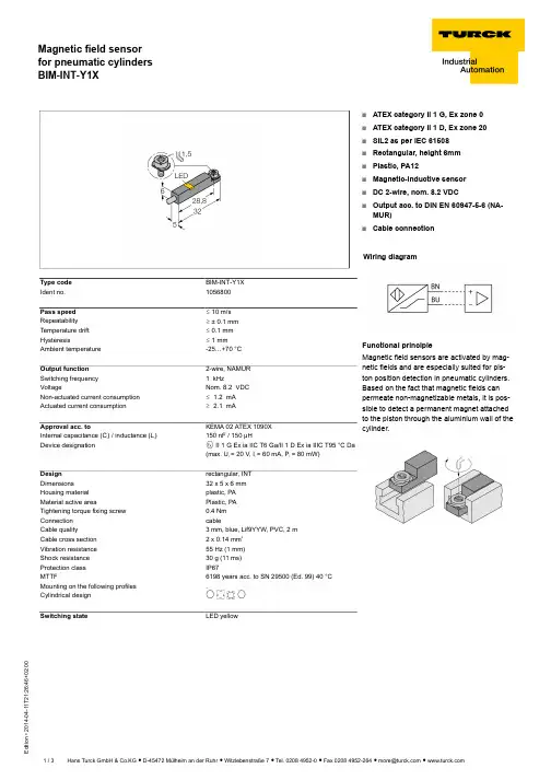
T 21:26:46+02:00Type code BIM-INT-Y1X Ident no.1056800Pass speed ð 10 m/s Repeatability ï ± 0.1 mm Temperature drift ð 0.1 mm Hysteresisð 1 mmAmbient temperature-25…+70 °C Output function 2-wire, NAMUR Switching frequency 1 kHzVoltageNom. 8.2 VDC Non-actuated current consumption ð 1.2 mA Actuated current consumptionï 2.1 mAApproval acc. toKEMA 02 ATEX 1090X Internal capacitance (C ) / inductance (L )150 nF / 150 µHDevice designationÉ II 1 G Ex ia IIC T6 Ga/II 1 D Ex ia IIIC T95 °C Da (max. U = 20 V, I = 60 mA, P = 80 mW)Design rectangular, INT Dimensions32 x 5 x 6 mm Housing material plastic, PA Material active areaPlastic, PA Tightening torque fixing screw 0.4 Nm Connection cableCable quality3 mm, blue, Lif9YYW, PVC, 2 mCable cross section2 x 0.14 mm Vibration resistance 55 Hz (1 mm)Shock resistance 30 g (11 ms)Protection class IP67MTTF6198 years acc. to SN 29500 (Ed. 99) 40 °C Mounting on the following profiles .Cylindrical design E N K F Switching stateLED yellows ATEX category II 1 G, Ex zone 0s ATEX category II 1 D, Ex zone 20s SIL2 as per IEC 61508s Rectangular, height 6mm s Plastic, PA12s Magnetic-inductive sensor s DC 2-wire, nom. 8.2 VDCsOutput acc. to DIN EN 60947-5-6 (NA-MUR)sCable connectionWiring diagramFunctional principleMagnetic field sensors are activated by mag-netic fields and are especially suited for pis-ton position detection in pneumatic cylinders.Based on the fact that magnetic fields can permeate non-magnetizable metals, it is pos-sible to detect a permanent magnet attached to the piston through the aluminium wall of thecylinder.T 21:26:46+02:00AccessoriesType codeIdent no.DescriptionDimension drawingIM1-22EX-R7541231Isolating switching amplifier, dual-channel; 2 relay outputs NO; input NAMUR signal; selectable ON/OFF mode for wire-break and short-circuit monitoring; adjustable signal flow (NO/ NC mode); removable terminal blocks; 18 mm width;universal voltage supply unitKLZ1-INT 6970410Accessories for mounting the BIM-UNT sensor on round cylinders; diameter: 32…40 mm; material: Aluminium; further mounting accessories for other cylinder diameters on requestKLDT-16913342Mounting on K dovetail groove cylinders; clamping width:10.5…12.4 mm; material: Aluminium; further mounting acces-sories for other clamping widths on requestKLR16970600Mounting on E round cylinders; material: Trogamid; please order retaining straps separatelyINT STOPPER 6900473Mounting on N T-groove cylinders; replacement without loss of switching point with additional clamp INT stopper; T-groove dimensions: 5…5.6 mmT 21:26:46+02:00Operating manual Intended useThis device fulfills the directive 94/9/EC and is suited for use in explosion hazardous areas according to EN60079-0:2012, -11:2012, -26:2007.Further it is suited for use in safety-related systems, including SIL2 as per IEC 61508.In order to ensure correct operation to the intended purpose it is required to observe the national regulations and directives.For use in explosion hazardous areas conform to classificationII 1 G and II 1 D (Group II, Category 1 G, electrical equipment for gaseous atmospheres and category 1 D, electrical equipment for dust atmo-spheres).Marking (see device or technical data sheet)É II 1 G und Ex ia IIC T6 Ga acc. to EN60079-0 and -26 and É II 1 D Ex ia IIIC T95°C Da acc. to EN60079-0Local admissible ambient temperatureATEX category II 2 G electrical equipment -40…+70°C, category II 1 D -25…+70 °C. The corresponding temperature classes are provided in the ATEX type-examination certificate.Installation / CommissioningThese devices may only be installed, connected and operated by trained and qualified staff. Qualified staff must have knowledge of protection classes, directives and regulations concerning electrical equipment designed for use in explosion hazardous areas.Please verify that the classification and the marking on the device comply with the actual application conditions.This device is only suited for connection to approved Exi circuits compliant to EN60079-0 and -11. Please observe the maximum admissible electrical values.After connection to other circuits the sensor may no longer be used in Exi installations. When interconnected to (associated) electrical equip-ment, it is required to perform the "Proof of intrinsic safety" (EN60079-14).When employed in safety systems to IEC 51408 it is required to assess the failure probability (PFD) of the complete circuitry.Installation and mounting instructionsAvoid static charging of cables and plastic devices. Please only clean the device with a damp cloth. Do not install the device in a dust flow and avoid build-up of dust deposits on the device.If the devices and the cable could be subject to mechanical damage, they must be protected accordingly. They must also be shielded against strong electro-magnetic fields.The pin configuration and the electrical specifications can be taken from the device marking or the technical data sheet.service / maintenanceRepairs are not possible. The approval expires if the device is repaired or modified by a person other than the manufacturer. The most important data from the approval are listed.。
低强度工频磁场对脑片海马区sEPSC 发放特性的影响王金海1,2,杜正高1,郑羽1,2,孔莹1,洪辉1,邱倩1(1.天津工业大学电子与信息工程学院,天津300387;2.天津市医学电子诊疗技术工程中心,天津300387)摘要:为研究磁场对脑片海马区自发兴奋性突触后电流(sEPSC )的生物刺激作用,利用实际测量、数学建模和Comsol 软件对典型磁刺激装置进行建模与仿真,确定磁场暴露区的磁场强度和分布特性,并采用膜片钳实验对磁场刺激条件下大鼠离体脑片海马区sEPSC 进行了研究.结果表明:磁场强度从刺激器舌面处到脑片区衰减125倍左右,且磁场进入溶液后分布更加均匀;磁场强度越高,sEPSC 的幅值和频率越低,当磁场强度达到2mT 时,神经元sEPSC 的幅值、频率、半波长、上升时间和衰减时间显著下降,说明随磁场磁剂量增加,磁场抑制sEPSC 的发放.关键词:工频磁暴露;磁场强度;分布特性;脑片海马区;sEPSC ;发放特性中图分类号:Q689;TP391.9文献标志码:A文章编号:1671-024X(2015)04-0052-06Effects of low intensity power frequency magnetic field on payment feature ofhippocampal sEPSC in vitro brain slicesWANG Jin-hai 1,2,DU Zheng-gao 1,ZHENG Yu 1,2,KONG Ying 1,HONG Hui 1,QIU Qian 1(1.School of Electronics and Information Engineering ,Tianjin Polytechnic University ,Tianjin 300387,China ;2.Center of Tianjin Medical Electronic Engineering Technology ,Tianjin Polytechnic University ,Tianjin 300387,China )Abstract :In order to investigate the biological stimulation of the magnetic field on the hippocampal spontaneous ExcitatoryPostsynaptic Current (sEPSC )of the brain slices ,the actual measurement ,mathematical modeling and Comsol software simulation were used to model and simulate a typical magnetic stimulation device,the magnetic field in 鄄tensity and distribution characteristics of the exposed area were confirmed.And the hippocampal sEPSC in the vitro brain slices under the magnetic field was studied with the patch clamp experiment.The results showed that the magnetic field intensity decreases by 125times from the simulator to the brain slice ,and the magnetic field distributes uniformly in physiological solution.The higher the magnetic field dose ,the lower the amplitude and frequency of sEPSC.When the magnetic field intensity reaches 2mT ,the amplitude ,fequency ,half -wave width ,the rise time and decay time of neuron sEPSC decrease significantly.This results illustrated that with the increase of intensity of magnetic field ,the magnetic field suppresses the sEPSC release.Key words :exposure to power frequency magnetic ;magnetic field intensity ;distribution characteristics ;hippocampus invitro brain slices ;spontaneous Excitatory Postsynaptic Current (sEPSC );payment feature收稿日期:2015-04-15基金项目:国家自然科学基金资助项目(61201106);国家级大学生创新创业训练计划项目(201410058027)通信作者:王金海(1966—),男,博士,教授,研究方向为生物信息提取.E-mail :*******************.cn随着科学技术的高速发展和人民生活水平的迅速提高,电力的广泛应用不可避免地引起越来越严重的电磁污染.近年来,人们开始关心这些弥散于我们周围的电磁场会对生物体尤其是人类产生何种影响,对电磁场生物效应的研究得到了各国学者的广泛关注.有研究表明,利用工频磁场对人体的中枢神经系统进行暴露辐射,结果显示人体的学习和预测能力出现下降、反应迟钝等现象[1];且有报道显示,工频电磁场影响大鼠的空间记忆力[2]和小鸡的迂回学习能力[3].海马区是神经系统中主管学习和记忆的重要区域[4],例如空间记忆、工作记忆和联系记忆等,临床新生儿的双侧海马损伤会造成严重的学习记忆障碍[5];海马区还与一些神经疾病有关,报道显示其是阿尔兹海默病、癫痫等精神疾病主要的病变位置[6-7].也有报道显示,30mT 恒定磁场能够明显延长海马区神经细胞的平均存活时间,且平均存活时间是对照组的一倍以上[8].磁场作为一种物理因素,对运动的带电物质有洛伦兹力的作用.工频磁场刺激是否对细胞间的带电粒天津工业大学学报JOURNALOFTIANJINPOLYTECHNICUNIVERSITY第34卷第4期2015年8月Vol.34No.4August 2015DOI :10.3969/j.issn.1671-024x.2015.04.011第4期子有磁场导向移动作用,从而影响到海马区神经元sEPSC 的电生理学特性?另外,研究低强度工频磁场对海马区脑片影响的报道也很少见.基于此,本文提出一种精确计算工频磁场作用于脑片区的磁剂量及其分布特性的研究方案,分析从磁场源到脑片区的磁剂量和分布特性,并讨论在该剂量下工频磁场对大鼠海马区sEPSC 发放特性的影响,为揭示工频磁场在海马区的生物效应奠定一定的理论和实验基础.1磁场刺激器建模仿真sEPSC 发放特性是衡量大脑海马组织功能强弱的一个重要指标,sEPSC 的发放反映海马神经元功能是否正常.通过上文可知,工频磁场对中枢神经及海马区神经细胞具有较大的影响.因此,精确计算作用在脑片上的工频磁场磁剂量对sEPSC 的检测具有重要的意义.本节将从实际测量、数学建模及Comsol 仿真3个方面对脑片区磁场强度进行建模仿真,考察脑片区的磁场强度和分布特性,保证脑片放置在暴磁区的最佳刺激位置,并从微观上定量确定磁场特性,为后续采用膜片钳技术分析sEPSC 的发放特性奠定基础.1.1磁场实际测量本实验自制磁场刺激器,磁路示例及等效电路如图1所示.磁路由马蹄形硅钢铁芯载体、培养皿中溶液、铁芯和培养皿间的空气3段材料组成.培养皿玻璃介质相应参数与空气相似,且所占空间很小,基本不影响磁场分布.其具体尺度参数为:铁芯采用冷轧硅钢片,厚2cm ,宽4cm ;线圈由直径0.8mm 漆包铜线绕制,匝数为310匝,舌面积为8cm 2;培养皿为玻璃材质,外壁和底部厚度均为1mm ,培养皿中装有人工脑脊液(arificial cerebrospinal fluid ,ACSF )[9].具体材料参数如表1所示.自制圆形线圈外接50Hz 交流稳压电源,可产生0~100mT 交变磁场,通过改变线圈中电流大小,可以调节线圈产生的磁场强度.在实际应用工频磁场对脑片区进行磁场刺激时,首先需要通过PF-035型数字特斯拉计测得暴磁区即培养皿处的磁场强度,和实验所需磁场强度进行对比,然后通过调节线圈输入电流大小,得到实验所需磁场刺激强度.当线圈中输入电流分别为0.21、0.32和0.56A 时,测得中心暴露区的磁场大小为0.5、1和2mT ;且通过多点测量证实,在中心暴露区磁场分布基本均匀,满足实验要求.但是,在进行多组试验时,由于每组实验所需的磁场刺激强度是不相同的,通过不断对比磁场强度和调节线圈电流大小来得到所需磁场强度的方法不够严谨,既耗费人力又浪费大量时间.因此,本文尝试采用数学建模的方法,建立线圈电流强度与暴磁区磁场强度之间的关系式,通过确定输入电流的强度,使得暴磁区即培养皿处能够获得所需的磁场强度.1.2数学建模针对如图1所示的磁刺激器,假设磁性材料内磁感应强度是均匀的,其值等于平均半径处的磁感应强度.设磁路平均长度为L ,截面积为A ,磁导率为μ,若线圈为N 匝,有电流I ,则外加磁动势为V m .具体参数为:铁芯磁路长L 1=220mm 、铁芯和培养皿顶部空气磁路长L 2=8mm 、培养皿中溶液磁路长L 3=32mm ;培养皿、铁芯舌面积和空气截面积分别为A 1=7.52πmm 2、A 2=20×40mm 2、A 2.由于培养皿和铁芯之间的缝隙只有4mm 的距离,因此,铁芯中磁感线设定都通过培养皿,这里设定空气截面积和铁芯舌面积相同.根据磁路的计算原理,外加磁动势V m 为:V m =NI =t乙H 軖·d l 軆(1)磁性材料内的磁通为:椎=s乙B 軑·d S 軋=BA =μNIA L=V mL /μA(2)如果磁路由n 段组成,则:ni =1移椎iRm i=V m (3)式中:椎i 为第i 段的磁通;R m i 为第i 段的磁阻,磁阻计表1材料参数Tab.1Material parameters材料名电导率/(S ·m -1)介电常数/(F ·m -1)磁导率/(H ·m -1)空气1.0011铜线59980000.0011铁芯70000000.0012530人工脑脊液 1.79109[10]1玻璃培养皿1.0021图1实际工频磁路示例及其等效电路Fig.1Actual circuit and equivalent cicuit(a )磁路示例(b )等效电路V m =NI+-L 2+L 2′椎L 3L 1L 1A 1L 2L 3L 2′A 2NIL 1王金海,等:低强度工频磁场对脑片海马区sEPSC 发放特性的影响53——天津工业大学学报第34卷算如下:R =R 1+R 2+R 3(4)式中:R 1=L 1/u 1A 2;R 2=(L 2+L 2′)/u 2A 2;R 3=L 3/u 3A 1;L 1、L 2+L 2′、L 3分别为铁芯、空气间隙和培养皿溶液中的磁路长度;u 1、u 2和u 3分别为铁芯、空气、溶液中的磁导率;A 2和A 1分别为铁芯(空气)和溶液的截面积;R 1、R 2和R 3分别为铁芯、空气和溶液中的磁阻.由式(1)—(4)得培养皿中磁场强度(B )计算公式为:B =V m /(RA 1)(5)根据式(5)计算可知,当线圈中分别通入0.083、0.85和1.65A 的电流时,空气间隙中磁场强度为0.5、1和2mT.通过数学建模,可以很快获得实验所需的暴磁区磁场强度.但是,该数学模型是以模型中的几何中心线为磁路的,和实际磁路相差明显;模型中没有考虑溶液的浓度、离子密度、电导率等参数,建模得到的结果和实际测量有一定误差.另一方面,实际测量中,由于特斯拉计精确度和灵敏度的限制以及空间上具体测量的难度,磁场分布的均匀性很难测量,数学建模也很难精确地确定磁场分布的情况,而磁场对脑片的刺激是整个区域的刺激,对于磁场均匀性需做进一步研究.因此,本文采用Comsol 软件进行进一步建模分析.1.3Comsol 建模仿真Comsol Multiphysics 是一款强大的有限元法分析软件.研究者可以根据实际情况选择不同的仿真环境和变量值,在结果中可清晰地看到物理场的分布情况.本文所研究的离体脑片及细胞的磁场辐射剂量在几个mT 范围内,在磁场刺激的时间段内,溶液的温度热效应忽略不计.在磁场刺激的过程中,脑片存活的环境是人工脑脊液.人工脑脊液和空气的区别在于前者介质为弱导体,对作用到脑片上的磁剂量和分布会产生一定影响,因为其包含生理溶液等因素的干扰,增加了磁场计算的复杂性.Comsol 仿真中能够设置溶液电导率、磁导率和密度等实际参数,通过仿真计算得到与实际所需磁场应输入电流大小最接近的电流值,并且从仿真结果中可以看到磁场强度和磁场强弱分布特性.为精确定量作用于脑片上各点磁场的剂量值,对sEPSC 发放特性测量提供精确的磁场刺激环境,本文采用Comsol Multiphysics 中的AC/DC 模块仿真建模与计算求解.建模时,对磁场刺激器采取1×1的比例建模,设定培养皿中装入空气和ACSF 两种不同的材料,材料参数根据实际参数设置,仿真出空气间隙磁场强度的大小和分布特性以及该磁场强度进入溶液中的大小和分布特性,并最终针对孵育环境中脑片上磁场的定量精确分布特性展开研究.当线圈中电流大小分别为0.105、0.20和0.42A 时,经Comsol 仿真得到暴磁区磁场强度为0.5、1和2mT 的磁场分布状况,进而确定脑片区的磁场分布特性,结果如图2所示.图2脑片区磁场强度的分布图Fig.2Distribution of magnetic field intensity in brain area(b )培养皿中介质为人工脑脊液(a )培养皿中介质为空气0.5mT1mT2mT0.1250.1240.1230.1220.1210.1200.1190.1180.1170.1160.1150.1560.1600.1640.1580.1620.1250.1240.1230.1220.1210.1200.1190.1180.1170.1160.1150.1560.1600.1640.1580.1620.1250.1240.1230.1220.1210.1200.1190.1180.1170.1160.1150.1560.1600.1640.1580.1620.1250.1240.1230.1220.1210.1200.1190.1180.1170.1160.1150.1560.1600.1640.1580.1620.1250.1240.1230.1220.1210.1200.1190.1180.1170.1160.1150.1560.1600.1640.1580.1620.1250.1240.1230.1220.1210.1200.1190.1180.1170.1160.1150.1560.1600.1640.1580.1620.51mT 0.510.470.480.490.50 1.07mT 1.071.061.051.041.031.021.011.000.990.992.09mT 2.082.062.042.022.001.981.961.941.936.36×10-3mT 6.3×10-36.2×10-36.1×10-36.0×10-35.9×10-35.8×10-35.79×10-30.01mT 14×10-312.7×10-30.010.03mT 27.3×10-324.9×10-30.02弧长/m弧长/m弧长/m弧长/m弧长/m弧长/m弧长/m弧长/m弧长/m弧长/m弧长/m弧长/m54——第4期根据离体海马区膜片钳实验,选择溶液中间直径1cm圆形区为脑片区,由于实验所用的脑片厚度范围在350~500μm,考虑到溶液中磁场在此厚度内的强度或分布性相差很小,且小尺度模型在Comsol画网格时大大增加了自由度数量,增加求解过程和时间,所以本文采取截面形式进行分析.图上方0.5、1和2mT数值表示舌面处磁场强度大小.对比图2(a)和图2(b)可以看出,磁场在铁芯舌面处的磁场强度是脑片上磁场强度的125倍左右,且磁场在溶液中分布更加均匀.2脑片sEPSC发放特性的测量膜片钳技术是测量脑片或细胞电生理特性的主要方法,具有高精度高稳定性的特点.本文通过建模仿真得到实验所需的准确磁场刺激强度,在此磁场强度刺激下通过膜片钳技术记录脑片的sEPSC,分析磁场刺激对sEPSC发放特性的影响.2.1膜片钳实验本实验采用中国医学科学院所属放射医学研究所实验动物中心提供的SD(Sprague Dawley)大鼠[11],鼠龄18~25d,雄性.并根据文献[12]的方法配置ACSF、切片液和全细胞记录sEPSC电极内液.对大鼠进行断头取脑,置于0~4°C的ACSF中1~2min,取出后置于震动切片机上切成350μm厚的脑片.室温下,将脑片放入ACSF中,并通入95% O2+5% CO2混合气体,孵育45min[13].孵育后,在显微镜下选取活性较好的脑片进行磁场刺激.准备好磁刺激装置并设定磁刺激器暴磁区的磁场强度(0、0.5、1和2mT),将培育好的脑片放入培养皿中,并移到刺激器的暴磁区.实验中脑片分为4组,分别是对照组(0mT)和工频磁场刺激实验组(0.5、1和2mT),10片一组,每片脑片上取活性最好的4个神经细胞来做实验,每组实验磁场暴露20min.经过40d试验后,最终得到142个有sEPSC发放的神经元细胞,本文从中选取122个发放幅值较大的数据进行论述.在室温下(20~23°C),利用EPC10-USB膜片钳放大器(HEKA,德国)进行全细胞膜片钳记录,通过Pulse软件设定好实验参数、刺激波形及数据采集.采用Minianalysis软件和Origin8.0统计软件分析实验数据.数据经P/N漏减处理后,进行统计与分析,结果用Means±SD表示.差异显著性检验采用单因素方差(one-way ANOVE)分析,post-hoc检验采用Scheffe检验方法进行统计,*P<0.05,**P<0.01,***P<0.001为显著性的3个层次[14].2.2脑片sEPSC的发放特性分析在本文试验条件下,大鼠海马CA1区锥体神经元sEPSC经0、0.5、1和2mT磁场刺激下的波形如图3所示,其幅值和频率如图4所示.由图3和图4可知,在0.5、1、2mT磁场强度下分别刺激20min后,大鼠海马CA1区锥体神经元sEPSC 发放的幅值和频率均下降;且随磁场剂量增高,sEPSC 的幅值和频率降低.由数据分析可知,在0.5mT磁场刺激下,sEPSC的幅值与正常对照组相比下降2046.37 4000350030002500200015001000500幅值/pA0.512图4sEPSC的幅值和频率Fig.4Amplitude and frequeney of sEPSC54321频率/Hz0.5121pA1280ms(a)0mT(b)0.5mT(c)1mT(d)2mT图3不同磁场强度刺激后sEPSC的波形Fig.3Waveform of sEPSC by different magnetic field intensity stimulation磁场强度/mT磁场强度/mT(a)幅值(b)频率王金海,等:低强度工频磁场对脑片海马区sEPSC发放特性的影响55——天津工业大学学报第34卷pA ,降幅达到49.8%;而在1和2mT 磁场刺激下,降幅增至80.3%和98%,说明1和2mT 磁场刺激显著抑制sEPSC 发放的幅度.在频率发放方面,0.5、1和2mT 磁场刺激下,频率的降幅达到40%、67.3%和75.6%,同样说明工频磁场对海马区CA1区神经元sEPSC 的频率发放发挥抑制作用.根据单因素方差(one-way ANOVE )分析显示,磁场作用明显抑制sEPSC 的幅值和频率发放,并且均有显著性差异(F (3,471)=137.32,P <0.01;F (3,526)=7.03156,P <0.05).2mT 磁场作用下神经元sEPSC 的幅值明显低于对照组,通过post-hoc 检验表明,2mT 磁场刺激后,对sEPSC 幅值和频率的抑制程度尤为显著(F =73.52,P <0.001;F =5.85,P <0.05).说明磁场已经影响到神经元的活性,导致神经元细胞膜的电生理特性降低.图5所示为大鼠海马CA1区锥体神经元单个sEPSC 的半波宽、上升时间和衰减时间的发放特性.由图5可知,0.5、1、2mT 磁场作用20min 后,大鼠海马CA1区锥体神经元单个sEPSC 的半波宽、上升时间和衰减时间的发放特性相似.与对照组相比,0.5和1mT 磁场作用后,sEPSC 的半波宽分别上升了0.29和0.64ms ,上升时间分别上升了0.27和0.49ms ,衰减时间上升了0.4和1.0ms .单因素方差(one -way ANOVE )分析显示,0.5、1mT 磁场作用使sEPSC 的半波宽、上升时间和衰减时间显著性增加(F (2,468)=67.49,P <0.01;F (2,468)=20.51,P <0.01;F (2,468)=87.12,P <0.01).由此说明,磁场刺激延长了海马CA1区锥体神经元sEPSC 的发放周期,从而降低了其发放频率,说明磁场刺激对脑片sEPSC 的频率发放有抑制作用.当增加磁场刺激剂量至2mT 后,与对照组相比,sEPSC 的半波宽、上升时间和衰减时间分别下降了0.63、0.79和0.3ms ,降幅达到42.3%、50.3%和23.4%.post-hoc 检验表明,与对照组相比,2mT 磁场作用显著抑制了sEPSC 半波宽、上升时间和衰减时间的发放(F =13.19,P <0.001;F =6.71,P <0.001;F =25.31,P <0.001).在2mT 磁场刺激下,脑片上神经元活性下降,细胞膜上离子通道活性随之下降,细胞突触间离子交换能力下降,因此,sEPSC 的半波宽、上升时间和衰减时间显著下降,说明2mT 磁场刺激显著抑制了sEPSC 的半波宽、上升时间和衰减时间的发放.综上所述,工频磁场抑制海马区神经元sEPSC 的发放特性,且随磁场强度的增加,磁场对sEPSC 幅值和频率的抑制越来越强,随之抑制sEPSC 半波、上升时间和衰减时间特性.这可能是由于:磁场的洛仑兹力能够影响带电粒子的移动,因此,磁场能够影响细胞膜的离子通透性和膜两侧的电位,导致机体内细胞内外电位失衡,从而影响带电物质的转移过程,产生一些生物效应.另外,在一些生物学的系统里,反磁体分子以高度规则方式排列,并以平行的反磁体矢量连接发挥作用[15].低强度工频磁场产生的洛伦兹力使得突触间带电状态的谷氨酸和Ca 2+、Na +、K +等离子非正常移动,不能与突触后膜上相应受体结合,从而影响到sEPSC 的放电特性.本实验结果提示,低强度磁场的生物刺激作用与细胞突触膜离子通道特性及通道构形变化有关,但仍需进一步从分子生物学及细胞信号转导方面进行分子层面的理论和实验验证.3结束语为了研究磁场对脑片sEPSC 电生理特性的生物刺激作用,本文设计了适用于离体脑片实验的50Hz 、21衰减时间/m s0.5122.01.51.00.50.0上升时间/m s0.51221半波宽/m s0.512图5单个sEPSC 半波宽、上升时间和衰减时间的发放特性Fig.5Issuance characteristics of half-wave width,rise time and decay time of single sEPSC磁场强度/mT(b )上升时间磁场强度/mT(a )半波宽磁场强度/mT(c )衰减时间56——第4期0~100mT磁信号发生器,通过实际测量、理论公式计算及Comsol建模仿真,得到磁场刺激器暴磁区的磁场强度和分布,最终确定作用到脑片上的磁场强度大小及分布情况.在此基础上,采用全细胞膜片钳技术,针对大鼠海马CA1区的锥体神经元细胞,记录由工频磁场诱发的sEPSC幅值及发放频率,在细胞水平上研究工频磁场对兴奋性突触后电流传递的影响.以sEPSC 的幅值、频率、半波长、上升时间和衰减时间为指标,研究工频磁场抑制兴奋性突触传递的可能机制.结果表明:在0.5和1mT磁场刺激下,神经元sEPSC的频率和幅值均有大幅度的下降,半波长、上升时间和衰减时间均高于未经过磁场刺激的神经元,说明细胞的兴奋性传递频率明显降低;当磁场强度达到2mT时,神经元sEPSC的幅值、频率、半波长、上升时间和衰减时间显著下降.参考文献:[1]段冠民,杨立新,李敬录,等.工频电磁场对中枢神经系统影响的观察[J].中国水电医学,2002(3):132-133.[2]MAJID J,SEYED M F,ALI R P,et al.Acute exposure to a50Hz magnetic field impairs consolidation of spatial memory in rats[J].Neurobiology of Learning and Memory,2007,88(4):387-392.[3]CHE Yi,SUN Huaying,CUI Yonghua,et al.Effects of expo-sure to50Hz magnetic field of1mT on the performance of de-tour learning task by chicks[J].Brain Research Bulletin,2007,74(5):178-182.[4]BROADBENT N J,SQUIRE L R,CLARK R E.Spatial memory,recognition memory,and the hippocampus[J].Proceedings of the National Academy of Sciences of the United States of America,2004,101(40):14515-14520.[5]MCAULIFFE J J,MILES L,VORHEES C V.Adult neurologicalfunction following neonatal hypoxia-ischemia in a mouse model of the term neonate:Water maze performance is dependent on separable cognitive and motor components[J].Brain Res,2006,1118:208-221.[6]KERR J E,BECK S G,HANDA R J.Androgens selectivelymodulate C-fos messenger RNA induction in the rat hippocampus following novelty[J].Neuroscience,1996,74(2):757-766. [7]PATCHEV V K,SCHROEDER J,GOETZ F,et al.Neurotropicaction of androgens:Principles,mechanisms and novel targets [J].Exp Gerontol,2004,39(11/12):1651-1660.[8]李刚,程立君,林凌,等.30mT恒定磁场对神经细胞钠通道特性的影响[J].光电子·激光,2009,20(12):1695-1698.[9]WEDEMEYER Carolina,ZORRILLA Javier,MART魱N San,et al.Activation of presynaptic GABAB(1a,2)receptors in-hibits synaptic transmission at mammalian inhibitory choliner-gic olivocochlear-hair cell synapses[J].The Journal of Neuro-science,2013,33(39):15477-15487.[10]姚陈果,莫登斌,孙才新,等.细胞电参数对内外膜跨膜电位影响的仿真研究[J].中国生物医学工程学报,2007,26(5):739-745.[11]JADIDI M,FIROOZAADI S M,RASHIDY P A,et al.Acuteexposure to a50Hz magnetic field impairs consolidation of spatial memory in rats[J].Neurobiology of Learning and Memory,2007,88(4):387-392.[12]刘振伟,杨胜,张永祥,等.突触前a7烟碱受体对海马神经元兴奋性突触传递的调控[J].生理学报,2003,55(6):731-735.[13]李刚,李丹丹,李媛媛,等.不同强度工频磁场对皮层神经元瞬时外向钾离子通道的影响[J].生物化学与生物物理进展,2011,38(11):1036-1042.[14]张莹,李伯勤,董娟,等.工频磁场对胎鼠大脑皮质神经元影响[J].中国公共卫生,2008,24(4):503-504.[15]ROSEN A D.Effect of a125mT static magnetic field on thekinetics of voltage activated Na+channels in GH3cells[J].Bioeletromagnetics,2003,24(7):517-523.王金海,等:低强度工频磁场对脑片海马区sEPSC发放特性的影响57——。
ElectricityMagnetic fieldMagnetic Field of a Cylindrical CoilDETERMINE THE MAGNETIC FIELD GENERATED BY COILS OF VARIOUS LENGTHS.UE3030500 10/15 UDFig. 1: Measurement set-up.GENERAL PRINCIPLESThe Biot-Savart law describes the relationship between magnetic flux density B and electric current I through a conductor of any arbitrary geometry. The calculation involves adding the contributions of infinitesimally small sections of conductor to find the overall magnetic flux density. The overall field is then determined by integrat-ing over the geometry of the conductor. In some cases, e.g. for a long cylindrical coil, there is a simple analytical solution to this integration.According to the Biot-Savart law, an infinitesimally small sec-tion of conductor d s through which a current I is flowing, gen-erates the following magnetic flux density at the point r(1) ()03d d 4s r B r I rμ⨯=⋅⋅π. B : magnetic flux density70Vs410Am-μ=π⋅: permeability of free spaceInside the cylindrical coil, the magnetic flux density is alignedparallel to the axis of the cylinder and is given by the following expression:(2) 0NB I L=μ⋅⋅. N : number of windings, L : length of coilThis applies as long as the length of the coil is much greater than its radius. The magnetic flux density does not therefore depend on the diameter of the coil and is proportional to the density of the windings, i.e. the number of windings per unit length, and the current through the coil.The experiment involves using an axial teslameter to measure the magnetic flux density inside long coils for currents of up to 20 A. It demonstrates that the flux density does not depend on the coil diameter but is proportional to the current and the winding density. In order to prove the latter, a coil is provided which allows the windings to be moved closer together or farther apart, i.e. varying the number of windings per unit length.LIST OF EQUIPMENT1 Field Coil, 100 mm U12252 1000591 1 Field Coil, 120 mmU1225310005921 Coil with Variable Number of Turns per Unit Length U8496175 1000965 1 Stand for Cylindrical Coils U8496150 1000964 1 Teslameter U33110 1003313/41 DC Power Supply 1 – 32 V, 0 – 20 AU11827 1012857/8 1 Set of 15 Experiment Leads 2,5 mm 2U13801 1002841 1 Barrel Foot, 1000 gU13265 1002834 1 Stainless Steel Rod, 250 mm U15001 1002933 1 Universal Clamp U13255 1002830 1 Universal Jaw ClampU132611002833SET-UP AND PROCEDURENote:By way of example, the experiment is carried out with 100 mm field coil (diameter D = 10 cm). ∙ Set up the experiment as shown in Fig. 1.∙Connect the field coil (D = 10 cm) to the 0 – 20 A output on the rear of the DC power supply. Do not turn on the power supply yet.∙Position the magnetic field probe by setting up the stand in such a way that the axial Hall probe (Fig. 2) is precisely in the centre of the coil.Fig. 2: Top: Magnetfeldsonde, 1 tangential Hall probe (z-direction), 2 axial Hall probe (x-direction), 3 probe car-rier. Bottom: Measurement of axial magnetic fields.The axial Hall probe measures the component of magnetic induction B along the axis of the probe. If the field B points along the axis of the probe (Fig. 2 below), the value displayed will be positive, whereas if it points the other way the value shown will be negative. ∙Connect the magnetic field probe to the correspondingsockets of the teslameter (Fig. 3).Fig. 3: Controls for teslameter:1 Connecting socket for magnetic field probe2 Digital display3 Measurement range selector, 20 mT4 Measurement range selector, 200 mT5 Measurement mode switch, axial (B X ) and tangential (B Z )6 Zero adjustment knob for B X with LED indicator7 Zero adjustment knob for B Z with LED indicator8 Output socket for axial mode B X9 Earth (ground) socket10 Output socket for tangential mode B Z 11 On/off switch ∙Turn on the teslameter, select a measuring range of 20 mT and turn the measuring mode delector switch to axial (B X ).∙Calibrate the zero point by turning the zero point calibra-tion knob B X until the display shows 0 or the lowest value achievable.∙Turn on the DC power supply. Increase the current from 0 up to 20 A in steps of 1 A. For each of these steps, read off the magnetic flux density B X , entering this value into Table 1 along with the current I set for that measurement.Safety instruction:∙ For a set current 10 A < I ≤ 20 A, only allow the current toflow for a brief period. ∙ Replace the field coil (D = 10 cm) by the coil with variable turns per unit length (Fig. 4).∙Set the lengths of the coil to be L = 7, 12, 17, 22, 27 and 32 cm, with each symmetrical around the centre of the coil. Repeat the measurement procedure described above for each of these lengths and enter all the values into Table 2.LFig. 4: Coil with variable number of windings per unit length.Note:The coil can optionally be mounted by its ends from two 1000964 stands. This means that it does not need to be taken off its stand every time the length is adjusted and that the magnetic field sensor does not need to be repositioned either.SAMPLE MEASUREMENTTab. 1: Magnetic flux density B as a function of current I through a field coil of diameter D = 10 cm.Tab. 2: M agnetic flux density B as a function of current I for various lengths of coil L.EVALUATION∙Plot the measurements in Table 1 in a graph of B againstI (Fig. 5).This verifies that the magnetic flux density B is proportional to current I through the coil as predicted by equation (2).Note:A corresponding measurement using a coil of diameter 120 mm (D = 12 cm) can demonstrate that the magnetic flux den-sityB remains proportional to the current I through the coil regardless of the coil’s diameter.∙Plot the measurements from Table 2, incorporating the various lengths as a parameter, in a graph of B against I (Fig. 6).This verifies that the magnetic flux density B is proportional to current I through the coil as predicted by equation (2) for any length of coil.Due to the inverse proportionality of the magnetic flux density B to the coil length L, the gradient of the lines decreases as the length gets longer.∙Knowing the number of turns on the variable length coil isN = 30, calculate the winding turns per unit length N/L and enter the results into Table 3.∙Take the magnetic flux densities B when current I = 20 A for each of the N/L values calculated from Table 2 and enter them in the corresponding cells of Table 3.∙Plot the measurements from Table 3 in a graph of B against N/L (Fig. 7).∙The flux density is confirmed to be proportional to the turns per unit length as long as the length of the coil is more than three times its radius. The diameter of the coil with variable turns per unit length is D = 10 cm.3B Scientific GmbH, Rudorffweg 8, 21031 Hamburg, Germany, Tab. 3: Magnetic flux density B as a function of number ofwindings per unit length N /L when I = 20 A. Number of windings N = 30.I / A0246B / mTFig. 5: Magnetic flux density B as a function of current Ithrough a field coil of diameter D = 10 cm.I / AB / mT0246Fig. 6: Magnetic flux density B as a function of current I usingthe coil with a variable number of windings per unit length for various lengths of coil L .B / mTFig. 7: Magnetic flux density B as a function of number ofwindings per unit length N /L when I = 20 A.。
magnetic induction intensity的缩写
Magnetic induction intensity,简称B,是一种描述磁场强度的物理量。
在磁学中,B代表磁感应强度,是描述磁场在某一特定点上强弱程度的物理量。
B的单位是特斯拉(T),国际单位制中的基本单位。
B的定义是磁感应线密度与真空中的磁导率μ的比值,即B=F/IL。
其中,F是磁场对电流的作用力,IL是电流元在磁场中的长度。
这个定义说明,B的大小与磁场对电流的作用力和电流元在磁场中的长度有关。
在磁学中,B与磁场强度H的关系是B=μrH,其中μr 是相对磁导率。
这个公式表明,在相同的磁场强度下,磁导率越大的物质,其磁感应强度越大。
B的测量方法有很多种,包括霍尔效应法、磁阻效应法、磁通门法等。
这些方法都是基于B对某些物理量的影响来间接测量B的值。
B在磁学中有广泛的应用,如在电机、发电机、变压器等电气设备中,需要测量和控制B的值以确保设备的正常运行和安全性。
此外,在地质勘探、医学成像、环境保护等领域,B也有着重要的应用价值。
总之,Magnetic induction intensity的缩写是B,它是一种描述磁场强度的物理量,在磁学中有广泛的应用。
Distribution of magnetic domain pinning fields in GaMnAsferromagnetic filmsJungtaek Kim, D. Y. Shin, and Sanghoon Lee*Physics Department, Korea University, Seoul 136-701, KoreaX. Liu and J. K. FurdynaPhysics Department, University of Notre Dame, Notre Dame, Indiana 46556, USA Using the angular dependence of the planar Hall effect in GaMnAs ferromagnetic films, we were able to determine the distribution of magnetic domain pinning fields in this material. Interestingly, there is a major difference between the pinning field distribution in as-grown and in annealed films, the former showing a strikingly narrower distribution than the latter. This conspicuous difference can be attributed to the degree of non-uniformity of magnetic anisotropy in both types of films. This finding provides a better understanding of the magnetic domain landscape in GaMnAs that has been the subject of intense debate.PACS numbers: 75.50.Pp, 75.30.Gw, 75.40.Gb*Electronic address: slee3@korea.ac.krThe ferromagnetic semiconductor GaMnAs continues to be the subject of intense interest due to the opportunities which it may provide for spintronic applications [1-3]. Many of its physical properties, such as the effect of low temperature annealing on the Curie temperature [4-8], the role of Mn ions at interstitial positions [7, 9, 10], and the dependence of magnetic anisotropy on strain and on carrier density, have been extensively investigated [11-13].The fundamental question of the uniformity of magnetic phase in GaMnAs is, however, still under debate. For example, the ac susceptibility measurements of Hamaya et al. [14] of GaMnAs films have led these authors to suggest a mixed magnetic phase model of GaMnAs. Wang et al. [15], on the other hand, who also carried out ac susceptibility studies on GaMnAs films, interpret their data in terms of temperature-dependent changes in magnetic anisotropy by assuming a single uniform magnetic phase. It is thus clear that further studies are needed to resolve the fundamental issue of the magnetic domain landscape in GaMnAs.A major advance in this area has been made by Welp et al. [16], who used magneto-optical imaging to map the magnetic domain structure in GaMnAs. This study demonstrated a landscape comprised of multiple domains with different directions of magnetization coexisting during magnetization reversal. The magnetotransport measurements of Shin et al.[17] provided further evidence for the existence of stable multidomain structures which accompany the magnetization reversal process in GaMnAs.In this letter we report a study of the multidomain structure in GaMnAs during magnetization reversal carried out by an alternative approach of changing the direction of the applied magnetic field while its magnitude is kept constant. It will be shown that this approach provides direct information on the distribution of pinning fields for magnetic domains with different orientations of their local magnetization.A GaMnAs film with 6.2 % of Mn and a thickness of 100 nm was used in this study. Thedetails regarding growth, annealing, and sample preparation are described elsewhere [19]. Curie temperatures T C of 62 and 136 K were estimated for the as-grown and annealed films from the temperature dependences of their respective resistivities (see inset in Fig. 4). Hall measurements revealed the magnetic easy axes to lie in the layer plane in both samples. The magnetic anisotropy within the plane is, however, quite different in the two cases, as revealed by the angular dependence of the planar Hall effect (PHE). The dependence of PHE on the magnetic field orientation was measured as follows. The magnetization of the sample was first saturated by applying a field of 4000 Oe at a given angle. The field was then reduced to the desired strength, and the PHE was measured as the field direction was rotated without changing field strength . This was repeated for a series of field strengths. The azimuthal angle was measured counterclockwise from [110] crystallographic direction (i.e., from the direction of the current).Representative angular dependences of the planar Hall resistance (PHR) obtained for as-grown and annealed GaMnAs films at 13 K are shown in Fig. 1. The PHR is seen to vary between positive and negative values as the field is rotated, showing a hysteresis between clockwise (CW) and counterclockwise (CCW) rotations. This type of angular dependence of PHR has already been observed in GaMnAs films [19, 20], and can be described by the following expression [21]2PHR sin 2M k R M tϕ=, (1) where t is the film thickness, M ϕis the angle between the direction of the current and the magnetization M , and k is a constant related to the anisotropic magnetoresistance. Note that the behavior of PHR is strikingly different in the two samples, showing an abrupt transition between its maximum (2k M t + ) and minimum (2k M t− ) values in the as-grown film,and a smooth broad transition for the annealed film.In order to investigate the magnetic domain structure associated with the reorientation of magnetization during the rotation of the field, we have focused on the transition region indicated by the shaded area in Fig. 1. This region includes the crossing by the field direction of the [110] crystallographic axis. In this angular range the direction of magnetization changes between the [100] and [010] directions via domain nucleation and propagation, in a process similar to that discussed in Ref. [16]. The value of PHR in this region will therefore reflect the fractions of the sample area occupied by domains oriented along [100] and [010]. Note that magnetization in these directions corresponds to the minimum and maximum values of R PHR , respectively, when the entire sample is in single-domain state [17]. The fractional area p of magnetization along the [010] direction at any point during the transition from [100] to [010] (i.e., in the case of CCW rotation of the field) can be calculated from thesimple relation, max PHR PHR1/2(1/)p R R =−, given in Ref. [22]. The observed values of p are plotted in the left inset in Fig. 2.The direction of magnetization in an in-plane magnetized GaMnAs film is determined by the magnetic free energy, given by [23]22U C sin (/4)cos 2cos()M M M H E K K MH ϕϕϕϕ=+−−, (2) where H is the external magnetic field, U K and C K are uniaxial and cubic anisotropycoefficients, respectively, and M ϕ and H ϕ are angles of the magnetization and of the applied magnetic field measured from the [110] direction. The magnetic energy difference between magnetizations along [100] and [010] directions is then[010][100][010][100]2cos sin ()/2H M M E E E MH ϕϕϕ⎡⎤Δ=−=−⎣⎦, (3)where the orientation of magnetizations is given by the angles [100],[010]M ϕ. Note, however, thatthese orientations may be slightly mis-aligned with [100] and [010] due to the presence of the external magnetic field and to contributions from uniaxial anisotropy [18].Since the energy difference E Δ between the two directions of magnetization varies as cos H H ϕ in Eq. (3), it can be continuously swept by changing the direction of the appliedfield. This provides a very direct handle for investigating the pinning energy [24] distribution of magnetic domains, since only those areas having a domain pinning energy of the same or smaller magnitude than E Δ will make a transition from [100] to [010] during the scan of E Δ. As the sample breaks up into regions with two different directions of magnetization, the value of PHR will change to reflect the fractional areas corresponding to these two magnetization orientations. From the data shown in the left inset in Fig. 2 (p vs. H ϕ) and the relation given in Eq. (3) (E Δ vs. H ϕ), one can relate the fraction p to the value of /E M Δ, as shown in the right insets in Fig. 2. Note that the relation between p and /E M Δ is a measure of the field strength required to reorient the domain magnetization from the [100] to the [010] direction. The derivative of p with respect to /E M Δ then provides the probability of finding a domain with a pinning field /p H E M =Δ, which is the threshold external field required to cross the [110] direction. The probability distributions of domain pinning fields obtained in this way are plotted for both samples in Fig. 2. This probability can very nicely fit by a Gaussian distribution function given by2()()p H H f H ⎡⎤−= , (4) where p H is the pinning field for a domain with a given orientation,avg H is the averagepinning field over the entire ensemble of domains in the sample, and σ is the standard deviation of the pinning field fluctuation. The value of avg H obtained from the fits is37.70.43Oe ± for the as-grown and 8.60.30Oe ± for the annealed sample.It is most interesting that the domain pinning field distribution for the as-grown sample shown in Fig. 2 is confined to a very narrow region, indicating that domain pinning is quite homogeneous over the entire sample. Since the domains comprising the sample have nearly identical pinning fields, they rotate coherently during magnetization reversal. This behavior is consistent with the uniform magnetic phase model adopted by Wang et al. for the interpretation of their ac susceptibility data obtained on as-grown GaMnAs film.In contrast to the as-grown sample, domain pinning fields in the annealed sample are distributed over a broad region, as seen in Fig. 2. Note that there even is a finite probability p for a region of negative pinning fields, indicating that there exist areas in the film in which magnetization direction can change in the absence of an applied magnetic field. The phenomenon of negative pinning fields is usually observed in magnetic multilayer systems comprised of ferromagnetic and antiferromagnetic layers. In that case a strong coupling between adjacent magnetic layers provides a negative pinning field for the ferromagnetic layer [25]. Our sample, however, consists of a single ferromagnetic GaMnAs film, and it is difficult to identify a mechanism that would be analogous to that discussed in Ref. [25]. The negative pinning field in our case must therefore have an entirely different origin.To gain some insight into the broad distribution of pinning energies in annealed GaMnAs (including negative values), we must reexamine the distribution of magnetic anisotropy within the sample. In the analysis presented above we assume the entire film to be uniformly dominated by the same type of anisotropy (specifically, cubic). However, magnetic domains in a GaMnAs film can in principle have different magnetic anisotropies, resulting in different magnetization directions at zero magnetic field. It is now well established that magnetic anisotropy in GaMnAs is a sensitive function of the hole concentration [11, 13]. Small fluctuations of this parameter can thus produce regions with different magnetic anisotropy (i.e., different relative strengths of K U and K C). This in turn can result in local variations ofmagnetic energy profiles, leading to a broad distribution of magnetic pinning fields, as is observed. The observation of the negative pinning field can also be understood in terms of this picture. Assume, for example, that there are some areas dominated by uniaxial anisotropy along [110], and some dominated by cubic anisotropy along the <100> directions. The magnetization of each area will then have tended to align along the directions of magnetic energy minima determined by the anisotropy at zero field. As the magnetization makes the transition from [100] to [010] directions, its relaxation toward the [110] direction in uniaxial-anisotropy-dominated areas can then be viewed as a rotation of magnetization from [100] to [010] in a fraction of the sample. This will manifest itself as a negative pinning energy in the analysis used above, where the magnetization was assumed to make a transition from [100] to [010].To support the existence of areas dominated by different magnetic anisotropies in the annealed sample, we performed field scans of PHR with different directions of the applied field. Data presented in Fig. 3 show that the value of PHR changes significantly when the field is reduced toward zero even before its direction is reversed. This behavior is very different from what we observed in as-grown GaMnAs film with a strong cubic anisotropy, in which an abrupt change of PHR occurs only after the field direction is reversed [16,20]. Furthermore, in field scan experiments on annealed GaMnAs films the PHR value at zero field is neither a maximum nor a minimum, which can only occur when the magnetization points along one of the in-plane <100> directions over the entire sample in the form of single domain.Note also that PHR returns to the same value at zero field independent of what was the field direction during the scan. These observations directly suggest that the sample consists of some areas with strong uniaxial anisotropy along [110], and some with strong cubic anisotropy along the <100> directions. The magnetization of the sample at zero field is thengiven by the combination of magnetic domains with magnetizations along [110] (uniaxial-anisotropy-dominated areas) and along <100> (cubic-anisotropy-dominated areas), as shown in the right-hand inset in Fig. 3.In the above configuration involving domains with two different orientations, the direction of the average magnetization at zero field will lie between these two orientations, thus resulting in an intermediate value of PHR, exactly as observed in experiment. Furthermore, this distribution of magnetic domains is intrinsic to the film, and will thus result in the same value of PHR at zero field, regardless of the direction of the field applied during the scan. This is confirmed by the entire set of field angle data in the left-hand inset of Fig. 3, which clearly show that PHR changes only between two values (positive for [100] and [110] combination, and negative for [010] and [110] combination), both of the same magnitude. This observation directly indicates that the annealed GaMnAs film consists of areas having different magnetic anisotropies, similar to the mixed magnetic phase model suggested by Hamaya et al. [14].The pinning field distribution caused by magnetic fluctuations was further tested by investigating the process of magnetization reorientation for various field strengths, chosen so as to cover the distribution of pinning fields in the sample. If the pinning field distribution shown in Fig. 2 corresponds to a specific distribution of magnetic regions in the sample, only a fraction of the sample with domain pinning fields which are smaller than the applied external field will be able to respond to the field as it is rotated. This will be reflected in theϕ, since in the reorientation process only those amplitude of PHR as a function of the angleHareas which can follow the rotation of the field will contribute to changes of the PHR value. The field dependence of the amplitude of PHR normalized by the PHR maximum observed at 4000 Oe is shown Fig. 4. The normalized PHR amplitude remains constant (close to unity) at fields above 40 Oe, indicating that above 40 Oe practically the entire sample follows therotation of the field. This is consistent with the domain pinning field distribution shown in Fig. 2, where the upper ends of the distributions for both samples lie around 40 Oe. At lower fields, on the other hand, the amplitude of PHR is clearly seen to decrease as the field is reduced, since the areas having pinning fields larger than the strength of the applied field can no longer follow the rotation of the field. Thus the lower the field, the lesser fraction of the sample can respond to the field rotation. As seen in Fig. 4, in the as-grown sample the amplitude of PHR drops rapidly to zero within a very narrow field window, while the decrease of PHR in the annealed sample is much more gradual. This behavior directly reflects the difference of domain pinning field distributions in as-grown and annealed GaMnAs.Interestingly, the pinning field distribution shown in Fig. 2 for GaMnAs films also provides qualitative insight into the temperature dependence of the resistivity shown in the inset of Fig. 4. It is now well established that the peak in the temperature scan of the resistivity is an indication of the magnetic phase transition [6]. The resistance peak in annealed GaMnAs samples -- although it is shifted to a higher temperature, indicating an increase of the Curie temperature -- is systematically observed as a broad, rounded maximum as compared to the sharp peak seen in as-grown samples [4, 6, 8]. This has always been rather surprising, since annealing leads to an overall improvement of magnetic properties of GaMnAs films, such as an enhancement of T C and a reduction in the concentration of interstitial Mn ions [4-9]. However, one can see from Fig. 2 that the pinning field distribution in annealed GaMnAs is much broader than in as-grown material. This suggests that annealing leads to an increase of magnetic fluctuations (in agreement with Refs. [7] and [14]); and it is reasonable to expect that the more magnetic fluctuations in the film, the broader will be the temperature range needed to complete the magnetic phase transition of the entire film. The commonly observed difference in the resistivity peaks of as-grown and annealed GaMnAs can therefore be readily related to the difference in their magnetic pinning field distributions.In conclusion, we have investigated the domain pinning field distribution of ferromagnetic GaMnAs films by PHE measurements as a function of applied field orientation. While a narrow pinning field distribution was obtained for as-grown GaMnAs, annealed GaMnAs film exhibited a strikingly broad range of pinning fields. Such pinning field distribution was interpreted in terms of fluctuations of magnetic anisotropy over the area of the film. All domains comprising as-grown GaMnAs have similar magnetic anisotropy (predominantly cubic), resulting in a uniform behavior of the sample as a whole. In contrast, domains in annealed GaMnAs films have a broad range of pinning fields (including even a non-zero probability of negative pinning fields), indicating the existence of areas with various degrees of uniaxial anisotropy. This broad pinning field distribution agrees with the mixed magnetic phase model proposed in Ref. [14]. The present study therefore demonstrates that the magnetic nature of GaMnAs films can be represented either by a single (uniform) phase, or by a mixed phase model, depending on the degree of magnetic anisotropy variation related to spatial magnetic fluctuations within the film.This work was supported by the Korea Research Foundation Grant KRF-2004-005-C00068; by the Seoul R&DB Program; and by the National Science Foundation Grant DMR06-03762.[1] G. A. Prinz, Science 282, 1660 (1998).Wolf et al., Science 294, 1488 (2001).A.[2] S.Ohno et al., Nature (London) 408, 944 (2000).[3] H.[4] T.Hayashi et al., Appl. Phys. Lett. 78, 1691 (2001).[5] B. S. Sorensen et al., Appl. Phys. Lett. 82, 2287 (2003).W.Edmonds et al., Appl. Phys. Lett. 81, 4991 (2002).[6] K.Edmonds et al., Phys. Rev. Lett. 92, 037201 (2004).W.[7] K.[8] S. J. Potashnik et al., Appl. Phys. Lett. 79, 1495 (2001).Yu et al., Phys. Rev. B 65, 201303 (2002).M.[9] K.Wang et al., J. Appl. Phys. 95, 6512 (2004).Y.[10] K.Sawicki et al., Phys. Rev. B 71, 121301(R) (2005).[11] M.Shen et al., J. Cryst. Growth 175, 1069 (1997).[12] A.et al., Phys. Rev. B 67, 205204 (2003).[13] X.Liu,Hamaya et al., Phys. Rev. Lett. 94, 147203 (2005).[14] K.Y.Wang et al., Phys. Rev. Lett. 95, 217204 (2005).[15] K.Welp et al., Phys. Rev. Lett. 90, 167206 (2003).[16] U.Y.Shin et al., Phys. Rev. Lett. 98, 047201 (2007).[17] D.Y.Shin et al., IEEE Trans. Magn. 43, 3025 (2007).[18] D.Kim et al., J. Appl. Phys. 103, 07D101 (2008).[19] J.Tang et al., Phys. Rev. Lett. 90, 107201 (2003).[20] H.X.[21] K. Okamoto, J. Magn. Magn. Mater. 35, 353 (1983).[22] S. J. Chung et al., Solid States Commun. 143, 232 (2007).[23] E. C. Stoner and E. P. Wohlfarth, Philos. Trans. R. Soc. London A 240, 74 (1948).[24] R. P. Cowburn et al., J. Appl. Phys. 78, 7210 (1995).[25] G. J. Strijkers et al., Phys. Rev. B 62, 13896 (2000).Figure CaptionFig. 1. Angular dependences of planar Hall resistance data taken at 13 K for (a) as-grown and (b) annealed GaMnAs samples. The open and solid symbols show data taken with field rotations in CW and CCW directions, respectively. A hysteresis is clearly observed between the CW and CCW rotations in both samples, but with very different characteristics.Fig. 2. Probability of finding magnetic domains oriented along the [010] direction for a given pinning field. The widths of the distribution show a clear contrast between as-grown (solid circles) and annealed (open circles) samples. The solid lines are Gaussian fits obtained with Eq. (4). The left-hand inset shows fractional area p corresponding to magnetic domains with magnetization along [010] obtained from data in the shaded region of Fig. 1. The right-hand insets are plots of the relation between fractional area p and the pinning field ΔE/M mapped out from the data shown in the left inset.Fig. 3. Representative field scans of PHR data obtained on annealed GaMnAs film for field directions 105H ϕ=° and 145H ϕ=°. Both sets of data show significant changes near zero field, giving the same intermediate value at the intercept. The zero-field intercepts obtained for PHR scans at different H ϕ are given in the left-hand inset, showing that the transition occurs between two PHR values that correspond to a combination of two directions of magnetization, along [110] and [100]. This is illustrated in the right-hand inset, where M U and M C indicate magnetizations dominated by uniaxial and cubic anisotropies, respectively.Fig. 4. (a) Amplitude of PHR obtained from angular dependence data taken at various field strengths. The solid and open circles correspond to as-grown and annealed samples. For as-grown sample the PHR amplitude drops to zero in a very narrow field window, and annealed GaMnAs it decreases gradually with decreasing field. Temperature dependence of resistance measured on the two GaMnAs films is shown in the inset.Fig. 10901********-202-20020ϕH (deg.)R P H R (Ω)Fig. 2-40-2020406080T =13 KAs-grownAnnealedD i s t r i b u t i o nΔE/M (Oe)Fig. 3H (Oe)Fig. 4204060801000.00.20.40.60.81.0A m p l i t u d e o f R n o r m a l i z e dP H RH (Oe)。