Proceedings of the 2012Winter Simulation Conference
C. Laroque, J.Himmelspach, R.Pasupathy, O.Rose, and A.M.Uhrmacher, eds
OPTIMIZATION VIA GRADIENT ORIENTED POLAR RANDOM SEARCH
Haobin Li
Loo Hay Lee
Ek Peng Chew
National University of Singapore
Department of Industrial and Systems Engineering
1 Engineering Drive 2, SINGAPORE 117576
ABSTRACT
Search algorithms are often used for optimization problems where its mathematical formulation is diffi-cult to be analyzed, e.g., simulation optimization. In literature, search algorithms are either driven by gra-dient or based on random sampling within specified neighborhood, but both methods have limitation as gradient search can be easily trapped at a local optimum and random sampling loses efficiency by not uti-lizing local information such as gradient direction that might be available. A combination of the two is believed to overcome both disadvantages. However, the main difficulty is how to incorporate and control randomness in a direction instead of a point. Thus, this paper makes use of a polar coordinate representa-tion in any high dimension to randomly generate directions where the concentration can be explicitly con-trolled, based on which a brand new Gradient Oriented Polar Random Search (GO-POLARS) is designed and proved to satisfy the conditions for strong local convergence.
1INTRODUCTION
For many optimization problems aiming to analyze a complex system, quite often the mathematical pro-gramming methods cannot be applied, either because the loss function is too complicated to be analyzed or the problem is formulated by a simulation model where the close form of loss function does not occur.
I n such cases, adaptive search algorithms becomes better choice as only local information is required
which can be easily obtained from loss functions or evaluated by simulation models.
One category of well-known search algorithms is driven by gradient information. The oldest method is the steepest descent approach(Debye 1909)which assumes that the gradient is known at each search iterate, so the search always moves towards its opposite direction with a stepsize proportional to its magnitude and a given gain sequence. I n the case where the gradient cannot be directly measured, a finite-difference stochastic approximation method (FDSA) is used for estimating the gradient information (Kiefer & Wolfowitz 1952,Blum 1954b).Later, as FDSA is costly in term of number of evaluations when dimension p is high, Spall (1998 & 2003)propose the simultaneous perturbation stochastic approximation (SPSA) that increases the estimation efficiency.
Although it has been shown that under certain conditions, a gradient-driven algorithm converges to a local optimal point almost surely (Spall2003), the global convergence is difficult to be ensured as the greedy use of gradient information sacrifieces the exploration on the whole solution space. I t can be argued that, in FDSA and SPSA the gradient is approximated with certain noise, which unintensionally increases the variety of the search directions. However,since the noise cannot be controlled explicitly, it is difficult to balance search exploration at a desired level.
Another category, often referred as metaheuristics local search, mainly depend on stochastic sampling within carefully designed neighborhood structures. For example, the simulated annealing (SAN) 978-1-4673-4781-5/12/$31.00 ?2012 IEEE
algorithm (Kirkpatrick et al.1983),Tabu search (Glover 1990),genetic algorithms, the nested partitions method (Shi and ólafsson 2000),and COMPASS (Hong and Nelson 2006).Compared to gradient-driven algorithms, the neighborhood structure often ensures a better exploration on the search space. But on the other hand, there is certainly some room for improvement in term of search efficiency, as the gradient information which can probably be measured or approximated is not utilized at all.
It is obvious that if the search direction in a gradient-based algorithm can be randomized with desired variation,or the stochstic sampling in a metaheuristic can be oriented by the gradient information,we can design a new seach algorithm that believes to have better performance than both.Although Pogu & Souza de Cursi (1994)proposed a method for random pertubation of the gradient, we noticed that the perturbation within a region surrounding the targeted point cannot control the search direction explicity. For example, when the stepsize is sufficiently large or small, the same amount of perturbation may inccur much difference in the search direction.
For this reason, in Section 2,it is the first time we propose a generalized polar coordinate framework in any p dimension, that provides an explicit way for perturbing a direction. Two random distributions are defined based on it, namely the polar uniform distribution and the polar normal distribution.
Using the proposed framework,in Section 3we propose a new search algorithm called the Gradient-Oriented Polar Random Search (GO-POLARS). Subsequently, the local convergence property and numerical examples are to be discussed.
2
A POLAR FRAMEWORK 2.1Generalized Polar Coordinates
For a p -dimensional optimization problem, a Cartesian coordinate system is usually adopted to uniquely identify a solution point in the domain space.In Cartesian system,all coordinates are orthogonal to each other, and a point is denoted by 1,,p x x ao ??x !such that i x refers to its projected position on the i th coordinate.
Cartesian system is a natural way to represent solutions of optimization problems,because in many cases i x directly refers a decision parameter.However, we observe that for many adaptive or local search algorithms Cartesian representation may not be the best choice as the search is driven by two key factors, namely the direction and the distance. But neither of them is explicitly expressed in a Cartesian system.Thus, we may think of an alternative way to denote the solution, such as polar coordinates.
It should be well known that, a polar coordinate system can be defined on a two-dimensional space in which every point is denoted by its angle with respect to an axis and distance to the origin (Weisstein 2009).Besides, the similar idea can be brought into a three-dimensional case so as to form a sytem called spherical coordinates (Weisstein 2005)or spherical polar coordinates (Walton 1963,Arfken 1985).However, higher dimension cases are seldom discussed in literature. So, as following we propose a generized polar coordinate representation that can be adopted for any high dimensional cases.
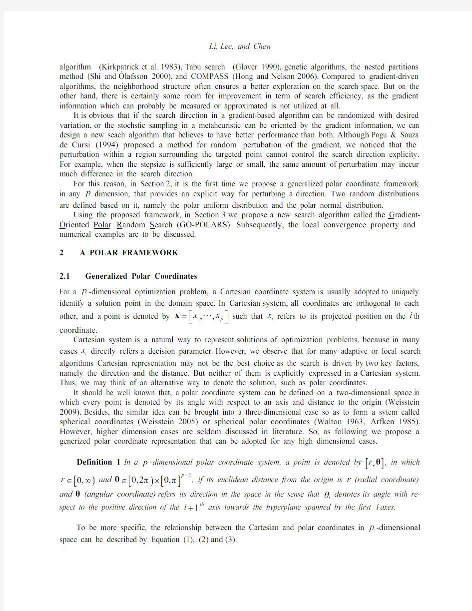
Definition 1In a p -dimensional polar coordinate system, a point is denoted by >@,r ?, in which > 0,r f and > >@20,20,p S S u ?, if its euclidean distance from the origin is r (radial coordinate) and ?(angular coordinate)refers its direction in the space in the sense that i T denotes its angle with re-
spect to the positive direction of the 1i th axis towards the hyperplane spanned by the first i axes.
To be more specific, the relationship between the Cartesian and polar coordinates in p -dimensional space can be described by Equation (1),(2)and (3).
r ,(1)111
sin j p j x r T ,(2)
11
cos sin for 2i i j p j i x p r i T T d d .
(3)An illustration for the generalized polar coordinate representation in the two and three dimensional space can be found in Figure 1. We note that the mapping from polar to the Cartesian coordinate system is almost one-to-one, and the degree of freedom remains p
in both representation.
Figure 1:An illustration of generalized polar coordinates (in 2D & 3D).
2.2Polar Uniform Sampling
With generalized polar coordinates we are able to denote a point in terms of the direction and distance re-ferring to a given position, which provides an advantage for algorithms to explicitly control their search process.But as mentioned in Section 1where the variation is involved in sampling a direction,random distribution need to be defined before we move to introduce the algorithm.First of all, we look at a uni-form case.
In a p -dimensional space, in order to uniformly sample a direction, we simply consider a hyperball with radius r around the origin. For all the points spread in the outermost layer, each of them should have equal opportunity to be sampled as the direction. From mathematical point of view, let ,f r ?be the probability density function, then within an infinitesimal space around the point >@,r ?, the probability for points to be sampled is
11,,,,p f r r T T w ?!.
By consensus of uniformity, this probability should be proportional to the volume of the infinitesimal space
1,,p V x x w w !, meaning there exists a function 0c r t such that
111,,,,,,p p f r r x x c r T T w w ?!!.
Further notice that the Jacobian determinant (Kaplan 1991)of the mapping from polar to Cartesian coor-dinate system is expressed as
111111
,1,,sin ,,,p p j j p p r j x x r J r T T T w w ?!!.So we derive the probability density function for a polar uniform distribution as in (4)and thus have Def-inition 2.Note that c r depends only on r and has to ensure the integral of ,f r ?on the domain equals to 1.
1111,sin
p j p j j f r c r r T ?.(4)
Definition 2A random point >@,r ?is said to be from a p -dimensional polar uniform distribution,
denoted as polar U p ,if its probability density function is given as in (4).
When enforce 1r ,i.e. let 0c r if 1r z ,the angular coordinate ?can be sampled uniformly
in the sense that >@polar 1,U p ? , which is illustrated by Figure 2.Since r is fixed and j T is independent
from each other, we can decompose the probability density function for each j as
1 for 1sin ,,,1
j j j j j f j p c T T !(5)where 112c S
and 01sin j j d c S T T 3for 2j t . As there is no close form for j c ,one of the method is to apply numerical approaches,such as acceptance-rejection method or Alias method (Vose 1999,Schwarz 2011)after discretization into small intervals,so that
the constant term can be ignored.Figure 2:Polar uniform distribution with 1r and 3,5,10p .
I n practice,some good properties can be observed. Since (5)is independent with dimension p , a
point >@polar 1,U p ? can be easily extended to 1polar U p by adding element p T sampled from distribution
with density
1sin p p p p p f c T T .
Moreover, considering (2)and (3),we notice that the newly added p T does not affect the relative val-
ues of previous i x ’s since all of them are simply scaled by sin p T , whereas the density in (5)only en-
sures that the new comer 1p x plays harmoniously with the early ones by maintaining the uniformity into the higher dimension.This property is important when we need to add controlled bias into the distribution,which is to be discussed later in 2.3.
Alternatively, we note that a multivariate normal distribution
2N ,I V 0with any V is a special case for polar uniform distribution when it is converted into the generalized polar coordinates (The proof is omitted due to the page limit). The sampled points can be easily standardized into unit vector by letting 1r before it can be applied in the steps following to be discussed. With this result, we can certainly simplify the random generator for polar uniform distribution.
2.3Concentrated Polar Distribution
Firstly,we consider a simple case, where we want the sampled direction to be concentrated around a giv-en direction d that coincides with the positive direction of the p th axis, i.e. p
d e .It means that, under the Cartesian representation only p x has a priority to choose larger value.Thus, using the property dis-
cussed in the later part of 2.2,we may have a point >@1polar 1U ,p ? ,and extend it to p -dimension by add-
ing 1p T where the distribution can be adjusted from (5),so that p x has higher chance to take large value without touching the ratio among the others.A typical way is to take the composite density with a trun-cated normal distribution with mean 0and variance 2V , i.e.,
21121101,sin p p p p p p f c V I T T T c (6)where 2222
2
022,2 for 0, for 2S T T V V V I T T S S T S d d d .Note that 11p p f T is defined on > 0,2S for 2p ,and >@0,S for 2p !.We refer it as the standard polar normal distribution as in Definition 3.
Definition 3A random point >@,r ?is said to be from a p -dimensional standard polar normal
distribution with variance 2V , denoted as 2polar N p V ,if 112polar ,U ,,p p r T T ao??! and 1p T distributed as in (6).
The procedure of generating >@
2polar 1N ,p V ? is described by Algorithm 1.Set V to different val-ues, then we have the illustration of sampled points shown by Figure 3. It is clear that similar to normal distribution, small V will have high density of samples around the given position p e .
An extreme case can be observed when 0V so that
210,0p V T I for all 10p T z , thus 10p T with probability 1, meaning that all sampled direction coincide with p e almost for sure. In an-other way, if V f , we have equal value of
20,1p V I T at all 1p T , thus the term cancelled out from (6).
In that case, polar polar N U p p f {.
Algorithm 1
Step 1:Let 1j .
Step 2:If 1j p , sample j T from its domain with density as in (5), then set 1j j .
Step 3:If 1j p , sample 1p T from its domain with proportional density as in (6), then stop and report 11,,p T T ao ???!; otherwise proceed to Step 3.
Step 4:Go to Step 2.
Figure 3:Standard polar normal distribution with 1r ,5p and 6,9,12V S S S .
Denote >@ Cart 1, d ?as the Cartesian conversion of >@1,?, we can analyze the expectation of d
(detailed steps are omitted due to the page limit),so as to derive Theorem 1. Later we will use its corol-lary to prove the local convergence property in 3.2.
Theorem 1For a unit vector 2polar N p V d given that V f ,we can always finds a scalar
@,0,1p V J depends only on p and V such that >@,E p p V J d e .
For the case where the given d is an arbitrary unit vector,a linear transformation can be applied such that every point obtained by Algorithm 1is reflected on a hyperline lies in the middle of d and p
e .In a reverse manner, we have Definition 4for the polar normal distribution.Figure 4is an illustration.
Definition 4A random point >@ Cart ,r d ?is said to be from a p -dimensional polar normal
distribution centered at unit vector d and variance 2V , denoted as 2polar N ,p V d ,if
2polar 22N T
p V d m m d m where 2p m d e .
Obviously, as the result of linear transformation, from Theorem 1we have Corollary 1.
Figure 4:Polar normal distribution with 12p i i |d e
e ,V S and 3,5,10p .
Corollary 1For a unit vector
2polar N ,p V d d given that V f ,we can always finds a scalar @,0,1p V J depends only on p and V such that >@,E p V
J d d d
.3
SEARCH ALGORITHM 3.1The Base Algorithm The Gradient Oriented Polar Random Search (GO-POLARS)is designed in an adaptive manner.At each iteration, the optimum estimate moves to a random direction with a step size which is guided by the gra-dient. Specifically, let p 4 \be the feasible region, the search algorithm can be described as following:
Algorithm 2
Step 1:(Initialization) Pick an initial guess 0? 4x
, and set 0k .Step 2:Generate a direction k d from
2polar ?N ,p k k V g x in which ?k g x is the gradient at ?k x .Step 3:Let new ???k k k k b x
x g x d .If new ? 4x and new ??k L L x x , set n w 1e ??k x x , other-wise 1??k k x
x .Step 4:Set 1k k . Go to Step 2.
Remark. The search procedure can be tuned by controlling the gain sequence k b and the direction variation sequence k V .In 3.2, we will discuss conditions in terms of k b and k V for the algorithm to con-
verge to a local optimum.
3.2Local Convergence Property
In literature, local convergence property of a stochastic algorithm is often shown by convergence theory of stochastic approximation (SA)(Spall 2003). And we notice that GO-POLARS shares some similarities with SA, such as both have estimates updated adaptively according to the gradient information with cer-tain noise. So in this subsection, we try to relate GO-POLARS to SA and conclude the convergence con-ditions for the sequence k b and k V .
We start with rewriting Step 3in Algorithm 2as an SA type, i.e., new ???k k k k a Y x
x x where ,k p k a b V J ,(7)
and ,??k k k k p Y V J g x
x d .(8)
Note that in a typical SA procedure,k a is the gain sequence and ???k k k k k k Y x
g x e x is an ap-proximation of gradient k g with error term k e .The “statistics”conditions for strong convergence can be drawn as in (9),(10),(11)and (12)(Blum 1954a,b;Nevel'son and Has'minskii 1973).
2000,0,a d ,n k k k k k k a a a a f f !o f f ||,
(9) *1/*in 0f T K K !x x x x Bg x for all 01K (10)
E 0k ao??e x for all x and k ,(11)
22E 1k c aod ??Y x x for all x and k and some 0c !.
(12)where B is some symmetric, positive definite matrix.By (7)and Corollary 1, condition in (9)can be substituted by (13)and (14).V f
(13)
2000,0,a d ,n k k k k k k b b b b f
f !o f f
||(14)While, condition in (11)can be derived from Corollary 1and (8). Similarly the condition in (12)can also be simplified as in (15)when Corollary 1and (8)are concerned.
2
2?1k c d g x x for all x and k and some 0c !.(15)
Thus we have the theorem for local convergence property.Note that the detailed proof is omitted due to the page limit.Theorem 2Given that conditions in (10),(13),(14)and (15)are satisfied,the search iterate ?k x
generated by Algorithm 2converges to a local optimum almost surely.
4NUMERICAL EXAMPLES
In this section, we compare GO-POLARS with several benchmark search algorithms including gradient-based search and metaheuristics local search.Besides, the hybrid of GO-POLARS with advanced stochas-tic search algorithms such as COMPASS will be illustrated as well.
4.1 A Benchmark Comparison
The Goldstein-Price’s function is a two-dimensional global optimization test function as defined in (16).Note that the global minimum occurs at *0,1 x with
*3L x , and several local minima occur as well. Set the search domain 24 \and assume that the gradient can be calculated at every 4x ,we used the function to compare the performance of GO-POLARS with steepest descent (SD)and simulated annealing method (SAN) as described in Table 1.
2221212121221212122212111914314633023183212483627L x x x x x x x x x x x x x x x x ao ?
?ao ??x (16)For fair comparison, we adopt a neighborhood structure setting in SAN that is similar to the GO-
POLARS iterate.But instead of choosing direction from a polar normal distribution oriented by the gradient, we let it be generated by a multivariate normal distrbibution that does not involve gradient. However, for comparison consistancy, the magnitude of gradient is used in determining the sample distance.In the experiment, we set 0.001k a k and 3V S for all occasions. Besdies, for SAN,the tempreture k T is set to be 500t k .As the experiement does not show significant difference when t is tuned to be any positive value, we set 1t for illustration.
Table 1:The overview of settings for testing algorithms.
The three algorithms can be corelated by starting with a same initial solution 0x that is randomly selected from >@2
2,2 , and run the algorithms until 500k . Repeat the process for 50replications, we then present the average *?k
L x in Figure 5. Note that in each replication, *?k x denotes the best solution
visited upon iteration k .Figure 5:Average *?k L x by different search algorithms.
It is obvious that the average performance of GO-POLARS across replication is superior than both SD and SAN. To analyze the reason, we notice that in SD only single direction is allowed to be sampled, but GO-POLARS ensures that all directions have a positive chance to be selected when 0V z , which certainly enlarged the pool of candidate solutions.I n SAN,the enlarged candidate pool is remianed, however, in order to filter it SAN arbitrarly rejects inferior samples after evaluation using an artificial tempreture paremeter k T . While in GO-POLARS, solutions on different directions can be filtered in advance with the gradient-oriented random distribution even before any evaluation.
4.2Hybrid with Stochastic Search
As stated in Section 1, almost all stochastic search algorithms involve random sampling within a specified neighborhood, where it is assumed that gradient information is not available. However, in the cases when gradient can be observed or estimated, we can apply GO-POLARS to help in sampling good solutions more efficiently. In the other hand, if GO-POLARS alone could not obtain desired efficiency, to integrate it with an advanced stochastic search will probably make the achievement.
Assume solutions are to be sampled from a convex set 4in which *? 4x
is the best known up-todate. We may sample *new ??r x x d where
*2polar ?N ,p V d g x and U 0,r R in which R is the maximum value of r that ensures new ? 4x
.We illustrate the concept using COMPASS (Hong and Nelson 2006), which is initially proposed for solving discrete optimization problems, but has been observed performing well also for contineous cases.The main idea of the algorithm is to construct a most-promissing-area after evaluation of all historical samples and in a new iteration retake samples within the area according to a given sampling scheme. For instance, Hong and Nelson (2006) suggest a Revised Mix-D (RMD) method aiming to generate samples almost uniformly. But later it is identified to be less efficient in solving high-dimensional problems, for which the Coordinate Sampling is proposed instead (Hong et al.2010).
>@2222212/1211001 with 4,4p i p i i i x x L x ao ??? 4 ?|x (17)
We apply the COMPASS on a high-dimension continuous test function as in (17). The function is in-itially proposed by Rosenbrock (1960)with 2p and extended by Moréet al.(1981)to higher dimension. Here, we use the setting 10p . Note that it has a unique optimum
*0L x occurring at *1,1,1 x !
.
Figure 6:Average *?k L x by COMPASS with different sampling schemes.
Two sampling schemes are compared in the test, namely the Coordinate Sampling (CS) and GO-POLARS sampling as in (17),for which the V is set to S and 6S respectively.Besides, the batch size of COMPASS, i.e., the number of solutions to be sampled in each iteration, is set to 1.
From the average
*?k L x drawn from 50replications (Figure 6), we conclude that compared with CS, the hybridized GO-POLARS provides a higher convergent rate and the rate increases as the sampling concentrates to the gradient direction (denoted by smaller V ).
In addition, by a long run study we found it almost impossible for CS converge to the uniqe optimum, simply due to the reason that CS is designed intently for discrete problems while in continuous cases the search could be trapped in the region where solution cannot be improved on any coordinate directions. Thus, for COMPASS to be applied in solving continuous problems, GO-POLARS is one of the only choices.
5CONCLUSION
In this paper, we reviewed two categories of search algorithms for optimization problems and suggest that incorporating randomness in utilizing gradient information will improve both gradient-based search and metaheuristics local search.A brand new algorithms GO-POLARS is built on this purpose using a gener-alized polar coordinate representation and associated random distributions. It has been shown that GO-POLARS has the strong local convergence property and works well in numerical examples either inde-pendently or hybridizing with sophisticated stochastic algorithms such as COMPASS.
Future study may address the adjustment of V and analyze how it affects the solutions quality versus search efficiency for different applications. The possibility to hybirdize GO-POLARS with other stochastic search algorithms can also be discussed. Besides, instead of gradient, other directional information based on the nature of respective problems can also be used to orient the polar random distribution. Then a large number of search and sampling algorithms can be developed based on the concept. Overall, with the promissing numerical results and the broad derivatives, we have plenty of reason to believe that GO-POLARS is openning a new era of polar search.
REFERENCES
Arfken , G. (1985). Spherical Polar Coordinates (3rd ed.). Orlando, FL: Academic Press.
Blum, J. R. (1954a). Approximation Methods Which Converge with Probability One. Annals of
Mathematical Statistics, 25, 382-386.
Blum, J. R. (1954b). Multidimensional Stochastic Approximation Methods. Annals of Mathematical
Statistics, 25, 737-744.
Debye, P. (1909, 12 1). N?herungsformeln für die Zylinderfunktionen für gro?e Werte des Arguments
und unbeschr?nkt ver?nderliche Werte des Index. Journal Name: Mathematische Annalen, 67(4), pp. 535-558.
Glover, F. (1990, July-August). Tabu Search; A Tutorial. Interfaces, 20(4), pp. 74-94.
Hong, L. J., & Nelson, B. L. (2006, January-February). Discrete Optimization via Simulation Using
COMPASS. Operations Research, 54(1), pp. 115-129.
Hong, L. J., Xu, J., & Nelson, B. L. (2010, September 21). Speeding up COMPASS for high-dimensional
discrete optimization via simulation. Operations Research Letters , pp. 550-555.
Kaplan, W. (1991). Advanced Calculus (4th ed. ed.). Redwood City, CA: Addison-Wesley.
Kiefer, J., & Wolfowitz, J. (1952). Stochastic Estimation of the Maximum of a Regression Function.
Annals of Mathematical Statistics, 23(3), pp. 462-466.
Kirkpatrick, S., Gelatt, C. D., & Vecchi, M. P. (1983, 5 13). Optimization by Simulated Annealing.
Science, 220(4598), pp. 671-680.
Matyas, J. (1965). Random Optimization. Automation and Remote Control, 26, 244-251.
Moré, J. J., Garbow, B. S., & Hillstrom, K. E. (1981). Testing Unconstrained Optimization Software.
ACM Transactions on Mathematical Software, 7(1), 17-41.
Neal, R. M. (2003). Slice Sampling. Annals of Statistics, 31(3), 705–767.
Nevel'son, M. B., & Has'minskii, R. Z. (1973, c1976). Stochastic Approximation and R ecursive Estimation.Providence, RI: American Mathematical Society.
Pogu, M., & Souza de Cursi, J. E. (1994). Global Optimizationby Random Perturbation of the Gradient Method with a Fixed Parameter. Journal of Global Optimization, 5, 159 -180.
Pohlheim, H. (2007, 1 15). Examples of Objective Functions.Retrieved 4 10, 2012, from GEATbx -The Genetic and Evolutionary Algorithm Toolbox for Matlab: https://www.doczj.com/doc/606819704.html,/download/GEATbx_ObjFunExpl_v38.pdf
Rosenbrock, H. H. (1960). An Automatic Method for Finding the Greatest or Least Value of a Function.
The Computer Journal, 3(3), 175-184.
Schwarz, K. (2011, 12 29). Darts, Dice, and Coins: Sampling from a Discrete Distribution. Retrieved 3 28, 2012, from https://www.doczj.com/doc/606819704.html,: https://www.doczj.com/doc/606819704.html,/darts-dice-coins/
Shi, L., & ólafsson, S. (2000, May-June). Nested Partitions Method for Global Optimization. Operations Research, 48(3).
Spall, J. C. (1998). An Overview of the Simultaneous Perturbation Method for Efficient Optimization.
Johns Hopkins APL Technical Digest, 19(4), pp. 482-492.
Spall, J. C. (2003). Introduction to stochastic search and optimization: estimation, simulation, and control.John Wiley & Sons, Inc.
Vose, M. D. (1999). A Linear Algorithm For Generating Random Numbers With a Given Distribution.
IEEE Transactions on Software Engineering, 17(9), 972-975.
Walton, J. J. (1963, March). Tensor calculations on computer: appendix. Communications of the ACM, 10(3), 183-186.
Weisstein, E. W. (2003, 9 5). Hypersphere. Retrieved 3 14, 2012, from MathWorld: https://www.doczj.com/doc/606819704.html,/Hypersphere.html
Weisstein, E. W. (2005, 10 26). Spherical Coordinates. Retrieved 3 14,2012, from MathWorld: https://www.doczj.com/doc/606819704.html,/SphericalCoordinates.html
Weisstein, E. W. (2009, 3 8). Polar Coordinates. Retrieved 3 14, 2012, from MathWorld: https://www.doczj.com/doc/606819704.html,/PolarCoordinates.html
AUTHOR BIOGRAPHIES
HAOBIN LI is a Ph.D. candidate in the Department of I ndustrial and Systems Engineering, National University of Singapore.He received his B.Eng. degree with 1st Class Honors in Industrial and Systems Engineering from National University of Singapore in 2009. His research interests include analytical methods of simulation,and multi-objective optimization. His email address is li_haobin@https://www.doczj.com/doc/606819704.html,.sg.
LOO HAY LEE is an Associate Professor and Deputy Head in the Department of Industrial and Systems Engineering, National University of Singapore. He received his B.S. (Electrical Engineering) degree from
the National Taiwan University in 1992 and his S. M. and Ph.D. degrees in 1994 and 1997 from Harvard University. He is currently a senior member of IEEE, a committee member of ORSS, and a member of INFORMS. His research interests include production planning and control, logistics and vehicle routing, supply chain modeling, simulation-based optimization, and evolutionary computation. His email address
is iseleelh@https://www.doczj.com/doc/606819704.html,.sg.
EK PENG CHEW is an Associate Professor and Deputy Head in the Department of Industrial and Sys-
tems Engineering, National University of Singapore. He received his Ph.D. degree from the Georgia Insti-
tute of Technology. His research interests include logistics and inventory management, system modeling
and simulation, and system optimization. His email address is isecep@https://www.doczj.com/doc/606819704.html,.sg.