
Search This Site
Browse the table of contents, or select an option from this menu:
Print this article (xxxK PDF)
A Primer for Panel Data Analysis
By Robert Yaffee
Panel data analysis is an increasingly popular form of longitudinal data analysis
among social and behavioral science researchers. A panel is a cross-section or group
of people who are surveyed periodically over a given time span.
In this article, we will consider a small sample of panel data analytic applications in
the social sciences. Then we will address the data structure for panel analysis.
Principal models of panel analysis will be summarized, along with some of their
relative advantages and disadvantages. We will discuss a test to determine whether
to use fixed or random effects models.
After a synopsis of methods of estimations tailored to different situations, we will
conclude with a brief discussion of popular software capable of performing panel
analysis.
Some Applications of Panel Analysis
Panel data analysis is a method of studying a particular subject within multiple sites,
periodically observed over a defined time frame. Within the social sciences, panel
analysis has enabled researchers to undertake longitudinal analyses in a wide
variety of fields. In economics, panel data analysis is used to study the behavior of
firms and wages of people over time. In political science, it is used to study political
behavior of parties and organizations over time. It is used in psychology, sociology,
and health research to study characteristics of groups of people followed over time.
In educational research, researchers study classes of students or graduates over
time.
With repeated observations of enough cross-sections, panel analysis permits the
researcher to study the dynamics of change with short time series. The combination
of time series with cross-sections can enhance the quality and quantity of data in
ways that would be impossible using only one of these two dimensions (Gujarati,
638). Panel analysis can provide a rich and powerful study of a set of people, if one Submit Click to choose an option...Go!
is willing to consider both the space and time dimension of the data.
The Panel Approach: An Overview
Panel data analysis endows regression analysis with both a spatial and temporal dimension. The spatial dimension pertains to a set of cross-sectional units of observation. These could be countries, states, counties, firms, commodities, groups of people, or even individuals. The temporal dimension pertains to periodic observations of a set of variables characterizing these cross-sectional units over a particular time span.
An example of a panel data set is a collection of three countries for which there are the same economic variables—such as personal expenditures, personal disposable income, and median household income, per capita income, personal disposable income, population size, unemployment, and employment—collected annually for ten years. This pooled data set, sometimes called time series cross-sectional data, contains a total of 3*10=30 observations. In other words, the three countries are followed for ten years and are sampled annually.
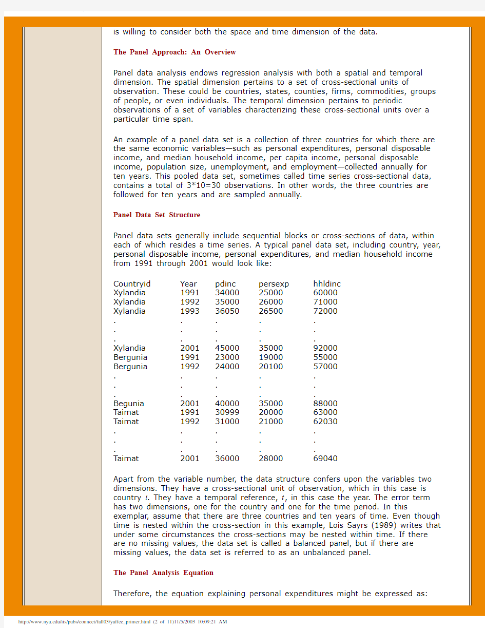
Panel Data Set Structure
Panel data sets generally include sequential blocks or cross-sections of data, within each of which resides a time series. A typical panel data set, including country, year, personal disposable income, personal expenditures, and median household income from 1991 through 2001 would look like:
Countryid Year pdinc persexp hhldinc
Xylandia1991340002500060000
Xylandia1992350002600071000
Xylandia1993360502650072000
.....
.....
.....
Xylandia2001450003500092000
Bergunia1991230001900055000
Bergunia1992240002010057000
.....
.....
.....
Begunia2001400003500088000
Taimat1991309992000063000
Taimat1992310002100062030
.....
.....
.....
Taimat2001360002800069040
Apart from the variable number, the data structure confers upon the variables two dimensions. They have a cross-sectional unit of observation, which in this case is country i. They have a temporal reference, t, in this case the year. The error term has two dimensions, one for the country and one for the time period. In this exemplar, assume that there are three countries and ten years of time. Even though time is nested within the cross-section in this example, Lois Sayrs (1989) writes that under some circumstances the cross-sections may be nested within time. If there are no missing values, the data set is called a balanced panel, but if there are missing values, the data set is referred to as an unbalanced panel.
The Panel Analysis Equation
Therefore, the equation explaining personal expenditures might be expressed as:
Types of Panel Analytic Models
There are several types of panel data analytic models. There are constant coefficients models, fixed effects models, and random effects models. Among these types of models are dynamic panel, robust, and covariance structure models. Solutions to problems of heteroskedasticity and autocorrelation are of interest here. We will try to summarize some of the prominent aspects of this kind of methodology, but first we need to consider the data structure.
The Constant Coefficients Model
One type of panel model has constant coefficients, referring to both intercepts and slopes. In the event that there is neither significant country nor significant temporal effects, we could pool all of the data and run an ordinary least squares regression model. Although most of the time there are either country or temporal effects, there are occasions when neither of these is statistically significant. This model is sometimes called the pooled regression model.
The Fixed Effects Model (Least Squares Dummy Variable Model)
Another type of panel model would have constant slopes but intercepts that differ according to the cross-sectional (group) unit—for example, the country. Although there are no significant temporal effects, there are significant differences among countries in this type of model. While the intercept is cross-section (group) specific and in this case differs from country to country, it may or may not differ over time. These models are called fixed effects models.
After we discuss types of fixed effects models, we proceed to show how to test for the presence of statistically significant group and/or time effects. Finally, we discuss the advantages and disadvantages of the fixed effects models before entertaining alternatives. Because i-1 dummy variables are used to designate the particular country, this same model is sometimes called the Least Squares Dummy Variable model (see Eq. 2).
Another type of fixed effects model could have constant slopes but intercepts that differ according to time. In this case, the model would have no significant country differences but might have autocorrelation owing to time-lagged temporal effects. The residuals of this kind of model may have autocorrelation in the process. In this case, the variables are homogenous across the countries. They could be similar in region or area of focus. For example, technological changes or national policies would lead to group specific characteristics that may effect temporal changes in the variables being analyzed. We could account for the time effect over the t years with t-1 dummy variables on the right-hand side of the equation. In Equation 3, the dummy variables are named according to the year they represent.
There is another fixed effects panel model where the slope coefficients are constant, but the intercept varies over country as well as time. In Equation 4, we would have a regression model with i-1 country dummies and t-1 time dummies. The model could be specified as follows:
Another type of fixed effects model has differential intercepts and slopes. This kind of model has intercepts and slopes that both vary according to the country. To formulate this model, we would include not only country dummies, but also their interactions with the time-varying covariates (Eq. 5).
In this model, the intercepts and intercepts vary with the country. The intercept for Country1 would be a1. The intercept for Country2 would also include an additional intercept, a2, so the intercept for Country2 would be a1+a2. The intercept for Country3 would include an additional intercept. Hence, its intercept would be a1 +
a3. The slope for PDI2it with Country2 would be b2 + b4, while the slope for PDI2it with Country3 would be b2 + b5. One could similarly compute the slope for HHinc3it with Country2 as b3 + b6. In this way, the intercepts and slopes vary with the country.
There is also a fixed effects panel model in which both intercepts and slopes might vary according to country and time. This model specifies i-1 Country dummies, t-1 Time Dummies, the variables under consideration and the interactions between them. If all of these are statistically significant, there is no reason to pool. The degree of freedom consumption leaves this model with few degrees of freedom to test the variables. If there are enough variables, the model may not be analyzable.
Fixed Effect Hypothesis Testing
We may wish to hierarchically test the effects of the fixed effects model. We use the pooled regression model as the baseline for our comparison. We first test the group (country) effects. We can perform this significance test with an F test resembling the structure of the F test for R2 change.
Here T=total number of temporal observations. n=the number of groups, and
k=number of regressors in the model. If we find significant improvements in the R2, then we have statistically significant group effects.
We also want to test for the time effects. This can be done by a contrast, using the first or last time point as a reference. We assume that the sum of the time effects is equal to zero. Referring to Equation 3, we use a contrast, which is a paired t test between the reference and test value. Greene (2003) expresses Eq. 3 more generally as:
In this formulation, the group effects are the αi s and the time effects are the γi s.
One can obtain least squares estimates for ys and xs with:
Greene (2003) formulates the time effects by:
We can test for group, time, and interaction effects, assuming that we have not consumed all of our degrees of freedom. We hope to see an improvement in the R2 without a problem with autocorrelation. If the panels are unbalanced, adjustments to the total counts are made. By using instead of nT to account for the total number of observations, proper variances and F tests are computed. Hence, the unbalanced panels are easy to accommodate.
Because fixed effects estimators depend only on deviations from their group means, they are sometimes referred to as within-groups estimators (Davidson and MacKinnon, 1993). If the cross-sectional effects are correlated with the regressors, then the cross-sectional effects will be correlated with the group means. Ordinary least squares estimation on the pooled sample would be inconsistent, even though the within-groups estimator would be consistent. If, however, the fixed effects are uncorrelated with the regressors, the within-groups estimator will not be efficient. If there is only variation between the group means, then it would be permissible to use the between-groups estimator, but this would inconsistent if the cross-sectional errors are correlated with the group means of the regressors (Davidson and MacKinnon, 1993).
Fixed Effects Pros and Cons
Fixed effects models are not without their drawbacks. The fixed effects models may frequently have too many cross-sectional units of observations requiring too many dummy variables for their specification. Too many dummy variables may sap the model of sufficient number of degrees of freedom for adequately powerful statistical tests. Moreover, a model with many such variables may be plagued with multicollinearity, which increases the standard errors and thereby drains the model of statistical power to test parameters. If these models contain variables that do not vary within the groups, parameter estimation may be precluded. Although the model residuals are assumed to be normally distributed and homogeneous, there could easily be country-specific (groupwise) heteroskedasticity or autocorrelation over time that would further plague estimation.
The one big advantage of the fixed effects model is that the error terms may be correlated with the individual effects. If group effects are uncorrelated with the group means of the regressors, it would probably be better to employ a more parsimonious parameterization of the panel model.
The Random Effects Model
Prof. William H. Greene calls the random effects model a regression with a random constant term (Greene, 2003). One way to handle the ignorance or error is to assume that the intercept is a random outcome variable. The random outcome is a function of a mean value plus a random error. But this cross-sectional specific error term v i, which indicates the deviation from the constant of the cross-sectional unit (in this example, country) must be uncorrelated with the errors of the variables if this is to be modeled. The time series cross-sectional regression model is one with an intercept that is a random effect.
Under these circumstances, the random error v i is heterogeneity specific to a cross-sectional unit—in this case, country. This random error v i is constant over time. Therefore, The random error e it is specific to a particular observation. For v i to be properly specified, it must be orthogonal to the individual effects. Because of the separate cross-sectional error term, these models are sometimes called one-way random effects models. Owing to this intrapanel variation, the random effects model has the distinct advantage of allowing for time-invariant variables to be included among the regressors.
Error Components Models
If, however, the random effects model depends on both the cross-section and the time series within it, the error components (sometimes referred to as variance components) models are referred to as a two-way random effects model. In that case, the error term should be uncorrelated with the time series component and the cross-sectional (group) error. The orthogonality of these components allows the general error to be decomposed into cross-sectional specific, temporal, and individual error components.
The component, v i, is the cross-section specific error. It affects only the observations in that panel. Another, e t, is the time-specific component. This error
component is peculiar to all observations for that time period, t. The third ηit affects only the particular observation. These models are sometimes referred to as two-way random effects models (SAS, 1999).
The Random Parameters Model
In the Hildreth, Houck, and Swamy random coefficient model, the parameters are allowed to vary over the cross-sectional units. This model allows both random intercept and slope parameters that vary around common means. The random parameters can be considered outcomes of a common mean plus an error term, representing a mean deviation for each individual. This model assumes neither heteroskedasticity nor autocorrelation within the panels to avoid complicating the covariance matrix.
In multilevel models pertaining to students, schools, and cities, there can be individual student, school, and city random error terms as well. There can also be cross-level interactions within these hierarchical models.
Dynamic Panel Models
If there is autocorrelation in the model, it is necessary to deal with it. One can apply one or more of the several tests for residual autocorrelation. The Durbin-Watson test for first-order autocorrelation in the residuals was modified by Bhargava et al. to handle balanced panel data. Baltagi and Wu (1999) modified it further to handle unbalanced panel and equally spaced data (STATA, 2003). There may be panel specific autocorrelation or there may be common autocorrelation across all panels. There are provisions for specifying the type of autocorrelation. Alternatively, an autoregression on lags of the residuals may indicate the presence or absence of autocorrelation and the need for dynamic panel analysis.
If there is autocorrelation from one temporal period to another, it is possible to analyze the "differences in differences" of these observations, using the first or last as a baseline (Wooldridge, 2002). If autocorrelation inheres across these observations, the model may be first partial differenced to control for the autocorrelation effects on the residuals (Greene, 2002). Arellano and Bond introduced lagged dependent variables into their model to account for dynamic effects. The lagged dependent variables can be introduced to either fixed or random effects models. Their inclusion assumes that the number of temporal observations is greater than the number of regressors in the model.
Even if one assumes no autocorrelation, problems from the correlation of the lagged endogenous and the disturbance term may plague the analysis. Bias can result especially when the sample is finite or small. If one uses general methods of moments, with instrumental variables, the use of the proxy variables or instruments may circumvent problems with correlations of errors. Moreover, there are a large number of instruments provided by lagged variables. GMM with these instruments and larger orders of moments can be used to obtain additional efficiency gains.
Another approach to deal with autocorrelation in the random errors is the Parks method. The model assumes an autoregressive error structure of the first order along with contemporaneous correlation among the cross-sections and this model is estimated by a two-state generalized least squares procedure (SAS Institute, 1999).
Panel data models with generalized estimating equations can handle higher order panel data analysis.
Robust Panel Models
There are a number of problems that plague panel data models. Outliers can bias regression slopes, particularly if they have bad leverage. These outliers can be downweighted with the use of M-estimators in the model. Heteroskedasticity problems arise from groupwise differences, and often taking group means can remove heteroskedasticity. The use of a White heteroskedasticity consistent covariance estimator with ordinary least squares estimation in fixed effects models can yield standard errors robust to unequal variance along the predicted line (Greene, 2002; Wooldridge, 2002).
Sometimes autocorrelation inheres within the panels from one time period to another. Some problems with dynamic panels that contain autocorrelation in the residuals are handled with a Prais-Winston transformation or a Cochrane-Orcutt transformation that amounts to a first partial differencing to remove the bias from the autocorrelation. Arellano, Bond, and Bover developed one and two step general methods of moments (GMM) estimators for panel data analysis. GMM is usually robust to deviations of the underlying data generation process to violations of heteroskedasticity and normality, insofar as they are asymptotically normal but they are not always the most efficient estimators.
If there is autocorrelation in the models, one can obtain a weight-adjusted combination of the White and Newey-West estimator to handle both the heteroskedasticity and the autocorrelation in the model.
Specification Tests: the Quandary of Random or Fixed Effect Models
The Hausman specification test is the classical test of whether the fixed or random effects model should be used. The research question is whether there is significant correlation between the unobserved person-specific random effects and the regressors. If there is no such correlation, then the random effects model may be more powerful and parsimonious. If there is such a correlation, the random effects model would be inconsistently estimated and the fixed effects model would be the model of choice.
The test for this correlation is a comparison of the covariance matrix of the regressors in the LSDV model with those in the random effects model. The null hypothesis is that there is no correlation. If there is no statistically significant difference between the covariance matrices of the two models, then the correlations of the random effects with the regressors are statistically insignificant. The Hausman test is a kind of Wald χ2 test with k-1 degrees of freedom (where k=number of regressors) on the difference matrix between the variance-covariance of the LSDV with that of the Random Effects model. SAS, SPSS and LIMDEP all contain the Hausman specification test. LIMDEP also contains the Bhargarva and Sargan Test (1983).
Model Estimation
Models have to be estimated by methods that handle the problems afflicting them. A constant coefficients model with residual homogeneity and normality can be estimated with ordinary least squares estimation (OLS). As long as there is no groupwise or other heteroskedastic effects on the dependent variable, OLS may be used for fixed effects model estimation as well (Sayrs, 1989). For OLS to be properly applied, the errors have to be independent and homoskedastic. Those conditions are so rare that is often unrealistic to expect that OLS will suffice for such models (Davidson and MacKinnon, 1993).
Heteroskedastic models are usually fitted with estimated or feasible generalized least squares (EGLS or FGLS). Heteroskedasticity can be assessed with a White or a Breusch-Pagan test. For the most part, fixed effects models with groupwise
heteroskedasticity cannot be efficiently estimated with OLS. If the sample size is large enough and autocorrelation plagues the errors, FGLS can be used. Random sampling and maximum likelihood iterated by generalized least squares have also been used (Greene, 2002). Beck and Katz (1995) reportedly found that if the sample size is finite or small, the total number of temporal observations must be as large as the number of panels; moreover they reportedly found that OLS with panel corrected errors provided more efficient estimation than FGLS (Greenberg, 2003; STATA, 2003).
If the model exhibits autocorrelation and/or moving average errors, first differences (Wooldridge, 2002) or GLS corrected for ARMA errors can be used (Sayrs, 1989). Hausman and Taylor (1981) have used weighted instrumental variables, based only on the information within the model, for random effects estimation to be used when there are enough instruments for the modeling. The instrumental variables, which are proxy variables uncorrelated with the errors, are based on the group means. The use of these instrumental variables allows researchers to circumvent the inconsistency and inefficiency problems following from correlation of the individual variables with the errors.
For dynamic panels with lagged dependent variables, Arellano, Bond, and Bover have used general methods of moments, which are asymptotically normal (Wooldridge, 2002). With greater numbers of moment conditions, they are able to handle some missing data and they can attain gains in efficiency as long as there are three or four periods of data (Greene, 2002).
Another estimation procedure was developed by Arnold Zellner, called seemingly unrelated regression (SUR) requires that the number of explanatory variables in each cross-section is the same. In the SUR approach, variables are transformed with a form of Cochrane-Orchutt correction to model the autocorrelation. Feasible generalized least squares is used to estimate a covariance matrix. The parameter estimates are also modeled. The process is iterated until the errors are minimized.
LIMDEP 8 (Greene, 2002) has its own protocol for estimating random parameter models, including the limited dependent variable models. The limited dependent variable models are population averaged models. In LIMDEP, the estimation for such models begins with an OLS estimation of starting values and then proceeds to simulation with Halton draws. This procedure, Greene maintains, is generally faster than the quadrature estimation used by Stata. When the panels are large in number and size, it may be the only timely method for estimation.
If there are enough temporal observations, they can use either the lagged levels or lagged differences as instruments, while the other variables serve as their own instruments in an extension. If group sizes are larger than 20 and the autocorrelation is higher than 0.4, the random effects quadrature algorithms can bog down or even fail to converge (STATA, 2003).
Robust estimation, when one has heteroskedasticity, autocorrelation, or outliers to contend with, may be performed with the general methods of moments and combination of White and Newey-West estimators to obtain robust panel standard errors. Arellano, Bond, and Bover have used GMM in their models and these are incorporated into LIMDEP version 8 and Stata version 8 special edition. GMM models tend to be robust with respect to heteroskedasticity and nonnormality. Professors Jeffrey Powell and Kenneth Chay (2003), University of California at Berkeley, have applied robust estimation to semiparametric censored panel data regression analysis (https://www.doczj.com/doc/6f4826912.html,/~kenchay/ftp/binresp/jepfinal.pdf, September 21, 2003). They have used least absolute deviations estimation, a form of robust modeling that is relatively invulnerable to outlier distortion, to apply to censored data.
Statistical Packages
Among those statistical packages that excel in programs for panel data analysis are
LIMDEP, STATA, and SAS. Although all three packages have procedures dedicated to panel data analysis, LIMDEP and STATA appear to have a particularly rich variety of panel analytic procedures. All three packages have fixed and random effects models, can handle balanced or unbalanced panels, and have one- or two-way random and fixed effects models. Although LIMDEP and STATA have the both Hausman and Sargan tests for specification, SAS has only the Hausman specification test. Both LIMDEP and STATA have the Hausman and Taylor estimator for random effects. All three packages have procedures that can correct for autocorrelation in the models. LIMDEP and STATA have Arellano, Bond and Bover's estimator for dynamic panel models, whereas SAS uses the Parks method. LIMDEP, STATA, and SAS procedures can handle groupwise heteroskedasticity in the random effects model. LIMDEP and STATA have the Hildreth, Houck, and Swamy random coefficients model. Stata has xtreg for performing a random coefficient analysis with only a random intercept. When more than one random coefficient has to be analyzed, one can use the gllamm (generalized linear latent and mixed models) procedure (Twisk, 2003). SAS can perform this kind of analysis with its Mixed procedure. STATA and LIMDEP have procedures for panel corrected standard errors. SAS has a variance component moving average (De Silva) procedure.
Both LIMDEP and STATA have procedures for limited dependent panel data analysis. They have poisson, negative binomial, logit, probit, and complimentary log-log panel models with either fixed or random effects. Although Stata can model these limited dependent variable models as random effects or population averaged models (with the exceptions of the poisson and negative binomial models, which can be modeled as fixed, random, or population averaged models), LIMDEP can model them as either fixed or random effects models. Both can analyze panel stochastic frontier models.
STATA and LIMDEP have cross-sectional time series population average generalized estimating equation models as well. These model use a variety of link functions (identify, log, logit, probit, negative binomial, and complimentary log-log), distribution families (Gaussian, inverse Gaussian, binomial, poisson, negative binomial, and gamma) and working correlation matrix structures (independent, exchangeable, autoregressive, stationary, structured, and unstructured) that provide for a flexible modeling for equally or unequally spaced correlation structures of panel data with iterated reweighted least squares estimation. LIMDEP has a procedure for the random parameters model and for a Latent Class Linear Regression model.
References
Davidson, R. and MacKinnon, J.G. (1993). Estimation and Inference in Econometrics. New York: Oxford University Press, pp. 320, 323.
Greene, W. H. (2002). LIMDEP, version 8.0. Econometric Modeling Guide, Vol 1. Plainview, NY: Econometric Software, Inc., pp.E14-9 - E14-11.
Greene, W. H. (2003). Econometric Analysis. 5th ed. Upper Saddle River: Prentice Hall, pp. 285, 291, 293, 304.
Greenberg, D. Longitudinal Data Analysis, personal communication, September 6, 2003, referring to the research of Nathaniel Beck.
Gujarati, D. (2003). Basic Econometrics. 4th ed. New York: McGraw Hill, pp. 638-640.
Greene, W. H. (2003). LIMDEP Version 8 Econometric Modeling Guide, Vol. 1. Plainview, NY: Econometric Software, pp. E8_1-E8_98; E8_26-E8_30.
Powell, J. and Chay, K. (2003). Semiparametric Censored Regression Models. Downloaded from World Wide Web, September 21, 2003) from http://elsa.berkeley.
edu/~kenchay/ftp/binresp/jepfinal.pdf.
SAS Institute (1999). SAS User's Guide, Version 8. Vol 2. Cary, NC: SAS Institute. pp. 1111, 1113, 1114.
Sayrs, L. (1989). Pooled Time Series Analysis. Newbury Park, Ca: Sage, pp.10, 32.
Stata (2003). Cross-Sectional Time Series. College Station, Texas: Stata Press, pp. 10, 62, 93, 224.
Twisk, Jos. W. (2003). Applied Longitudinal Data Analysis for Epidemiology. New York: Cambridge University Press. pp. 250-251.
Woolridge, J. (2002). Econometric Analysis of Cross-Section and Panel Data. MIT Press, pp. 130, 279, 420-449.
Author Biography
Robert Yaffee, Ph.D. is a statistician within the Social Sciences, Statistics & Mapping Group of ITS' Academic Computing Services. He can be reached at robert.
yaffee@https://www.doczj.com/doc/6f4826912.html,.
Page last reviewed: November 5, 2003. All content ? New York University.
Questions or comments about this site? Send e-mail to: its.connect@https://www.doczj.com/doc/6f4826912.html,.