
Personalized Route Recommendation using
Big Trajectory Data
Jian Dai??,Bin Yang?,Chenjuan Guo§,Zhiming Ding?
?University of Chinese Academy of Sciences,Beijing,China
?Institute of Software,Chinese Academy of Sciences,Beijing,China
daijian@https://www.doczj.com/doc/6413307232.html,
?Department of Computer Science,Aalborg University,Denmark
byang@cs.aau.dk
§Department of Computer Science,Aarhus University,Denmark
cguo@cs.au.dk
Abstract—When planning routes,drivers usually consider a multitude of different travel costs,e.g.,distances,travel times, and fuel consumption.Different drivers may choose different routes between the same source and destination because they may have different driving preferences(e.g.,time-ef?cient driving v.s. fuel-ef?cient driving).However,existing routing services support little in modeling multiple travel costs and personalization—they usually deliver the same routes that minimize a single travel cost (e.g.,the shortest routes or the fastest routes)to all drivers.
We study the problem of how to recommend personalized routes to individual drivers using big trajectory data.First,we provide techniques capable of modeling and updating different drivers’driving preferences from the drivers’trajectories while considering multiple travel costs.To recommend personalized routes,we provide techniques that enable ef?cient selection of a subset of trajectories from all trajectories according to a driver’s preference and the source,destination,and departure time speci?ed by the driver.Next,we provide techniques that enable the construction of a small graph with appropriate edge weights re?ecting how the driver would like to use the edges based on the selected trajectories.Finally,we recommend the shortest route in the small graph as the personalized route to the driver.Empirical studies with a large,real trajectory data set from52,211taxis in Beijing offer insight into the design properties of the proposed techniques and suggest that they are ef?cient and effective.
I.I NTRODUCTION
Traveling plays an important role in our lives and more and more people choose to use vehicles for traveling.To facil-itate route selection,a variety of navigation services become available and are able to recommend routes when a source, a destination,and sometimes,a departure time,are given. However,the routes recommended by existing navigation services are not always preferred by all drivers.For example, a recent study suggests that the routes provided by a leading navigation service often fail to agree with the routes chosen by local drivers[5].
The reason of the disagreement may be two-fold.First, most of the existing navigation services only consider a limited number of travel costs,e.g.,distance or travel time,and return routes that minimize a single travel cost,e.g.,shortest routes or fastest routes.In contrast,drivers may consider a multitude of different travel costs.For instance,due to an increasing public awareness of environmental protection and high fuel pricing, many drivers increasingly consider fuel consumption[1],in addition to travel times and travel distances.
Second,existing navigation services provide all drivers with the same routes(e.g.,shortest routes or fastest routes) and they do not take into account individual drivers’driving preferences(e.g.,time-ef?cient driving,fuel-ef?cient driving, or some trade-off between them).
These motivate us to study how to model drivers’driving preferences and to provide personalized routes to different drivers,which can better satisfy drivers’needs.
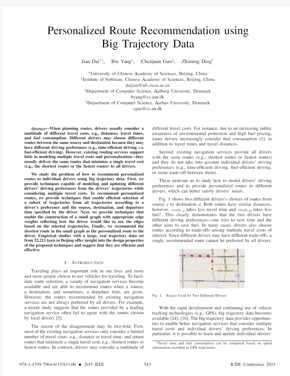
Fig.1shows two different drivers’s choices of routes from source s to destination d.Both routes have similar distances, however,route A takes less travel time and route B takes less fuel1.This clearly demonstrates that the two drivers have different driving preferences—one tries to save time and the other aims to save fuel.In many cases,drivers also choose routes according to trade-offs among multiple travel costs of interest.Since different drivers may have different trade-offs,a single,recommended route cannot be preferred by all
drivers.
Fig.1.Routes Used by Two Different Drivers
With the rapid development and continuing use of vehicle tracking technologies(e.g.,GPS),big trajectory data becomes available[24],[16].The big trajectory data provides opportuni-ties to enable better navigation services that consider multiple travel costs and individual drivers’driving preferences.In particular,it is possible to learn and update individual drivers’1Travel time and fuel consumption can be computed based on speed information recorded in GPS trajectories.
driving preferences according to their trajectories.Further, when a driver plans a route,the trajectories used by those drivers who have similar driving preferences to the driver can be utilized to suggest personalized route to the driver.
To the best of our knowledge,this paper is the?rst to explore the possibility of providing personalized route recom-mendation using big trajectory data.Speci?cally,the paper makes four contributions.First,it proposes a novel problem on personalized route recommendation based on big trajectory data.Second,it proposes techniques to model and update driving preferences from drivers’trajectories.Our driving preference model can support arbitrary number of travel costs of interest and distributions of cost ratios.Third,it proposes a local and a global route recommendation algorithms to recommend personalized routes to drivers.The algorithms are novel because(a)reference trajectories are selected from big trajectories while considering driving preferences;(b)local and global route recommendations are proposed to support different routing scenarios.Fourth,it reports on comprehensive experiments conducted on a substantial,real trajectory data set.These elicit design properties of the paper’s proposals and characterize the ef?ciency and the effectiveness of the personalized route recommendation.
The remainder of the paper is structured as follows.Sec-tion II de?nes the driving preference and formalizes the prob-lem.Section III describes the indexes.Section IV describes the retrieval of reference trajectories.Section V presents the personalized route recommendation methods.Section VI re-ports on the empirical evaluation.Section VII reviews related work and Section VIII concludes the paper.
II.P ROBLEM F ORMULATION
A.Basic Concepts
De?nition1:A road network is a directed graph G= (V,E),where V is a vertex set and E?V×V is an edge set.
A vertex v i∈V denotes a road junction or a road end.An edge e k=(v i,v j)∈E represents a directed road segment, indicating that travel is possible from its starting vertex v i to its ending vertex v j.To ease the following discussions,we denote the starting and ending vertices of edge e k as e k.s and e k.d,respectively.
De?nition2:A Route R= r1,r2,···,r A is a sequence of edges,where r i∈E and r i=r j if i=j.The consecutive edges must share a vertex,i.e.,r i.d=r i+1.s where1 i De?nition3:A trajectory T= t1,p1 , t2,p2 ,..., t B,p B is a sequence of GPS records pertaining to a trip, where each GPS record t i,p i indicates that a vehicle is at location p i at timestamp t i.Further,the GPS records in a trajectory are ordered by their timestamps,i.e.,t i De?nition4:A trajectory is associated with a cost vector costs(T)= c1,c2,...,c N ,where cost value costs(T).c i corresponds to the i-th cost of using T. In this paper,we consider N=3types of costs—travel distance(i.e.,costs(T).c1),travel time(i.e.,costs(T).c2), and fuel consumption(i.e.,costs(T).c3),which are the three most important factors while planning trips[21].However,the proposed techniques also apply to cases with arbitrary N. Given a trajectory T,the travel distance of T can be obtained by?rst map-matching the GPS records in T to road segments and then summing up the lengths of the road segments.The travel time of T can be obtained by computing the difference between the timestamps of the last and?rst GPS records in T.The fuel consumption of T can be derived from the length and the average speed of the trajectory,which can be derived from the GPS records in T,using appropriate vehicular environmental impact models[9]. B.Modeling Driving Preferences De?nition5:Given two travel costs of trajectory T,say costs(T).c i and costs(T).c j,the preference ratio w.r.t.the two travel costs is pr i,j=costs(T).c i costs(T).c j . Suppose costs(T)= 6.5km,13min,0.58l ,the prefer-ence ratio w.r.t.the distance and travel time is pr1,2=6.5 13 . De?nition6:A driver is associated with a driving prefer-ence vector P= p1,p2,...,p M that consists of M random variables,where M= N 2 and each random variable p i describes the distribution of a preference ratio. For example,when considering N=3travel costs,a driver’s driving preference vector has M= 3 2 =3random variables,which describe the distributions of the preference ratios w.r.t.distance v.s.travel time,distance v.s.fuel con-sumption,and travel time v.s.fuel consumption,respectively. Given a driver’s historical trajectories,the driver’s driving preference vector can be derived as follows.We consider a preference ratio at a time.For each trajectory,the preference ratio of the trajectory can be computed according to De?ni-tion5.Thus,we obtain a collection of preference ratio values from the driver’s all trajectories.Next,a random variable describing the distribution of the values in the collection can be obtained.Finally,M random variables corresponding to the distributions of the M preference ratios become available, which in turn construct the driver’s driving preference vector. A Gaussian Mixture Model(GMM)is employed to de-scribe the distribution of a random variable in the driving preference vector P,because a GMM is capable of describing any complex probability functions[3],[21].Given a col-lection of values,the GMM can be derived using existing algorithms[19].Thus,P is actually a sequence of M GMMs. De?nition7:Given a driver’s driving preference vec-tor P= p1,p2,...,p M ,a Personalized Satisfaction Score Function F quanti?es the degree of satisfaction of a trajectory T for the driver.In particular,F(T,P)= M i=0 ?T i+? ?T i ?? p i(c)dc,where?T i represents the preference ratio of T w.r.t.p i,?is a small real value to form a narrow?-neighborhood[?T i??,?T i+?].The higher value returned by function F,the more satisfactory the trajectory is for the driver. Assume we only consider two travel costs (i.e.,fuel con-sumption and travel time)and thus only one preference ratio in driving preference vector P = p 1 .Fig.2shows that the pdfs of the preference ratio random variable p 1for two different drivers driver1and driver2in our real trajectory data set.Consider two trajectories T 1and T 2using two different routes but connecting the same source-destination.We ?rst compute their corresponding preference ratios and construct their ?-neighborhoods I 1and I 2,respectively,as shown in Fig.2.Clearly,for driver 1,the route used by T 1is preferred than that by T 2because F (T 1,P driver 1)>F (T 2,P driver 1).Similarly,the route used by T 2is preferred by driver 2 . (a)pdf of p 1,driver 1 (b)pdf of p 1,driver 2 Fig.2. Evaluating Personalized Satisfaction Score Functions C.Updating Driving Preferences A driver’s driving preference vector typically does not keep invariant,especially when considering a relatively long time span.For example,when a driver’s ?nancial situation changes,e.g.,having a high salary job after graduation from university,the driver’s driving preference vector may be changed signi?-cantly. To timely update the random variables in a driver’s driving preference vector,we try to identify when a driver’s driving preference vector starts changing signi?cantly.Once the driver produces a new trajectory T ,the trajectory is called signi?-cantly different from the driver’s driving preference vector P if its personalized satisfaction score is smaller than a threshold ξ,i.e.,F (P,T )<ξ.Here,threshold ξis introduced to play a role which is similar to the p -value in the conventional statistical signi?cance testing [8].Once such a signi?cantly different trajectory is identi?ed,we start accumulate the driver’s trajec-tories and build a new driving preference vector P according to the procedure described in Section II-B.D.Problem Formulation De?nition 8:A Personalized Route Recommendation (PRR)query,denoted as PRR (v s ,v d ,t,P ),takes as input a source vertex v s ,a destination vertex v d ,a departure time t ,and a driver’s driving preference vector P .The query returns the shortest route in a reference graph .The reference graph is a sub-graph of the road network,where the edges satisfy the following two features:(1)the edges were traversed by the trajectories whose drivers have driving preferences similar to P and that went through from v s to v d and occurred at a similar departure time t of a day;(2)an edge in the reference graph is associated with a weight ,where a lower weight value indicates that more drivers prefer to use the edge. The construction of reference graph is discussed in Sec-tion V. E.Framework Overview Fig.3gives an overview of the framework for answering personalized route recommendation queries.The framework consists of three major modules,index construction ,reference trajectories retrieval ,and personalized route recommendation . Inverted Trajectory Index for Trajectories Reference trajectories retrieval Spatial filter Temporal filter Index Consturction Personalized route recommendation Local route computation Global routes computation Preference filter Grid Index for Road Network Fig.3.Framework Overview The index construction module is responsible for managing the trajectories and the road network where the trajectories oc-curred.It builds an inverted trajectory index for the trajectories and a grid index for the road network. Given the input parameters of a PRR query (i.e.,a source,a destination,a departure time,and a driving preference vector),the reference trajectories retrieval module applies various ?lers,including a spatial ?lter ,a temporal ?lter ,and a preference ?lter ,to retrieval a set of reference trajectories that are highly relevant to the query.When retrieving the reference trajectories,the two indexes built in the index construction module are used to facilitate the retrieving process. The personalized route recommendation takes as input the reference trajectories returned by the trajectories retrieval module.Two strategies,local route computation and global route computation ,are applied on the reference trajectories to compute the personalized route satisfying the driving prefer-ence vector. III. I NDEX C ONSTRUCTION A.Indexing the Trajectories Recall that map matching [17]is able to map a GPS record in a trajectory to a speci?c location on an edge in the underlying road network.Thus,map matching associates trajectories with edges in the road network. A common operation in the later reference trajectories retrieval model is to retrieve all the trajectories that occurred on a given edge.To ef?ciently support this operation,an Inverted Trajectory Index (ITI)is constructed to record the relationships between edges and the trajectories occurred on the edges.The ITI contains a set of entries where each entry corresponds to an edge.The entry is in the form of e,tr list ,where e indicates an edge and tr list is a trajectory posting list that contains the trajectories that occurred on edge e and the trajectories are ordered based on the timestamps of the ?rst GPS records on edge e in the trajectories. A single scan on the map-matched trajectories is able to construct the ITI .Since the number of trajectories may be extremely large,it is necessary to design an external memory based indexing construction algorithm,as shown in Algorithm1. Algorithm1:ITI Construction Input:Trajectories?le:TrajFile; Output:ITI?le:f; 1ITI?le:f←new?le; 2int n←0; 3while Blocks in TrajFile have not been fully processed do 4Read next block b from TrajFile; 5Parse the trajectories in block b into edge,traj pointer pairs; 6Combine the pairs with the same edge into a trajectory posting list tr list; 7Build an in-memory ITI index ITI n and append ITI n to ITI?le f; 8n←n+1; 9Return f; Algorithm1starts reading in blocks one by one from ?le TrajFile that contains all the map-matched trajectories (lines3-4).After loading a block of trajectories,the trajectories are parsed into a set of edge,traj pointer pairs,where edge is an edge that is used by a trajectory and traj pointer is a pointer to the trajectory(line5).Note that the pointer traj pointer points to the?rst GPS record on edge in the trajectory instead of the beginning of the trajectory(i.e.,the ?rst GPS record in the trajectory).The pairs with the same edge are grouped together and a trajectory posting list tr list that contains the edge’s traj pointer is created(line6).Thus, an in-memory ITI index for the current block ITI n can be built.Next,ITI n is appended to the ITI?le f(line7).Finally, the ITI?le f is constructed and returned(line9). B.Indexing the Road Network A uniform grid index is employed to index the edges in the road network.Cells in the grid are squares,and the width of a cell is governed by a parameter c.The grid index splits the entire road network into x×y cells.The grid index associates each cell with an entry in the form of cell,edge set ,(1) where cell indicates a grid cell and edge set is a set of edges that are inside the cell.Edge e is inside a cell c i if its starting vertex e.s or its ending vertex e.d is inside the cell,denoted as e∈c i. IV.R EFERENCE T RAJECTORIES R ETRIEVAL Drivers’intelligence on route selection is hidden in the drivers’historical trajectories.To answer a PRR query,it is of interest to identify a set of reference trajectories that may be highly relevant to the PRR query to reveal the hidden intelligence. Given a PRR query,it is neither necessary nor ef?cient to consider all historical trajectories.For example,when the query concerns the southern part of a city,the trajectories occurred in the northern part of the city may not be very useful.In this section,we de?ne a few?lters to retrieve the reference trajectories that are highly relevant to the given query. Assume that we consider a PRR query PRR(v s,v d,t,P). We apply the following?lters sequentially. Spatial Filter.If a historical trajectory visited through the starting vertex v s and then the ending vertex v d,it may provide important driving intelligence for the query.Thus, such trajectories are considered as reference trajectories.Based on the above,a spatial?lter only keeps the trajectories that sequentially visit vertices v s and v d and?lters out those trajectories that do not. Given a vertex,it is possible to get a set of edges that start from the vertex or end at the vertex.Let starting edge set E s={e|e.s=v s}denote the set of edges that start from vertex v s and ending edge set E d={e|e.d=v d}denote the set of edges that end at vertex v d. Recall the de?nition of the ITI in Section III-A,given an edge,the ITI is able to ef?ciently return a set of trajectories that occurred on the edge.Let edge e s∈E s be an edge from the starting edge set and edge e d∈E d be an edge from the ending edge set,https://www.doczj.com/doc/6413307232.html,ing the ITI,we have ITI(e s) and ITI(e d)that contain the trajectories occurred on edges e s and e d,respectively. Based on ITI(e s)and ITI(e d),it is not dif?cult to identify the trajectories that sequentially visited v s and v d.Such a trajectory T must be in the intersection between ITI(e s)and ITI(e d)(i.e.,T∈ITI(e s)∩ITI(e d)).Further,the timestamp on v s should be earlier than that on v d(i.e.,T(v s).t Temporal Filter.Since traf?c is time-dependent,we con-sider trajectories that occurred at a similar time of a day to the departure time t of the PRR query.The trajectories occurred closer to the departure time t of the PRR query should provide more accurate driving intelligence than do those trajectories occurred further from t.Hence,we partition a day into m slots and the length of each slot is24 m hours.Further,we also distinguish weekdays from weekends.Let slot I PRR cover the trip starting time t of the PRR query and slot I T cover the time that trajectory T visited the source vertex v s.If a trajectory T does not satisfy|I PRR?I T| TFI,the trajectory is ?ltered out by the temporal?lter,where TFI is a con?gurable threshold. Preference Filter.Drivers with different driving prefer-ences may choose quite different routes.Thus,we try to only keep the trajectories that are made by the drivers who have similar driving preference vectors to the preference vector provided by the PRR query.To achieve this,we evaluate the satisfaction score of each trajectory T that is not?ltered yet using the satisfaction score function F.The trajectories with the top-k highest scores are kept. Note that the preference?lter can be skipped if the driving preference vector in the PRR query is not(or can not be) speci?ed,e.g.,when a driver uses the PPR service for the?rst few times. V.P ERSONALIZED R OUTE R ECOMMENDATION After retrieving the reference trajectories,the personalized route recommendation module recommends routes based on the reference trajectories.The recommendation process distin-guishes two different scenarios based on whether the set of the reference trajectories is empty.If the set is not empty,a local route recommendation algorithm is provided;otherwise, a global route recommendation algorithm is offered. Both local and global route recommendation follows a generic procedure.First,they construct a reference graph. Next,they assign weights to the constructed reference graph. Finally,they return the route that has the minimum weight as the personalized route for the driver. A.Local Route Recommendation When the set of reference trajectories is not empty,we?rst build a local reference graph using the reference trajectories. Next,we assign weights to the local reference graph based on how the graph was used by the reference trajectories.Finally,a shortest path search is conducted on the local reference graph to recommend the personalized routes. 1)Local Reference Graph Construction:A local reference graph G ref=(V ref,E ref)is a sub-graph of the road network graph G,where V ref?G.V and E ref?G.E.The local reference graph is composed of the vertices and edges that are traversed by the reference trajectories.Speci?cally,if a reference trajectory traversed an edge(v i,v j),vertices v i and v j are added into V ref and edge(v i,v j)is added into E ref. The local reference graph compactly abstracts the original road network and keeps the most relevant vertices and edges because the reference trajectories consider the spatial,tempo-ral,and preference contexts of the PRR query.Note that a route search on the local reference graph guarantees to?nd a route from the source vertex to the destination vertex,because the reference trajectory set is not empty. 2)Weight Computation:Although the local reference graph only contains the edges that are highly relevant to the PRR query,the edges are not equally important.For instance, an edge used by many reference trajectories is more popular than an edge used by only one reference trajectory,meaning that driver who issued the PRR query should prefer to use the former edge.To this end,we assign each edge a weight re?ecting the relative importance of the edge. Rational of Movement Modeling:The modeling of move-ments of vehicles on a road network as stochastic processes is well studied in the transportation?eld[7].In particular,the modeling of vehicle movements as Markov processes is an easy-to-use and effective approach[22].Thus,we model the movements of the vehicles in the reference trajectories as a ?rst-order Markov chain.Speci?cally,we treat each edge as a state.The transition from a state to another state indicates that a movement form an edge to another edge and the corresponding transition probability can be derived based on the reference trajectories.The stationary distribution on each state(i.e.,an edge)indicates the probability that a vehicle travels on the edge if the vehicle is driven by a driver with preference PRR.P at time PRR.t from PRR.v s to PRR.v d.Thus,the stationary distribution value can be used to measure the popularity of the edge. Since PageRank values on a graph representing the state transition relationship are actually the stationary distribution values[14],we construct a dual graph that records the state transition relationship and compute PageRank values on the dual graph. Dual Graph Construction:A dual graph G ref= (V ref,E ref)has a vertex set V ref and an edge set E ref.Each vertex v∈V ref corresponds to an edge in the local reference graph G ref and each edge e∈E ref corresponds to a vertex in the local reference graph G ref.To avoid ambiguity,we use the terms vertex and edge and notation v and e when referring to the local reference graph G ref and use dual vertex and reference edges and notation v and e when referring to the daul graph G ref.A functionδ:V ref∪E ref→V ref∪E ref records the relationships between dual vertices and edges and between dual edges and vertices. Fig.4(a)shows a local reference graph and Fig.4(b) shows its dual graph.For example,we haveδ(AB)=(A,B) indicating that dual vertex AB corresponds to edge(A,B), andδ((AB,BF))=B indicating that dual edge(AB,BF) corresponds to vertex B.In addition,two additional dual vertices(A and D )are created in the dual graph to represent the source and the destination,respectively. (a)Local reference graph (b)Dual graph Fig.4.Local reference graph and dual graph Next,the weights of dual edges in G ref is computed based on reference trajectories.Given a dual edge(v i,v j),its weight is computed as |RefTraj(v i,v j)| v x∈OUT(v i) |RefTraj(v i,v x)| , where RefTraj(v i,v x)returns the set of reference trajectories that traversed edgesδ(v i)andδ(v j)consecutively,|·|returns the cardinality of a set,and OUT(v i)={v x|(v i,v x)∈E Ref}.The weight of a dual edge(v i,v j)actually refers to the transition probability from edgeδ(v i)to edgeδ(v j). After getting the weights of dual edges,the construction of the dual graph completes and classical PageRank computation algorithm[14]can be conducted on the dual graph.In the beginning,the PageRank value of each dual vertex is set to1 |V ref| .The PageRank values of the dual vertices can be computed according to Equation2in an iterative manner until the PageRank values converge. PageRank(k)(v i)= v x∈IN(v i) PageRank(k?1)(v x) OUT(v x) (2) where PageRank(k)(v i)is the PageRank value of a dual vertex v i in the k-th iteration and IN(v i)={v x|(v x,v i)∈E Ref}. The PageRank value of a dual vertex v i,i.e., PageRank(v i),actually indicates the probability that a vehicle travels on edgeδ(v i)if the vehicle is driven by a driver with preference PRR.P at time PRR.t from PRR.v s to PRR.v d.The higher the PageRank value PageRank(v i) is,the higher probability the edgeδ(v i)may be used by the driver. To make an edge with a higher PageRank value more likely be chosen in a shortest path?nding algorithm,the weight of the edge should be small.To this end,the reciprocal of the PageRank value is employed as the weight of the edge—the weight of edge e is set to1 PageRank(v i) whereδ(v i)=e. 3)Local Route Recommendation:Local route recommen-dation is solved by?nding the shortest route on the local reference graph.The shortest route on the local reference graph actually uses the edges that have high chances being used by users with similar driving preference to PRR.P,when they travel from PRR.v s to PRR.v d at around time PRR.t. Algorithm2describes the whole procedure of local route recommendation. Algorithm2:Local Route Recommendation Input:ReferenceTrajectorySet:RTraj;PRRQuery:PRR; Output:The Recommended Route:R 1Construct local reference graph G ref based on RTraj; 2Construct dual graph G ref based on G ref; 3Compute the PageRank values of dual vertices in G ref according to Equation2; 4For each edge e∈G ref.E ref,assign value1 PageRank(v i)to edge e ifδ(v i)=e; 5R←the shortest route between PRR.v s and PRR.v d on the local reference graph G ref; 6return R; B.Global Route Recommendation Global route recommendation considers the scenario where the set of reference trajectories is empty.In this scenario,a set of transfer edges which are?rst identi?ed as intermediate destinations such that non-empty sets of reference trajectories exist between the source and an intermediate destination, between two intermediate destinations,and between an inter-mediate destination to the destination.Next,the sequence of intermediate destinations that best satis?es the driver’s route request is identi?ed and a global reference graph is constructed based on the intermediate destinations.Finally,edge weights are assigned and the shortest route is returned in a way similar to that of local route recommendation. 1)Discover Transfer Edges:Empty reference trajectory set mostly happens when the source and the destination are further away.We propose a sweep-and-expand process to discover transfer edges as intermediate destinations.The process con-siders a sweep line that is a directed line segment connecting from the source to the destination.The sweep line indicates the ideal direction that a route should follow from the source to the destination(i.e.,a straight line in a Euclidean space). Fig.5shows that the sweep line from v s to v d. Next,we decide the directions of the sweep and the expand processes,respectively.We project the sweep line onto the x-axis and y-axis,respectively.If the projected line on the x-axis (or y-axis)is longer,the sweep process follows the x-axis(or y-axis),while the expand process follows the y-axis(or x-axis).For example,Fig.5shows that the x-axis projection of the sweep line is longer.Thus,the sweep process follows the x-axis and is from west to east,because the source vertex v s is on the west side of the destination vertex v d.The expand process follows the y-axis and expands to the north and the south simultaneously. Fig.5.Discovering Transfer Edges Recall that a uniform grid index is built to index the edges in the road network.The boundaries of the grid cells must intersect with the sweep line.The intuition of the sweep-and-expand process is that if the route connects from the source to the destination,it must use edges that intersect these boundaries.We choose the edges that intersect the boundaries and are close to the ideal direction of the route as transfer edges.Consider the case shown in Fig.5.Since the sweep process follows the x-axis,we consider the intersections of the vertical cell boundaries and the sweep line.Analogously,when the sweep process follows the y-axis,we should consider the intersections of the horizontal cell boundaries and the sweep line. From each intersection(e.g.,A in Fig.5),we expand to check cells on both directions(i.e.,north and south).The cell whose left boundary covers the intersection(the cell with label “0”in Fig.5),and the cells that are immediately upper(the cell with label“+1”in Fig.5)and lower(the cell with label “-1”in Fig.5)than the aforementioned cell are chosen as candidates.The edges that intersect the left vertical boundaries of the candidate cells are chosen as candidate transfer edges. Given a candidate transfer edge cte),we consider two vertices.The?rst one is the ending vertex of the candidate transfer edge and the second one is the ending vertex of a candidate transfer edge in the previous sweep step.If this is the?rst sweep step,the second one is the source vertex v s. Next,if the set of reference trajectories of the two vertices is non-empty,we keep the candidate transfer edge cte;otherwise, the candidate transfer edge is dropped.If none of the candidate transfer edges is kept in the end,we expand to check more cells and repeat the above procedure.For example,on the4-th vertical boundary,?ve cells(i.e.,the cells with labels“-2”,“-1”,“0”,“+1”,“+2”in the fourth column of cells in Fig.5)are considered and a transfer edge TE6is chosen in cell“+2”. Note that the transfer edge discovering process can be ter-minated earlier if there exists a non-empty reference trajectory set when considering the ending vertex of a candidate transfer edge and the destination vertex v d.For instance,if there are a few reference trajectories between the ending vertex of transfer edge TE6and v d in Fig.5,then the following two columns of cells can be skipped.We call this strategy early termination. When applying the temporal?lter to retrieve reference trajectories in an intermediate step,the departure time from a transfer edge cte needs to be progressively updated.The departure time on a transfer edge is actually an interval. The lower and upper bounds of the interval are the earliest and latest arrival times of the reference trajectories from the previous transfer edge. 2)Finding the Most Likely Transfer Edge Sequence: After obtaining the transfer edges between the source and the destination,we need to identify the most likely sequence of transfer edges.To this end,we transfer the problem into a decoding problem of a hidden Markov model(HMM)[3]. The key is then to construct an appropriate HMM based on the transfer edges.Based on the HMM,a modi?ed Viterbi algorithm is proposed to identify the most likely transfer edge sequence. Modeling as an HMM:The precondition of using an HMM is to identify a set of states S.Here,we consider each transfer edge as a state.In addition,we also include the source and the destination as states.Thus,we have S= {v s,v d,T E1,T E2,...,T E6}for the case shown in Fig.5. The transition probability between two states indicate that the probability of reference trajectories going from one transfer edge or the source to another transfer edge or the destination. The output probability of a state is ignored,because each state can only output the corresponding transfer edge,the source,or the destination itself.Formally,we de?ne an HMM λ={S,M,π},where ?S is a state set where each state corresponds to a transfer edge,the source,or the destination. ?M={m i,j},1 i,j |S|is a transition probability matrix,where m i,j=TP(s i,s j)is the probability of transferring from state s i to state s j. ?π={πi},1 i |S|is an initial probability vector. πi=IP(s i)is the probability of the recommended route starting with the i-th state. Next,we consider X stages,where the?rst(or the last) stage corresponds to the start(or the end)of the trip.In other words,in the the?rst(or the last)stage,only the state that corresponds to the source(or the destination)is allowed.Each of the remaining stages corresponds to a boundary of cells.In such a stage,a set of states that corresponds to the transfer edges intersected with the boundary are allowed.For instance, Fig.6shows that there are?ve stages for the case shown in Fig.5and there are3,2,and1possible transfer edges in the 2nd,3rd,and4th stages. Based on the above,identifying the most likely transfer edge sequence,denoted as T E= te1,te2,...,te X (where te i∈S,1 i X),is to solve Equation3. T E=arg max T E∈TE P(T E|λ)=arg max T S∈TE IP(te1) N j=2 TP(te j?1,te j)(3) where the TE represents all possible transfer edge sequences. Derivingπand M:The initial probability of a state is the probability of the recommended route beginning with the Fig.6.Selecting the Most Likely Transfer Edge Sequence state.Thus,if the i-th state corresponds to the source,πi is set to1;otherwise,πi is set to0. The transition probability m i,j=TP(s i,s j)is de?ned in Equation4. m i,j= |RefTraj(s i,s j)| |RefTraj(s i)| if s i and s j are in two adjacent stages 0otherwise (4) If s i and s j are not in two adjacent stages,the transition probability from s i to s j is zero.For example,the transition probability from T E1in stage2to T E6in stage4is zero.If s i and s j are in two adjacent stages,the transition probability equals to the number of reference trajectories that visited both s i and s j divided by the number of reference trajectories that visited s i. Solving Equation3:We propose a modi?ed Viterbi algo-rithm to solve Equation3.Letδx(s i)denote the probability of the sequence of transfer edges at stage x is in state s i,where 1 x X and1 i |S|.We have δ1(s i)=IP(s i)(5) δx(s i)=max s j∈S δx?1(s j)·m j,i(6) Meanwhile,when2 x X,we also recordφx(s i)= arg max s j ∈S δx?1(s j)·m j,i,i.e.,the state in stage x?1that makesδx(s i)maximized. In the last stage,i.e.,stage X,the state arg max s i ∈S δX(s i) is chosen as the state in the stage X.From this state,the states in the previous stages can be backtracked usingφx(·). In this manner,we can guarantee that the found sequence satis?es the Equation3and is optimal.Hence,it always outperforms the other sequences and the bene?t of it becomes more signi?cant when planning longer routes. 3)Global Route Recommendation:Solving Equation3 produces the most likely transfer edge sequence T E= te1,te2,...,te X ,where the?rst and the last elements te1 and te X correspond to the source and the destination,and the remaining elements correspond a transfer edge.Between a pair of elements,say te i and te j,the reference trajectory set is non-empty,and thus we are able to construct a local reference graph.Finally,the union of all local reference graphs is regarded as the global reference graph.PageRank is con-ducted on the global reference graph using the corresponding reference trajectories,and edge weights are assigned using the reciprocal of the PageRank values.Finally,the shortest route is recommended as the personalized route to the driver. Algorithm3describes the global route recommendation. Algorithm3:Global Route Recommendation Input:PRRQuery:PRR; Output:The Recommended Route:R 1Identify transfer edges using the grid index; 2Build the HMMλ={S,M,π}; 3Identify the most likely transfer edge sequence T E; 4Construct the global reference graph and assign edge weights; 5R←the shortest route between PRR.v s and PRR.v d on the global reference graph;return R; VI.E MPIRICAL S TUDIES A.Experimental Setup GPS records:We use more than50billion GPS records collected from52,211taxis in Beijing,during2012-09-30to 2012-11-30.The sampling rate of the GPS records is at least 0.2Hz—one GPS record is collected in every no more than 5seconds.A map-matching algorithm[17]is employed to determine the route used by a trajectory2. Road network:We consider the road network of Beijing within the6-th ring road because most of the GPS records are collected within the6-th ring road.The road network is with 28,342vertices and38,577edges and can be bounded by a 60km×60km square region. Trajectories:We treat each taxi trip as a trajectory,where a taxi trip starts when a passenger got in the taxi and ends when the passenger got off the taxi.The information of when a passenger got in and got off a taxi is also recorded in the GPS records.After that,we get32,379,248trajectories in total. We select25%,50%,75%,and100%of the all trajectories to construct four trajectory sets with varying sizes,denoted as TR1,TR2,TR3,and TR4. Travel Costs:We consider three commonly used travel costs—travel distance(TD)travel time(TT)and fuel consump-tion(FC).The travel distance of a trajectory is the sum of the lengths of the edges in the trajectory.The lengths of all edges are recorded in the road network.The travel time of a trajectory is obtained as the difference between the corresponding time points of the last and?rst GPS records of the trajectory. We use the SIDRA-running model[4]to estimate the fuel consumption based on the length and the average speed of a trajectory.A recent benchmark[9]indicates that SIDRA-running is appropriate for this purpose. Parameters:We vary important parameters used in the paper.Table I lists these parameters where the default values are shown in bold.Default values are used unless stated otherwise.Parameter TFI is the threshold used in the temporal ?lter(in Section IV),parameterξis the threshold used when updating the driving preference vectors(in Section II-C),and parameter c denotes the width of a cell in the grid index (in Section III).Parameters ED LR and ED GR denote the Euclidean distance between the source and the destination for local route recommendation and global route recommendation, 2Since the speed limit of most roads in Beijing within the6-th ring road is 70km/h,the distances between consecutive GPS records are typically within 5·70·103 3600≈97meters.The average length of a road segment in Beijing is around200meters,which indicates that there typically exists at least one or two GPS records per road segment.respectively.Parameter T R represents different historical tra-jectory data sets. TABLE I.P ARAMETER S ETTINGS Parameters Values TFI15,20,25,30(minutes) c1,2,3,4,5,6(km) ξ0.1,0.2,0.3,0.4 ED LR2,2.5,3,3.5,4(km) ED GR10,20,40,60(km) T R TR1,TR2,TR3,TR4 Other used parameters are described as follows.Parameter ?used in evaluating personalized satisfaction score function in De?nition7is set to|r max?r min| 50 ,where r max and r min refer to the maximum and minimum ratios obtained from historical trajectories.Top-5trajectories are selected by the preference ?lter,i.e.,setting k to5. Implementation Details:All algorithms are implemented in Python2.7.6.A computer with Windows8Professional operating system,a2.5GHZ i5-3210M CPU,and16GB main memory is used for all experiments. B.Driving Preference Modeling and Update To test the effectiveness of proposed driving preference modeling and update methods,we randomly choose500taxi drivers.Each of the driver has at least500trajectories.For each driver,we initialize a driving preference vector using the driver’s trajectories that are generated in the?rst month,i.e., 2012-09-30to2012-10-31. Since we consider three travel costs,i.e.,TD,TT,and FC, the driving preference vector P= p1,p2,p3 is composed of three random variables,where random variables p1,p2,and p3indicate the distributions of the preference ratios w.r.t.TD TT , FC TD ,and FC TT ,respectively. Fig.7shows two drivers’driving preferences.In particular, Figs.7(a)and7(b)show the distributions of random variables p1and p2of the?rst driver,and Figs.7(c)and7(d)show the distributions of random variables p1and p2of the second driver.The distributions of p3for both drivers are omitted due to the space https://www.doczj.com/doc/6413307232.html,paring Fig.7(a)and Fig.7(c),it suggests that the second driver drive more aggressively(i.e. the average speed is relatively high)than the?rst driver. To evaluate the accuracy of the obtained driving preference vectors,we split a driver’s trajectories into training trajecto-ries and testing trajectories.Speci?cally,we sort a driver’s trajectories according to when the trajectories occurred.The training trajectory sets contain the driver’s?rst20%,30%, 40%,and50%of the trajectories,respectively;and the re-maining trajectories are the testing trajectories.We compute two preference vectors P train and P test using the training and testing trajectories,respectively.The differences between two preference vectors(P train and P test)are computed by KLDist=1 M · M i=1 KL(GMM p i ∈P train ||GMM p i ∈P test ), where KL(GMM1||GMM2)indicates the Kullback-Leibler divergence[13]between two GMMs.The smaller the KLDist value between the two preference vectors is,the more accurate the derived driving preference vector is. Fig.8(a)shows the correlation between the KLDist values and the sizes of the training trajectories,on all driver and (a)p 1, TD TT ,driver1(b)p 2, FC TD ,driver1(c)p 1, TD TT , driver2(d)p 2, FC TD ,driver2 Fig.7. Driving Preference Modelling two speci?c drivers,driver1and driver2.On average,the more training trajectories are considered,the lower KLDist values are obtained,which suggests that the accuracy of the driving preference modeling increases as the number of training trajectories increases.See the cases with “all”and “driver1”in Fig.8(a).This can be regarded as a naive driving preference update strategy that driving preference vectors are updated when new trajectories are accumulated.Please note that Fig.8(a)doesn’t use the update strategy thus ξis not speci?ed.It shows that simply increasing the number of train-ing trajectories cannot always effectively improve KLDist .However,Fig.8(a)also suggests that the accuracy of driver2’s driving preference vector cannot be improved sig-ni?cantly as the number of the driver’s trajectories increase.This may be due to the fact that driver2’s driving preference changes signi?cantly in the middle.Hence,it is necessary to detect when the driver2’s driving preference starts changing signi?cantly,and re-initialize a driving preference vector ac-cording to the strategy described in Section II-C.Fig.8(b)shows the relationship between the parameter ξand the KLDist values.After updating the GMM,the KLDist values signi?cantly decrease,indicating that the proposed driving preference update strategy is much more effective than the naive update strategy.A smaller ξcan lead to smaller error values,meaning that we are able to successfully detect small driving preference changes.But a small ξalso means that we may need to update the driving preference frequently and is at the risk of over-?tting. K L D i s t (a)Varying Sizes of Training Sets 0.04 0.08 0.12 0.16ξ (b)Varying ξ Fig.8. Driving Preference Update Note that the driving preference vector P is an input parameter of a PRR query,which is only loosely coupled with the PRR query processing methods.That is,if other algorithms that are able to model and update the driving preference vectors more accurately than do the algorithms proposed in Sections II-B and II-C,they can be applied directly without changing the PRR query processing methods.C.Ef?ciency Study Local Route Recommendation:We study the ef?ciency of processing a PRR query that only consists local route recommendation.We choose 5groups of source-destination pairs.In each group,we choose 50source-destination pairs and the Euclidean distances between the sources and the destinations are with a certain distance ED LR (i.e.,2km,2.5km,3km,3.5km,4km,respectively,according to Table I).For each group,we generate a PRR query for each source-destination pair,with a randomly generated departure time and a randomly chosen taxi driver’s preference vector. Figure 9(a)reports the average run-time of local route recommendation in different settings.The average run-time decreases as the distance between the source and the desti-nation increases.This seems counter-intuitive but it is because we only consider the local reference graph when conducting local route recommendation.And a local reference graph is much smaller compared to the original road network.When the source and the destination are further away,the corresponding reference trajectory set is small which also makes a small local reference graph.PageRank computation and shortest route ?nding on a small local reference graph is very fast.On average,local route recommendation takes less than 180ms,which suggests that it is ef?cient enough to be able to provide real-time local route recommendation services. r u n n i n g t i m e (m s ) ED LR (km) (a)Varying ED LR R u n n i n g T i m e (m s ) (b)Varying TR Fig.9. Local Route Recommendation To provide a better understanding on how ef?cient the local route recommendation is,we also report on the average run-time of identifying the shortest route using the Dijkstra’s algorithm in Figure9(a).The Dijkstra’s algorithm takes longer run-time as the distance between the source and the destination increases,because more vertices and edges in the road network need to be explored.Please note that in the last setting,i.e., when the source and the destination are located around4km, the Dijkstra’s algorithm takes even longer average run-time than does the local route recommendation. To further investigate how the run-time of the local route recommendation distributes,we report average run-time on each step in Figure9(b).The PageRank computation step costs the most run-time since it requires many iterations to converge. The route computation time is small because it is conducted on a small local reference graph. We also vary the sizes of the trajectory data sets.As the number of trajectory grows(form TR1to TR4),the run-time of the local route computation only slowly increases(from 129ms to176ms).This is because the number of reference trajectories grows as more trajectories are considered,thus resulting a larger local reference graph.Nevertheless,when the biggest trajectory set TR4with all trajectories is used, the local route recommendation can still?nish within a short time(i.e.,176ms on average),which suggests that local route recommendation can be answered in interactive time. Global Route Recommendation:Global route Recom-mendation is invoked when there are no reference trajectory between the source and the destination.This mainly happens when the source and the destination are further away.Thus, in this set of experiments,we choose source-destination pairs that are at least10km away from each other.In particular,we choose4groups of source-destination pairs.In each group,We choose50source-destination pairs and the Euclidean distances between the sources and the destinations are with a certain distance ED GR(i.e.,10km,20km,40km,60km according to Table I).Note that60km is a fairly long distance inside a city,even in a metropolis like Beijing.Similar to the local route recommendation,for each group,we generate a PRR query for each source-destination pair,with a randomly generated departure time and a randomly chosen taxi driver’s preference. Figure10(a)shows the run-time while varying the distance between the source and the destination.It suggests that(1) the route computation consisting of the three common steps takes the most considerable amount of time,especially the PageRank step;(2)discovering transfer edges and deciding the most likely transfer edge sequence are quite ef?cient;(3) global route recommendation is scalable as the transfer edge sequence normally contains no more than ten transfer edges in a metropolis due to”early termination”.When ED GR is 60km,the runtime is less than1.2seconds,which is suf?cient for on-line use. Next,we evaluate the effect of the sizes of trajectory sets. Counter-intuitively,the average global route computation run-time decreases when the number of trajectories grows,as shown in Figure10(b).The reason is as follows.Due to the capability of early termination offered by the transfer edge discovery procedure,the global route computation can often be conducted with examining only the?rst few cells that are close to the source in the grid index,especially when the number of historical trajectories is large enough.Thus,the number 300 600 900 1200 R u n n i n g T i m e ( m s ) ED GR (km) (a)Varying ED GR (b)Varying TR Fig.10.Global Route Recommendation of involved edges is greatly reduced.Accordingly,the overall global route computation run-time decreases as the number of historical trajectories grows.Please notice that the route-computation contains the three steps same as the local route computation. To summarize,a PRR query,no matter it involves local or global route recommendation,can be returned within1second. This suggests that the proposed PRR query processing method is ef?cient and is able to provide online service. Effects of TFI and c:Fig.11(a)depicts the effect of threshold TFI used in the temporal?https://www.doczj.com/doc/6413307232.html,ing a larger TFI signi?cantly increases the number of reference trajectories. However,the increased number of reference trajectories does not signi?cantly increase the F-value(they are all above0.85). Further,15-minute is often regarded as the minimal period that traf?c can change substantially in the transportation research area[20].Hence,we use TFI=15minutes as default settings. R e f e r e n c e T r a j e c t o r y N u m b e r N o r m a l i z e d F - v a l u e TFI (min) (a)Varying TFI c (km) (b)Varying c Fig.11.Varying Parameters We also vary parameter c that is the width of a grid cell and report the results in Fig.11(b).The run-time decreases when c increases from1km https://www.doczj.com/doc/6413307232.html,ter,the run-time starts increasing again when c is greater than5km.The reason is two-fold.First,a smaller cell often leads to more sweep-and-expand processes included in the transfer edge discovery phase.Accordingly,more local route recommendations are invoked which take more time.Second,more edges need to be loaded from a larger cell when checking whether they are intersected with cell boundaries,which is also time-consuming. Fig.11(b)suggests that setting c to5km is the optimal setting for our data set because the global route recommendation has the least average run-time.Thus,we choose5km as the default setting as shown in Table I. D.Effectiveness Study To study the effectiveness of the PRR queries,we compare the route recommended by PRR queries with the routes offered by three well-known commercial online map services—Google Map 3,Bing Map 4,and Baidu Map 5. We ?rst report two case studies using local and global route recommendation respectively,as shown in Fig.12.Fig.12(a)shows a case for local route recommendation.Route 1(which is the shortest path)is returned by Bing map and Google map and route 3is offered by Baidu map.Note that they recommend a single route to all drivers.Different from these commercial route recommendation services,PRR is able to recommend various routes to individual drivers according to their driving preference.If a driver prefers to perform eco-driving (e.g.,driver2shown in the Fig.7),route 1is recommended because it costs less fuel.If a driver prefers to travel with high speeds (e.g.,driver1shown in the Fig.7),route 2is recommended.Fig.12(b)shows a case for global route recommendation.Route 1is recommended to a driver who mainly cares about the fuel consumption (i.e.,whose ratio F C T D is small).For-tunately,there are suf?cient historical trajectories to support recommending route 1.Hence,route 1is returned using local route recommendation.Route 2is returned by global route recommendation using three transfer edges. To quantify the satisfaction degrees of two different routes, we introduce the F -ratio =F (P,R ) F (P,R ).Route R is recommended by an PRR query and route R represents a route returned by an on-line map service or an PRR query.Since some computed routes are pieced up by multiple historical trajectories,we estimate the corresponding costs of them by considering ?ne-grained costs associated with the involved road segments,which may introduce some error.We plot F -ratios for local route recommendation and global route recommendation in Fig.13(a)and Fig.13(b),respectively.Although the three on-line map services may employ different algorithms to return different routes,their average F -ratios exhibit almost the same behavior.Clearly,our proposal outperforms all the three on-line map services,because none of the routes return by the three on-line map services have F -ratios exceeding 1. F -r a t i o ED LR (km) (a)Local Route Recommendation F -r a t i o ED GR (km) (b)Global Route Recommendation Fig.13. Effectiveness Study using F -Ratios Speci?cally,for local route recommendation,the routes returned by the on-line map services have F -ratios lower than 3https://www.doczj.com/doc/6413307232.html,/4https://www.doczj.com/doc/6413307232.html,/maps/5https://www.doczj.com/doc/6413307232.html,/ 0.6as shown in Fig.13(a);and for global route recommenda-tion,they have F -ratios lower than 0.7as shown in Fig.13(b).These demonstrate that our PRR queries are very effective.We notice that the routes returned by the on-line map services have higher F -ratios in global route recommendation than that in local route recommendation.This is because people tend to use express ways and not many options can be provided. VII. R ELATED W ORK Route Planning:Various route planning algorithms have been developed to support different scenarios.Shortest path planning is supported by Dijkstra’s algorithm and A ?al-gorithm,where the edge weights correspond to the travel distances of the edges.Fastest route planning relies on the modeling of edges’travel times.A routing algorithm is able to ?nd the fastest paths when modeling the travel time on an edge as a linear function [11].Another fastest routing algorithm supports the modeling of uncertain travel times,where the travel time on an edge is modeled as a random variable [10].Eco-routing aims to return the route that is the most eco-friendly [1],where the edges are associated with eco-weights re?ecting the fuel consumption of traversing the edges.Various methods are proposed to assign such eco-weights [19],[22]using GPS data and conduct eco-routing on the obtained eco-weights [21].Skyline routing considers more than one travel cost,such as distances,travel times,toll fees,and the number of traf?c lights,etc.,when planning routes.Various algorithms are proposed to support Skyline routing when the edge weights are deterministic [12]and uncertain [21],respectively.All the aforementioned proposals do not explore how to employ drivers’past trajectories to improve the quality of route planning.Further,they do not consider driver’s distinct driving preferences and are only able to suggest the same routes to all drivers.In contrast,our proposals utilize drivers’past trajectories to recommend personalized routes to individual drivers. Route Planning Using Trajectories:Recently,a few stud-ies employ historical trajectories to improve routing services.Given a source and a destination,the most popular route (MPR)between them is identi?ed from historical trajecto-ries [6].MPR is typically not the shortest route between them and is arguably better than the shortest route.Time period-based most popular route (TPMPR)improves MPR by con-sidering the temporal context.Given a time period,TPMPR is able to identify the MPR during the given time period.Another study focuses on ?nding top-k popular routes (TKPR)from uncertainty trajectories generated by low frequency GPS data.However,all these proposals do not consider drivers’driving https://www.doczj.com/doc/6413307232.html,ly,they return the same MPR,TPMPR,or TKPR to all drivers. Personalized Route Planning:Our work signi?cantly differs from TRIP [15].First,we use big trajectory data from all drivers (using ?lters to identify relevant ones)but TRIP only uses drivers’own trajectories.Thus,TRIP only works on roads travelled by the driver himself,while ours works on all roads covered by big trajectory data.Second,our empirical study is conducted on a much larger data set while TRIP’s is from 100cars within 2weeks.Third,TRIP can only model preference w.r.t.travel time,while ours can model arbitrary number of travel costs.Four,we use distributions to model (a)Local Route Recommendation Route Fig.12. Case Studies driving preferences rather than average values used by TRIP,which is more accurate. T-drive [23]is able to return different fastest routes to different drivers.However,the T-driver approach cannot solve our problem because T-drive models a driver’s driving prefer-ence while considering only one travel cost,i.e.,travel time.In contrast,we model a driver’s driving preference while considering multiple travel costs. In a recent work [2],authors assume drivers know all the pareto-optimal routes,but we do not make such unrealistic assumptions.Furthermore,[2]can only model preferences on static travel costs (e.g.,distance,number of traf?c lights),while we can model dynamic costs (e.g.,travel time and fuel)depending on e.g.,individual drivers or time of a day.An interactive personalized route planning system [18]is described.However,it requires users to provide training data,e.g.,routes preferred by drivers and routers not preferred by drivers,to identify driving preferences.In contrast,our proposals do not require users to provide any training data,but just their historical trajectories. VIII. C ONCLUSION AN D O UTLOOK We propose and study personalized route recommendation problem using big trajectory data.We provide techniques for modeling and updating driver’s driving preferences.We also provide ef?cient and effective methods to recommend personalized routes in two different settings:local route recom-mendation and global route recommendation.Empirical studies with a large,real trajectory data set suggest that the paper’s proposals are ef?cient and effective. In future work,it is of interest to include resources with richer semantic (e.g.,points-of-interest)to perform personal-ized route recommendation.It is also of interest to integrate other driving preference models into the personalized route recommendation framework. R EFERENCES [1] O.Andersen,C.S.Jensen,K.Torp,and B.Yang.Ecotour:Reducing the environmental footprint of vehicles using eco-routes.In MDM (1),pages 338–340,2013.[2] A.Balteanu,G.Joss′e ,and M.Schubert.Mining driving preferences in multi-cost networks.In Advances in Spatial and Temporal Databases ,pages 74–91.Springer,2013. [3] C.M.Bishop et al.Pattern recognition and machine learning ,volume 1.springer New York,2006. [4] D.Bowyer,R.Akcelik,and D.Biggs.Guide to fuel consumption analysis for urban traf?c management.Technical report,ARRB Internal Report-AIR 390-9,1984. [5]V .Ceikute and C.S.Jensen.Routing service quality -local driver behavior versus routing services.In MDM (1),pages 97–106,2013.[6]Z.Chen,H.T.Shen,and X.Zhou.Discovering popular routes from trajectories.In ICDE ,pages 900–911.IEEE,2011. [7] C.F.Daganzo and Y .Shef?.On stochastic models of traf?c assignment.Transportation Science ,11(3):253–274,1977.[8]R.A.Fisher.The design of experiments.1935. [9] C.Guo,Y .Ma,B.Yang,C.S.Jensen,and M.Kaul.Ecomark:evalu-ating models of vehicular environmental impact.In SIGSPATIAL/GIS ,pages 269–278,2012. [10]M.Hua and J.Pei.Probabilistic path queries in road networks:traf?c uncertainty aware path selection.In EDBT ,pages 347–358.ACM,2010.[11] E.Kanoulas,Y .Du,T.Xia,and D.Zhang.Finding fastest paths on a road network with speed patterns.In ICDE ,pages 10–10.IEEE,2006.[12] H.-P.Kriegel,M.Renz,and M.Schubert.Route skyline queries:A multi-preference path planning approach.In ICDE ,pages 261–272.IEEE,2010. [13]https://www.doczj.com/doc/6413307232.html,rmation theory and statistics .Courier Dover Publica-tions,1997. [14] https://www.doczj.com/doc/6413307232.html,ngville and C.D.Meyer.Deeper inside pagerank.Internet Mathematics ,1(3):335–380,2004. [15] J.Letchner,J.Krumm,and E.Horvitz.Trip router with individualized preferences (trip):Incorporating personalization into route planning.In Proceedings of the National Conference on Arti?cial Intelligence ,volume 21,page 1795.Menlo Park,CA;Cambridge,MA;London;AAAI Press;MIT Press;1999,2006. [16] W.Luo,H.Tan,L.Chen,and L.M.Ni.Finding time period-based most frequent path in big trajectory data.In SIGMOD ,pages 713–724.ACM,2013. [17]P.Newson and J.Krumm.Hidden markov map matching through noise and sparseness.In SIGSPATIAL ,pages 336–343.ACM,2009. [18] S.Rogers and https://www.doczj.com/doc/6413307232.html,ngley.Personalized driving route recommendations.In Proceedings of the American Association of Arti?cial Intelligence Workshop on Recommender Systems ,pages 96–100,1998. [19] B.Yang, C.Guo,and C.S.Jensen.Travel cost inference from sparse,spatio temporally correlated time series using markov models.PVLDB ,6(9):769–780,2013. [20] B.Yang, C.Guo,and C.S.Jensen.Travel cost inference from sparse,spatio-temporally correlated time series using markov models.PVLDB ,6(9):769–780,2013. [21] B.Yang, C.Guo,C.S.Jensen,M.Kaul,and S.Shang.Stochastic skyline route planning under time-varying uncertainty.In ICDE ,pages 136–147,2014. [22] B.Yang,M.Kaul,and https://www.doczj.com/doc/6413307232.html,ing incomplete information for complete weight annotation of road networks.IEEE Trans.Knowl.Data Eng.,26(5):1267–1279,2014. [23] J.Yuan,Y .Zheng,C.Zhang,W.Xie,X.Xie,G.Sun,and Y .Huang.T-drive:driving directions based on taxi trajectories.In SIGSPATIAL ,pages 99–108.ACM,2010. [24] Y .Zheng,Y .Liu,J.Yuan,and X.Xie.Urban computing with taxicabs.In Ubicomp ,pages 89–98,2011. PPT快捷键命令大全 PPT编辑 Ctrl+T小写或大写之间更改字符格式 Shift+F3更改字母大小写 Ctrl+B应用粗体格式 Ctrl+U应用下划线 Ctrl+l应用斜体格式 Ctrl+等号应用下标格式(自动调整间距) Ctrl+Shift+加号应用上标格式(自动调整间距) Ctrl+空格键删除手动字符格式,如下标和上标 Ctrl+Shift+C复制文本格式 Ctrl+Shift+V粘贴文本格式 Ctrl+E居中对齐段落 Ctrl+J使段落两端对齐 Ctrl+L使段落左对齐 Ctrl+R使段落右对齐 PPT放映 N、Enter、Page Down、右箭头(→)、下箭头(↓)或空格键行下一个动画或换页到下一张幻灯片 P、Page Up、左箭头(←),上箭头(↑)或Backspace 行上一个动画或返回到上一个幻灯片B或句号黑屏或从黑屏返回幻灯片放映 W或逗号白屏或从白屏返回幻灯片放映 s或加号停止或重新启动自动幻灯片放映 Esc、Ctrl+Break或连字符(-)退出幻灯片放映 E擦除屏幕上的注释 H到下一张隐藏幻灯片 T排练时设置新的时间 O排练时使用原设置时间 M排练时使用鼠标单击切换到下一张幻灯片 同时按下两个鼠标按钮几秒钟返回第一张幻灯片 Ctrl+P重新显示隐藏的指针或将指针改变成绘图笔 Ctrl+A重新显示隐藏的指针和将指针改变成箭头 Ctrl+H立即隐藏指针和按钮 Ctrl+U在15秒内隐藏指针和按钮 Shift+F10(相当于单击鼠标右键)显示右键快捷菜单 Tab转到幻灯片上的第一个或下一个超级链接 Shift+Tab转到幻灯片上的最后一个或上一个超级链接 浏览演示文稿 Tab在Web演示文稿的超级链接、“地址”栏和“链接”栏之间进行切换 Shift+Tab在Web演示文稿的超级链接、“地址”栏和”链接”栏之间反方向进行切换Enter执行选定超级链接的“鼠标单击”操作 空格键转到下一张幻灯片 CAD常用快捷键命令 1、绘图命令: PO, *POINT(点) L, *LINE(直线)XL, *XLINE(射线)PL, *PLINE(多段线) ME,*MEASURE(定距等分) H, *BHATCH(填充) 2、修改命令: O, *OFFSET(偏移)RO, *ROTATE(旋转) M, *MOVE(移动) E, DEL键 *ERASE(删除) X, *EXPLODE(分解) TR, *TRIM(修剪) EX, *EXTEND(延伸) Z+P, *返回上一视图 Z+E, 显示全图 Z+W,显示窗选部分 4、对象特性 CH, MO *PROPERTIES(修改特性“Ctrl+1”) MA, *MATCHPROP(属性匹配)ST, *STYLE(文字样式) COL, *COLOR(设置颜色) LA, *LAYER(图层操作) LT, *LINETYPE(线形) PU, *PURGE(清除垃圾) RE, *REDRAW(重新生成) REN, *RENAME(重命名) SN, *SNAP(捕捉栅格)DS, *DSETTINGS(设置极轴追踪) OS, *OSNAP(设置捕捉模式) PRE, *PREVIEW(打印预览) TO, *TOOLBAR(工具栏) V, *VIEW(命名视图) AA, *AREA(面积) 【CTRL】+B *SNAP(栅格捕捉)【CTRL】+F *OSNAP(对象捕捉)【CTRL】+G *GRID(栅格) 【CTRL】+L *ORTHO(正交) 【CTRL】+W *(对象追踪) 【CTRL】+U (极轴) (三)常用功能键 【F1】 HELP(帮助) 【F2】(文本窗口)【F3】 OSNAP(对象捕捉) C常用快捷键命令大全 Prepared on 22 November 2020 CAD常用快捷键命令 1、绘图命令: PO,*POINT(点) L,*LINE(直线) XL,*XLINE(射线) PL,*PLINE(多段线)ML,*MLINE(多线) SPL,*SPLINE(样条曲线)POL,*POLYGON(正多边形)REC,*RECTANGLE(矩形)C,*CIRCLE(圆) A,*ARC(圆弧) DO,*DONUT(圆环) EL,*ELLIPSE(椭圆)REG,*REGION(面域)MT,*MTEXT(多行文本)T,*MTEXT(多行文本) B,*BLOCK(块定义) I,*INSERT(插入块) W,*WBLOCK(定义块文件)DIV,*DIVIDE(等分) ME,*MEASURE(定距等分) H,*BHATCH(填充) 2、修改命令: CO,*COPY(复制) MI,*MIRROR(镜像) AR,*ARRAY(阵列) O,*OFFSET(偏移) RO,*ROTATE(旋转) M,*MOVE(移动) E,DEL键*ERASE(删除)X,*EXPLODE(分解) TR,*TRIM(修剪) EX,*EXTEND(延伸) S,*STRETCH(拉伸) LEN,*LENGTHEN(直线拉长)SC,*SCALE(比例缩放) BR,*BREAK(打断) CHA,*CHAMFER(倒角) F,*FILLET(倒圆角) PE,*PEDIT(多段线编辑)ED,*DDEDIT(修改文本) 3、视窗缩放: P,*PAN(平移) Z+空格+空格,*实时缩放 Z,*局部放大 Z+P,*返回上一视图 Z+E,显示全图 Z+W,显示窗选部分 4、尺寸标注: DLI,*DIMLINEAR(直线标注)DAL,*DIMALIGNED(对齐标注)DRA,*DIMRADIUS(半径标注)DDI,*DIMDIAMETER(直径标注)DAN,*DIMANGULAR(角度标注) 3DMAX常用快捷键命令大全主界面 显示降级适配(开关)【O】 适应透视图格点【Shift】+【Ctrl】+【A】 排列【Alt】+【A】 角度捕捉(开关) 【A】 动画模式(开关) 【N】 改变到后视图【K】 背景锁定(开关) 【Alt】+【Ctrl】+【B】 前一时间单位【.】 下一时间单位【,】 改变到上(Top)视图【T】 改变到底(Bottom)视图【B】 改变到相机(Camera)视图【C】 改变到前(Front)视图【F】 改变到等大的用户(User)视图【U】 改变到右(Right)视图【R】 改变到透视(Perspective)图【P】 循环改变选择方式【Ctrl】+【F】 默认灯光(开关) 【Ctrl】+【L】 删除物体【DEL】 当前视图暂时失效【D】 是否显示几何体内框(开关) 【Ctrl】+【E】 显示第一个工具条【Alt】+【1】 A-角度捕捉开关 B-切换到底视图 C-切换到摄象机视图 D-封闭视窗 E-切换到轨迹视图 F-切换到前视图 G-切换到网格视图 H-显示通过名称选择对话框I-交互式平移 J-选择框显示切换 K-切换到背视图 L-切换到左视图 M-材质编辑器 N-动画模式开关 O-自适应退化开关 P-切换到透视用户视图 Q-显示选定物体三角形数目R-切换到右视图 S-捕捉开关 T-切换到顶视图 U-切换到等角用户视图 V-旋转场景 W-最大化视窗开关 X-中心点循环 Y-工具样界面转换 Z-缩放模式 [-交互式移近 ]-交互式移远 /-播放动画 F1-帮助文件 F3-线框与光滑高亮显示切换 F4-Edged Faces显示切换 F5-约束到X轴方向 F6-约束到Y轴方向 F7-约束到Z轴方向 F8-约束轴面循环 F9-快速渲染 F10-渲染场景 F11-MAX脚本程序编辑 F12-键盘输入变换 Delete-删除选定物体 SPACE-选择集锁定开关 END-进到最后一帧 HOME-进到起始帧 INSERT-循环子对象层级 PAGEUP-选择父系 PAGEDOWN-选择子系 CTRL+A-重做场景操作 CTRL+B-子对象选择开关 CTRL+F-循环选择模式 CTRL+L-默认灯光开关 CTRL+N-新建场景 CTRL+O-打开文件 CTRL+P-平移视图 CTRL+R-旋转视图模式 CTRL+S-保存文件 CTRL+T-纹理校正 CTRL+T-打开工具箱(Nurbs曲面建模) 只是为了完成任务,冒犯之处,请谅解,谢谢。 photoshop快捷键命令大全1 工具箱(多种工具共用一个快捷键的可同时按【Shift】加此快捷键选取) 矩形、椭圆选框工具【M】 裁剪工具【C】 移动工具【V】 套索、多边形套索、磁性套索【L】 魔棒工具【W】 喷枪工具【J】 画笔工具【B】 像皮图章、图案图章【S】 历史记录画笔工具【Y】 像皮擦工具【E】 铅笔、直线工具【N】 模糊、锐化、涂抹工具【R】 减淡、加深、海棉工具【O】 钢笔、自由钢笔、磁性钢笔【P】 添加锚点工具【+】 删除锚点工具【-】 直接选取工具【A】 文字、文字蒙板、直排文字、直排文字蒙板【T】 度量工具【U】 直线渐变、径向渐变、对称渐变、角度渐变、菱形渐变【G】 油漆桶工具【K】 吸管、颜色取样器【I】 抓手工具【H】 缩放工具【Z】 默认前景色和背景色【D】 切换前景色和背景色【X】 切换标准模式和快速蒙板模式【Q】 标准屏幕模式、带有菜单栏的全屏模式、全屏模式【F】 临时使用移动工具【Ctrl】 临时使用吸色工具【Alt】 临时使用抓手工具【空格】 打开工具选项面板【Enter】 快速输入工具选项(当前工具选项面板中至少有一个可调节数字) 【0】至【9】循环选择画笔【[】或【]】 选择第一个画笔【Shift】+【[】 选择最后一个画笔【Shift】+【]】 建立新渐变(在”渐变编辑器”中) 【Ctrl】+【N】 文件操作 新建图形文件【Ctrl】+【N】 用默认设置创建新文件【Ctrl】+【Alt】+【N】 打开已有的图像【Ctrl】+【O】 打开为... 【Ctrl】+【Alt】+【O】 关闭当前图像【Ctrl】+【W】 保存当前图像【Ctrl】+【S】 另存为... 【Ctrl】+【Shift】+【S】 存储副本【Ctrl】+【Alt】+【S】 页面设置【Ctrl】+【Shift】+【P】 打印【Ctrl】+【P】 打开“预置”对话框【Ctrl】+【K】 显示最后一次显示的“预置”对话框【Alt】+【Ctrl】+【K】 设置“常规”选项(在预置对话框中) 【Ctrl】+【1】 设置“存储文件”(在预置对话框中) 【Ctrl】+【2】 设置“显示和光标”(在预置对话框中) 【Ctrl】+【3】 设置“透明区域与色域”(在预置对话框中) 【Ctrl】+【4】 设置“单位与标尺”(在预置对话框中) 【Ctrl】+【5】 设置“参考线与网格”(在预置对话框中) 【Ctrl】+【6】 设置“增效工具与暂存盘”(在预置对话框中) 【Ctrl】+【7】 设置“内存与图像高速缓存”(在预置对话框中) 【Ctrl】+【8】 编辑操作 还原/重做前一步操作【Ctrl】+【Z】 还原两步以上操作【Ctrl】+【Alt】+【Z】 重做两步以上操作【Ctrl】+【Shift】+【Z】 剪切选取的图像或路径【Ctrl】+【X】或【F2】 拷贝选取的图像或路径【Ctrl】+【C】 合并拷贝【Ctrl】+【Shift】+【C】 将剪贴板的内容粘到当前图形中【Ctrl】+【V】或【F4】 将剪贴板的内容粘到选框中【Ctrl】+【Shift】+【V】 自由变换【Ctrl】+【T】 应用自由变换(在自由变换模式下) 【Enter】 从中心或对称点开始变换(在自由变换模式下) 【Alt】 限制(在自由变换模式下) 【Shift】 扭曲(在自由变换模式下) 【Ctrl】 取消变形(在自由变换模式下) 【Esc】 自由变换复制的象素数据【Ctrl】+【Shift】+【T】 再次变换复制的象素数据并建立一个副本【Ctrl】+【Shift】+【Alt】+【T】 删除选框中的图案或选取的路径【DEL】 用背景色填充所选区域或整个图层【Ctrl】+【BackSpace】或【Ctrl】+【Del】用前景色填充所选区域或整个图层【Alt】+【BackSpace】或【Alt】+【Del】弹出“填充”对话框【Shift】+【BackSpace】 从历史记录中填充【Alt】+【Ctrl】+【Backspace】 图像调整 调整色阶【Ctrl】+【L】 自动调整色阶【Ctrl】+【Shift】+【L】 打开曲线调整对话框【Ctrl】+【M】 在所选通道的曲线上添加新的点(…曲线?对话框中) 在图象中【Ctrl】加点按 计算机快捷指令大全 一、常见用法: F1显示当前程序或者windows的帮助内容。 F2当你选中一个文件的话,这意味着“重命名” F3当你在桌面上的时候是打开“查找:所有文件”对话框 F10或ALT激活当前程序的菜单栏 windows键或CTRL+ESC打开开始菜单 CTRL+ALT+DELETE在win9x中打开关闭程序对话框 DELETE删除被选择的选择项目,如果是文件,将被放入回收站 SHIFT+DELETE删除被选择的选择项目,如果是文件,将被直接删除而不是放入回收站 CTRL+N新建一个新的文件 CTRL+O打开“打开文件”对话框 CTRL+P打开“打印”对话框 CTRL+S保存当前操作的文件 CTRL+X剪切被选择的项目到剪贴板 CTRL+INSERT或CTRL+C复制被选择的项目到剪贴板 SHIFT+INSERT或CTRL+V粘贴剪贴板中的内容到当前位置 ALT+BACKSPACE或CTRL+Z撤销上一步的操作 ALT+SHIFT+BACKSPACE重做上一步被撤销的操作 Windows键+M最小化所有被打开的窗口。 Windows键+CTRL+M重新将恢复上一项操作前窗口的大小和位置Windows键+E打开资源管理器 Windows键+F打开“查找:所有文件”对话框 Windows键+R打开“运行”对话框 Windows键+BREAK打开“系统属性”对话框 Windows键+CTRL+F打开“查找:计算机”对话框 SHIFT+F10或鼠标右击打开当前活动项目的快捷菜单 SHIFT在放入CD的时候按下不放,可以跳过自动播放CD。在打开wo rd的时候按下不放,可以跳过自启动的宏 ALT+F4关闭当前应用程序 ALT+SPACEBAR打开程序最左上角的菜单 ALT+TAB切换当前程序 ALT+ESC切换当前程序 ALT+ENTER将windows下运行的MSDOS窗口在窗口和全屏幕状态间切换PRINTSCREEN将当前屏幕以图象方式拷贝到剪贴板 ALT+PRINTSCREEN将当前活动程序窗口以图象方式拷贝到剪贴板 CTRL+F4关闭当前应用程序中的当前文本(如word中) CTRL+F6切换到当前应用程序中的下一个文本(加shift可以跳到前 一个窗口) 在IE中: ALT+RIGHTARROW显示前一页(前进键) ALT+LEFTARROW显示后一页(后退键) PS快捷键命令大全 先列举几个本人在P图过程中经常用的~ 打开已有的图像【Ctrl】+【O】 保存当前图像【Ctrl】+【S】 另存为... 【Ctrl】+【Shift】+【S】 还原/重做前一步操作【Ctrl】+【Z】 一步一步向前还原【Ctrl】+【Alt】+【Z】 拷贝选取的图像或路径【Ctrl】+【C】 自由变换【Ctrl】+【T】(使用频率很高) 打开曲线调整对话框【Ctrl】+【M】 补充下面没有的: 盖印可见图层【Ctrl】+【Alt】+【Shift】+【E】(非常实用,相当于直接合并在新图层,比直接合并图层效果好,并且不满意可删掉) 复制选定图层【Ctrl】+【J】 ========== 工具箱(多种工具共用一个快捷键的可同时按【Shift】加此快捷键选取) 矩形、椭圆选框工具【M】 移动工具【V】 套索、多边形套索、磁性套索【L】 魔棒工具【W】 裁剪工具【C】 切片工具、切片选择工具【K】 喷枪工具【J】 画笔工具、铅笔工具【B】 像皮图章、图案图章【S】 历史画笔工具、艺术历史画笔【Y】 像皮擦、背景擦除、魔术像皮擦【E】 渐变工具、油漆桶工具【G】 模糊、锐化、涂抹工具【R】 减淡、加深、海棉工具【O】 路径选择工具、直接选取工具【A】 文字工具【T】 钢笔、自由钢笔【P】 矩形、圆边矩形、椭圆、多边形、直线【U】 写字板、声音注释【N】 吸管、颜色取样器、度量工具【I】 抓手工具【H】 缩放工具【Z】 默认前景色和背景色【D】 切换前景色和背景色【X】 切换标准模式和快速蒙板模式【Q】 标准屏幕模式、带有菜单栏的全屏模式、全屏模式【F】跳到ImageReady3.0中【Ctrl】+【Shift】+【M】 临时使用移动工具【Ctrl】 临时使用吸色工具【Alt】 图文版: 文字版: 一、常用功能键 F1: 获取帮助 F2: 实现作图窗和文本窗口的切换 F3: 控制是否实现对象自动捕捉 F4: 数字化仪控制 F5: 等轴测平面切换 F6: 控制状态行上坐标的显示方式 F7: 栅格显示模式控制 F8: 正交模式控制 F9: 栅格捕捉模式控制 F10: 极轴模式控制 F11: 对象追踪模式控制 (用ALT+字母可快速选择命令,这种方法可快捷操作大多数软件。) 二、常用CTRL,ALT快捷键 ALT+TK 如快速选择 ALT+NL 线性标注 ALT+VV4 快速创建四个视口 ALT+MUP 提取轮廓 Ctrl+B: 栅格捕捉模式控制(F9) Ctrl+C: 将选择的对象复制到剪切板上 Ctrl+F: 控制是否实现对象自动捕捉(F3) Ctrl+G: 栅格显示模式控制(F7) Ctrl+J: 重复执行上一步命令 Ctrl+K: 超级链接 Ctrl+N: 新建图形文件 Ctrl+M: 打开选项对话框 Ctrl+O:打开图象文件 Ctrl+P:打开打印对说框 Ctrl+S:保存文件 Ctrl+U:极轴模式控制(F10) Ctrl+v:粘贴剪贴板上的内容 Ctrl+W:对象追踪式控制(F11) Ctrl+X:剪切所选择的内容 Ctrl+Y:重做 Ctrl+Z:取消前一步的操作 Ctrl+1:打开特性对话框 Ctrl+2:打开图象资源管理器Ctrl+3:打开工具选项板 Ctrl+6:打开图象数据原子 Ctrl+8或QC:快速计算器 双击中键:显示里面所有的图像三、尺寸标注 DLI:线性标注 DRA:半径标注 DDI:直径标注 DAL:对齐标注 DAN:角度标注 DCO: 连续标注 DCE:圆心标注 LE:引线标注 TOL:公差标注 四、捕捉快捷命令 END:捕捉到端点 MID:捕捉到中点 INT:捕捉到交点 CEN:捕捉到圆心 QUA:捕捉到象限点 TAN:捕捉到切点 PER:捕捉到垂足 NOD:捕捉到节点 NEA:捕捉到最近点 五、基本快捷命令 AA:测量区域和周长(area) ID:指定坐标 LI:指定集体(个体)的坐标AL:对齐(align) AR:阵列(array) AP:加载*lsp程系 AV:打开视图对话框(dsviewer) 一些常用的快捷键命令: 1、对象特性 ADC, *ADCENTER(设计中心“Ctrl+2”) CH, MO *PROPERTIES(修改特性“Ctrl+1”) MA, *MATCHPROP(属性匹配)ST, *STYLE(文字样式) COL, *COLOR(设置颜色)LA, *LAYER(图层操作) LT, *LINETYPE(线形)LTS, *LTSCALE(线形比例) LW, *LWEIGHT (线宽)UN, *UNITS(图形单位) ATT, *ATTDEF(属性定义)ATE, *ATTEDIT(编辑属性) BO, *BOUNDARY(边界创建,包括创建闭合多段线和面域) AL, *ALIGN(对齐)EXIT, *QUIT(退出) EXP, *EXPORT(输出其它格式文件)IMP, *IMPORT(输入文件) OP,PR *OPTIONS(自定义CAD设置)PRINT, *PLOT(打印) PU, *PURGE(清除垃圾)R, *REDRAW(重新生成) REN, *RENAME(重命名)SN, *SNAP(捕捉栅格) DS, *DSETTINGS(设置极轴追踪)OS, *OSNAP(设置捕捉模式)PRE, *PREVIEW(打印预览)TO, *TOOLBAR(工具栏) V, *VIEW(命名视图)AA, *AREA(面积) DI, *DIST(距离)LI, *LIST(显示图形数据信息) 2、绘图命令: PO, *POINT(点)L, *LINE(直线) XL, *XLINE(射线)PL, *PLINE(多段线)[U1] ML, *MLINE(多线)SPL, *SPLINE(样条曲线) POL, *POLYGON(正多边形)REC, *RECTANGLE(矩形) C, *CIRCLE(圆) A, *ARC(圆弧) DO, *DONUT(圆环)EL, *ELLIPSE(椭圆) REG, *REGION(面域)MT, *MTEXT(多行文本) T, *MTEXT(单行文本)B, *BLOCK(块定义) I, *INSERT(插入块)W, *WBLOCK(定义块文件) DIV, *DIVIDE(等分)H, *BHATCH(填充) 3、修改命令: CO, *COPY(复制)MI, *MIRROR(镜像)3DMIRROR(三维镜像) AR, *ARRAY(阵列)O, *OFFSET(偏移) RO, *ROTATE(旋转)M, *MOVE(移动)3DMOVE (三维移动) . ;. 3dMAX快捷键命令大全-整理分类 A-角度捕捉开关 B-切换到底视图 C-切换到摄象机视图 D-封闭视窗 E-切换到轨迹视图 F-切换到前视图 G-切换到网格视图 H-显示通过名称选择对话框I-交互式平移 J-选择框显示切换 K-切换到背视图 L-切换到左视图 M-材质编辑器 N-动画模式开关 O-自适应退化开关 P-切换到透视用户视图 Q-显示选定物体三角形数目R-切换到右视图 S-捕捉开关 T-切换到顶视图 U-切换到等角用户视图 V-旋转场景 W-最大化视窗开关 X-中心点循环 Y-工具样界面转换 Z-缩放模式 [-交互式移近 ]-交互式移远 /-播放动画 F1-帮助文件 F3-线框与光滑高亮显示切换F4-Edged Faces显示切换 F5-约束到X轴方向 F6-约束到Y轴方向 F7-约束到Z轴方向 F8-约束轴面循环 F9-快速渲染 F10-渲染场景 F11-MAX脚本程序编辑 F12-键盘输入变换 Delete-删除选定物体SPACE-选择集锁定开关END-进到最后一帧 HOME-进到起始帧 INSERT-循环子对象层级 PAGEUP-选择父系 PAGEDOWN-选择子系 CTRL+A-重做场景操作 CTRL+B-子对象选择开关 CTRL+F-循环选择模式 CTRL+L-默认灯光开关 CTRL+N-新建场景 CTRL+O-打开文件 CTRL+P-平移视图 CTRL+R-旋转视图模式 CTRL+S-保存文件 CTRL+T-纹理校正 CTRL+T-打开工具箱(Nurbs曲面建模) CTRL+W-区域缩放模式 CTRL+Z-取消场景操作 CTRL+SPACE-创建定位锁定键SHIFT+A-重做视图操作 SHIFT+B-视窗立方体模式开关 SHIFT+C-显示摄象机开关 SHIFT+E-以前次参数设置进行渲染 SHIFT+F-显示安全框开关 SHIFT+G-显示网络开关 SHIFT+H-显示辅助物体开关 SHIFT+I-显示最近渲染生成的图象 SHIFT+L-显示灯光开关 SHIFT+O-显示几何体开关 SHIFT+P-显示粒子系统开关 SHIFT+Q-快速渲染 SHIFT+R-渲染场景 SHIFT+S-显示形状开关 SHIFT+W-显示空间扭曲开关 SHIFT+Z-取消视窗操作 SHIFT+4-切换到聚光灯/平行灯光视图 SHIFT+\-交换布局 SHIFT+SPACE-创建旋转锁定键 ALT+S-网格与捕捉设置 ALT+SPACE-循环通过捕捉 ALT+CTRL+Z-场景范围充满视窗 ALT+CTRL+SPACE-偏移捕捉 excel快捷键命令大全 一、ctrl+快捷键 【Ctrl】+【(】取消隐藏选定范围内所有隐藏的行。 【Ctrl】+【)】取消隐藏选定范围内所有隐藏的列。 【Ctrl】+【&】将外框应用于选定单元格。 【Ctrl】+【_】从选定单元格删除外框。 【Ctrl】+【~】应用“常规”数字格式。 【Ctrl】+【$】应用带有两位小数的“货币”格式(负数放在括 号中)。 【Ctrl】+【%】应用不带小数位的“百分比”格式。 【Ctrl】+【^】应用带有两位小数的“指数”格式。 【Ctrl】+【#】应用带有日、月和年的“日期”格式。 【Ctrl】+【@】应用带有小时和分钟以及AM或PM的“时间”格式。 【Ctrl】+【!】应用带有两位小数、千位分隔符和减号(-)(用于负值)的“数值”格式。 【Ctrl】+【-】显示用于删除选定单元格的【删除】对话框。 【Ctrl】+【*】选择环绕活动单元格的当前区域(由空白行和空 白列围起的数据区域)。在数据透视表中,它将选择整个数据透视表。 【Ctrl】+【:】输入当前时间。 【Ctrl】+【;】输入当前日期。 【Ctrl】+【`】在工作表中切换显示单元格值和公式。 【Ctrl】+【'】将公式从活动单元格上方的单元格复制到单元格或编辑栏中。 【Ctrl】+【"】将值从活动单元格上方的单元格复制到单元格或编辑栏中。 【Ctrl】+【+】显示用于插入空白单元格的【插入】对话框。 【Ctrl】+【1】显示【单元格格式】对话框。 【Ctrl】+【2】应用或取消加粗格式设置。 【Ctrl】+【3】应用或取消倾斜格式设置。 【Ctrl】+【4】应用或取消下划线。 【Ctrl】+【5】应用或取消删除线。 【Ctrl】+【6】在隐藏对象、显示对象和显示对象占位符之间切换。 【Ctrl】+【7】显示或隐藏【常用】工具栏。 【Ctrl】+【8】显示或隐藏大纲符号。 【Ctrl】+【9】隐藏选定的行。 【Ctrl】+【0】隐藏选定的列。 【Ctrl】+【A】选择整个工作表。 如果工作表包含数据,则按【Ctrl】+【A】将选择当前区域。 二、功能键 【F1】显示“帮助”任务窗格。 按【Ctrl】+【F1】可关闭并重新打开当前任务窗格。 按【Alt】+【F1】可创建当前范围中数据的图表。 按【Alt】+【Shift】+【F1】可插入新的工作表。 CAD快捷键命令大全 别名(快捷键)命令中文 符号键(CTRL开头) CTRL+1 PROPCLOSEOROPEN 对象特性管理器CTRL+2或4 ADCENTER 设计中心 CTRL+3 CTOOLPALETTES 工具选项板 CTRL+8或QC QuickCalc快速计算器 控制键 CTRL+A AI_SELALL 全部选择 CTRL+C或CO/CP COPYCLIP或COpy复制CTRL+D或F6 COORDINATE 坐标 CTRL+E或F5 ISOPLANE 选择不同的等轴测平面CTRL+H或SET SETvar系统变量 CTRL+K hyperlink 超级链接 CTRL+N或N New 新建 CTRL+O OPEN 打开 CTRL+P PRINT 打印 CTRL+Q或ALT+F4 Quit或EXIT 退出 CTRL+S或SA QSAVE或SAve保存 CTRL+T或F4/TA TAblet数字化仪初始化CTRL+V PASTECLIP 粘贴 CTRL+X CUTCLIP 剪切 CTRL+Y REDO 重做 CTRL+Z U 放弃 CTRL+[ Cancels 组合键 CTRL+SHIFT+A或G Group 切换组 CTRL+SHIFT+C copybase使用基点将对象复制到CTRL+SHIFT+S saveas另存为 CTRL+SHIFT+V pasteblock将 CTRL+ENTER 要保存修改并退出多行文字编辑器 功能键 F1 HELP 帮助 F2 PMTHIST 文本窗口 F3或CTRL+F OSNAP 对象捕捉 F5或IS F7或GI GrId栅格 F8 ORTHO 正交 F9 SNAP 捕捉 F10 Zwsnap极轴 F11 TRACKING 对象捕捉追踪 F12 CMDBAR 命令条 换挡键 ALT+F6或CTRL+TAB 打开多个图形文件,切换图形ALT+F8 VBA ALT+F11 VBA 首字母 A Arc 圆弧 B Block 创建块 C Circle 圆 D Ddim标注样式管理器 2015全新CAD快捷键命令大全 (一)字母类 1、对象特性 ADC, *ADCENTER(设计中心“Ctrl+2”) CH, MO *PROPERTIES(修改特性“Ctrl+1”) MA, *MATCHPROP(属性匹配) ST, *STYLE(文字样式) 2、绘图命令: PO, *POINT(点) L, *LINE(直线) XL, *XLINE(射线) PL, *PLINE(多段线) ML, *MLINE(多线) SPL, *SPLINE(样条曲线)POL, *POLYGON(正多边形)REC, *RECTANGLE(矩形)C, *CIRCLE(圆) A, *ARC(圆弧) DO, *DONUT(圆环) EL, *ELLIPSE(椭圆)REG, *REGION(面域) MT, *MTEXT(多行文本) T, *TEXT(单行文本) B, *BLOCK(块定义) I, *INSERT(插入块) W, *WBLOCK(定义块文件)DIV, *DIVIDE(等分) H, *BHATCH(填充) 3、修改命令: CO, *COPY(复制) MI, *MIRROR(镜像) AR, *ARRAY(阵列) O, *OFFSET(偏移) RO, *ROTATE(旋转) M, *MOVE(移动) E, DEL键 *ERASE(删除)X, *EXPLODE(分解) TR, *TRIM(修剪) EX, *EXTEND(延伸) S, *STRETCH(拉伸) LEN, *LENGTHEN(直线拉长)SC, *SCALE(比例缩放) 3ds max最全的快捷键命令大全 一、主用户界面快捷键 主用户界面命令快捷键 CTRL+N Numeric Expression Evaluator(数字表达式求值) 注:在用快捷键激活此命令之前,光标一定要在数字输入框中,这样才可以调 出数字表达式求值窗口,且此快捷键不可以自定义。 Adaptive Degradation Toggle(显示自适应标记开关)O(字母) Lock User Interface Toggle(锁定用户界面开关)ALT+0(数字)Align(对齐)ALT+A Normal Align(法线对齐)ALT+N Place Highlight(放置高光)CTRL+H Spacing Tool(间距工具)SHIFT+I Angle Snap Toggle(角度捕捉开关) A Snap Percent Toggle(百分比捕捉开关)SHIFT+CTRL+P Snap Toggle(捕捉开关)S Snaps Cycle(循环捕捉)ALT+S Animate Mode ToggleAuto Key Toggle(自动添加关键帧动画模式开关)N Go to End Frame(到结束帧)END Go to Start Frame(到开始帧)HOME Backup Time One Unit(向前移动一帧), Forward Time One Unit(向后移动一帧). Set Key Mode(设置关键帧模式)' Set Key(设置关键帧)K Play Animation(播放动画)/ Sound Toggle(声音开关)\ Background Lock Toggle(背景锁定开关)ALT+CTRL+B Bottom View(底视图) B Camera View(摄影机视图) C Front View(前视图) F Left View(左视图)L Disable Viewport(非活动视图) D Isometric User View(用户视图)U Perspective User View(透视图)P Top View(顶视图)T Spot/Directional Light View(聚光灯/平行光灯视图)SHIFT+4 Delete Objects(删除物体)DELETE Open File(打开文件)CTRL+O(字母)New Scene(新建场景)CTRL+N Save File(存储文件)CTRL+S Hold(暂存)ALT+CTRL+H Fetch(恢复至最后一次暂存状态)ALT+CTRL+F Expert Mode(专家模式)CTRL+X Undo Scene Operation(撤消场景操作)CTRL+Z 精心整理 CAD快捷键命令常用大全 一级快捷键 FIND?:查找、替换? A:?绘圆弧? B:?定义块 C:?画圆? E:?删除? F:?倒圆角 SC:?缩放比例?(scale)? SN:?栅格捕捉模式设置(snap)? DT:?文本的设置(dtext)? DI:?测量两点间的距离? OI:插入外部对相 3A?:?三维阵列 3F?:?画石头线 3P?:?整体线段 AA?:?面积 AL?:?对齐? AR?:?阵列 BH?:?边界填充 BO?:?创建边界 BR?:?打断? CH?:?特性面板? CO:?复制(同图可带基点),不同图则须选择“带基点复制”命令DC?:?设计中心? DI?:?量距离? DO?:?实圆环 DR?:? DS?:? DT?:? DV?:? DLI: DAL: DRA: DDI: DAN: DCE: DOR: ED?:? DL?:? EX?:? TR?:? HE?:? ME?:? MA?:? MI?:? ML?:? CH、MO MT?:?文字格式? PL?:?多段线? RE?:?重新生成 RO?:?旋转? RR?:?渲染? SC?:?比例缩放? ST?:?文字样式 TB?:?插入表格 XL?:?构造线?? 三级快捷键: cha?:?倒直角 dal?:?斜线标注 dan?:?角度标注 dba?:?层级标注 dce?:?标注圆心? dco?:?连续标注? ddi?:?直径标注? ded?:?编辑标注? div?:?定数等分 dli?:?直线标注? dra?:? le?:? len?:? pol?:? reg?:? spl?:? F1:? F2:? F3:? F4:? F5:? F6:? F7:? F8:? F9:? F10:? F11:? Ctrl+3:?打开工具选项板 Ctrl+6:?打开数据库连接 Ctrl+A:全部选择? Ctrl+B:?栅格捕捉模式控制(F9)? Ctrl+C:?将选择的对象复制到剪切板上Ctrl+F:?控制是否实现对象自动捕捉(f3) Ctrl+G:?栅格显示模式控制(F7)? Ctrl+J:?重复执行上一步命令 Ctrl+K:?超级链接? Ctrl+N:?新建图形文件 常用电脑快捷键大全 按”shift”+”6” 是省略号……, 方法:shift+6(主键盘上的6,就是Y键对上去的那个6),前提是在你有五笔输入法的状态栏上,必须是中文标点,就是有个软件盘的旁边那个标点符号必须是空心的.) 另一个方法是:按Ctrft不放,按主键盘区“。”切换中英文标点输入法。 、、、退格键的左边是顿号键。点符号必须是空心的.) 快捷键 单独按Windows:显示或隐藏“开始”功能表 Windows+BREAK:显示“系统属性” 对话框 Windows+D:显示桌面 Windows+M:最小化所有窗口 Windows+Shift+M:还原最小化的窗口 Windows+E:开启“资源管理器” Windows+F:查找文件或文件夹 Windows+CTRL+ F:查找电脑 Windows+F1:显示Windows “帮助” Windows+R:开启“运行” 对话框 Windows+U:开启“公用程序管理器” Windows+L:锁定计算机(Windows XP新功能) Ctrl快捷键 Ctrl+S 保存 Ctrl+W 关闭程序 Ctrl+N 新建 Ctrl+O 打开 Ctrl+Z 撤销 Ctrl+F 查找 Ctrl+X 剪切 Ctrl+C 复制 Ctrl+V 粘贴 Ctrl+A 全选 Ctrl+[ 缩小文字 Ctrl+] 放大文字 Ctrl+B 粗体 Ctrl+I 斜体 Ctrl+U 下划线 Ctrl+Shift 输入法切换 Ctrl+空格中英文切换 Ctrl+回车 QQ号中发送信息 Ctrl+Home 光标快速移到文件头 Ctrl+End 光标快速移到文件尾 Ctrl+Esc 显示开始菜单 Ctrl+Shift+< 快速缩小文字 Ctrl+Shift+> 快速放大文字 Ctrl+F5 在IE中强行刷新 Ctrl+拖动文件复制文件 Ctrl+Backspace 启动\关闭输入法 Ctrl+Alt+A 截屏 拖动文件时按住Ctrl+Shift 创建快捷方式 ★★★★★★★★★★★★★★★★★★★★★★★★★★★★★★ Alt快捷键 Alt+F4 关闭当前程序 Alt+空格+C 关闭窗口 Alt+空格+N 最小化当前窗口 Alt+空格+R 恢复最小化窗口 Alt+空格+X 最大化当前窗口 Alt+空格+M 移动窗口 Alt+空格+S 改变窗口大小 Alt+Tab 两个程序交换 Alt+255 QQ号中输入无名人 Alt+F 打开文件菜单 Alt+V 打开视图菜单 Alt+E 打开编辑菜单 Alt+I 打开插入菜单 Alt+O 打开格式菜单 Alt+T 打开工具菜单 Alt+A 打开表格菜单 Alt+W 打开窗口菜单 Alt+H 打开帮助菜单 Alt+回车查看文件属性 Alt+双击文件查看文件属性 PHOTOSHOP快捷键大全 工具箱(多种工具共用一个快捷键的可同时按【Shift】加此快捷键选取,可以在【常规】?快捷键【Ctrl】+【k】?里设置是否使用【Shift】切换) 矩形、椭圆选框工具【M】 裁剪工具【C】 移动工具【V】 套索、多边形套索、磁性套索【L】 魔棒工具【W】 喷枪工具【J】 画笔工具【B】 像皮图章、图案图章【S】 历史记录画笔工具【Y】 像皮擦工具【E】 铅笔、直线工具【N】 模糊、锐化、涂抹工具【R】 减淡、加深、海棉工具【O】 钢笔、自由钢笔、磁性钢笔【P】 添加锚点工具【+】 删除锚点工具【-】或【Del】 直接选取工具【A】 文字、文字蒙板、直排文字、直排文字蒙板【T】 度量工具【U】 直线渐变、径向渐变、对称渐变、角度渐变、菱形渐变【G】 油漆桶工具【K】 吸管、颜色取样器【I】 抓手工具【H】 缩放工具【Z】 默认前景色和背景色【D】 切换前景色和背景色【X】 切换标准模式和快速蒙板模式【Q】 标准屏幕模式、带有菜单栏的全屏模式、全屏模式【F】 临时使用移动工具【Ctrl】 临时使用吸色工具【Alt】 临时使用抓手工具【空格】 打开工具选项面板【Enter】 快速输入工具选项(当前工具选项面板中至少有一个可调节数字) 【0】至【9】 循环选择画笔【[】或【]】在7.0中这个用来缩放画笔 选择第一个画笔【Shift】+【[】 选择最后一个画笔【Shift】+【]】 建立新渐变(在”渐变编辑器”中) 【Ctrl】+【N】 文件操作 新建图形文件【Ctrl】+【N】 新建图层【Ctrl】+【Shift】+【N】 用默认设置创建新文件【Ctrl】+【Alt】+【N】 打开已有的图像【Ctrl】+【O】 打开为… 【Ctrl】+【Alt】+【O】 关闭当前图像【Ctrl】+【W】 保存当前图像【Ctrl】+【S】 另存为… 【Ctrl】+【Shift】+【S】 存储副本【Ctrl】+【Alt】+【S】 页面设置【Ctrl】+【Shift】+【P】 打印【Ctrl】+【P】 打开“预置”对话框【Ctrl】+【K】 显示最后一次显示的“预置”对话框【Alt】+【Ctrl】+【K】 设置“常规”选项(在预置对话框中) 【Ctrl】+【1】 设置“存储文件”(在预置对话框中) 【Ctrl】+【2】 设置“显示和光标”(在预置对话框中) 【Ctrl】+【3】 设置“透明区域与色域”(在预置对话框中) 【Ctrl】+【4】 设置“单位与标尺”(在预置对话框中) 【Ctrl】+【5】 设置“参考线与网格”(在预置对话框中) 【Ctrl】+【6】 设置“增效工具与暂存盘”(在预置对话框中) 【Ctrl】+【7】 设置“内存与图像高速缓存”(在预置对话框中) 【Ctrl】+【8】 编辑操作 还原/重做前一步操作【Ctrl】+【Z】 还原两步以上操作【Ctrl】+【Alt】+【Z】 重做两步以上操作【Ctrl】+【Shift】+【Z】 剪切选取的图像或路径【Ctrl】+【X】或【F2】 拷贝选取的图像或路径【Ctrl】+【C】 合并拷贝【Ctrl】+【Shift】+【C】 将剪贴板的内容粘到当前图形中【Ctrl】+【V】或【F4】 将剪贴板的内容粘到选框中【Ctrl】+【Shift】+【V】 自由变换【Ctrl】+【T】 应用自由变换(在自由变换模式下) 【Enter】 从中心或对称点开始变换(在自由变换模式下) 【Alt】 限制(在自由变换模式下) 【Shift】 扭曲(在自由变换模式下) 【Ctrl】 取消变形(在自由变换模式下) 【Esc】 自由变换复制的象素数据【Ctrl】+【Shift】+【T】 再次变换复制的象素数据并建立一个副本【Ctrl】+【Shift】+【Alt】+【T】 删除选框中的图案或选取的路径【DEL】 用背景色填充所选区域或整个图层【Ctrl】+【BackSpace】或【Ctrl】+【Del】用前景色填充所选区域或整个图层【Alt】+【BackSpace】或【Alt】+【Del】弹出“填充”对话框【Shift】+【BackSpace】PPT快捷键命令大全
(完整版)最新最全CAD快捷键快捷键命令大全
C常用快捷键命令大全
(完整版)3DMAX常用快捷键命令大全
ps快捷键命令大全
计算机快捷键指令大全
PS快捷键命令大全
最全最热门CAD快捷键命令大全(各种版本)
一些常用的快捷键命令
3dMAX快捷键命令大全-整理分类
excel快捷键命令大全
CAD快捷键命令大全
2016全新Auto CAD快捷键命令大全
最全的快捷键命令大全
CAD快捷键命令常用大全(word版)
快捷键指令大全
PS快捷键命令大全
相关主题
文本预览