3D Modeling of Contact Problems and Hysteresis in Coupled Electro-Mechanics

MEMS `96, pp 127-132. 3D Modeling of Contact Problems and Hysteresis in Coupled Electro-Mechanics

J.R. Gilbert, G.K. Ananthasuresh, and S.D. Senturia

Microsystems Technology Laboratories, M.I.T., Cambridge, MA. 02139

ABSTRACT

This paper discusses the modeling of electro-mechanical hysteresis in devices which exhibit contact between components. We make use of a recently developed tool, CoSolve-EM, in order to solve quasi-static 3D contact electro-mechanics for a clamped -clamped beam, calculating full displacement, capacitance and contact force vs. voltage. We then extend the simulations to two design variations of the beam which permit engineering of its hysteresis characteristics.

INTRODUCTION

Micro-electro-mechanical systems (MEMS) are usually designed on scales at which electrostatic forces are capable of moving or deforming the parts of the device. In this regime accurate prediction of device behavior requires the solution of coupled problems involving electrostatic and mechanical and/or elastic energy. One interesting class of MEMS, including relays [1], distributed linear actuators [2], stepping actuators [3], curved electrode actuators [4,5], zipping actuators [6], micromirrors [7,8,9,10,11], micromotors [12] and valves [13], contain a movable part which touches down or “contacts” a fixed surface in the course of the device’s normal operation. These devices can exhibit electro-mechanical hysteresis. In some cases such hysteresis might be viewed as a defect to be avoided, in others a feature to be designed for exploitation [14]. Some sensor designs make use of the contact phenomenon to alleviate the nonlinearity of the capacitance vs. the input signal characteristic and also improve the sensitivity of the device (e.g., the touch-down-mode pressure sensor [15,16]).

The devices of the types mentioned above, depending on their application, may require accurate prediction of the transition voltages at which the structure makes contact and is released, as well as the variation of capacitance and contact force. Electromechanical contact problems can be analytically modeled if the structure has regular geometry with sufficient symmetry [15]. For other types of structures, numerical solution methods, such as finite element (FE) or boundary element (BE) techniques, are needed. Some work in 3D FE modeling of contact electro-mechanics has been done using the parallel plate approximation for the electrostatic domain [17], and we have previously reported some success using coupled FE/BE methods for contact problems [18]. Several groups have recently been working on tools for general coupled electromechanics problems [19,20].

In this paper we extend the analysis of electromechanical hysteresis to full 3D in both the elastic and electrostatic domains. As an illustrative example we discuss the analysis of a doubly clamped beam pulled in against a ground plane. We show the results for predicting pull-in, release, capacitance, contact force, and the systemic hysteresis that this class of devices are subject to. We make use here of our recently developed package, CoSolve-EM [18], a

MEMS `96, pp 127-132.

coupled solver for quasi-static electro-mechanics, which enables the 3D numerical analysis of this class of devices. We then demonstrate the use of the simulator to explore the consequences of some design perturbations of the basic beam model.

ELECTROMECHANICAL HYSTERESIS

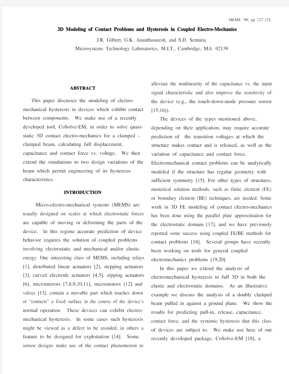
The basic features of electro-mechanical hysteresis are evident even in the simplest one dimensional model shown in Figure 1. This model is essentially a parallel-plate capacitor of area, A with a fixed ground plate, and a moving plate restrained by a linear spring of known stiffness, K. There is a rigid stop at a distance s above the ground plane (the dashed line in the figure) which corresponds to an insulating layer on the ground electrode in actual devices.

The force balance equation for this model can be written, as in equation (1), by summing together the actuating nonlinear electrostatic force, F E , and the linear restoring force due to the spring, F M .

0=F M +F E =K (g ?z )?ε0A 2z 2V

2

(1)

If we start the device at its undeformed position (z=g, in Figure 1), we can turn V on slowly (slow enough to neglect inertia), and find stable solutions for the plate position until a critical voltage, the pull-in voltage, V PI , is reached. At V PI , the 1/z 2 growth of the electrostatic force becomes dominant over the linearly increasing mechanical restoring force, and the device pulls in, stopping at z=s. In this 1D model the pull-in occurs when the plate reaches a position z=2g/3 for a

quasi-statically applied voltage. If, instead, we start with the device displaced to touch the contact surface at s, we have stable solutions at z=s, for all V>V R , the release voltage. The release voltage may be defined as the voltage at which the electrostatic force exactly balances the spring force of the pulled in plate. If V R < V PI , the system has two valid solutions over the same band of voltages, and is capable of exhibiting hysteresis. The condition V R < V PI implies that the location of the stopping plane is below 2g/3.

To simulate the same beam to be discussed below using this 1-D model, we used plate area A = 800μm 2and spring constant K= 16N/m, and so obtained the dashed hysteresis curve shown in Figure 2.

The curve shows the simulated response of the system to (slowly) ramping the voltage from 0V to above V PI and back to 0V. The pull-in and release voltages are respectively 15V and 5V for this 1D model.

s g 0

z V +-

F E

F M K

Figure 1.Sketch of the 1D model. F E is the electrostatic actuating force, F M is elastic restoring force. The fixed plate is at z=0, the moveable plate starts at z=g, and the contact surface is at z=s.

MEMS `96, pp 127-132.

The 1D model uses a single spring constant for the entire device behavior, and neglects the distributed capacitance of the deformed beam. It also neglects all fringing effects in the electrostatic analysis.

TOOLS AND METHODS FOR THE 3D PROBLEM

CoSolve-EM is a Coupled Solver for Electro-Mechanics. It finds the self-consistent solution to electro-mechanical problems using an external,boundary-based coupling between a mechanical FE solver (ABAQUS [21]) and an electrostatic BE solver (FASTCAP [22]), implementing both relaxation and SNGCR (Surface Newton - Generalized Conjugate Residual) techniques for convergence [23]. CoSolve-EM is a package that we have been developing for several years. An overview of some of its applications was given at MEMS 1995 [18]. In this paper we describe its use for 3D electromechanical contact problems with hysteresis.

CoSolve-EM can be used to find an estimate for

pull-in or release voltages in the following manner. We solve for the coupled solution of the problem at every voltage of a sequence and observe that the device has not pulled in at V i but has pulled-in at V i+1. We then estimate V i < V PI < V i+1. We can, of course choose sequences to get us any desired accuracy, at some computational cost,and CoSolve-EM does automate this process. When we plot curves of displacement vs. voltage these curves will show a line of finite slope over the jumps of pull-in or release. This line gives the bounds on the V PI or V R step.In Figure 2 the pull-in for the beam model takes place between 17.5V and 18.0V, and the curve shows a segment of finite slope there, instead of the vertical line that we expect from the underlying physics.

A BEAM UNDER ELECTROSTATIC LOAD

Consider the model problem of a beam, clamped at either end, suspended 0.7μm over a ground plane, with a contact stop at 0.1μm above the ground plane. The beam has length L = 80μm, width W = 10μm, and thickness T = 0.5μm. It has material properties, E =169GPa, ν = 0.25, and negligible residual stress.

-0.1

00.10.20.30.40.5

0.60.7-5

5

10

15

20

25

1D Model Beam

D i s p l a c e m e n t

Voltage

Figure 2.Displacement vs. voltage for the 1D model and the 3D beam. For the 3D electromechanical solver,displacement is the maximally displaced node in the model, in this case, at the center of the beam. For the 1D model, V PI =15V and V R =5V. For the beam, 17.5V

g s

L

W

T

Figure 3.Sketch of the model beam, L=80μm,W=10μm, T=0.5μm, gap g=0.7μm, and the stop s=0.1μm.The ground plane is at z=0.

MEMS `96, pp 127-132.

Figure 3 shows a sketch of such a beam A voltage is applied between the beam and the ground plane. Under such an electrostatic load the beam deflects down to the contact surface and deforms against it. The hysteresis of the displacement of the center of the beam is plotted in Figure 2. Figure 4 shows a 3D visualization of the beam deformed under 20V load.

Figure 2 shows that the 3D beam model exhibits the same qualitative hysteresis in displacement vs. voltage that we encountered in the 1D model.

The 1D and 3D models do show some differences because the 1D model ignores the deformation of the plate. Thus it overestimates the touchdown capacitance and underestimates the release voltage V R .

Design of applications such as sensors and mechanical actuators may also require the curves for capacitance vs. voltage and contact force vs. voltage.

These curves are plotted in Figure 5 and Figure 6.

Figure 4.3D view of the deformation of the beam at 20V. The view shows shading on the ground plane representing the image charge induced there. The z scale is exaggerated by a factor of 25.

2 10

-14

4 10-14

6 10-14

8 10-14

-50510152025

1D Model Beam

C a p a c i t a n c e (F )

Voltage

Figure 5.Capacitance vs. voltage for the 1D model and the 3D beam. The 1D model is overestimating the touchdown capacitance.

20406080100

1200

510152025

Beam 1D Model

C o n t a c t F o r c e (10

-6

N )Voltage

Figure 6.Contact force vs. voltage for the 1D model

and the beam.

a)

b)

c)

Figure 7.Top view of beams, (a) the basic beam. (b)wide flap (40 x 10). (c) the narrow flap (10 x 20). All in μm.

MEMS `96, pp 127-132.

3D VARIATIONS OF THE BEAM

We can now perform some design experiments on the basic beam to manipulate its V PI and V R values.Figure 7 summarizes two variants of the beam that we have simulated. Both involve attaching an asymmetric flap to the beam. In Figure 7b we sketch a beam with a wide flap (40μm x 10μm) and in Figure 7c we sketch a beam with a narrow flap (10μm x 20μm). Both variants

have the effect of lowering both the pull-in and the release voltages.

Figure 8 shows the displacement vs. increasing voltage for each of the beam variants. Figure 9 shows the displacement vs. decreasing voltage for each of the variants. In both sets of curves we can see that the design variants have shifted the pull-in and release voltages.

Figure 10 shows the capacitance vs. increasing voltage for each of the three variants. In this case the difference in V PI between the beam and the beam with narrow flap appears reduced from what was observed in Figure 8. This is explained by the fact that the narrow flap touches down before the bulk of the beam itself.Figure 11 shows the 3D image of the bottom surfaces of

the narrow flap beam at 11.5V (when the flap is just touching down). Figure 12 shows the same beam at 12.5V, after the center of the beam has been pulled down. In this example we are modeling the quasi-static version of the process of “zipping” discussed and demonstrated by several authors [4,5,6].

When we plot displacement, we are plotting the displacement of the maximally displaced point. In the case of the beam with narrow flap this point occurs at the tip of the narrow flap itself. When we plot capacitance, we are plotting a quantity more sensitive to the position of the bulk of the device. So as the device goes from its position in Figure 11 to the one in Figure

12 the reported displacement does not change (the tip is already down) but the capacitance changes considerably.

-0.1

00.10.20.30.40.5

0.60.70

5

10

15

20

Beam

Narrow Flap Wide Flap

D i s p l a c e m e n t

Voltage

Figure 8.Displacement vs. increasing voltage for the variations of the beam

-0.1

00.10.20.30.40.50.60.70

5

10

15

Beam

Narrow Flap Wide Flap

D i s p l a c e m e n t

Voltage

Figure 9.Displacement vs. decreasing voltage for each of the variations of the beam.

MEMS `96, pp 127-132.

CONCLUSION

The results reported here show that we can now perform full 3D analysis of contact electro-mechanics problems with hysteresis. Using CoSolve-EM, such problems can be solved from general meshed device descriptions, with no requirement to customize the modeler for each different type of geometry. This will enable MEMS designers to explore a wide design space of variations on interesting devices using software simulations.

ACKNOWLEDGMENTS

The CoSolve-EM package used in this paper has been developed over several years as part of the MEMCAD project at MIT. The work has been supported by DARPA contract J92-FBI-196 as well as equipment grants from Hewlett Packard and Digital Equipment. The authors would like to thank Jacob White and Rob Legtenberg for many valuable discussions and insights, as well as King Yu and Gregory Pal for their contributions to CoSolve-EM.

2 10-14

4 10-146 10-148 10-14

1 10-130

5

10

15

20

Beam

Narrow Flap Wide Flap

C a p a c i t a n c e (F )

Voltage

Figure 10.Capacitance vs.

increasing voltage for each type of beam.

Figure 11.3D view of the bottom surface of the beam with narrow flap at 11.5V, just after the initial touchdown of the flap tip. The figure is otherwise as in Figure 4.

Figure 12.3D view of the bottom surface of the beam with narrow flap at 12.5V, after the flap has pulled down the center of the beam. The figure is otherwise as in Figure 4.

MEMS `96, pp 127-132.

1 J. Drake, H. Jerman, B. Lutze, and M. Stuber, "An

Electrostatically Actuated Micro-Relay", Proc.

Transducers 95, Stockholm, paper no. 329-B10.

2 M. Yamaguchi and K. Kawamura, "Distributed

Electrostatic Microactuator", Proc. MEMS 1993, Fort Lauderdale, FL, pp. 18-23.

3 T. Akiyama and K. Shono, "A New Step Motion of

Polysilicon Microstructures", Proc. MEMS 1993, Fort Lauderdale, FL, pp. 272-277.

4 R. Legtenberg, et al., "Electrostatic Curved Electrode

Actuator", Proc. MEMS 1995, Amsterdam, pp. 37-42.

5 Branedbjerg and Gravesen, "A New Electrostatic Actuator

Providing Improved Stroke Length and Force", Proc.

MEMS 1992, Travemünde, Germany, pp. 6-11.

6 K. Sato and M. Shikida, "Electrostatic Film Actuator with

a Large Vertical Displacement", Proc. MEMS 1992,

Travemünde, Germany, pp. 1-5.

7 V. P. Jaecklin, C. Linder, and N. F. de Rooij, "Optical

Microshutters and Torsional Micromirrors for Light Modulation Arrays", Proc. MEMS 1993, Fort Lauderdale, FL, pp. 124-127.

8 J. B. Sampsell, "The Digital Micromirror Device and its

Application to Projection Displays", Proc. Transducers 93, Yokohoma, pp. 24-27.

9 H. Toshiyoshi and H. Fujita, "An Electrostatically

Operated Torsion Mirror for Optical Switching Device", Proc. Transducers 95, Stockholm, paper no. 68-B1.

10 H. Kück, W. Doleschal, A. Gehner, W. Grundke, R.

Melcher, J. Paufler, R. Seltmann, and G. Zimmer, "Deformable Micromirror Devices as Phase Modulating High Resolution Light Valves", Proc. Transducers 95, Stockholm, paper no. 69-B1.

11 M. Fischer, M. N?gele, D. Echner, C. Sch?llhorn, R.

Strobel, "Integration of Surface Micromachined Polysilicon Mirrors and a Standard CMOS Process", Proc.

Transducers 95, Stockholm, paper no. 70-B1.

12 R. Legtenberg, et al. "An Electrostatic Lower Stator Axial

Gap Wobble Motor: Design and Fabrication", Proc.

Transducers 95, Stockholm, paper no. 335-B11.

13 M. Huff, M. Mettner, T. Lober, and M. Schmidt, "A

Pressure-Balanced Electrostatically-Actuated Microvalve", Proc. IEEE Solid State Sensor and Actuator Workshop, Hilton Head, SC, 1990, pp. 123-127.14 R.B. Apte, F.S.A. Sandejas, W.C. Banyai, and D.M.

Bloom, "Deformable Grating Light Valves for High Resolution Displays", Proc. IEEE Solid State Sensor and Actuator Workshop, Hilton Head, SC,1994, pp. 1-6.

15 X. Ding, L-J. Tong, W. He, J. Hsu, and W. Ko, "Touch-

mode Silicon Capacitive Pressure Sensors", Microstructures, Sensors, and Actuators, ASME, DSC-Vol. 19. Edited by D. Cho et al., 1990, pp. 111-117.

16 L. Rosengren, J. S?deskvist, and L. Smith,

"Micromachined Sensor Structures with Linear Capacitive Response", Sensors and Actuators A, Vol. 31, pp. 200-205 (1992).

17 B.E. Artz and L.W. Cathey, "A Finite Element Method for

Determining Structural Displacements Resulting from Electrostatic Forces", Proc. IEEE Solid State Sensor and Actuator Workshop, Hilton Head, SC, 1992, pp 190-193.

18 J.R. Gilbert, R. Legtenberg, and S.D. Senturia, "3D

Coupled Electro-Mechanics for MEMS: Applications of CoSolve-EM", Proc. MEMS 1995, Amsterdam, pp. 122-127.

19 H.U. Schwarzenbach, J.G. Korvink, M. Roos, G. Sartoris,

and E. Anderheggen, "A micro electro mechanical CAD extension for SESES", J. Micromech. Microeng, Vol. 3, pp. 118-122 (1993).

20 U. Beerschwinger, et al., "Coupled Electrostatic and

Mechanical FEA of a Micromotor", JMEMS, Vol. 3, pp 162-171 (1994).

21 ABAQUS Manual, Hibbitt, Karlsson & Sorenson, Inc.

1080 Main Street, Pawtucket, RI 02860, USA.

22 K. Nabors and J. White, "FastCap: A multipole-

accelerated 3-D capacitance extraction program", IEEE Transactions on Computer-Aided Design, Vol. 10, pp.

1447-1459 (1991).

23 X. Cai, H. Yie, P. Osterberg, J. Gilbert, S. Senturia, and J.

White, "A Relaxation/Multipole-Accelerated Scheme for Self-Consistent Electromechanical Analysis of Complex 3-D Microelectromechanical Structures", Proc. Int. Conf.

on Computer-Aided Design, Santa Clara, CA, November 1993, pp. 270-274.

ADAMS常见问题

ADAMS 使用常见问题 1、ADAMS中的单位的问题 开始的时候需要为模型设置单位。在所有的预置单位系统中,时间单位就是秒,角度就是度。可设置: MMKS--设置长度为毫米,质量为千克,力为牛顿。 MKS—设置长度为米,质量为千克,力为牛顿。 CGS—设置长度为厘米,质量为克,力为达因。 IPS—设置长度为英寸,质量为斯勒格(slug),力为磅。 2、如何永久改变ADAMS的启动路径？ 在ADAMS启动后,每次更改路径很费时,我们习惯将自己的文件存在某一文件夹下;事实上,在Adams的快捷方式上右击鼠标,选属性,再在起始位置上输入您想要得路径就可以了。 3、关于ADAMS的坐标系的问题。 当第一次启动ADAMs/View时,在窗口的左下角显示了一个三视坐标轴。该坐标轴为模型数据库的全局坐标系。缺省情况下,ADAMS/View用笛卡儿坐标系作为全局坐标系。ADAMS/View将全局坐标系固定在地面上。 当创建零件时,ADAMS/View给每个零件分配一个坐标系,也就就是局部坐标系。零件的局部坐标系随着零件一起移动。局部坐标系可以方便地定义物体的位置,ADAMS/View也可返回如零件的位置——零件局部坐标系相对于全局坐标系的位移的仿真结果。局部坐标系使得对物体上的几何体与点的描述比较方便。物体坐标系不太容易理解。您可以自己建一个ｐａｒｔ,通过移动它的位置来体会。 4、关于物体的位置与方向的修改 可以有两种途径修改物体的位置与方向,一种就是修改物体的局部坐标系的位置,也就就是通过ＭＯＤＩＦＹ物体的ｐｏｓｉｔｉｏｎ属性;令一种方法就就是修改物体在局部坐标系中的位置,可以通过修改控制物体的关键点来实现。我感觉这两种方法的结果就是不同的,但就是对于仿真过程来说,物体的位置就就是质心的位置,所以对于仿真就是一样的。 5、关于ADAMS中方向的描述。 对于初学的人来说,方向的描述不太容易理解。之前我们都就是用方向余弦之类的量来描述方向的。在ADAMS中,为了求解方程就是计算的方便,使用欧拉角来描述方向。就就是用绕坐标轴转过的角度来定义。旋转的旋转轴可以自己定义,默认使用313,也就就是先绕ｚ轴,再绕ｘ轴,再绕ｚ轴。 6、Marker点与Pointer点区别 Marker:具有方向性, 大部分情況都就是伴随物件自动产生的,而 Point不具有方向性, 都就是用户自己建立的;Marker点可以用来定义构件的几何形状与方向,定义约束与运动的方向等,而Point点常用来作为参数化的参考点,若构件与参考点相连,当修改参考点的位置时,其所关联的物体也会一起移动或改变。

adams常用函数

1.step可能是最常用的: step(time,0,0,1,50)+ step(time,4,0,6,-100)+ step(tme,9,0,10,50) 函数原形STEP(A,x1,h1,x2,h2) 解释：由数组A的x值，生成区间（x1，h1）至（x2，h2）之间的阶梯曲线，返回y值的数据。 举个常用的例子。 比如STEP(time,1,0,2,100) time在adams中是个递增的变量，相当于一个数组。那么step的返回值就是随着time变化的值。 这个例子将表示在time从（1，2）的过程中，返回值将从0，100。看看例子，两个小球，一个使用step 函数设置了位移，另外一个是参考。当然，这个变化过程，adams使用了缓和的图形，从其位移图中可以看出来。step既然是个返回值，就可以使用加减法了。如上例，如果设置下面的小球的位移如下：STEP(time,1,0,2,100)+step(time,2,0,3,400)+step(time,3,0,4,-200) 2.以前用过碰撞函数，有单向和双向函数的区分，其中系统的球面等碰撞为其特例！ IMPACT (Displacement Variable, Velocity Variable, Trigger for Displacement Variable, Stiffness Coefficient, Stiffness Force Exponent, Damping Coefficient, Damping Ramp-up Distance) BISTOP (Displacement Variable, Velocity Variable, Low Trigger for Displacement Variable, High Trigger for Displacement Variable, Stiffness Coefficient, Stiffness Force Exponent, Damping Coefficient, Damping Ramp-up Distance) 3.if函数 这个函数最好不要使用，他的使用会带来突变，会使运算的时候不收敛。不过应急的时候还是可以一用。 if(time-1:1,0,if(time-2:0,-1,-1)) IF(Expression1: Expression2, Expression3, Expression4) adams要计算Expression1的值： 如果他的值小于0，则执行Expression2语句，如果Expression1的值等于0，则执行Expression3语句，如果Expression1的值大于0，则执行Expression4语句 我得if语句的意思是：如果时间小于1的时候，加速度为1，如果时间为1，加速度为0，如果时间大于1小于2，则加速度为0，如果时间大于、等于2则，加速度为-1 4. 我得一个想法 就是利用sign函数构造 比较常用的是给机构加上一个与运动方向相反的作用力等等可以先测量施加力对象的运动速度，然后利用速度的变化，插入measure到sign函数里面就可以获得与运动方向相反的作用力

ADAMS中的函数

ADAMS/View中系统提供的数学函数大致分类介绍如下。 （1）基本数学函数 ABS(x) 数字表达式x的绝对值 DIM(x1，x2) x1>x2时x1与x2之间的差值，x1<x2时返回0 EXP(x) 数字表达式x的指数值 LOG(x) 数字表达式x的自然对数值 LOG10(x) 数字表达式x的以10为底的对数值 MAG(x，y，z) 向量[x，y，z]求模 MOD(x1，x2) 数字表达式x1对另一个数字表达式x2取余数 RAND(x) 返回0到1之间的随机数 SIGN(x1，x2) 符号函数，当x2>0时返回ABS(x)，当x2<0时返回－ABS(x) SQRT(x) 数字表达式x的平方根值 （2）三角函数 SIN(x) 数字表达式x的正弦值 SINH(x) 数字表达式x的双曲正弦值 COS(x) 数字表达式x的余弦值 COSH(x) 数字表达式x的双曲余弦值 TAN(x) 数字表达式x的正切值 TANH(x) 数字表达式x的双曲正切值 ASIN(x) 数字表达式x的反正弦值 ACOS(x) 数字表达式x的反余弦值 ATAN(x) 数字表达式x的反正切值 ATAN2(x1，x2) 两个数字表达式x1，x2的四象限反正切值

（3）取整函数 INT(x) 数字表达式x取整 AINT(x) 数字表达式x向绝对值小的方向取整 ANINT(x) 数字表达式x向绝对值大的方向取整 CEIL(x) 数字表达式x向正无穷的方向取整 FLOOR(x) 数字表达式x向负无穷的方向取整 NINT(x) 最接近数字表达式x的整数值 RTOI(x) 返回数字表达式x的整数部分 位置/方向函数位置/方向函数用于根据不同输入变量计算有关位置或方向的参数。ADAMS/View中系统提供的位置/方向函数分类介绍如下。 （1）位置函数 LOC_ALONG_LINE 返回两点连线上与第一点距离为指定值的点 LOC_CYLINDRICAL 将圆柱坐标系下坐标值转化为笛卡儿坐标系下坐标值 LOC_FRAME_MIRROR 返回指定点关于指定坐标系下平面的对称点 LOC_GLOBAL 返回参考坐标系下的点在全局坐标系下的坐标值 LOC_INLINE 将一个参考坐标系下的坐标值转化为另一参考坐标系下的坐标值并归一化 LOC_LOC 将一个参考坐标系下的坐标值转化为另一参考坐标系下的坐标值

ADAMS部分常用函数的说明

ADAMS常用函数的说明 一、几个常用函数的说明 1、 STEP函数 格式：STEP (x, x0, h0, x1, h1) 参数说明： x ―自变量，可以是时间或时间的任一函数 x0 ―自变量的STEP函数开始值，可以是常数或函数表达式或设计变量； x1 ―自变量的STEP函数结束值，可以是常数、函数表达式或设计变量； h0 ― STEP函数的初始值，可以是常数、设计变量或其它函数表达式； h1 ― STEP函数的最终值，可以是常数、设计变量或其它函数表达式。 2、 IF函数 格式：IF(表达式1: 表达式2, 表达式3, 表达式4) 参数说明： 表达式1－ADAMS的评估表达式； 表达式2－如果的Expression1值小于0，IF函数返回的Expression2值； 表达式3－如果表达式1的值等于0，IF函数返回表达式3的值； 表达式4－如果表达式1的值大于0，IF函数返回表达式4的值；

例如：函数IF(time-2.5:0,0.5,1) 结果：0.0 if time < 2.5 0.5 if time = 2.5 1.0 if time > 2.5 3、AKISPL函数 格式：AKISPL (First Independent Variable, Second Independent Variable，Spline Name, Derivati ve Order) 参数说明： First Independent Variable ——spline中的第一个自变量 Second Independent Variable(可选) ——spline中的第二自变量 Spline Name ——数据单元spline的名称 Derivative Order(可选) ——插值点的微分阶数，一般用0就可以了 例如： function = AKISPL(DX(marker_1, marker_2), 0, spline_1) spline_1用下表中的离散数据定义：

adams常见函数总结

ADAMS常用函数总结 在使用adams的过程中，由于函数比较多，大概有11种之多，如1、Displacement Fu nction 2、Velocity Functions 3、Acceleration Functions 4、Contact Functions 5、Spline Functions 6、Force in Object Functions 7、Resultant Force Functi ons 8、Math Functions 9、Data Element Access 10、User-Written Subroutine Invocation 11、Constants & Variables。 在adams中也有帮助文档，但是对于初学者来说还是有一定的难度的，基于这种情况我总结了一下几种常用的函数，希望能够起到抛砖引玉的作用！ 1、STEP函数 格式：STEP (x, x0, h0, x1, h1) 参数说明： x―自变量，可以是时间或时间的任一函数 x0 ―自变量的STEP函数开始值，可以是常数或函数表达式或设计变量； x1 ―自变量的STEP函数结束值，可以是常数、函数表达式或设计变量 h0 ―STEP函数的初始值，可以是常数、设计变量或其它函数表达式 h1 ―STEP函数的最终值，可以是常数、设计变量或其它函数表达式 2、IF函数 格式：IF(表达式1: 表达式2, 表达式3, 表达式4) 参数说明： 表达式1－ADAMS的评估表达式； 表达式2－如果的Expression1值小于0，IF函数返回的Expression2值； 表达式3－如果表达式1的值等于0，IF函数返回表达式3的值； 表达式4－如果表达式1的值大于0，IF函数返回表达式4的值； 例如：函数IF(time-2.5:0,0.5,1) 结果：0.0 if time < 2.5 0.5 if time = 2.5 1.0 if time > 2.5 3、AKISPL函数 格式：AKISPL (First Independent Variable, Second Independent Variable，Spline Name, Derivative Order) 参数说明： First Independent Variable——spline中的第一个自变量 Second Independent Variable (可选) ——spline中的第二自变量Spline Name——数据单元spline的名称 Derivative Order (可选) ——插值点的微分阶数，一般用0就可以function = AKISPL(DX(marker_1, marker_2, marker_2), 0, spline_1) spline_1用下表中的离散数据定义 自变量x 函数值y -4.0 -3.6 -3.0 -2.5 -2.0 -1.2

adams中函数用法

Adams常用函数 step可能是最常用的: step(time,0,0,1,50)+ step(time,4,0,6,-100)+ step(tme,9,0,10,50) 函数原形STEP(A,x1,h1,x2,h2) 解释：由数组A的x值，生成区间（x1，h1）至（x2，h2）之间的阶梯曲线，返回y值的数据。 举个常用的例子。 比如STEP(time,1,0,2,100) time在adams中是个递增的变量，相当于一个数组。那么step的返回值就是随着time变化的值。 这个例子将表示在time从（1，2）的过程中，返回值将从0，100。看看例子，两个小球，一个使用step 函数设置了位移，另外一个是参考。当然，这个变化过程，adams使用了缓和的图形，从其位移图中可以看出来。step既然是个返回值，就可以使用加减法了。如上例，如果设置下面的小球的位移如下：STEP(time,1,0,2,100)+step(time,2,0,3,400)+step(time,3,0,4,-200) 1.以前用过碰撞函数，有单向和双向函数的区分，其中系统的球面等碰撞为其特例！ IMPACT (Displacement Variable, Veloci t y Variable, Trigger for Displacement Variable, Stiffness Coefficient, Stiffness Force Exponent, Damping Coefficient, Damping Ramp-up Distance) BISTOP (Displacement Variable, Velocity Variable, Low Trigger for Displacement Variable, High Trigger for Displacement Variable, Stiffness Coefficient, Stiffness Force Exponent, Damping Coefficient, Damping Ramp-up Distance) 2.if函数 这个函数最好不要使用，他的使用会带来突变，会使运算的时候不收敛。不过应急的时候还是可以一用。 if(time-1:1,0,if(time-2:0,-1,-1)) IF(Expression1: Expression2, Expression3, Expression4) adams要计算Expression1的值： 如果他的值小于0，则执行Expression2语句，如果Expression1的值等于0，则执行Expression3语句，如果Expression1的值大于0，则执行Expression4语句 我得if语句的意思是：如果时间小于1的时候，加速度为1，如果时间为1，加速度为0，如果时间大于1小于2，则加速度为0，如果时间大于、等于2则，加速度为-1 4. 我得一个想法 就是利用sign函数构造 比较常用的是给机构加上一个与运动方向相反的作用力等等可以先测量施加力对象的运动速度，然后利用速度的变化，插入measure到sign函数里面就可以获得与运动方向相反的作用力

adams初级设置教程

1、ADAMS中的单位的问题 开始的时候需要为模型设置单位。在所有的预置单位系统中,时间单位是秒,角度是度。可设置: MMKS--设置长度为千米,质量为千克,力为牛顿。 MKS—设置长度为米,质量为千克,力为牛顿。 CGS—设置长度为厘米,质量为克,力为达因。 IPS—设置长度为英寸,质量为斯勒格(slug),力为磅。 2、如何永久改变ADAMS的启动路径？ 在ADAMS启动后，每次更改路径很费时，我们习惯将自己的文件存在某一文件夹下；事实上，在Adams的快捷方式上右击鼠标，选属性，再在起始位置上输入你想要得路径就可以了。 3、关于ADAMS的坐标系的问题。 当第一次启动ADAMs/View时,在窗口的左下角显示了一个三视坐标轴。该坐标轴为模型数据库的全局坐标系。缺省情况下,ADAMS/View用笛卡儿坐标系作为全局坐标系。ADAMS/View将全局坐标系固定在地面上。 当创建零件时,ADAMS/View给每个零件分配一个坐标系,也就是局部坐标系。零件的局部坐标系随着零件一起移动。局部坐标系可以方便地定义物体的位 置,ADAMS/View也可返回如零件的位置——零件局部坐标系相对于全局坐标系 的位移的仿真结果。局部坐标系使得对物体上的几何体和点的描述比较方便。物体坐标系不太容易理解。你可以自己建一个ｐａｒｔ，通过移动它的位置来体会。 4、关于物体的位置和方向的修改 可以有两种途径修改物体的位置和方向，一种是修改物体的局部坐标系的位置，也就是通过ＭＯＤＩＦＹ物体的ｐｏｓｉｔｉｏｎ属性；令一种方法就是修改物体在局部坐标系中的位置，可以通过修改控制物体的关键点来实现。我感觉这两种方法的结果是不同的，但是对于仿真过程来说，物体的位置就是质心的位置，所以对于仿真是一样的。

《交通规划》课程教学大纲

《交通规划》课程教学大纲 课程编号：E13D3330 课程中文名称：交通规划 课程英文名称：Transportation Planning 开课学期：秋季 学分/学时：2学分/32学时 先修课程：管理运筹学，概率与数理统计，交通工程学 建议后续课程：城市规划，交通管理与控制 适用专业/开课对象：交通运输类专业/3年级本科生 团队负责人：唐铁桥责任教授：执笔人：唐铁桥核准院长： 一、课程的性质、目的和任务 本课程授课对象为交通工程专业本科生，是该专业学生的必修专业课。通过本课程的学习，应该掌握交通规划的基础知识、常用方法与模型。课程具体内容包括：交通规划问题分析的一般方法，建模理论，交通规划过程与发展历史，交通调查、出行产生、分布、方式划分与交通分配的理论与技术实践，交通网络平衡与网络设计理论等，从而在交通规划与政策方面掌握宽广的知识和实际的操作技能。 本课程是一间理论和实践意义均很强的课程，课堂讲授要尽量做到理论联系实际，模型及其求解尽量结合实例，深入浅出，使学生掌握将交通规划模型应用于实际的基本方法。此外，考虑到西方在该领域内的研究水平，讲授时要多参考国外相关研究成果，多介绍专业术语的英文表达方法以及相关外文刊物。课程主要培养学生交通规划的基本知识、能力和技能。 二、课程内容、基本要求及学时分配 各章内容、要点、学时分配。适当详细，每章有一段描述。 第一章绪论（2学时） 1. 交通规划的基本概念、分类、内容、过程、发展历史、及研究展望。 2. 交通规划的基本概念、重要性、内容、过程、发展历史以及交通规划中存在的问题等。

第二章交通调查与数据分析（4学时） 1. 交通调查的概要、目的、作用和内容等；流量、密度和速度调查；交通延误和OD调查；交通调查抽样；交通调查新技术。 2. 交通中的基本概念，交通流量、速度和密度的调查方法，调查问卷设计与实施，调查抽样，调查结果的统计处理等。 第三章交通需求预测（4学时） 1. 交通发生与吸引的概念；出行率调查；发生与吸引交通量的预测；生成交通量预测、发生与吸引交通量预测。 2. 掌握交通分布的概念；分布交通量预测；分布交通量的概念，增长系数法及其算法。 3. 交通方式划分的概念；交通方式划分过程；交通方式划分模型。 第四章道路交通网络分析（4学时） 1. 交通网络计算机表示方法、邻接矩阵等 2. 交通阻抗函数、交叉口延误等。 第五章城市综合交通规划（2学时） 1. 综合交通规划的任务、内容；城市发展战略规划的基本内容和步骤 2. 城市中长期交通体系规划的内容、目标以及城市近期治理规划的目标与内容 第六章城市道路网规划（2学时） 城市路网、交叉口、横断面规划及评价方法。 第七章城市公共交通规划（2学时） 城市公共交通规划目标任务、规划方法、原则及技术指标。 第八章停车设施规划（2学时） 停车差设施规划目标、流程、方法和原则。 第九章城市交通管理规划（2学时） 城市交通管理规划目标、管理模式和管理策略。 第十章公路网规划（2学时） 公路网交通调查与需求预测、方案设计与优化。 第十一章交通规划的综合评价方法（2学时） 1. 交通综合评价的地位、作用及评价流程和指标。 2. 几种常见的评价方法。 第十二章案例教学（2学时）

adams函数

adams 函数 ADAMS/View 运行函数及ADAMS/Solver 函数 2008-04-18 04:54 3 ADAMS/View 运行函数及ADAMS/Solver 函数 ADAMS/View 运行函数能够表明定义系统行为的仿真状态间的数学关系。在ADAMS/ View 中将这些运行函数与其他不同元素一同创建各种系统变量，这些函数大多数都以施加 力和产生运动为目的。之后在仿真中进行解算时，ADAMS/ Solver 会用到这些变量函数并 进行计算更新，在仿真过程中这些系统状态会发生改变，如随时间的改变而改变、随零件 的移动而改变、施加的力以不同方式改变等。 3.1 位移函数 （1）线位移函数 DX 返回位移矢量在坐标系X 轴方向的分量 DY 返回位移矢量在坐标系Y 轴方向的分量 DZ 返回位移矢量在坐标系Z 轴方向的分量 DM 返回位移距离 （2）角位移函数 AX 返回一指定标架绕另一标架X 轴旋转的角度 AY 返回一指定标架绕另一标架Y 轴旋转的角度 AZ 返回一指定标架绕另一标架Z 轴旋转的角度 （3）按313 顺序的角位移 PSI 按照313 旋转顺序,返回指定坐标系相对于参考坐标系的第一旋转角度 THETA 按照313 旋转顺序,返回指定坐标系相对于参考坐标系的第二旋转角度 PHI 按照313 旋转系列,返回指定坐标系相对于参考坐标系的第三旋转角度 （4）按照321 顺序的角位移 YAW 按照321 旋转顺序,返回指定坐标系相对于参考坐标系的第一旋转角度 PITCH 按照321 旋转顺序,返回指定坐标系相对于参考坐标系的第二旋转角度的相 反数 ROLL 按照321 旋转顺序,返回指定坐标系相对于参考坐标系的第三旋转角度 3.2 速度函数 （1）线速度函数 VX 返回两标架相对于指定坐标系的速度矢量差在X 轴的分量 VY 返回两标架相对于指定坐标系的速度矢量差在Y 轴的分量 VZ 返回两标架相对于指定坐标系的速度矢量差在Z 轴的分量 VM 返回两标架相对于指定坐标系的速度矢量差的幅值 VR 返回两标架的径向相对速度 （2）角速度函数 WX 返回两标架的角速度矢量差在X 轴的分量

ADAMS函数使用精华

样条差值函数 Akima Fitting Method(AKISPL) 定义:由曲线或者曲面返回曲线的导数或者曲线的拟合值。通过Akima样条曲线拟合方法,使用一系列离散点来拟合曲线。 格式:AKISPL(第一独立变量,第二独立变量,样条函数名,求导阶数) 自变量:第一独立变量(必须)--代表样条中第一独立变量的实数变量。 第二独立变量(必须)-- 代表样条中第二独立变量的实数变量。 样条函数名字(必须)—已存在的数据样条实体的名字,定义了用作拟合的一系列离散点。 求导阶树(可选)—在求离散点时用作求导的阶树。 其合法值为: *0—返回曲线坐标值。 *1—返回一阶导数值。 *2—返回二阶导数值。 注意:当拟合曲面时,不必指明Derivative Order(求导阶数)。 例子:某样条曲线,spline_1,其定义的离散点如下表所示。使用Akima样条拟合方法将这些离散点生成拟合函数。 既然样条曲线定义的是曲线而不是曲面, 因此, 将Second Independent Variable(第二独立变量)设置为零。 在下列例子中,给出了独立变量的值和数据,AKISPL返回拟合值: f = AKISPL(DX(marker_1, marker_2, marker_2), 0, spline_1) 由以上拟合点生成的样条曲线如下图所示:

CURVE 定义:CURVE 函数定义了一条B 样条曲线或者以CURVE 声明创建的用户自定义曲线。 格式: CURVE (alpha, iord, comp, id) 自变量:alpha —确定独立变量α的值的实变量,其中CURVE 函数计算曲线。如果曲线是以CURVE 计算的B 样条曲 线, α的取值范围为11-≤≤α。如果曲线是通过CURSUB 计算得出,alpha 的去值范围为MAXPAR MINPAR ≤≤α。 Iord —定义CURVE 函数中求导阶树的整数值。其合法值为 *0—返回曲线坐标。 *1—返回一阶偏导。 *2—返回二阶偏导。 Comp —定义CURVE 函数中分量的整数变量。其合法值为: *1—返回x 坐标值或者其导数值。 *2—返回y 坐标值或者其导数值。 *3—返回z 坐标值或者其导数值。 自变量iord 和icomp 组合在一起可以让你获得下面九个值的任何一个: Id —定义CURVE 中标志符的整数变量。

adams个别问题总结

Adams个别问题总结 1、如何永久改变ADAMS的启动路径 在ADAMS启动后，每次更改路径很费时，我们习惯将自己的文件存在某一文件夹下；事实上，在Adams的快捷方式上右击鼠标，选属性，再在起始位置上输入你想要得路径就可以了。 2、ADAMS中的单位的问题 开始的时候需要为模型设置单位。在所有的预置单位系统中,时间单位是秒,角度是度。可设置: MMKS--设置长度为千米,质量为千克,力为牛顿。 MKS—设置长度为米,质量为千克,力为牛顿。 CGS—设置长度为厘米,质量为克,力为达因。 IPS—设置长度为英寸,质量为斯勒格(slug),力为磅。 在模型运行的过程中也可以改变单位系统的设定。还可以在文本框中使用自己的单位，比如默认的角度单位度时可以使用Ｒ表示弧度。我感觉在ADAMS 内部好像是把所有的带单位的输入量都转换成统一的单位了。 3、关于ADAMS的坐标系的问题。 当第一次启动ADAMs/View时,在窗口的左下角显示了一个三视坐标轴。该坐标轴为模型数据库的全局坐标系。缺省情况下,ADAMS/View用笛卡儿坐标系作为全局坐标系。ADAMS/View将全局坐标系固定在地面上。 当创建零件时,ADAMS/View给每个零件分配一个坐标系,也就是局部坐标系。零件的局部坐标系随着零件一起移动。局部坐标系可以方便地定义物体的位置,ADAMS/View也可返回如零件的位置——零件局部坐标系相对于全局坐标系的位移的仿真结果。局部坐标系使得对物体上的几何体和点的描述比较方便。物 体坐标系不太容易理解。你可以自己建一个part，通过移动它的位置来体会。4、关于物体的位置和方向的修改 可以有两种途径修改物体的位置和方向，一种是修改物体的局部坐标系的位置，也就是通过modify物体的position属性；令一种方法就是修改物体在局部坐标系中的位置，可以通过修改控制物体的关键点来实现。我感觉这两种方法的结果是不同的，但是对于仿真过程来说，物体的位置就是质心的位置，所以对于仿真是一样的。 5、关于ADAMS中方向的描述。 对于初学的人来说，方向的描述不太容易理解。之前我们都是用方向余弦之类的量来描述方向的。在ADAMS中，为了求解方程是计算的方便，使用欧拉角来描述方向。就是用绕坐标轴转过的角度来定义。旋转的旋转轴可以自己定义，默认使用313，也就是先绕ｚ轴，再绕ｘ轴，再绕ｚ轴。 6、Marker点与Pointer点区别

(完整版)ADAMS常用函数的说明

一、几个常用函数的说明 1、 STEP函数 格式：STEP (x, x0, h0, x1, h1) 参数说明： x ―自变量，可以是时间或时间的任一函数 x0 ―自变量的STEP函数开始值，可以是常数或函数表达式或设计变量； x1 ―自变量的STEP函数结束值，可以是常数、函数表达式或设计变量； h0 ― STEP函数的初始值，可以是常数、设计变量或其它函数表达式； h1 ― STEP函数的最终值，可以是常数、设计变量或其它函数表达式。 2、 IF函数 格式：IF(表达式1: 表达式2, 表达式3, 表达式4) 参数说明： 表达式1－ADAMS的评估表达式； 表达式2－如果的Expression1值小于0，IF函数返回的Expression2值； 表达式3－如果表达式1的值等于0，IF函数返回表达式3的值； 表达式4－如果表达式1的值大于0，IF函数返回表达式4的值； 例如：函数IF(time-2.5:0,0.5,1)

结果：0.0 if time < 2.5 0.5 if time = 2.5 1.0 if time > 2.5 3、AKISPL函数 格式：AKISPL (First Independent Variable, Second Independent Variable，Spline Name, Derivati ve Order) 参数说明： First Independent Variable ——spline中的第一个自变量 Second Independent Variable(可选) ——spline中的第二自变量 Spline Name ——数据单元spline的名称 Derivative Order(可选) ——插值点的微分阶数，一般用0就可以了 例如： function = AKISPL(DX(marker_1, marker_2), 0, spline_1) spline_1用下表中的离散数据定义：

ADAMS软件中IMPACT函数参数的确定(精)

3.3.3 ADAMS 软件中IMPACT 函数参数的确定 (1) 碰撞函数中的非线性弹簧参数的确定 在使用ADAMS 碰撞函数中，确定碰撞力大小n F 主要由等效刚度k 以及幂指数q 两个参数确定。为了合理的确定等效刚度以及幂指数，通常使用Hertz 弹性碰撞模型来计算出正确的k 与q 。Hertz 弹性碰撞模型如下： 图3-3 弹性碰撞示意图 如图3-3所示，设某一半径为R 的圆球体A 以速度v 飞向平面B ，则该过程 分为以下三个主要过程： 当碰撞发生时，物体A 与物体B 之间有力的作用，其中在碰撞时因为碰撞产生了弹性力n F 同时物体A 也发生了一定的变形δ，Hertz 模型指出n F 与δ满足如下关系： 1 23 2916n F ER δ??= ? ?? (3-14) 其中： 12111R R R =+（R1,R2分别为碰撞点处两物体的曲率半径） 2 2 1212 (1)(1)1E E E μμ--=+（E1,E2分别为两物体的材料弹性模量, 1μ , 2μ分别为两物体的材料泊松比） 由式(3-14)我们可知 2 3 216*9n RE F δ??= ??? (3-15) 故而可以确定 2169RE k ??= ??? (2) 碰撞函数中的阻尼参数max c 的确定 v B ' B （a ）碰撞前 （c ）碰撞后 （b ）碰撞

式(3-12)可以写成 n n F k D δδ =+ (3-16) 其中D 为该式中的阻尼参数，δ 为两物体接触时的相对移动速度。Hund 与 Grossley [83]曾提出确定D 的方法： n D μδ= (3-17) 在式(3-17)中μ被称为滞后阻尼因子。在碰撞非线性弹簧阻尼模型中，碰撞过程会导致能量的损失，这是由碰撞的阻尼项造成的。图3-4表示在碰撞过程中碰撞 力的变化： 在该图中()t -表示开始碰撞前的那一时刻， ()m t 表示碰撞达到最大穿透量的那一时刻，()t +表示开始碰撞结束后两物体分离的那一时刻。在式(3-17)中阻尼系数D 或 滞后阻尼因子μ需要确定。应用经典的冲量定理与能量守恒原理可以确定以上两个变量。 根据能量守恒定理可知在碰撞前与碰撞后两物体的动能损失可以用恢复系 数e 与两物体间的相对速度()δ - 来表示 其中()()()i j V V δ---=- (()i V -表示物体i 碰撞接触前的速度，()j V - 表示物体j 碰撞接触前的速度) 图3-4 碰撞力的变化

ADAMS函数使用精华

ADAMS的函数种类比较多： 1、Displacement Functions 2、Velocity Functions 3、Acceleration Functions 4、Contact Functions 5、Spline Functions 6、Force in Object Functions 7、Resultant Force Functions 8、Math Functions 9、Data Element Access 10、User-Written Subroutine Invocation 11、Constants&Variables 虽然在ADAMS的帮助文档有些说明， 但实际使用时初学者可能往往遇到困难. 一、几个常用函数的说明 1、STEP函数 格式：STEP(x,x0,h0,x1,h1) 参数说明： x―自变量，可以是时间或时间的任一函数 x0―自变量的STEP函数开始值，可以是常数或函数表达式或设计变量； x1―自变量的STEP函数结束值，可以是常数、函数表达式或设计变量 h0―STEP函数的初始值，可以是常数、设计变量或其它函数表达式 h1―STEP函数的最终值，可以是常数、设计变量或其它函数表达式 2、IF函数 格式：IF(表达式1:表达式2,表达式3,表达式4) 参数说明： 表达式1－ADAMS的评估表达式； 表达式2－如果的Expression1值小于0，IF函数返回的Expression2值； 表达式3－如果表达式1的值等于0，IF函数返回表达式3的值； 表达式4－如果表达式1的值大于0，IF函数返回表达式4的值； 例如：函数IF(time-2.5:0,0.5,1) 结果：0.0if time<2.5 0.5if time=2.5 1.0if time> 2.5 3、AKISPL函数 格式：AKISPL(First Independent Variable,Second Independent Variable，Spline Name,

ADAMS中step函数的用法

step函数的两种表示方法 相信大家对step的用法已经是相当的熟练了，在这里我只是想把自己对step的理解总结一下，希望能对大家有所帮助。 首先简要介绍下step的形式及其各个参数的物理含义： 格式：STEP (x, x0, h0, x1, h1) 参数说明： x ―自变量，可以是时间或时间的任一函数 x0 ―自变量的STEP函数开始值，可以是常数或函数表达式或设计变量； x1 ―自变量的STEP函数结束值，可以是常数、函数表达式或设计变量 h0 ― STEP函数的初始值，可以是常数、设计变量或其它函数表达式 h1 ― STEP函数的最终值，可以是常数、设计变量或其它函数表达式 而在实际的运用过程中，它有两种表示方法，一种是嵌入式： STEP (x, x0, h0, x1, （STEP (x, x1, h1, x2, （STEP (x, x2, h2, x3, h2) ））））（当然你可以嵌套更多的） 另一种就是增量式： STEP (x, x0, h0, x1, h1)+ STEP (x, x1, h2, x2, h3)+ STEP (x, x2, h4, x3, h5)+ …… 我常用的是后者，下面就举例（附件请参考step.cmd文件）说明下他们的区别。其实他们都可以表示同一种你所需要的曲线，如下所示曲线： 用嵌入式可表示为： step(time,0,0d,3, (step(time,3,0d,5, (step(time,5,5d,8, (step(time,8,5d,10, (step(time,10,0d,12,0d))))))))) 用增量式表示为： step(time,3,0,5,5)+ step(time,5,0,8,0)+ step(time,8,0,10,-5)

Adams常用函数介绍

常数函数 常用的常数函数（constant）：PI圆周率；RTOD弧度转化为度数时的乘积系数，值为180/PI；DTOR度数转化为弧度时的乘积系数，值为PI/ 180。 运动副的驱动函数 function：30.0d*time，type：displacement和function：30.0d，type：velocity 作用是一样的，它们都表示角速度为30.0。同样，function：30.0d*time，type：velocity和function：30.0d，type：acceleration作用也是一样的，它们都表示角加速度为30.0。一般应优先使用function：30.0d，type：velocity这种表示法，它更简单，更便于理解。 function：5，type：acceleration，表示物体的加速度为常数5；function：STEP( time , 0 , 0 , 5 , 25 )，type：velocity，表示物体的速度从（0，0）变化为（5，25），物体的加速度并不是一个常数，加速度的图形是一条先增后减的弧线。在定义驱动函数时，如果已知物体的加速度为5，则应采用第一个表达式；如果不知道加速度的变化规律，只知道速度由0，0）变化为（5，25），则应采用第二个表达式。 d是degree度数的简写，在此d并不是单位，而是用来区分滑移运动和旋转运动，代表旋转。旋转副的驱动函数中函数值后必须加d，如STEP( time , 0 , 0d , 3 , 300d )，而滑移副的驱动函数中函数值后不能加d。则直接数字，默认单位。 常用的驱动函数STEP 格式：STEP (x, x0, h0, x1, h1) 参数说明： x ―自变量，可以是时间或时间的任一函数； x0 ―自变量的STEP函数开始值； x1 ―自变量的STEP函数结束值； h0 ―当前时间点相对于上一时间点的函数值增量； h1 ―当前时间点相对于上一时间点的函数值增量。 例：旋转运动副的驱动函数（function）为STEP( time , 0 , 0d , 3 , 300d )+STEP( time , 3 , 0d , 6 , 0d )+STEP( time , 6 , 0d , 9 , -300d )，函数值（type）为velocity，STEP( time , 3 , 0d , 6 , 0d )可省略。驱动函数表示物体在0-3s做加速运动，速度由0 d变为300d，物体在3-6s做匀速运动，速度不变，物体在6-9s

Adams中的命令

ADAMS常用函数总结！ 在使用adams的过程中，由于函数比较多，大概有11种之多，如 1、Displacement Function 2、Velocity Functions 3、 Acceleration Functions 4、 Contact Functions 5、 Spline Functions 6、 Force in Object Functions 7、Resultant Force Functions 8、 Math Functions 9、 Data Element Access 10、User-Written Subroutine Invocation 11、Constants & Variables。 在adams中也有帮助文档，但是对于初学者来说还是有一定的难度的，基于这种情况我总结了一下几种常用的函数，希望能够起到抛砖引玉的作用！ 1、 STEP函数 格式：STEP (x, x0, h0, x1, h1) 参数说明： x ―自变量，可以是时间或时间的任一函数 x0 ―自变量的STEP函数开始值，可以是常数或函数表达式或设计变量； x1 ―自变量的STEP函数结束值，可以是常数、函数表达式或设计变量 h0 ― STEP函数的初始值，可以是常数、设计变量或其它函数表达式 h1 ― STEP函数的最终值，可以是常数、设计变量或其它函数表达式 2、 IF函数 格式：IF(表达式1: 表达式2, 表达式3, 表达式4) 参数说明： 表达式1－ADAMS的评估表达式； 表达式2－如果的Expression1值小于0，IF函数返回的Expression2值； 表达式3－如果表达式1的值等于0，IF函数返回表达式3的值； 表达式4－如果表达式1的值大于0，IF函数返回表达式4的值； 例如：函数 IF(time-2.5:0,0.5,1) 结果： 0.0 if time < 2.5 0.5 if time = 2.5 1.0 if time > 2.5 MSC.ADAMS 中IF语的写法和含义 □基本粒子发表于 2005-7-6 20:52:00 IF 语句的形式是这样的 IF（表达式1：表达式2，表达式3，表达式4） 如果表达式1的值小于0 执行表达式2 如果表达式1的值等于0 执行表达式3 如果表达式1的值大于0 执行表达式4 所以你的函数可以写为 IF（time-8:你的表达式，你的表达式，0）就可以了