Gong CVPR 2013 - Learning Binary Codes for High-Dimensional Data Using Bilinear Projections

第28卷㊀第5期2023年10月㊀哈尔滨理工大学学报JOURNAL OF HARBIN UNIVERSITY OF SCIENCE AND TECHNOLOGY㊀Vol.28No.5Oct.2023㊀㊀㊀㊀㊀㊀㊀㊀㊀㊀空间通道双重注意力道路场景语义分割王小玉,㊀林㊀鹏(哈尔滨理工大学计算机科学与技术学院,哈尔滨150080)摘㊀要:无人驾驶领域的一个重要问题就是在低功耗移动电子设备上怎样运行实时高精度语义分割模型㊂由于现有语义分割算法参数量过多㊁内存占用巨大导致很难满足无人驾驶等现实应用的问题,并且在影响语义分割模型的精度和推理速度的众多因素中,空间信息和上下文特征尤为重要,并且很难同时兼顾㊂针对该问题提出采用不完整的ResNet18作为骨干网络,ResNet18是一个轻量级的模型,参数量较少,占用内存不大;同时采用双边语义分割模型的技术,在两条路径上添加通道空间双重注意力机制,来获取更多的上下文信息和空间信息的想法㊂另外还采用了精炼上下文信息的注意力优化模块,和融合两条路径输出的融合模块,添加的模块对于参数量和内存的影响很小,可以即插即用㊂以Cityscapes 和CamVid 为数据集㊂在Citycapes 上,mIoU 达到77.3%;在CamVid 上,mIoU 达到66.5%㊂输入图像分辨率为1024ˑ2048时,推理时间为37.9ms ㊂关键词:无人驾驶;实时语义分割;深度学习;注意力机制;深度可分离卷积DOI :10.15938/j.jhust.2023.05.013中图分类号:TP391.41文献标志码:A文章编号:1007-2683(2023)05-0103-07Semantic Segmentation of Unmanned Driving SceneBased on Spatial Channel Dual AttentionWANG Xiaoyu,㊀LIN Peng(Harbin University of Scienceand Technology,Computer Scienceand Technology,Harbin 150080,China)Abstract :An important issue in the field of unmanned driving is how to run real-time high-precision semantic segmentation modelson low-power mobile electronic devices.Existing semantic segmentation algorithms have too many parameters and huge memory usage,which makes it difficult to meet the problems of real-world applications such as unmanned driving.However,among the many factors that affect the accuracy and speed of the semantic segmentation model,spatial information and contextual features are particularly important,and it is difficult to take into account both.In response to this problem,it is proposed to use the incomplete ResNet18as the backbone network,design a bilateral semantic segmentation model,and add a channel space dual attention model to the two paths to obtain more contextual and spatial information.In addition,the attention optimization module that refines the context information and the fusion module that integrates the output of the two paths are also used.Take Cityscapes and CamVid as data sets.On Citycapes,mIoU reached 77.3%;on CamVid,mIoU reached 66.5%.When the input image resolution is 1024ˑ2048,the segmentation speed is 37.9ms.Keywords :driverless technology;real-time semantic segmentation;deep learning;attention mechanism;depth separable convolu-tion㊀㊀㊀㊀㊀㊀㊀㊀㊀㊀㊀㊀㊀㊀㊀㊀㊀㊀㊀㊀㊀㊀㊀㊀㊀㊀㊀㊀㊀㊀㊀㊀㊀㊀㊀㊀㊀㊀㊀㊀㊀㊀㊀㊀㊀㊀㊀㊀㊀㊀㊀㊀㊀㊀㊀㊀㊀㊀㊀㊀㊀㊀㊀㊀㊀㊀㊀㊀㊀㊀㊀㊀㊀㊀㊀㊀㊀㊀㊀㊀㊀㊀㊀㊀㊀㊀㊀㊀㊀㊀㊀㊀㊀㊀㊀㊀㊀㊀㊀㊀㊀㊀㊀㊀㊀㊀收稿日期:2022-04-04基金项目:国家自然科学基金(61772160);黑龙江省教育厅科学技术研究项目(12541177).作者简介:林㊀鹏(1997 ),男,硕士研究生.通信作者:王小玉(1971 ),女,教授,硕士研究生导师,E-mail:wangxiaoyu@.0㊀引㊀言随着人工智能与汽车交通的结合, 自动驾驶热潮被掀起,如何准确㊁快速地检测路况㊁路标等信息成为目前研究的热点目标[1]㊂许多研究人员逐渐将注意力转向了对道路场景的理解㊂主要领域之一是道路场景的语义分割[2]㊂基于深度学习的图像语义分割作为计算机视觉中的一项基本任务,旨在估计给定输入图像中所有像素的类别标签,并呈现出不同颜色区域掩模的分割结果㊂2014年,文[2]提出的全卷积神经网络(FCN),被誉为深度卷积神经网络的奠基之作,标志着分割领域正式进入全新的发展时期㊂与之前所有图像语义分割算法最大的不同在于,FCN用卷积层代替分类模型中全部的全连接层,学习像素到像素的映射㊂并且,提出了在上采样阶段联合不同池化层的结果,来优化最终输出的方法[2]㊂目前很多的优秀的基于深度学习的图像语义分割算法都是基于FCN的思想实现的[3]㊂2015年,剑桥大学在FCN的基础上,实现了突破,提出了SegNet模型[3]㊂从那时起,更多的语义分割算法被开发出来,并且分割的准确性一直在提高,如deeplab系列[4],多路级联模型(refinenet)[4]和PSPNet等[5]㊂近年来,深度学习在图像语义分割方面有了很大的进步㊂在自动驾驶等领域有着很大的应用潜力㊂但是算法模型大多关注对图像分割准确率的提升,其计算成本和内存占用较高,模型的实时性得不到保证[6]㊂在许多实际应用中,对于模型的实时性也有很高的要求㊂根据这一需求,目前最常用的ENet,MobileNet系列也随即被提出[7]㊂实时进行语义信息分割技术逐渐分化一个新的领域㊂在实时语义分割的任务中,为了提高推理速度,有的模型采取缩小图片尺寸的操作,有的采取删减特征图通道的操作,但是这些操作都会丢失一些空间信息[7]㊂这是因为初始图像经历了多次卷积和池化,最终导致初始图片被模型加载后,特征图的分辨率由大变小㊂对于分割任务来说,获取丰富的上下文信息和空间信息㊁高分辨率的特征㊁深层特征的语义信息,可以更好地提高模型的分割精度[8]㊂近年来,在实时语义信息分割算法中,双边分割网络算法(BiSeNet)在语义分割任务上获得了瞩目的成绩[9]㊂本文在BiSeNet的基础上,上下文路径以轻量化模型ResNet18作为骨干网络㊂引入两个空间通道双重注意力机制CBAMT和CSSE模块㊂通过在上下文路径的轻量型特征提取网络引入CBAMT模块,从空间和通道两个维度来判断应该学习什么特征[10]㊂然后使用注意力优化模块(ARM),强化对轻量型特征提取模型不同阶段的特征学习[11]㊂通过在空间路径引入CSSE模块获取更多的空间特征,并且可以利用深度可分离卷积减少参数量㊂最后使用特征融合模块(FFM)将两条路径的输出进行融合㊂1㊀本文算法BiSeNet其结构如图1所示,双边分割网络设计有2条支路结构:空间支路和上下文支路㊂空间支路解决空间信息的缺失;上下文支路解决感受野小的问题,获取丰富的上下文信息[12]㊂两条路径采取的方法分别为:在空间支路中,输入的图像经过三层由大卷积核组成的卷积层的卷积,将输入图像压缩成原图尺寸1/8的特征图,这样就保留丰富的空间信息㊂并且这些卷积层的卷积核都是小步长的,经过这些卷积层的学习,最终可以生成高分辨率的特征[13];在上下文支路中,将全局平均池化添加到支路中,获取最大的感受野㊂并且还添加注意力机制来指导特征学习㊂图1㊀原始模型的结构Fig.1㊀original model1.1㊀基于空间和通道的双重注意力机制单元文[3]提出一种轻量的空间通道双重注意力机401哈㊀尔㊀滨㊀理㊀工㊀大㊀学㊀学㊀报㊀㊀㊀㊀㊀㊀㊀㊀㊀㊀第28卷㊀制CBAM,可以在通道和空间维度上进行注意力关注[14]㊂CBAM由两个单独的子模块组成,分别是通道注意力模块(CAM)和空间注意力模块(SAM)㊂前者是关注于通道,后者是关注于空间㊂这样的优点是不仅可以很好地的控制模型的参数量,并且能够将其加入到当前已有的模型结构中㊂总之, CBAM是一种随插随用的模块㊂1.1.1㊀CAM对输入的特征图G(HˑWˑC)分别进行基于宽高的整体最大池化和平均整体池化,得到两张1ˑ1ˑC特征的图像㊂然后将它们发送到一个双层神经网络(MLP),这个双层神经网络是共用的[15]㊂第一层神经元个数为C/r(r为减少率),激活函数为Relu;第二层神经元个数为C㊂然后将MLP输出的特征相加并由sigmoid激活㊂生成最终的通道注意特征图M_c㊂最后,用乘法将M_c和输入特征图G 相乘㊂生成的特征图即为空间注意力机制模块需要的输入特征图Gᶄ㊂1.1.2㊀SAMSAM将Gᶄ作为输入特征图㊂首先进行以通道为基础的最大全局池化和平均全局池化㊂然后将两个特征图HˑWˑ1拼接操作,即通道拼接㊂经过7ˑ7卷积,降维为一个通道,即HˑWˑ1㊂随后由sigmoid函数生成特征图Gᵡ㊂最后将Gᵡ和Gᶄ进行乘法操作,生成最后的特征图㊂1.2㊀改进的空间支路为了使语义分割模型有更好的分割效果,可以通过将低级的空间特征和庞大的深层语义信息相结合来提高模型的分割精度[15]㊂本文提出的空间路径是由3个卷积组成㊂第一层包括一个步长为2的卷积,剩下两层是步长为1的深度可分离卷积[15]㊂然后是批标准化(BN),和以线性整流函数(ReLU)作为激活函数㊂此外本文还在空间路径上添加通道空间模块(CSSE)㊂具体算法如下:特征图HˑWˑC经过全局平均池化,得到特征图1ˑ1ˑC㊂然后经过两个1ˑ1ˑ1的卷积处理,最终得到一个C维向量㊂然后用sigmoid归一化函数得到对应的mask,最后乘以通道分组得到信息校准后的Mᶄ特征图㊂sSE模块类似于SAM㊂具体过程是直接在特征Mᶄ(HˑWˑC)上使用1ˑ1ˑ1,将特征图Mᶄ卷积成为HˑWˑ1的特征图㊂然后用sigmoid 进行激活得到空间特征图㊂最后应用它直接对原始特征图完成空间信息的校准㊂CSSE模块是将cCE 模块和sSE模块以串联的方式连接,并且通过实验证明,组成的CSSE对模型的分割效果的也有提升㊂CSSE结构如图2所示㊂图2㊀CSSE结构图Fig.2㊀CSSE structure diagram1.3㊀改进的上下文支路在原始模型中,为了可以有更大的感受野和更多的语义信息,BiSeNet设计了Context path[15]㊂并且使用Xception作为特征提取的骨干网络[16]㊂Xception可以快速缩小特征图以获得大感受野,来编码高级语义上下文信息[16]㊂本文提出的改进的上下文路径使用轻量级模型ResNet18作为特征提取骨干网络,并且在路径中额外添加了CBAMT 模块㊂本文的特征提取的骨干网络是由4个block组成,每个block由两个3ˑ3的卷积和BN层,以及relu组成㊂此外,本文提出的CBAMT模块是基于文[6]中提出的一种triplet attention方法㊂该方法使用三重分支结构来捕获维度交互,从而计算注意力的权重,实现通道和空间的交互[16]㊂本文提出的改进后的CBAMT模块,采用了triplet attention(三重分支)的思想,三重分支结构3个并行分支分支组成,其中两个分支主要负责维度C与维度H或W之间的交互[17]㊂最后一个分支类似于SAM,用于构建空间感知模块[17]㊂最后,将所有分支的输出进行平均水平聚合㊂CBAMT将CAM模块的输出特征图Fᶄ利用两个平行的包含Z池化层,用于维度交互的分支,将维度C与维度H或W的维度进行交互,将两个输出结果相加得到特征图Fᵡ㊂然后使用特征图Fᵡ作为SAM的输入以得到最终特征㊂Z池化层的作用是将维度H和W的张量减少到2维,并将该维度的平均池化特征和最大池化特征联系起来,这使得该层在减少其深度的同时保持真实张量的丰富表示,这有利于后续计算[18]㊂最后,改进的上下文路径中保留了全局平局池化结构,这样可以为模型提供全局上下文信息,更好地增强模型分割效果㊂CBAMT模块结构如图3,改进后的整体网络模型如图4所示,以及Z-pool计算:501第5期王小玉等:空间通道双重注意力道路场景语义分割Mc(F )=σ((AvgPool(F ),MaxPool(F ))(1)式中:F 为输入特征图;σ为sigmoid 激活函数;Avg-Pool 和MaxPool 分别表示全局平均池化和全局最大池化,f7x7表示卷积操作时,卷积核大小为7㊂图3㊀空间通道注意力模块CBAMT 结构图Fig.3㊀Spatial channel attention module CBAMTstructurediagram图4㊀改进后的模型的整体结构Fig.4㊀The overall structure of the improved mod1.4㊀特征融合模块(FFM )特征融合模块的功能是把来自空间支路的特征和上下文支路的特征融合[18]㊂之所以需要FFM 来融合两者,是由于前者是低层次的特征,后者是高层次的特征[18]㊂具体流程:将来自空间支路和上下文支路的特征进行向量拼接的操作,得到特征图H ,然后对特征图H 进行全局平局池化,得到1ˑ1ˑC 向量㊂最后通过类似SENet 中的通道权重相乘,对特征图H 重新进行加权,得到最后的特征图Hᶄ㊂图5显示了该模块的结构㊂图5㊀FFM 结构图Fig.5㊀FFM structure diagram1.5㊀注意力优化模块(ARM )原始模型还针对上下文路径设计了ARM,如图6所示㊂首先为了获得整体上下文语境信息,使用全局平局池化㊂来帮助模型学习特征,来强化特征提取网络不同阶段的特征学习㊂此外还可以简单地完成整体上下文语境信息的集成㊂并且不必利用上采样,计算成本可以忽略不计㊂图6㊀ARM 结构图Fig.6㊀ARM block diagram1.6㊀注意力优化模块(ARM )上下文路径中添加了两个辅助损失函数来更好地监督输出㊂主损失函数和辅助损失函数都使用Softmax 函数为式(2)[19]㊂辅助损失函数监督模型的训练,主损失函数监督整个BiSeNet 的输出(Lp)㊂添加两个特殊的辅助损失函数监督Context Path 的输出(Li)借助参数α以平衡主损失函数与辅助损失函数的权重,如式(3):Loss =1n ði l i =1n ði loge p iði e p i(2)L (X |W )=l p (X :W )+αðK i l i (X i :W )(3)其中:l p 为主要的loss ;l i 为辅助的loss ;X i 为ResNet601哈㊀尔㊀滨㊀理㊀工㊀大㊀学㊀学㊀报㊀㊀㊀㊀㊀㊀㊀㊀㊀㊀第28卷㊀第i个阶段的输出特征;K=3,ɑ为1㊂在训练过程中,只使用了辅助loss进行训练㊂2㊀实验结果与分析2.1㊀数据集本文使用两个数据集,均是城市道路场景数据集,分别为Cityscapes数据集和CamVid数据集㊂这两个数据集是道路场景语义分割中最常用来进行模型评估的数据集[19]㊂CamVid数据集有11个类别;而Cityscapes包含两类,一类是5000张带有高质量像素级标签的精细图像,一类是20000张带有粗糙标签的附加图,本实验使用的是Cityscapes中5000个高质量像素级标签的精细图像进行实验㊂最后从速度即推理时间以及精度两个方面与Baseline模型进行对比,分析模型的分割性能,并且通过可视化结果展示模型的分割性能㊂2.2㊀参数设置本文实验环境为Win10操作系统,Nvidia RTX 1080Ti6GB,Python3.9编译环境,Pytorch1.9框架㊂具体参数为 bitchsize=8,momentum=0.9,weight-decay=5ˑ10-4㊂采用 poly 学习率,power=0.9㊂本文采取随机梯度下降优化算法(SGD)进行模型训练,并使用 poly 学习策略,其公式为:η=η∗(1-itermax_iter)power(4)其中:初始学习率为2.5ˑ10-2㊂iter是当前的迭代次数;max_iter是总迭代次数[19]㊂设置为1000(即产生1000个epoch)㊂功率值固定为0.9;主要和次要损失平衡参数设置为1㊂2.3㊀消融实验本文还做了在相同条件下CBAMT和CSSE这两个模块对模型性能的提升的有效性试验结果见表1㊂从表1可以看出,CBAMT和CSSE两个模块均可以提高模型分割精度,而且CBAMT的提升效果要优于CSSE㊂表1㊀各模块在CamVid数据集上的有效性验证Tab.1㊀Validation of each module on the CamVid dataset CBAM CSSE CBAMT FFM ARM mIoU%ɿɿɿɿ66.5ɿɿɿ66.1ɿɿɿɿ65.9ɿɿɿ65.7㊀㊀注:ɿ表示有效㊂2.4㊀算法整体性能分析与比较本文使用的Baseline模型是个人实现的Res-Net18版本的BiSeNet模型㊂2.4.1㊀分割精度模型性能采用平均交并比(mIOU)来衡量,计算公式为mIoU=1k+1ðk i=0p iiðk j=0p ij+ðk j=0p ji-p ii(5)本文算法与其他算法的分割结果的对比如表2所示㊂由表2可见,本文模型的精度与原BiSeNet 对比,在Cityscapes和CamVid上分割精度度提高了1.6%和1.1%㊂表2㊀分割精度与对比Tab.2㊀Segmentation accuracy and comparison模型mIoU/%Cityscapes CamVid SegNet58.957.0ENet65.752.9DFANet71.361.5 MobileNet177.864.7 BiSeNet(Res-18)75.765.4本文算法77.366.52.4.2㊀推理速度在测试速度实验中,Baseline模型在Cityscapes 上的推理时间为21.5ms,在CamVid上的推理时间为35.5ms,结果如表3所示㊂表3㊀推理速度对比Tab.3㊀Split speed and comparison模型Cityscapes/ms CamVid/msSegNet24.615.7 MobileNet132.310.5 BiSeNet(Res-18)35.521.5本文算法37.924.5㊀㊀本文模型在Cityscapes上的推理时间为37.9ms,在CamVid上的推理时间为24.5ms,证明本文网络本文网络充分满足实时语义分割的要求㊂总之,从速度和精度两个方面综合分析,本文提出的模型在Cityscapes和Camvid数据集上,比701第5期王小玉等:空间通道双重注意力道路场景语义分割BiSeNet(Res18)在推理速度与分割精度之间实现了更好的平衡,与ENet 相比,在精度得到了显著提升,其次与目前常见的MobileNet1相比,推理时间接近,精度方面有所提升㊂但是MobileNet1采用分组卷积,同时模型也没有考虑到空间信息,而且模型层数还是较多,而且对硬件要求,比如GPU 较高㊂而且由于分组卷积,导致在多次重复实验中,偶尔会出现分割效果很差的情况,通过查看文献得知,可能与分组卷积会导致模型学废,后续会对这方面继续研究㊂2.4.3㊀可视化结果本文提出的模型在CamVid 上的分割效果以及与Baseline 模型的比较如图7所示㊂首先,前三列图像分别是初始图㊁标签图和模型的分割效果图㊂从前三者可以看出,改进后的模型有着很好的分割性能㊂另外该模型对不同物体的分割效果是有所区别的㊂其中较大物体的分割效果较好,基本可以准确识别其类别,例如树木㊂相反,对于很小的物体的分割结果存在一些问题㊂比如存在部分细小物体没有识别等问题㊂另外模型同样存在当前大多数实时分割模型对没有标记的物体分割非常混乱的通病㊂通过观察本文模型与Baseline 模型的实际分割效果图(即最后一列图像)的对比,可以看出改进后的语义分割模型的的分割效果优于基础模型㊂图7㊀可视化结果Fig.7㊀Visualization resul2㊀结㊀论本文对语义分割算法的准确度和实时性表现进行深入分析,提出了一种空间通道双重注意力道路场景分割模型㊂在保证分割准确度的同时兼顾模型的实时性㊂上下文路径的CBAMT 模块可以获取更多重要的上下文特征信息,空间路径的CSSE 获取了更丰富的空间信息㊂实验证明,本文提出的模型在精度和速度的平衡性优于原BiSeNet 模型㊂所构建的注意力机制以及轻量级模型对于其他研究者具有参考意义㊂由于本文算法仅对道路场景数据集进行深入测试,对于其他类别缺乏针对性,在后续研究中,会考虑结合具体图像分割目标进行模型设计,进一步提升模型的实用性能,并且对实际的目标进行研究和测试㊂参考文献:[1]㊀JIA Gengyun,ZHAO Haiying,LIU Feiduo,et al.Graph-Based Image Segmentation Algorithm Based on Superpixels[J].Journal of Beijing University of Postsand Telecommunications,2018,41(3):46.[2]㊀黄福蓉.用于实时道路场景的语义分割算法CBR-ENet[J].中国电子科学研究院学报,2021,16(3):27.HUANG Furong.Semantic Segmentation Algorithm CBR-ENet for Real-time Road Scenes[J].Journal of China A-cademy of Electronic Sciences,2021,16(3):277.[3]㊀CANAYAZ M.C +EffxNet:A Novel Hybrid Approachfor COVID-19Diagnosis on CT Images Based on CBAM and EfficientNet[J].Chaos,Solitons &Fractals,2021,151:111310.[4]㊀祖宏亮.基于模糊聚类的图像分割算法研究[D].哈尔滨:哈尔滨理工大学,2020.[5]㊀吕沛清.基于改进U-Net 的肝脏CT 图像自动分割方801哈㊀尔㊀滨㊀理㊀工㊀大㊀学㊀学㊀报㊀㊀㊀㊀㊀㊀㊀㊀㊀㊀第28卷㊀法研究[D].哈尔滨:哈尔滨理工学报.2022: [6]㊀TANG X,TU W,LI K,et al.DFFNet:an IoT-percep-tive Dual Feature Fusion Network for General Real-timeSemantic Segmentation[J].Information Sciences,2021,565:326.[7]㊀ZHANG R X,ZHANG L M.Panoramic Visual Percep-tion and Identification of Architectural Cityscape Elementsin a Virtual-reality Environment[J].Future GenerationComputer Systems,2021,118:107.[8]㊀A Method to Identify How Librarians Adopt a TechnologyInnovation,CBAM(Concern Based Adoption Model)[J].Journal of the Korean Society for Library and Infor-mation Science,2016,50(3):[9]㊀张立国,程瑶,金梅,等.基于改进BiSeNet的室内场景语义分割方法[J].计量学报,2021,42(4):515.ZHANG Liguo,CHENG Yao,JIN Mei,et al.SemanticSegmentation Method of Indoor Scene Based on ImprovedBiSeNet[J].Acta Metrology,2021,42(4):515. [10]高翔,李春庚,安居白.基于注意力和多标签分类的图像实时语义分割[J].计算机辅助设计与图形学学报,2021,33(1):59.GAO Xiang,LI Chungeng,An Jubai.Real-time Seman-tic Segmentation of Images Based on Attention and Multi-label Classification[J].Journal of Computer-Aided De-sign and Graphics,2021,33(1):59.[11]YIN J,GUO L,JIANG W,et al.Shuffle Net-inspiredLightweight Neural Network Design for Automatic Modula-tion Classification Methods in Ubiquitous IoT Cyber-phys-ical Systems[J].Computer Communications,2021,176:249.[12]RÜNZ M,AGAPITO L.Co-fusion:Real-time Segmenta-tion,Tracking and Fusion of Multiple Objects[C]//2017IEEE International Conference on Robotics and Automa-tion(ICRA).IEEE,2017:4471.[13]CHEN Y C,LAI K T,LIU D,et al.Tagnet:Triplet-at-tention Graph Networks for Hashtag Recommendation[J].IEEE Transactions on Circuits and Systems for VideoTechnology,2021,32(3):1148.[14]任天赐,黄向生,丁伟利,等.全局双边网络的语义分割算法[J].计算机科学,2020,47(S1):161.REN Tianci,HUANG Xiangsheng,DING Weili,et al.Semantic Segmentation Algorithm for Global Bilateral Net-works[J].Computer Science,2020,47(S1):161.[15]LI J,LIN Y,LIU R,et al.RSCA:Real-time Segmenta-tion-based Context-aware Scene Text Detection[C]//Pro-ceedings of the IEEE/CVF Conference on Computer Vi-sion and Pattern Recognition,2021:2349. [16]SAFAE El Houfi,AICHA Majda.Efficient Use of RecentProgresses for Real-time Semantic Segmentation[J].Ma-chine Vision and Applications,2020,31(6):45. [17]MARTIN F.Grace,PING Juliann.Driverless Technolo-gies and Their Effects on Insurers and the State:An Ini-tial Assessment[J].Risk Management and Insurance Re-view,2018,21(3):1.[18]WEI W,ZHOU B,POŁAP D,et al.A Regional Adap-tive Variational PDE Model for Computed Tomography Im-age Reconstruction[J].Pattern Recognition,2019,92:64.[19]FAN Borui,WU Wei.Sufficient Context for Real-TimeSemantic Segmentation[J].Journal of Physics:Confer-ence Series,2021,1754(1):012230.(编辑:温泽宇)901第5期王小玉等:空间通道双重注意力道路场景语义分割。

Robust Discriminative Response Map Fitting with Constrained Local Models Akshay Asthana1Stefanos Zafeiriou1Shiyang Cheng1Maja Pantic1,21Department of Computing,Imperial College London,United Kingdom2EEMCS,University of Twente,Netherlands{a.asthana,s.zafeiriou,shiyang.cheng11,m.pantic}@AbstractWe present a novel discriminative regression based ap-proach for the Constrained Local Models(CLMs)frame-work,referred to as the Discriminative Response Map Fit-ting(DRMF)method,which shows impressive performance in the generic facefitting scenario.The motivation behind this approach is that,unlike the holistic texture based fea-tures used in the discriminative AAM approaches,the re-sponse map can be represented by a small set of parameters and these parameters can be very efficiently used for re-constructing unseen response maps.Furthermore,we show that by adopting very simple off-the-shelf regression tech-niques,it is possible to learn robust functions from response maps to the shape parameters updates.The experiments, conducted on Multi-PIE,XM2VTS and LFPW database, show that the proposed DRMF method outperforms state-of-the-art algorithms for the task of generic facefitting. Moreover,the DRMF method is computationally very effi-cient and is real-time capable.The current MATLAB im-plementation takes1second per image.To facilitate future comparisons,we release the MATLAB code1and the pre-trained models for research purposes.1.IntroductionThe problem of registering and tracking a non-rigid ob-ject that has great variation in shape and appearance(for example,human face)is a difficult problem and decades of research on this problem has produced a number of effi-cient and accurate solutions.These include commonly used methods such as Active Shape Models(ASM)[10],Ac-tive Appearance Models(AAM)[13]and Constrained Lo-cal Models(CLM)[11,23].Baker et al.[4]proposed sev-eral generative AAMfitting methods,some capable of real-time face tracking[17],making AAM one of the most com-monly used face tracking method.However,these methods have been shown to rely heavily on accurate initialization [3].As an alternative,several discriminativefitting methods for AAM were proposed[16,20,21,22]that utilized the available training data for learning thefitting update model and showed robustness against poor initialization.However,the overall performance of these discriminativefitting meth-ods have been shown to deteriorate significantly for cross-database experiments[22].This problem has been addressed to an extent by the Constrained Local Model(CLM)framework proposed by Cristinacce et al.[11],which was later extended in the seminal work of Saragih et al.[23]who proposed afit-ting method,known as the Regularized Landmark Mean-Shift(RLMS),which outperformed AAM in terms of land-mark localization accuracy and is considered to be among the state-of-the-art methods for the generic facefitting sce-nario.However,the discriminative regression-basedfitting approaches have not received much attention in the CLM framework,and hence,are the main focus of our work.As our main contribution,we propose a novel Discriminative Response Map Fitting(DRMF)method for the CLM frame-work that outperforms both the RLMSfitting method[23] and the tree-based method[26].Moreover,we show that the robust HOG feature[12]based patch experts can signif-icantly boost thefitting performance and robustness of the CLM framework.We show that the multi-view HOG-CLM framework,which uses the RLMSfitting method[23],also outperforms the recently proposed tree-based method[26].We conduct experiments in controlled and uncontrolled settings.For controlled settings,we conduct identity,pose, illumination and expression invariant experiments on Multi-PIE[14]and XM2VTS[19]databases.For uncontrolled settings,we conduct experiments on LFPW[6]database. Finally,we release the MATLAB code1for the multi-view HOG-CLM framework with the DRMF method and the pre-trained models for research purposes.The current MAT-LAB implementation takes1second per image on an Intel Xeon3.80GHz processor.2.The ProblemThe aim of a facial deformable model is to infer from an image the facial shape(2D or3D,sparse[9,5]or dense [7]),controlled by a set of parameters.Facial deformable models can be roughly divided into two main categories: 1/resources .2013 IEEE Conference on Computer Vision and Pattern Recognition(a)Holistic Models that use the holistic texture-based fa-cial representations;and(b)Part Based Models that use thelocal image patches around the landmark points.Notableexamples of thefirst category are AAMs[9,5,25]and3Ddeformable models[7].While the second category includesmodels such as Active Shape Models(ASMs)[10],Con-strained Local Models(CLMs)[23]and the tree-based pic-torial structures[26].2.1.Holistic ModelsHolistic models employ a shape model,typically learnedby annotating nfiducial points x j=[x j,y j]T n j=1and,then,concatenating them into a vector s=[x1,...,x n]T.A sta-tistical shape model S can be learned from a set of train-ing points by applying PCA.Another common characteris-tic of holistic models is the motion model,which is definedusing a warping function W(x;s).The motion model de-fines how,given a shape,the image should be warped intoa canonical reference frame(usually defined by the meanshape).This procedure is called shape-normalization andproduces shape-free textures.Popular motion models in-clude piece-wise affine and Thin-Plate Splines[5,2].The holistic models can be further divided according tothe way thefitted strategy is designed.In generative holis-tic models[4,17],a texture model is also defined besidesthe shape and motion models.Thefitting is performed byan analysis-by-synthesis loop,where,based on the currentparameters of the model,an image is rendered.The param-eters are updated according to the residual difference be-tween the test image and the rendered one.In probabilisticterms,these models attempt to update the required parame-ters by maximizing the probability of the test sample beingconstructed by the model.In discriminative holistic models,the parameters of the model are estimated by either maxi-mizing the classification score of the warped test image,sothat it belongs to the class of the shape-free textures[16],or byfinding a set of functions that map the holistic texturefeatures to the shape model parameters[20,21].Drawbacks of Holistic Models:(1)For the case of thegenerative holistic models,the task of defining a linear sta-tistical model for the texture that explains the variationsdue to changes in identity,expressions,pose and illumina-tion is not an easy task.(2)Similarly,due to the numer-ous variations of facial texture,it is not easy to performregression from texture features to shape parameters(in arecent methodology whole shape regression is performedfrom randomly selected texture samples[8],but unfortu-nately details of how this is performed were not provided inthe paper).(3)Partial occlusions cannot be easily handled.(4)The incorporation of a3D shape model is not easy dueto the need of defining a warping function for the wholeimage;inclusion of a3D shape model can be performedby sacrificing efficiency[1](there is not an inverse com-positional framework for the3D case[18])or by carefully incorporating extra terms in the cost function(which againis not a trivial task[18]).2.2.Part Based ModelsThe main advantages of the part-based models are(1)partial occlusions can be easier to handled since we are in-terested only in facial parts,(2)the incorporation of a3D fa-cial shape is now straightforward since there is no warpingimage function to be estimated.In general,in part-basedrepresentations the model setup is M={S,D}where D is a set of detectors of the various facial parts(each part corresponds to afiducial point of the shape model S).There are many different ways to construct part-based mod-els[23,26],however in this paper,we will focus only onASMs and CLMs[23].The3D shape model of CLMs can be described as:s(p)=s R(s0+Φs q)+t,(1)where R(computed via pitch r x,yaw r y and roll r z),s and t=[t x;t y;0]control the rigid3D rotation,scale and trans-lations respectively,while q controls the non-rigid varia-tions of the shape.Therefore the parameters of the shape model are p=[s,r x,r y,r z,t x,t y,q].Furthermore,D is a set of linear classifiers for detection of n parts of the face and is represented as D={w i,b i}n i=1,where w i,b i is the linear detector for the i th part of the face(e.g.,eye-corner detector).These detectors are used to define probability maps for the i th part and for a given location x of an im-age I being correctly located(l i=1)as:p(l i=1|x,I)=11+e{l i(w T i f(x;I)+b i)}.(2) where f(x;I)is the feature extracted from the patch in im-age I centered at x i.The probability of not being correctly spotted at x is simply p(l i=−1|x,I)=1−p(l i=1| x,I).In ASM and CLMs,the objective is to create a shapemodel from the parameters p such that the positions ofthe created model on the image correspond to well-alignedparts.In probabilistic terms,we want tofind the shape s(p)by solving the following:p=arg max p(s(p)|{l i=1}n i=1,I)=arg max p(p)p({l i=1}n i=1|s(p),I)=arg max p(p)ni=1p(l i=1|x i(p),I).(3)In[23],by assuming a homoscedastic isotropic Gaus-sian kernel density estimate in a set offixed locations{Ψi}n i=1for every part i,i.e.p(l i=1|x i(p),I)= ni=1y i∈Ψip(l i=1|y i,I)·N(x i(p)|y i,ρI),the above optimization problem can be reformulated as:p=arg max p(p)ni=1y i∈Ψip(l i=1|y i,I)N(x i(p)|y i,ρI).(4)For the case of the prior p(p),which acts as a regular-ization term,the standard choice is a zero mean Gaussian prior over q(i.e.,p(p)=N(q|0,Λ)).The above opti-mization problem was solved in[23]using an Expectation-Maximization(EM)algorithm.The Expectation step con-cerns the computation of p(y i|l i=1,x i,I),given the pa-rameters p,while the Maximization step involves the mini-mization of:Q(p)=||q||−1Λ+ni=1y i∈Ψip(y i|l i=1,x i,I)ρ||x i(p)−y i||2which can be solved using a Gauss-Newton optimization.This method is known as Regularized Landmark Mean-Shift(RLMS)[23]fitting.Even though it has been shownthat the above optimization problem can produce state-of-the-art results it can also suffer from local minimum prob-lem,as all Gauss-Newton optimization methodology.3.Discriminative Response Map FittingIn this paper,we follow a different direction to the RLMSapproach for the part-based models discussed in the aboveSection2.2.Instead of maximizing the probability of a re-constructed shape,given that all parts are correctly locatedin the image,(i.e.,p(s(p)|{l i=1}n i=1,I)),we propose to follow a discriminative regression framework for estimatingthe model parameters p.That is,we propose tofind a map-ping from the response estimate of shape perturbations toshape parameter updates.In particular,let us assume that inthe training set we introduce a perturbationΔp and aroundeach point of the perturbed shape we have response esti-mates in a w×w window centered around the perturbedpoint,A i(Δp)=[p(l i=1|x+x i(Δp)].Then,from the response maps around the perturbed shape{A i(Δp)}n i=1 we want to learn a function f such that f({A i(Δp)}n i=1)=Δp.We call this the Discriminative Response Map Fitting (DRMF)method.The motivation behind this choice was the fact that,contrary to texture features in holistic regres-sion based AAM frameworks[20,21],response maps(1) can be very well represented by a small set of parameters and(2)learned dictionaries of probability response maps could very faithfully reconstruct response maps in unseen images.Overall,the training procedure for the DRMF methodhas two main steps.In thefirst step,the goal is to traina dictionary for the response map approximation that canbe used for extracting the relevant feature for learning thefitting update model.The second step involves iterativelylearning thefitting update model which is achieved by amodified boosting procedure.The goal here is to learn aset of weak learners that model the obvious non-linear re-lationship between the joint low-dimensional projection ofthe response maps from all landmark points and the iterative3D shape model parameters update(Δp).3.1.Training Response Patch ModelBefore proceeding to the learning step,the goal is to build a dictionary of response maps that can be used for representing any instance of an unseen response map.In other words,our aim is to represent A i(Δp)using a small number of parameters.Let us assume we have a training set of responses{A i(Δp j)}j=1for each point i with var-ious perturbations(including no perturbation,as well).A simple way to learn the dictionary for the i-th point is to vectorize the training set of responses,stack them in a ma-trix X i=[vec(A i(Δp1)),...,vec(A i(Δp n))]and since we deal with non-negative responses,the natural choice is to perform Non-negative Matrix Factorization(NMF)[24]. That way the matrix is decomposed into X i≈Z i H i where Z i is the dictionary and H i are the weights.Now,given the dictionary Z i,the set of weights for a response map window A i for the point i can be found by:h o i=arg maxh i||Z i h i−vec(A i)||2,s.t h i≥0(5) which can be solved using NMF strategies[24].Then,in-stead offinding a regression function from the perturbed responses{A i(Δp)}n i=1,we aim atfinding a function from the low-dimensional weight vectors{h i(Δp)}n i=1to the update of parametersΔp.For practical reasons and to avoid solving the opti-mization problem(5)for each part in thefitting pro-cedure,instead of NMF we have also applied PCA on {A i(Δp j)}N j=ing PCA,the extraction of the corre-sponding weigh vector h i can be performed very efficiently by just a simple projections on the PCA bases.An illus-trative example on how effectively a response map can be reconstructed by as small number of PCA components(cap-turing85%of the variation)is shown in Figure1.We refer to this dictionary as Response Patch Model represented by: {M,V}:M={m i}n i=1and V={V i}n i=1(6) where,m i and V i are the mean vector and PCA bases,re-spectively,obtained for each of the n landmark points. 3.2.Training Parameter Update ModelGiven a set of N training images I and the correspond-ing shapes S,the goal is to iteratively model the relation-ship between the joint low-dimensional projection of the response patches,obtained from the response patch model {M,V},and the parameters update(Δp).For this,we propose to use a modified boosting procedure in that we uni-formly sample the3D shape model parameter space within a pre-defined range around the ground truth parameters p g (See Eqn.1),and iteratively model the relationship be-tween the joint low-dimensional projection of the response patches at the current sampled shape(represented by t th sampled shape parameter p t)and the parameter updateΔp (Δp=p g−p t).The step-by-step training procedure is as follow:(a)(b)15 Components13 Components19 Components24 Components14 Components15 Components16 ComponentsFigure 1.Overview of the response patch model:(a)OriginalHOG based response patches.(b)Reconstructed response patches using the response patch model that captured 85%variation.Let T be the number of shape parameters set sampled from the shapes in S ,such that the initial sampled shape parameter set is represented by P (1):P (1)={p (1)j }T j =1and ψ(1)={Δp (1)j }T j =1(7)‘1’in the superscript represents the initial set (first itera-tion).Next,extract the response patches for the shape rep-resented by each of the sampled shape parameters in P (1)and compute the low-dimensional projection using the re-sponse patch model {M ,V}.Then,concatenate the projec-tions to generate a joint low-dimensional projection vectorc (Δp (1)j )=[h 1(Δp (1)j ),...,h n (Δp (1)j )]T ,one per sam-pled shape,such that:χ(1)={c (Δp (1)j )}T j =1(8)where,χ(1)represents the initial set of joint low-dimensional projections obtained from the training set.Now,with the training set T (1)={χ(1),ψ(1)},we learn the fitting parameter update function for the first iteration i.e.a weak learner F (1):F (1):ψ(1)←χ(1)(9)We then propagate all the samples from T (1)through F (1)to generate T 1new and eliminate the converged samples in T (1)new to generate T (2)for the second iteration.Here,convergence means that the shape root mean square error (RMSE)between the predicted shape and the ground truth shape is less than a threshold (for example,set to 2for the experiments in this paper).Any regression method can be employed in our framework.We have chosen a simple Linear Support Vector Regression (SVR)[15]for each of the shape parameters.In total,we used 16shape parame-ters i.e.6global shape parameters and the top 10non-rigid shape parameters.Structured regression based approaches can also be employed but we opted to show the power of our method with a very simple regression frameworks.In order to replace the eliminated converged samples,we generate a new set of samples (Eqn.7and Eqn.8)from the same images in I whose samples converged in the first iteration.We propagate this new sample set through F 1and eliminate the converged samples to generate an additionalreplacement training set for the second iteration T (2)rep .The training set for the second iteration is updated:T (2)←{T (2),T (2)rep}(10)and the fitting parameter update function for the second it-eration is learnt i.e.a weak learner F (2).The sample elim-ination and replacement procedure for every iteration have two-fold benefits.Firstly,it plays an important role in insur-ing that the progressive fitting parameter update functions are trained on the tougher samples that have not converged in the previous iterations.And secondly,it helps in regular-izing the learning procedure by correcting the samples that diverged in the previous iterations due to overfitting.The above training procedure is repeated iteratively until all the training samples have converged or the maximum number of desired training iterations (η)have been reached.The resulting fitting parameter update model U is a set of weak learners:U ={F (1),...,F (η)}(11)The training procedure is outlined in Algorithm 1.Algorithm 1:Training Parameter Update ModelRequire :PDM (Eqn.1),I ,S ,{M ,V}(Eqn.6).Get initial shape parameters sample set (Eqn.7).1Get initial joint low-dimensional projection set (Eqn.8).2Generate training set for first iteration T (1).3for i =1→ηdo4Compute the weak learner F (i )using T (i ).5Propagate T (i )through F (i )to generate T (i )new .6Eliminate converged samples in T (i )new to generate 7T (i +1).if T (i +1)is empty then8All training samples converged.Stop Training .9else10Get new shape parameters sample set (Eqn.7)from 11images whose samples are eliminated in Step 7.Get new joint low-dimensional projection set (Eqn.128)for the samples generated in Step 11.Generate new replacement training set T (i )rep .13for j =1→(i −1)do14Propagate T (i )rep through F (j ).15Eliminate converged samples in T (i )rep .16Update T (i +1)←{T (i +1),T (i )rep }17Output :Fitting Parameter Update Model U (Eqn.11).3.3.Fitting ProcedureGiven the test image I test,thefitting parameter updatemodel U is used to compute the additive parameter update Δp iteratively.The goodness offitting is judged by the fitting score that is computed for each iteration by simplyadding the responses(i.e.the probability values)at the land-mark locations estimated by the current shape estimate ofthat iteration.Thefinalfitting shape is the shape with thehighestfitting score.4.ExperimentsWe conducted generic facefitting experiments onthe Multi-PIE[14],XM2VTS[19]and the LFPW[6]databases.The Multi-PIE database is the most commonlyused database for generic facefitting and is the best forcomparison with previous approaches.Moreover,its con-sists of thousands of images with combined variations ofidentity,expression,illumination and pose,making it avery useful database for highlighting the ability of the pro-posed DRMF method(Section3)to handle all these com-bined variations accurately in the generic facefitting sce-nario.The XM2VTS database focuses mainly on the vari-ations in identity and is a challenging database in a genericfacefitting scenario because of the large variations in fa-cial shape and appearance due to facial hair,glasses,eth-nicity and other subtle variations.Unlike the Multi-PIEand the XM2VTS,the LFPW database is a completelywild database,i.e.consists of images captured under un-controlled natural settings,and is an extremely challengingdatabase for the generic facefitting experiment.For all the experiments,we consider the independentmodel(p1050)of the tree-based method[26],released bythe authors,as the baseline method for comparison.For themulti-view CLM approach,the pose range of±30◦in yaw(i.e.with pose code051,050,140,041and130)is dividedinto three view-based CLMs with each covering−30◦to −15◦,−15◦to15◦and15◦to30◦in yaw,respectively. Other non-frontal poses have been excluded from our ex-periment for the lack of ground-truth annotations.Another consistent aspect for all the following exper-iments is the initialization of thefitting procedure.ForCLMs,we directly used the off-the-shelf OpenCV face de-tector.However,this face detector often fails on the LFPWdataset and for several images with varying illuminationand pose in Multi-PIE and XM2VTS database.Therefore,for the images on which the face detector failed,we usedthe bounding box provided by our own trained tree-basedmodel p204(described in the following section)and per-turbed this bounding box by10pixels for translation,5◦forrotation and0.1for scaling factor.We then initialized themean face at the centre of this perturbed bounding box. Overview of Results:[1]The Multi-PIE experiment focuses on accessing the per-formance with combined identity,pose,expression and il-lumination variation.The results show significant perfor-mance gain for the proposed DRMF method over all other methods.Furthermore,the results show that the CLMs outperform the equivalent tree-based model for the task of landmark localization.We believe this is due to the use of tree-based shape model that allows for non-face like struc-tures to occur making it hard to accuratelyfit the model, especially for the case of facial expressions.[2]XM2VTS experiment,performed in an out-of-database scenario,highlights the ability of the DRMF method to han-dle unseen variations and other challenging variations like facial hair,glasses and ethnicity.[3]LFPW experiment further verifies the generalization ca-pability of the DRMF method to handle challenging un-controlled natural variations.The results show that DRMF outperform RLMS and the tree-based method[26]convinc-ingly on this wild database.[4]The results on XM2VTS and LFPW database also vali-date one of the main motivations behind the DRMF method i.e.the response maps extracted from an unseen image can be very faithfully represented by a small set of parameters and are suited for the discriminativefitting frameworks,un-like the holistic texture based features.[5]Moreover,thefitting procedure of the DRMF method is highly efficient and is real-time capable.The current MAT-LAB implementation of the Multiview DRMF method,us-ing the HOG feature based patch experts,takes1second per image on Intel Xeon3.80GHz processor.We release the source code1and the pre-trained models for the research purposes.4.1.Multi-PIE Experiments0.10.20.30.40.50.60.70.80.91.0Shape RMS ErrorProportionofImagesTree−Based Method (p1050)Tree−Based Method (p204)RAW−RLMS−MultiviewHOG−RLMS−MultiviewHOG−DRMF−MultiviewFigure2.Experiment on Multi-PIE database.The goal of the this experiment is to compare the per-formance of the HOG feature based CLM framework,us-ing the RLMS[23]and the proposed DRMF(Section3) method,with the tree-based method[26]under combined variations of identity,pose,expression and illumination. For this,images of all346subjects with all six expres-sions at frontal and non-frontal poses at various illumi-nation conditions are used.The training set consisted of roughly8300images which included the subjects001-170 at poses051,050,140,041and130with all six expres-sions at frontal illumination and one other randomly se-lected illumination condition.For this experiment,we train several versions of the CLMs described below.The multi-view CLMs trained using the HOG feature based patch experts and the RLMSfitting method is referred as HOG-RLMS-Multiview.Whereas,the multi-view CLMs trained using the HOG feature based patch experts and the DRMFfitting method(Section3)is referred as as HOG-DRMF-Multiview.Moreover,we also trained RAW-RLMS-Multiview which refers to the multi-view CLM us-ing the RAW pixel based patch experts and the RLMSfit-ting method.This helps in showing the performance gained by using the HOG feature based patch experts instead of the RAW pixel based patch experts.For the tree-based method[26],we trained the tree-based model p204that share the patch templates across the neigh-boring viewpoints and is equivalent to the multi-view CLM methods,using exactly the same training data for a fair comparison with CLM based approaches.We did not train the independent tree-based model(equivalent to p1050)be-cause of its unreasonable training requirements,computa-tional complexity and limited practical utility.Basically, training an independent tree-based model amounts to train-ing separate models for each variation present in the dataset i.e.different models for every pose and expression.For our dataset that consists offive poses with all six expressions, an independent tree-based model will require training2050 part detectors(i.e.68points×5poses×6expressions =2050independent parts).With preliminary calculations, such a model will require over a month of training time and nearly90seconds per image offitting time.The test set consisted of roughly7100images which in-cluded the subjects171-346at poses051,050,140,041 and130with all six expressions at frontal illumination and one other randomly selected illumination condition.From the results in Figure2,we can clearly see that the HOG-DRMF-Multiview outperforms all other method by a sub-stantial margin.We also see a substantial gain in the per-formance by using the HOG feature based patch experts (HOG-RLMS-Multiview)instead of the RAW pixel(RAW-RLMS-Multiview).Moreover,the HOG-RLMS-Multiview also outperform the equivalent tree-based model p204for the task of landmark localization.The qualitative analysis of the results suggest that the tree-based methods[26],al-though suited for the task of face detection and rough pose estimation,are not well suited for the task of landmark lo-calization.We believe,this is due to the use of tree-based shape model that allows for the non-face like structures to occur frequently,especially for the case of facial expres-sions.See the samplefitting results in Figure5.4.2.XM2VTS ExperimentsAll2360images from XM2VTS database[19]were manually annotated with the68-point markup and are used as the test set.This experiment is performed in an out-of-database scenario i.e.the models used forfitting are trained entirely on the Multi-PIE database.We used the HOG-DRMF-Multiview,HOG-RLMS-Multiview and the tree-based model p204,used for generating results in Fig-ure2,to perform thefitting on the XM2VTS database.Note that this database consists of only frontal images.Nonethe-less,the results from Figure3show that the HOG-DRMF-Multiview outperforms all other methods again.More-over,the HOG-RLMS-Multiview outperforms the tree-based model p204and the baseline p1050convincingly.This results is particularly important because it high-lights the capability of the DRMF method to handle un-seen variations.The generative model based discrimina-tive approaches[16,20,21]have been reported to general-ize well for the variations present on the training set,how-ever,the overall performance of these discriminativefit-ting methods have been shown to deteriorate significantly for out-of-database experiments[22].The results show that not only does DRMF outperform other state-of-the-art ap-proaches in an out-of-database experiment but also handles the challenging variations in the facial shape and appear-ance present in the XM2VTS database due to facial hair, glasses and ethnicity.This result validates one of the main motivations behind the DRMF method i.e.the response maps extracted from an unseen image can be very faith-fully represented by a small set of parameters and are suited for the discriminativefitting frameworks,unlike the holistic texture based features.4.3.LFPW ExperimentsFor further test the ability of the DRMF method to han-dle unseen variations,we conduct experiments using the database that presents the challenge of uncontrolled natu-ral settings.The Labeled Face Parts in the Wild(LFPW) database[6]consist of the URLs to1100training and300 test images that can be downloaded from internet.All of these images were captured in the wild and contain large variations in pose,illumination,expression and occlusion. We were able to download only813training images and224 test images because some of the URLs are no longer valid. These images were manually annotated with the68-point markup to generate the ground-truths used in this section.。

Transfer Sparse Coding for Robust Image Representation∗Mingsheng Long†‡,Guiguang Ding†,Jianmin Wang†,Jiaguang Sun†,Yuchen Guo†,and Philip S.Yu§†TNLIST;MOE Lab of Information System Security;School of Software ‡Department of Computer Science and Technology,Tsinghua University,Beijing,China §Department of Computer Science,University of Illinois at Chicago,IL,USA {longmingsheng,guoyc09}@{dinggg,jimwang,sunjg}@ psyu@AbstractSparse coding learns a set of basis functions such that each input signal can be well approximated by a linear combination of just a few of the bases.It has attracted in-creasing interest due to its state-of-the-art performance in BoW based image representation.However,when labeled and unlabeled images are sampled from different distribu-tions,they may be quantized into different visual words of the codebook and encoded with different representations, which may severely degrade classification performance.In this paper,we propose a Transfer Sparse Coding(TSC)ap-proach to construct robust sparse representations for classi-fying cross-distribution images accurately.Specifically,we aim to minimize the distribution divergence between the la-beled and unlabeled images,and incorporate this criterion into the objective function of sparse coding to make the new representations robust to the distribution difference.Exper-iments show that TSC can significantly outperform state-of-the-art methods on three types of computer vision datasets.1.IntroductionIn computer vision,image representation is a crucial pro-cedure for image processing and understanding.As a pow-erful tool forfinding succinct representations of stimuli and capturing high-level semantics in visual data,sparse coding can represent images using only a few active coefficients. This makes the sparse representations easy to interpret and manipulate,and facilitates efficient content-based image in-dexing and retrieval.Sparse coding is receiving increasing ∗Corresponding author:Jianmin Wang.This work is supported in part by National HGJ Key Project(2010ZX01042-002-002),National High-Tech Development Program(2012AA040911),National Basic Research Program(2009CB320700),and National Natural Science Foundation of China(61073005and61271394),and Philip S.Yu is partially support-ed by US NSF through grants IIS-0905215,CNS-1115234,IIS-0914934, DBI-0960443,and OISE-1129076,US Department of Army through grant W911NF-12-1-0066,Google Mobile2014Program and KAU grant.interest in machine learning,pattern recognition,signal pro-cessing[9,11,8],and has been successfully applied to im-age classification[22,12,24]and face recognition[21,6].One major computational problem of sparse coding is to improve the quality of the sparse representation while max-imally preserving the signalfidelity.To achieve this goal, many works have been proposed to modify the sparsity con-straint.Liu et al.[10]added nonnegative constraint to the sparse coefficients.Gao et al.[6]introduced a Laplacian term of coefficients in sparse coding,which was extended to an efficient algorithm in Cai et al.[24].Wang et al.[20] adopted the weightedℓ2-norm for the sparsity constraint. Another line of works focus on improving the signalfideli-ty,e.g.,robust sparse coding proposed by Yang et al.[23].However,when labeled and unlabeled images are sam-pled from different distributions,they may be quantized into different visual words of the codebook and encoded with d-ifferent representations.In this case,the dictionary learned from the labeled images cannot effectively encode the unla-beled images with highfidelity,and also the unlabeled im-ages may reside far away from the labeled images under the new representation.This distribution difference will great-ly challenge the robustness of existing sparse coding algo-rithms for cross-distribution image classification problems.Recently,the literature has witnessed an increasing focus on transfer learning[15]problems where the labeled train-ing data and unlabeled test data are sampled from different probability distributions.This is a very common scenario in real applications,since training and test data are usually collected in different time periods,or under different condi-tions.In this case,standard classifiers such as SVM and lo-gistic regression trained on the labeled data may fail to make correct predictions on the unlabeled data[13,14,16,17]. To improve the generalization performance of supervised classifiers across different distributions,Pan et al.[13,14] proposed to extract a“good”feature representation through which the probability distributions of labeled and unlabeled data are drawn close.It achieves much better classification performance by explicitly reducing distribution divergence.2013 IEEE Conference on Computer Vision and Pattern RecognitionInspired by recent progress in sparse coding and trans-fer learning,we propose a novel Transfer Sparse Coding (TSC)algorithm to construct robust sparse representations for classifying cross-distribution images accurately.We aim to minimize the distribution divergence between labeled and unlabeled images using a nonparametric distance measure. Specifically,we incorporate this criterion into the objective function of sparse coding to make the new representations of the labeled and unlabeled images close to each other.In this way,the induced representations are made robust for cross-distribution image classification problems.Moreover, to enrich the new representations with more discriminating power,we also incorporate the graph Laplacian term of co-efficients[24]in our objective function.Extensive experi-mental results verify the effectiveness of the TSC approach.2.Related WorkIn this section,we discuss prior works that are most re-lated to ours,including sparse coding and transfer learning.Recently,sparse coding has been a hot research focus in computer vision.To solve theℓ1-regularized least squares problem more efficiently,Lee et al.[9]proposed a feature-sign search method to reduce the nondifferentiable problem to an unconstrained quadratic programming(QP),which ac-celerates the optimization process.Our work adapts Lee’s method to solve the proposed TSC optimization problem. For adapting the dictionary to achieve sparse representation, Aharon et al.[1]proposed a K-SVD method to learn the dictionary using orthogonal matching pursuit or basis pur-suit.Our work aims to discover a shared dictionary which can encode both labeled and unlabeled data sampled from different probability distributions.To improve the quality of sparse representations,researchers have modified the sparse constraint by adding nonnegative constraint[10],graph reg-ularization[6,24],weightedℓ2-norm constraint[20],etc. Our approach aims to construct robust sparse representa-tions for cross-distribution image classification problems, which is a different learning goal from the previous works.In the machine learning literature,transfer learning[15], which aims to transfer knowledge between the labeled and unlabeled data sampled from different distributions,has al-so attracted extensive research interest.To achieve this goal, Pan et al.proposed a Transfer Component Analysis(TCA) method to reduce the Maximum Mean Discrepancy(MMD) [7]between the labeled and unlabeled data,and simultane-ously minimize the reconstruction error of the input data using PCA.Different from their method,our work focus-es on learning robust image representations by building an adaptive model based on sparse stly,Quanz et al. [16,17]have explored sparse coding to extract features for knowledge transfer.However,their method adopts a kernel density estimation(KDE)technique to estimate the PDFs of distributions and then minimizes the Jensen-Shannon di-vergence between them.This is a more restricted procedurethan TSC and is prone to overfitting.Moreover,our work additionally incorporates the graph Laplacian term of coef-ficients[24]in the objective function,which can discover more discriminating representations for classification tasks.3.Preliminaries3.1.Sparse CodingGiven a data matrix X=[x1,...,x n]∈ℝm×n,with n data points sampled in the m-dimensional feature space, let B=[b1,...,b k]∈ℝm×k be the dictionary matrix where each column b i represents a basis vector in the dic-tionary,and let S=[s1,...,s n]∈ℝk×n be the coding matrix where each column s i is a sparse representation for a data point x i.The goal of sparse coding is to learn a dic-tionary(over-complete if k>m)and corresponding sparse codes such that input data can be well approximated[16]. Assuming the reconstruction error for a data point follows a zero-mean Gaussian distribution with isotropic covariance, while taking a Laplace prior for the coding coefficients and a uniform prior for the basis vectors,then the maximum a posterior estimate(MAP)of B and S given X is reduced to minB,S∥X−BS∥2F+λn∑i=1∣s i∣s.t.∥b i∥2≤c,∀i=1,...,k(1) whereλis a tunable regularization parameter to trade off the sparsity of coding and the approximation of input data. The constraints on the basis vectors are to control the model complexity.Although the objective function in Equation(1) is not convex in both variables,it is convex in either B or S.Therefore,it can be solved by alternatingly optimizing one variable whilefixing the other one.Finally,it can be reduced to anℓ1-regularized least squares problem and an ℓ2-constrained least squares problem,both of which can be solved efficiently by existing optimization software[9,11].3.2.Graph Regularized Sparse CodingTo make the basis vectors respect the intrinsic geometric structure underlying the input data,Cai et al.[24]proposed a Graph Regularized Sparse Coding(GraphSC)method, which further explores the manifold assumption[2].Graph-SC assumes that if two data points x i and x j are close in the intrinsic geometry of data distribution,then their cod-ings s i and s j are also close.Given a set of m-dimensional data points{x1,...,x n},GraphSC constructs a p-nearest neighbor graph G with n vertices each representing a data point.Let W be the weight matrix of G,if x i is among the p-nearest neighbor of x j or vice versa,W ij=1;otherwise, W ij=0.Define d i=∑nj=1W ij,D=diag(d1,...,d n), and graph Laplacian L=D−W.A reasonable criterion for preserving the geometric structure in graph G is to min-imize12∑ni,j=1∥s i−s j∥2W ij=tr(SLS T).Integratingthis criterion into Equation (1)leads to the GraphSC [6,24]:min B ,S∥X −BS ∥2F +γtr (SLS T)+λ∑n i =1∣s i ∣s.t.∥b i ∥2≤c,i =1,...,k(2)where γis a graph regularization parameter to trade off the weight between sparse coding and geometric preservation.4.Transfer Sparse CodingIn this section,we present the Transfer Sparse Coding (TSC)algorithm for robust image representation,which ex-tends GraphSC by taking into account the minimization of distribution divergence between labeled and unlabeled data.4.1.Problem DefinitionGiven labeled data D l ={(x 1,y 1),...,(x n l ,y n l )}with n l examples,unlabeled data D u ={x n l +1,...,x n l +n u }with n u examples,denote X =[x 1,...,x n ]∈ℝm ×n ,n =n l +n u as the input data matrix.Assume that the labeled and unlabeled data are sampled from different probability distributions in an m -dimensional feature space.Frequently used notations and descriptions are summarized in Table 1.Problem 1(Transfer Sparse Coding)Given labeled data D l and unlabeled data D u under different distributions,our goal is to learn a dictionary B and a sparse coding S which performs robustly across the labeled and unlabeled data.With Transfer Sparse Coding (TSC),we aim to construct a robust representation for images sampled from different distributions.In this way,a supervised classifier trained on the labeled data can generalize better on the unlabeled data.4.2.Objective FunctionTo make sparse coding robust to different probability dis-tributions,one may expect that the basis vectors can capturethe commonality underlying both the labeled and unlabeled data,rather than only the individual property in the labeled data.However,even in the extracted k -dimensional sparse representation,the distribution difference between labeled and unlabeled data will still be significantly large.Thus one major computational problem is to reduce the distribution d-ifference by explicitly minimizing some predefined distance measures.To realize this idea,a natural strategy is to make the probability distributions of labeled and unlabeled data close to each other in the sparse representation.That is,by representing all data points X with the learned coding ma-trix S ,the probability distributions of the sparse codes for the labeled and unlabeled data should be close enough.In this paper,we follow [7,13,14]and adopt the empirical Maximum Mean Discrepancy (MMD)as the nonparametric distance measure to compare different distributions,whichTable 1.Notations and descriptions used in this paper.Notation DescriptionNotation Description D l ,D u labeled/unlabeled data X input data matrix n l ,n u #labeled/unlabeled examplesB dictionary matrix m #shared featuresS coding matrix k,p #basis vectors/nearest neighbors M MMD matrix μ,γ,λMMD/graph/sparsity reg.param.Lgraph Laplacian matrixcomputes the distance between the sample means of the la-beled and unlabeled data in the k -dimensional coefficients:1n l n l ∑i =1s i −1n u n l +n u∑j =n l +1s j 2=n ∑i,j =1s T i s j M ij =tr (SMS T )(3)where M is the MMD matrix and is computed as followsM ij =⎧⎨ ⎩1/n 2l ,x i ,x j ∈D l 1/n 2u ,x i ,x j ∈D u −1n l n u ,otherwise (4)By regularizing Equation (2)with Equation (3),dictio-nary matrix B is refined and the probability distributions oflabeled and unlabeled data are drawn close under the new representation S .We obtain the objective function for TSC:min B ,S∥X −BS ∥2F +tr (S (μM +γL )S T )+λ∑n i =1∣s i ∣s.t.∥b i ∥2≤c,∀i =1,...,k(5)where μ>0is the MMD regularization parameter trading off the weight between GraphSC and distribution matching.To compare the effectiveness between MMD regularization and graph regularization (GraphSC),we refer to the special case of TSC with γ=0as TSC MMD and test it empirically.The MMD regularization in Equation 5is important to make TSC robust to different probability distributions.Ac-cording to Gretton et al .[7],MMD will asymptotically approach zero if and only if the two distributions are the same.By minimizing MMD,TSC can match distributions between labeled and unlabeled data based on sparse coding.Following [9,11,24],we divide the optimization of TSC into two iterative steps:1)learning transfer sparse codes S with dictionary B fixed,i.e .,an ℓ1-regularized least squares problem;and 2)learning dictionary B with transfer sparse codes S fixed,i.e .,an ℓ2-constrained least squares problem.4.3.Learning Transfer Sparse CodesWe solve optimization problem (5)for transfer sparse codes S .By fixing dictionary B ,problem (5)becomesmin S∥X −BS ∥2F +tr (S (μM +γL )S T )+λ∑n i =1∣s i ∣(7)Unfortunately,problem (7)is nondifferentiable when s i takes values of 0,which makes standard unconstrained op-timization techniques infeasible.Several recent approachesAlgorithm 1:Learning Transfer Sparse CodesInput :Data matrix X ,dictionary B ,MMD matrix M ,graph Laplacian matrix L ,MMD/graph/sparsity regularization parameters μ,γ,λ.Output :Current optimal coding matrix S ∗=[s ∗1,...,s ∗n ].1begin Learning Transfer Sparse Codes2foreach s i ,i ∈[1,n ]do3step Initialize4s i :=0,θ:=0,and active set A :=∅,where θj ∈{−1,0,1}denotes sign(s (j )i ).5step Activate6From zero coefficients of s i ,select j :=arg max j ∣∇(j )i g (s i )∣.Activate s (j )i (add j to A )only if it locally improves (9),namely:7If ∇(j )i g (s i )>λ,then set θj :=−1,A :={j }∪A ;else if ∇(j )i g (s i )<−λ,then set θj :=1,A :={j }∪A .8step Feature-sign Search9Let ˆB be a submatrix of B that contains only the columns in A ;let ˆs i ,ˆhi ,and ˆθbe subvectors of s i ,h i ,and θin A ,respectively.10Compute the solution to the resulting unconstrained QP:min ˜f (ˆs i )=∥x i −ˆB ˆs i ∥2+(μM ii +γL ii )ˆs T i ˆs i +ˆs T i ˆh i +λˆθT ˆs i 11Let ∂˜f (ˆs i )/∂ˆs i :=0,we can obtain the optimal value of s i under the current A :ˆs new i:=(ˆB T ˆB +(μM ii +γL ii )I )−1(ˆB T x i −(λˆθ+ˆh i )/2)(6)12Perform a discrete line search on the closed line segment from ˆs i to ˆs new i:13Check the objective value at ˆs new i and all other points where any coefficient changes sign.14Update ˆs i (and the corresponding entries in s i )to the point with the lowest objective value.15Remove zero coefficients of ˆs i from A and update θ:=sign (s i ).16step Check Optimality Conditions17(a)Optimality condition for nonzero coefficients:∇(j )i g (s i )+λsign(s (j )i )=0,∀s (j )i =018If condition (a)is not satisfied,go to step “Feature-sign Search”(without any new activation);else check condition (b).19(b)Optimality condition for zero coefficients:∣∇(j )i g (s i )∣≤λ,∀s (j )i =020If condition (b)is not satisfied,go to step “Activate”;otherwise return s i as the optimal solution,redenote it as s ∗i .have been proposed to solve the ℓ1-regularized least squaresproblem [1,9,11,24],where the coordinate descent opti-mization strategy is often adopted to update each vector s i individually with the other vectors {s j }j =i fixed.To facili-tate vector-wise manipulations,we rewrite problem (7)asmin{s i }n ∑i =1∥x i −Bs i ∥2+n ∑i,j =1(μM ij +γL ij )s T i s j+λn ∑i =1∣s i ∣(8)The optimization problem involving only s i is reduced tomin s if (s i )=∥x i −Bs i ∥2+λ∑kj =1∣s (j )i ∣+(μM ii +γL ii )s T i s i+s T i h i(9)h i =2∑j =i (μM ij +γL ij )s j ,s (j )i is j th element of s i .We adapt the feature-sign search algorithm [9]to solve the optimization problem (9).In nonsmooth optimization methods for solving nondifferentiable problems,a neces-sary condition for a parameter vector to be a local minimum is that the zero-vector is an element of the subdifferential—the set containing all subgradients at the parameter vector[5].Define g (s i )=∥x i −Bs i ∥2+(μK ii +γL ii )s T i s i +s T i h i ,then f (s i )=g (s i )+λ∑k j =1∣s (j )i ∣.Let ∇(j )i ∣s i ∣be the subdifferentiable value of the j th coefficient of s i :if ∣s (j )i ∣>0,∇(j )i ∣s i ∣=sign(s (j )i );else s (j )i =0,∇(j )i ∣s i ∣is nondifferentiable and can take values in {−1,1}.Theoptimality conditions for getting minimum value of f (s i )is{∇(j )i g (s i )+λsign(s (j )i )=0,if ∣s (j )i ∣=0∣∇(j )i g (s i )∣≤λ,otherwise (10)We consider how to select optimal subgradients ∇(j )i f (s i )when the optimality conditions (10)are violated,that is,∣∇(j )i g (s i )∣>λif s (j )i =0.Suppose that ∇(j )i g (s i )>λ,which implies ∇(j )i f (s i )>0regardless of sign(s (j )i ).Inthis case,to decrease f (s i ),we need to decrease s (j )i .Since s (j )i starts at zero,any infinitesimal adjustment to s (j )i willtake it negative.Thus we directly let sign(s (j )i )=−1.Sim-ilarly,if ∇(j )i g (s i )<−λ,we directly let sign(s (j )i )=1.Notice that,if we have known the signs of s (j )i ’s at theoptimal value,we can just replace each term ∣s (j )i ∣with ei-ther s j i (if s (j )i >0),−s j i (if s j i <0),or 0(if s ji =0).Thus by considering only nonzero coefficients,problem (9)is reduced to an unstrained quadratic optimization problem (QP),which can be solved analytically and efficiently.The sketch of learning transfer sparse codes {s i :i ∈[1,n ]}is:∙for each s i ,search for the signs of {s (j )i:j ∈[1,k ]};∙solve the equivalent QP problem to get the optimal s ∗i that minimizes the vector-wise objective function (9);∙return the optimal coding matrix S ∗=[s ∗i ,...,s ∗n ].It maintains an active set A ≜{j ∣s (j )i =0,∇(j )i g (s i )>λ}for potentially nonzero coefficients and their corresponding signs θ=[θ1,...,θk ]while updating each s i ,and system-atically searches for the optimal active set and coefficients signs which minimize objective function (9).In each acti-vate step,the algorithm uses the zero-value whose violationto the optimality condition ∣∇(j )i g (s i )∣>λis the largest.In each feature-sign step:1)given a current value for the active set and the signs,it computes the analytical solutions new ito the resulting unconstrained QP;2)it updates the solution,the active set,and the signs using an efficient dis-crete line search between the current solution and s new i.The complete learning procedure is summarized in Algorithm 1.4.4.Learning DictionaryLearning the dictionary B with the coding S fixed is re-duced to the following ℓ2-constrained optimization problem min B∥X −BS ∥2F ,s.t.∥b i ∥2≤c,∀i =1,...,k (11)This problem has been well studied by prior works [9,11,24].For space limitation,we omit the technical details here.5.ExperimentsIn this section,we conduct extensive experiments for im-age classification problems to evaluate the TSC approach.5.1.Data PreparationUSPS,MNIST,PIE,MSRC,and VOC2007(see Figure 1and Table 2)are five benchmark datasets widely adopted to evaluate computer vision and patter recognition PS 1dataset consists of 7,291training images and 2,007test images of size 16×16.MNIST 2dataset has a training set of 60,000examples and a test set of 10,000examples of size 28×28.From Figure 1,we see that USPS and MNIST follow very different distributions.They share 10semantic classes,each corresponding to one digit.To speed up experiments,we construct one dataset USPS vs MNIST by randomly sam-pling 1,800images in USPS to form the training data,and randomly sampling 2,000images in MNIST to form the test data.We uniformly rescale all images to size 16×16,and represent each image by a 256-dimensional vector encoding the gray-scale values of all pixels.In this way,the training and test data can share the same label set and feature space.PIE 3,which stands for “Pose,Illumination,Expression”,is a benchmark face database.The database has 68individu-als with 41,368face images of size 32×32.The face images1rmatik.rwth-aachen.de/˜keysers/usps.html2/exdb/mnist3/idb/html/faceFigure 1.Examples of PIE,USPS,MNIST,MSRC,and VOC2007.Table 2.Statistics of the six benchmark image datasets.Dataset Type #Examples #Features #Classes USPS Digit 1,80025610MNIST Digit 2,00025610PIE1Face 2,8561,02468PIE2Face 3,3291,02468MSRC Photo 1,2692406VOC2007Photo1,5302406were captured by 13synchronized cameras and 21flashes,under varying poses,illuminations,and expressions.In the experiments,we adopt two preprocessed versions of PIE 4,i.e .,PIE1[4]and PIE2[3],which are generated by randomly sampling the face images from the near-frontal poses (C27)under different lighting and illumination con-ditions.We construct one dataset PIE1vs PIE2by selecting all 2,856images in PIE1to form the training data,and all 3,329images in PIE2to form the test data.Due to the vari-ations in lighting and illumination,the training and test data can follow different distributions in the same feature space.MSRC 5dataset is provided by Microsoft Research Cam-bridge,which contains 4,323images labeled by 18classes.VOC20076dataset (the training/validation subset)con-tains 5,011images annotated with 20concepts.From Figure 1,we see that MSRC and VOC2007follow very different distributions,since MSRC is from standard images for evaluations,while VOC2007is from digital pho-tos in Flickr 7.They share the following 6semantic classes:“aeroplane”,“bicycle”,“bird”,“car”,“cow”,“sheep”.We construct one dataset MSRC vs VOC by selecting all 1,269images in MSRC to form the training data,and all 1,530im-ages in VOC2007to form the test data.Then following [19],we uniformly rescale all images to be 256pixels in length,and extract 128-dimensional dense SIFT (DSIFT)features using the VLFeat open package [18].A 240-dimensional codebook is created,where K-means clustering is used to obtain the codewords.In this way,the training and test data are constructed to share the same label set and feature space.4/home/dengcai/Data/FaceData.html5/en-us/projects/objectclassrecognition6/challenges/VOC/voc200775.2.Experimental Setup5.2.1Baseline MethodsWe compare the TSC approach withfive state-of-the-art baseline methods for image classification,as shown below.∙Logistic Regression(LR)∙Principle Component Analysis(PCA)+LR∙Sparse Coding(SC)[9]+LR∙Graph Regularized SC(GraphSC)[24]+LR∙Our proposed MMD Regularized SC(TSC MMD)+LR All SC,GraphSC,TSC MMD,and TSC algorithms can learn sparse representations for input data points.In particular, SC is a special case of TSC withμ=γ=0,GraphSC is a special case of TSC withμ=0,TSC MMD is a special case of TSC withγ=0.Note that,our proposed TSC MMD is essentially different from the method introduced in Quanz et al.[16,17],which adopts kernel density estimation(KDE) to estimate the PDFs of distributions and then minimizes the Jensen-Shannon divergence between them.This is a stricter regularization than MMD and may be prone to overfitting.5.2.2Implementation DetailsFollowing[24,14],SC,GraphSC,TSC MMD,and TSC are performed on both labeled and unlabeled data as an unsu-pervised dimensionality reduction procedure,then a super-vised LR classifier is trained on labeled data to classify un-labeled data.We apply PCA to reduce the data dimensional-ity by keeping98%information in the largest eigenvectors, and then perform all above algorithms in the PCA subspace.Under our experimental setup,it is impossible to auto-matically tune the optimal parameters for the target classi-fier using cross validation,since the labeled and unlabeled data are sampled from different distributions.Therefore,we evaluate thefive baseline methods on our datasets by em-pirically searching the parameter space for the optimal pa-rameter settings,and report the best results of each method. For LR8,we set the trade-off parameter C by searching C∈{0.01,0.05,0.1,0.5,1,5,10,50,100}.For SC9[9] based methods,we set the#basis vectors as k=128.For GraphSC10[24],we set the trade-off parameterγby search-ingγ∈{0.01,0.1,1,10,100}.For dimensionality reduc-tion methods,we useℓ2-norm normalized feature vectors.The TSC approach has three model parameters:MMD regularization parameterμ,graph regularization parameter γ,and sparsity regularization parameterλ.In the coming sections,we provide empirical analysis on parameter sen-sitivity,which verifies that TSC can achieve stable perfor-8.tw/˜cjlin/liblinear9/˜hllee/softwares/nips06-sparsecoding.htm10/home/dengcai/Data/ SparseCoding.htmlDataset USPS vs MNIST PIE1vs PIE2MSRC vs VOC LR31.70±0.0029.53±0.0034.38±0.00 PCA32.15±0.0028.93±0.0032.75±0.00 SC[9]36.90±0.6517.74±0.8530.28±0.93 GraphSC[24]41.18±0.1519.72±1.5530.61±0.34 TSC MMD47.30±2.1336.71±1.7634.27±0.45 TSC57.77±1.6937.30±1.6836.47±0.40 Table3.Classification accuracy(%)on cross-distribution datasets.mance under a wide range of parameter values.When com-paring with the baseline methods,we use the following pa-rameter settings:k=128,p=5,μ=105,γ=1,λ=0.1, and#iterations T=100.We run TSC10repeated times to remove any randomness caused by random initialization.We use classification Accuracy on test data as the evalu-ation metric,which is widely used in literature[17,24,16] Accuracy=∣x:x∈D ts∧ˆy(x)=y(x)∣∣x:x∈D ts∣where D ts is the set of test data,y(x)is the truth label of x,ˆy(x)is the label predicted by the classification algorithm.5.3.Experimental ResultsThe classification accuracy of TSC and thefive baseline methods on the three cross-distribution image datasets USP-S vs MNIST,PIE1vs PIE2,and MSRC vs VOC is illustrated in Table3.From the results we observe that TSC achieves much better performance than thefirst four baseline meth-ods.The average classification accuracies of TSC on the three datasets are57.77%,37.30%,and36.47%,respective-ly.The performance improvements are16.59%,7.77%,and 2.09%compared to the best baseline methods GraphSC and LR,respectively.Furthermore,from the results averaged by 10repeated runs in Table3,we see that the deviations are small compared to the accuracy improvements,which vali-dates that TSC performs stably to the random initialization. This verifies that TSC can construct robust sparse represen-tations for classifying cross-distribution images accurately.We have noticed that our TSC MMD approach,which is a special case of TSC withγ=0,also outperforms all the first four baseline methods.This validates that minimizing the distribution divergence is very important to make the induced representations robust for cross-distribution image classification.In particular,TSC MMD has significantly out-performed GraphSC,which indicates that minimizing the distribution divergence is more important than preserving the geometric structure when labeled and unlabeled images are sampled from different distributions.It is expected that TSC can also achieve better performance than TSC MMD.By incorporating the graph Laplacian term of coefficients into TSC,we aim to enrich the sparse representations with more discriminating power to benefit the classification problems.。

CVPR 2013 录用论文（目标跟踪部分）/gxf1027/article/details/8650878完整录用论文官方链接：/cvpr13/program.php过段时间CvPaper上面应该会有正文链接今年有关RGB-D摄像机应用和研究的论文渐多起来了。

当然，自己还是比较关心Tracking方面的Papers。

从作者来看，一作大部分为华人，而且有不少在Tracking这个圈子里相当有名的牛，比如Ming-Hsuan Yang，Robert Collins等（中科院到阿大的Xi Li也是非常活跃，从他的论文可以看出深厚的数学功底，另外Chunhua Shen老师团队非常高产）。

此外，从录用论文题目初步判断，Sparse coding （representation）的热度在减退，所以Haibin Ling老师并没有这方面的文章录用，且纯粹的tracking-by-detection几乎不见踪影了。

以下是摘录的tracking方面的录用论文：Oral部分：Structure Preserving Object Tracking. Lu Zhang, Laurens van der MaatenTracking Sports Players with Context-Conditioned Motion Models. Jingchen Liu, Peter Carr, Robert Collins, Yanxi Liu Post部分：Online Object Tracking: A Benchmark. Yi Wu, Jongwoo Lim,Ming-Hsuan YangLearning Compact Binary Codes for Visual Tracking. Xi Li, Chunhua Shen, Anthony Dick, Anton van den HengelPart-based Visual Tracking with Online Latent Structural Learning. Rui Yao, Qinfeng Shi,Chunhua Shen, Yanning Zhang, Anton van den HengelSelf-paced learning for long-term tracking.James Supancic III, Deva Ramanan（long-term的噱头还是很吸引人的，和当年TLD一样，看看是否是工程的思想多一些）Visual Tracking via Locality Sensitive Histograms.Shengfeng He, Qingxiong Yang, Rynson Lau, Jiang Wang,Ming-Hsuan Yang （CityU of HK，使用直方图作为表观在当前研究背景下真是反其道而行之啊）Minimum Uncertainty Gap for Robust Visual Tracking. Junseok Kwon, Kyoung Mu Lee （VTD作者）Least Soft-thresold Squares Tracking. Dong Wang, Huchuan Lu, Ming-Hsuan YangTracking People and Their Objects. Tobias Baumgartner, Dennis Mitzel, Bastian Leibe（这个应该也有应用的背景和前景）（以上不全包括多目标跟踪方面的论文）其它关注的论文：Alternating Decision Forests. Samuel Schulter, Paul Wohlhart,Christian Leistner, Amir Saffari,Peter M. Roth,Horst Bischof（Forest也是近些年的热点之一。

In Defense of Sparsity Based Face Recognition Weihong Deng,Jiani Hu,Jun GuoBeijing University of Posts and Telecommunications,Beijing,100876,China{whdeng,jnhu,guojun}@AbstractThe success of sparse representation based classification (SRC)has largely boosted the research of sparsity based face recognition in recent years.A prevailing view is that the sparsity based face recognition performs well only when the training images have been carefully controlled and the number of samples per class is sufficiently large.This pa-per challenges the prevailing view by proposing a“pro-totype plus variation”representation model for sparsity based face recognition.Based on the new model,a Super-posed SRC(SSRC),in which the dictionary is assembled by the class centroids and the sample-to-centroid differences, leads to a substantial improvement on SRC.The experi-ments results on AR,FERET and FRGC databases validate that,if the proposed prototype plus variation representa-tion model is applied,sparse coding plays a crucial role in face recognition,and performs well even when the dictio-nary bases are collected under uncontrolled conditions and only a single sample per classes is available.1.IntroductionThe sparse representation-based classification(SRC)al-gorithm for face recognition was introduced by Wright et al.in a highly-cited papers[15].The key idea of that pa-per is a judicious choice of dictionary:representing the test image as a sparse linear combination of the the training im-ages themselves.Motivated by the conditional equivalence of the sparsity measured by 0norm and 1norm[4],the efficient 1-minimization technique was applied tofind the sparsest coding vector.Finally,the test sample is classified by checking which class yields minimum representation er-ror.The success of SRC has largely boosted the research of sparsity based face recognition.Huang et al.introduced a transformation-invariant SRC for face recognition[5]. Zhou et bined SRC with markov randomfields to recognize the disguise face with large contiguous occlusion [20].Wagner et al.extended the SRC framework to simul-taneously handle the mis-alignement,pose and illumination invariant recognition problem[12].Based on the sparsity assumption,Zhang et al.applied the sparse coding to joint-ly address blind image restoration and blurred face recogni-tion[18].Yang et al.introduced a discriminative dictionary learning method to improve the accuracy and efficiency of face recognition[17].Despite its simplicity and effectiveness,SRC has often been criticized for being excessively sensitivity on the qual-ity and quantity of training samples,as stated in the review paper[14]by Wright et al.The sparse representation based face recognitionassumes that the training images have been care-fully controlled and that the number of samplesper class is sufficiently large.Outside these op-erating conditions,it should not be expected toperform well.[14]It is the purpose of this paper to challenge the common view that the sparsity based face recognition is inadequate with the uncontrolled training samples.The inferior per-formance of SRC can properly be traced to the training samples based dictionary that do not distinguish the class-specific prototype and the intra-class variation.It is shown in this paper that a simple variant of SRC,which represents the test sample as a sparse linear combination of the class centroid and the differences to the class centroid,leads to an enormous improvement under the uncontrolled training conditions.The added complexity of the algorithm is triv-ial.Our experimental results on the AR,FERET,and FRGC databases validate that,if the proposed prototype plus vari-ation representation model is applied,sparse coding plays a crucial role in face recognition,and performs well even when the dictionary bases are collected under uncontrolled conditions and only a single sample per classes is available.2.The Debates on SRCDenote the training samples of all k classes as the ma-trix A=[A1,A2,...,A k]∈R d×n,where the sub-matrix A i∈R d×n i stacks the training samples of class i.Then,the2013 IEEE Conference on Computer Vision and Pattern Recognitionlinear representation of a testing sample y can be rewrittenasy=Ax0+z(1) where x0is a sparse vector whose entries are zeros exceptthose associated with the i th class,and z∈R d is a noiseterm with bounded energy z 2<ε.The theory of com-pressed sensing reveals that if the solution of x0is sparseenough,it can be recovered efficiently by the following 1-minimization problem[4]:ˆx1=arg minxAx−y 22+λ x 1(2)whereλis a trade-off parameter between sparsity and re-construction.Ideally,the nonzero entries in the estimateˆx1 will all be associated with the column of A from a single class.2.1.Is the 1-norm sparsity useful?A recent paper of Shi et al.[11]suggested that the 1nor-m regularization is not useful for face recognition,and the computational 1-minimization problem can be simplified to the well-established least-square approximation problemminxAx−y 22(3)where the objective is the sum of the squares of residuals. The solution to this problem is given by the so-called nor-mal equationsA T Ax=A T y(4) If the columns of A are independent,the least-square ap-proximation problem has the unique solutionx2=(A T A)−1A T y(5) In[11],the experimental results on EYB and AR databases showed that a simple 2approach by(5)is signifi-cantly more accurate than SRC,and thus concluded that the 1-norm regularization did not deliver the robust or perfor-mance desired.However,Wright et al.[15]clarified that the comparison is unfair for SRC:the 2approach was based on the matrix A of19800-dimensional measurements(i.e. the original image),but SRC relied on a reduced matrix A of300-dimensional measurements(derived by random pro-jections)for the 1-minimization.When the two methods are compared on a fair footing with the same number of observation dimensions,the usefulness of 1-minimization become apparent.It should be noted that the robustness of 1-minimization is empirically justified only in the cases when the training images have been carefully controlled[15].Once the train-ing images contain contaminant,the low-dimensional linear models assumption of SRC would easily break down.As evidence,in Section5of[11]the training images in A are randomly selected from the AR database regardless of theirnature,the simple 2approach indeed outperform SRC.Theexperiments in[2]also found that SRC tended to recognizetest images to the class with the same type of corruption.Low-rank matrix recovery technique was applied to recoverthe clean training images[2][6],but the performance im-provement is limited.2.2.Is the 1-norm sparsity crucial?The discussion between Shi et al.[11]and Wright et al.[13]clarified that imposing the 1-norm sparsity is usefulfor face recognition,but did not confirm its necessity:Canthe 1-regularization be replaced by other types of regular-ization?Recently,Zhang et al.[19]propose to replace the 1-norm regularization of SRC with the 2-norm regular-ization,which results in a(convex)quadratic optimizationproblem:ˆx2=arg minxAx−y 22+λ x 22(6) where the parameterλis chosen by the user to give the right trade-off between making the square error Ax−y 22small, while keeping the 2-norm x 22not too big.This regular-ized least-norm problem has the analytical solutionˆx2=(A T A+λI)−1A T y(7) Since A T A+λI 0for anyλ>0,the regularized least-squares solutions requires no rank(or dimension)assump-tions on matrix A.In an estimation setting,the regulariza-tion term penalizing large x 22can be interpreted as our prior knowledge that x 22is not too large.The controlled experiments on EYB and AR databases[19]first reduced the dimensionality to O(102)by PCA such that the linear equation Ax=y become underdeter-mined.Under the underdetermined condition, 1-norm and 2-norm regularizations were fairly compared,and the re-sults showed that the 2-regularized method,called collab-orative representation based classification(CRC),had very competitive face recognition accuracy to the 2-regularized method(SRC),but with much lower complexity.Based on their results,the sparsity based face recognition seems to be useful,but not necessary.As suggested in[19],if over-complete dictionaries areavailable for representing each class,the sparse solution by 1-norm regularization is arguably more discriminative than the dense solution of 2-norm.It is possible that the sam-ple size per class used in[19]is still not enough to directly ensemble a over-complete dictionary for the face recogni-tion problem.Wagner et al.[12]have proposed a system to collect sufficient samples for SRC,but it is still difficult for most real-world applications to acquire such number of samples.How to design an over-complete dictionary with limited sample size per class is an essential problem for s-parsity based face recognition.3.Prototype plus Variation Model and Algo-rithmThe previous studies in[11][13][19]have revealed thelimitations of sparsity based recognition when the trainingimages are corrupted and the number of samples per class isinsufficient.This section introduces a prototype plus varia-tion(P+V)model and a corresponding sparsity based clas-sification algorithm to address these limitations of SRC. 3.1.Signal=Prototype+VariationWe assume that the observed signal is a superpositionof two different sub-signals y p,y v and noise z(i.e.y= y p+y v+z).We further assume that y p is sparsely gen-erated using the model with a prototype dictionary(ma-trix)P=[P1,P2,...,P k]∈R d×m,where the sub-matrix P i∈R d×m i stacks the m i prototypical bases of class i. Similarly,y v is sparsely generated using the model with a variation dictionary(matrix)V∈R d×q represents the u-niversal intra-class variant bases,such as the unbalanced lighting changes,exaggerated expressions,or occlusions that cannot be modelled by the small dense noise z.Then, the linear representation of a testing sample y can be rewrit-ten asy=Pα0+Vβ0+z(8) where we assume that the samples from the class i are formed by taking the same sparse linear combinationα0 with nonzero elements corresponding to P i,but a differen-t variation termβ0that represents the style of this face:it describes systematic contribution to the image from uncon-trolled viewing conditions.Note thatβ0differs for each view condition and so it tells us nothing about identity.If the number of classes k is reasonably large,the combination coefficients inα0is naturally sparse.If there are redundant and overcomplete facial variant bases in V,the combination coefficients inβ0are naturally sparse.Hence,the sparse representationα0andβ0can be recovered simultaneously by 1-minimization.In general,P+V model has two advantages over the tra-ditional sparse model in(3):•P+V model improves the robustness against the con-taminative training samples.By separating the image contaminations to the variation matrix that is shared by all classes,the class-specific prototypes would become clean and natural,and thus the classification would not be deteriorated by the corrupted training sample.•P+V model requires less samples per class to construct an over-complete dictionary.As the variation matrix is shared by all classes,the dictionary size of the class i is expanded from m i to m i+q.Once q is sufficiently large,the overcomplete dictionary for each class can be readilyconstructed.(a)(b)Figure1.The illustrative examples of the prototype plus variation (P+V)model.(a)the randomly selected training images from AR database.(b)thefirst column contains the“prototypes”derived by averaging the images of the same subject,and the rest columns are the“sample-to-centroid”variation images.3.2.A Superposed SRC AlgorithmTo show the strength of the P+V model,we propose a very simple classification algorithm according to this mod-el and demonstrate its effectiveness on face recognition un-der uncontrolled training conditions.Given a data set with multiple images per subject,the n i samples of subject i,s-tacked as vectors,form a matrix A i∈R d×n i,i=1,...,k, ki=1n i=n.The prototype matrix can be represented as followsP=[c1,...,c i,...,c k]∈R d×k(9)where c i =1n iA i e i is the geometric centroid of class i,and e i=[1,...,1]T∈R n i×1.As the prototypes are repre-sented by class centroids,the variation matrix is naturally constructed by the sample based difference to the centroids as follows:V=[A1−c1e T1,...,A k−c k e T k]∈R d×n(10) where c i is the class centroid of class i.Fig.1illustrates an typical examples of the prototype and variation matrices. When number of samples per class is insufficient,and in particular when only a single sample per class is available, the intra-class variation matrix would become collapsed.To address this difficult,one can acquire the variant bases from the generic subjects outside the gallery,as the P+V model has assumed that the intra-class variations of different sub-jects are sharable.Based on the P+V model in(8),we further propose an Superposed Sparse Representation-based Classification(SSRC)which casts the recognition problem asfinding a sparse representation of the test image in term of a super-position of the class centroids as and the intra-class differ-ences.The nonzero coefficients are expected to concentrate on the centroid of the same class as the test sample and on the related intra-class differences.Algorithm 1.Superposed Sparse Representation based Classification(SSRC)1:Input:a matrix of training samples A= [A1,A2,...,A k]∈R d×n for k classes,and an reg-ularization parameterλ>pute the prototype matrix P according to(9),and the variation matrix V according to(10).When the sample size per class is insufficient,the matrix V can be computed from a set of generic samples outside the gallery.2:Derive the projection matrixΦ∈R d×p by applying PCA on the training samples A,and project the proto-type and variation matrices to the p-dimensional space.P←ΦT P,V←ΦT V(11)3:Normalize the columns of P and V to have unit 2-norm,and solve the 1-minimization problemˆα1ˆβ1=arg min[P,V]αβ−y22+λαβ1,(12)whereα,ˆα∈R k,β,ˆβ∈R n. 4:Compute the residualsr i(y)=y−[P,V]δi(ˆα1)ˆβ12,(13)for i=1,...,k,whereδi(ˆα1)∈R n is a new vector whose only nonzero entries are the entries inˆα1that are associated with class i.5:Output:Identity(y)=arg min i r i(y).3.3.Related Works and DiscussionsThere are several previous methods that aim to improve the robustness of SRC by appending additional bases to the conventional dictionary of training images.Wright et al. addressed the disguise problem by adding a complete set of single-pixel based bases to the dictionary of SRC[15]. Yang and Zhang[16]used the Gabor features for SRC with a learned Gabor occlusion dictionary to reduce the compu-tational cost.Deng et al.introduced Extended SRC(ES-RC)method to address the undersampled problem of SRC by representing the typical facial variations in an additional dictionary[3].These methods are effective to improve the robustness against the corruption of the test images,but they are still sensitive to the corruption of the training parative recognition rates of SSRC and other recog-nition methods.The results of thefirstfive rows are cited from [11]under identical experimental settings.Algorithms Dictionary Size Accuracy2[11]19800×130095.89±2.35%Nearest Subspace19800×130092.34±4.16%Random OMP300×130084.85±3.43%Hash OMP300×130086.92±3.44%SRC300×130093.12±2.94%SRC300×130092.82±0.95%ESRC300×260096.88±0.71%SSRC300×140098.31±0.44%SRC19800×130093.75±1.01%ESRC19800×260097.36±0.59%SSRC19800×140098.58±0.40%The proposed P+V model and the corresponding SSRC algorithm,for thefirst time,design the dictionary by the de-composition of the training samples into the separated part-s of prototypes and variations.Therefore,the P+V model based classification is expected to be robust against the cor-ruption of both the training and test images.A recent work of Chen et al.[2]also aimed to address the training corrup-tion problem,but they onlyfiltered out the corruption by low-rank and sparse decomposition,without any concern of the typical intra-class variations in the dictionary setting.4.Experimental StudyThis section presents experiments on publicly available databases to demonstrate the efficacy of the proposed SS-RC.For fair comparisons,SRC[15],ESRC[3],and SS-RC use the Homotopy1method[8][4]to solve the 1-minimization problem with the regularization parameter λ=0.005and identical parameters,so that the perfor-mance difference will be solely induced by the different choice of dictionary.4.1.Recognition with Uncontrolled Training SetThe AR database consists of over3,000frontal images of126individuals.There are26images of each individu-al,taken at two different occasions[7].The faces in AR contain variations such as illumination change,expressions and facial disguises(i.e.sun glasses or scarf).We random-ly selected100subjects(50male and50female)for our experiments,and the images are cropped with dimension 165×120.Thefirst experiment is a reproduction of that in the sec-1This optimization method had acceptable accuracy and fastest speed on the comparative study in[19],and its source code was downloaded at /˜sasif/homotopy/tion5of[11].Specifically,for each subject,the26images are randomly permuted and then thefirst half is taken for training and the rest for testing.In this way,we have1300 training images and1300test images.For statistical stabil-ity,10different training and test set pairs are generated by randomly permuting,and averaged accuracy and standard deviation are reported.Wefirst evaluate SRC in the both300dimensional eigenspace and the19800dimensional image space.SR-C obtains a better recognition rate of93.75%on the full image dimension,which is compared to a95.89%recogni-tion rate obtained with basic 2approach[11].As suggest-ed by Wright et al.[13],SRC performs worse because the randomly selected training set contains corruption images occlusion that would break the sparsity assumption.However,one should not deny the the usefulness of the sparsity based recognition according to the above result-s,as wefind that the discrimination power of sparse rep-resentation relies heavily on the suitable choice of dictio-nary.Specifically,we fairly compare SRC,ESRC,and SS-RC in both the300dimensional eigenspace and the19800 dimensional image space.The comparative results are re-ported in Table1.By simply re-designing the dictionary by the P+V model,the SSRC dramatically boost the spar-sity based recognition accuracy to over98%.The ESR-C method,which appends an intra-class dictionary to the training samples,also increases the accuracy to about97%, but using a much larger dictionary of2600bases.Clearly, sparsity based classification can outperform the 2approach even using drastically lower dimensional features.The second experiment is a reproduction of that in[2] which specifically evaluates the robustness of the sparsity based face recognition by considering the following three scenarios of corrupted training images as follows:•Sunglasses:Seven neutral images plus one randomlychosen image with sunglasses at session1are select-ed for training,and the remaining neutral images(all from session2)plus the rest of the images with sun-glasses(two taken at session1and three at session2) for testing.In total,there are8training images and12 test images per person.•Scarf:Seven neutral images plus one randomly chosen image with scarf at session1are selected for training, and the remaining neutral images(all from session2) plus the rest of the images with sunglasses(two taken at session1and three at session2)for testing.In to-tal,there are8training images and12test images per person.•Sunglasses+Scarf:Seven neutral images and two cor-rupted images(one with sunglasses and the other with scarf)at session1are selected for training.In total,050100150200250300350400450500 5560657075808590DimensionalityAverageaccuracySRC (Sunglasses)SSRC (Sunglasses)SRC (Scraf)SSRC (Scraf)SRC (Sunglasses+Scraf)SSRC (Sunglasses+Scarf)Figure2.The comparative recognition rates between SRC and SS-RC on the AR data set with different kinds of corrupted training images.there are9training images and17test images(seven neutral images at session2plus the remaining ten oc-cluded images)are available for this case.We vary the dimension of the eigenspace from20to500, and compare the recognition performance of between SRC and SSRC.Each scenario is repeated three times,and the averaged performance is reported.Fig.2shows the com-parative recognition rates between SRC and SSRC on the AR data set with different kinds of corrupted training im-ages,and one can see from thefigure that SSRC outper-forms SRC by a margin about6%to12%,depending on the percentage of occlusion.Specifically,SRC performs bet-ter on the sunglasses scenario(about84%accuracy with 20%occlusion)than the scarf scenario(about80%accura-cy with40%occlusion),followed by the sunglasses+scarf scenario(about78%accuracy).The performance of SR-C deteriorates when the percentage of occlusion involved in the training images increases,and this is an observation consistent with the common criticism on SRC with uncon-trolled training images[14].In contrast,The accuracy of SSRC reaches about90%in all the three scenarios.Besides the boosted accuracy,SSRC displays the stability against various kinds of corruption in the training images.Table2summarizes the performance comparisons a-mong different approaches under three different scenarios. The average accuracies of thefirstfive methods are cited from[2],of which the best-performed method,denoted as LR+SI+SRC,applied low-rank matrix recovery with struc-tural incoherence tofilter out the corruption of the train-ing images.LR+SI+SRC method achieves very competitive performance when the dimension is as low as100,since it use only the low-rank components of the training images for recognition.However,as the dimension increasing,L-R+SI+SRC cannot capture more information for recogni-tion,and thus becomes significantly worse than SSRC whenTable parative recognition rates of SSRC and other recognition methods.The results of the first five rows are cited from [2]under identical experimental settings.Methods Dimension=500Dimension=100Sunglasses Scarf Sunglasses Sunglasses Scarf Sunglasses +Scarf +Scarf Fisherfaces –––72.5057.6761.80NN66.4756.5357.5565.0654.5655.41LLC+SRC [1]84.4776.6179.0379.1470.0872.04SRC84.2276.2578.0079.9271.7071.59LR+SI+SRC [2]85.4284.3681.6285.2781.6781.37SRC 84.50±0.5880.17±0.4678.55±0.6977.81±0.3473.44±0.4270.63±1.62ESRC 89.33±0.6587.31±0.7185.65±0.6682.28±0.6578.92±0.6877.29±0.69SSRC90.89±0.2490.89±0.5989.98±0.3984.75±0.1784.50±0.5879.61±0.59(a)(b)Figure 3.(a)The cropped images of some gallery images and cor-responding probe images in the FERET database.(b)Example images of the differences to the class centroid computed from the FRGC version 2database.the dimension is equal to 500.4.2.Recognition with Uncontrolled and Overcom-plete DictionaryThis experiment is designed to test the robustness of SS-RC against complex facial variation in the real-world appli-cations.The experiment follows the standard data partitions of the FERET database [10]and :•Gallery training set contains 1,196images of 1,196people.•fb probe set contains 1,195images taken with an alter-native facial expression.•fc probe set contains 194images taken under differentlighting conditions.•dup1probe set contains 722images taken in a different time.•dup2probe set contains 234images taken at least a year later,which is a subset of the dup1set.The images are first normalized by a similarity transforma-tion that sets the centered inter-eye line horizontal and 70pixel apart,and then cropped to the size of 128×128with the centers of the eyes located at (29,34)and (99,34)to ex-tract the pure face region.No further preprocessing proce-dure is carried out in our experiments,and Fig.3(a)shows some cropped images which are used in our experiments.Note that the images of FERET database has complex intra-class variability,since they are acquired in multiple sessions during several years.As there is only a single sample per gallery class,we construct the intra-class variation matrix from the standard training image set of the FRGC Version 2database [9],which contains 12,766frontal images of 222people tak-en in the uncontrolled conditions.Fig.3(b)shows some intra-class differences computed by (10)from this image set.Note that the collection of the FRGC database is total-ly independent from the FERET database.Hence,in this experiment,the variation matrix is required to universally represent the complex facial variations under uncontrolled conditions.For comprehensive results,we also extract the Gabor feature and the LBP feature for classification besides the pixel intensity.For each feature,we test the recognition performance in the reduced PCA dimension of 125,250,and 1000respectively.In total,there are 36test cases (4probes ×3features ×3dimensions)and Table 3lists the comparative performance between SRC and SSRC in all cases.Further,we define a Error Reduction Rate (ERR),denoted by a notion ↓,to characterize the proportion of theparative recognition rates of SRC and SSRC on FERET Database.The notation↓indicates the percentage of the recognition errors that are reduced by switching from SRC to SSRC.Features MethodsDimension=1000Dimension=250Dimension=125fb fc dup1dup2fb fc dup1dup2fb fc dup1dup2IntensitySRC85.276.363.957.384.375.862.553.080.764.957.846.6 SSRC87.991.868.667.588.387.165.261.585.680.961.656.4↓18%↓65%↓13%↓24%↓25%↓47%↓7%↓18%↓25%↓46%↓9%↓18%GaborSRC93.097.473.078.688.694.363.670.583.590.253.561.5 SSRC96.799.580.785.593.296.468.676.989.094.357.667.9↓53%↓81%↓29%↓32%↓40%↓37%↓14%↓22%↓33%↓42%↓9%↓17%LBPSRC96.993.887.785.095.186.183.477.491.568.076.568.8 SSRC98.099.590.690.296.793.885.780.894.683.579.574.8↓35%↓92%↓24%↓35%↓33%↓55%↓14%↓15%↓36%↓48%↓13%↓19%errors reduced by switching SRC to SSRC.For instance, since the1000dimensional LBP-PCA feature based SSR-C improves the accuracy from85.0%to90.2%on the fc probe set,the ERR is↓35%(=100×(15.0-9.8)/15.0),sug-gesting that35%recognition errors can be avoided by using SSRC instead of SRC.Although the variation matrix is constructed from the FRGC database,SSRC improve the recognition rates on the FERET database in all the36test cases,indicating that the intra-class variability of face is sharable even when the generic data are collected from different conditions and camera set-ups.In addition,in term of the ERR,perfor-mance enhancement by replacing SRC with SSRC is no-table on in all test cases.These results suggest that the P+V model is feasible for various feature representations, and thus it can be integrated with more informative features to address uncontrolled face recognition problem.For in-stance,LBP feature based SSRC achieves over90%accu-racy on all the four probe sets.It should be mentioned that similar experimental results has been reported on ESRC method[3],but its intra-class variant dictionary are constructed from the generic training set of FERET database.There may be some implicit cor-relation,or even overlap,between the generic training set and the test sets of the FERET database.Therefore,the re-sults of Deng et al.may not be feasible on the real-world applications.In contrast,our experiment,for thefirst time, justifies the effectiveness of the sparsity based face recogni-tion when the dictionary bases are collected from the uncon-trolled conditions that are independent from the test condi-tion.4.3. 1-norm versus 2-norm regularization withOver-complete DictionaryBased on the results on the FERET database,we further investigate the role of sparsity in face recognition with an uncontrolled and over-complete dictionary.In particular we evaluate whether the 1-norm regularization of SSRC can be replaced by the 2-norm that is much more computationally efficient.For this purpose,we replace the 1norm regular-ization in(14)with the the 2norm as follows.ˆα2ˆβ2=arg min[P,V]αβ−y22+λαβ22,(14) Then test the performance of the 2-regularized minimiza-tion by increasing the parameterλfrom0.000001to100.The comparative results on the varying dimensional P-CA space are shown in Fig. 4.When the value ofλis relatively large in the range of[0.1,10], 2-norm regular-ization obtain its optimal performance.However,the op-timal performance of 2-norm regularization is significant-ly lower than that of SSRC( 1-norm regularization)tested with limited number ofλ={0.0005,0.005,0.01}.The superiority of SSRC seems more apparent on the dup1and dup2set.Additionally,the Homotopy used in our experi-ments is far from the optimal solver of 1-minimization,the performance of SSRC might be further improved by more accurate solvers.This implies that 1-norm indeed play a crucial role in face recognition given an uncontrolled and over-complete dictionary.It should be mentioned that our observation on 1-norm sparsity is different from that by Zhang et al.[19].Indeed, both observations are valid,but under different dictionary settings.Zhang et al.directly ensemble the controlled train-ing samples themselves to construct an under-complete dic-tionary,and thus both 1-norm and 2norm regularization can provides reasonable results.The dictionary of SSRC contains an over-complete set of intra-class variation bases, and most of which are irrelevant to the test sample.The dense combination of the irrelevant bases would mislead the classification,and thus the 1-minimization technique is more desirable than 2to select a small number of relevant bases from an over-complete set of bases.。

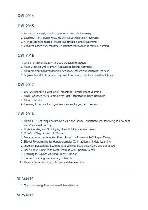
ICML2014ICML20151. An embarrassingly simple approach to zero-shot learning2. Learning Transferable Features with Deep Adaptation Networks3. A Theoretical Analysis of Metric Hypothesis Transfer Learning4. Gradient-based hyperparameter optimization through reversible learningICML20161. One-Shot Generalization in Deep Generative Models2. Meta-Learning with Memory-Augmented Neural Networks3. Meta-gradient boosted decision tree model for weight and target learning4. Asymmetric Multi-task Learning based on Task Relatedness and ConfidenceICML20171. DARLA: Improving Zero-Shot Transfer in Reinforcement Learning2. Model-Agnostic Meta-Learning for Fast Adaptation of Deep Networks3. Meta Networks4. Learning to learn without gradient descent by gradient descentICML20181. MSplit LBI: Realizing Feature Selection and Dense Estimation Simultaneously in Few-shotand Zero-shot Learning2. Understanding and Simplifying One-Shot Architecture Search3. One-Shot Segmentation in Clutter4. Meta-Learning by Adjusting Priors Based on Extended PAC-Bayes Theory5. Bilevel Programming for Hyperparameter Optimization and Meta-Learning6. Gradient-Based Meta-Learning with Learned Layerwise Metric and Subspace7. Been There, Done That: Meta-Learning with Episodic Recall8. Learning to Explore via Meta-Policy Gradient9. Transfer Learning via Learning to Transfer10. Rapid adaptation with conditionally shifted neuronsNIPS20141. Zero-shot recognition with unreliable attributesNIPS2015NIPS20161. Learning feed-forward one-shot learners2. Matching Networks for One Shot Learning3. Learning from Small Sample Sets by Combining Unsupervised Meta-Training with CNNs NIPS20171. One-Shot Imitation Learning2. Few-Shot Learning Through an Information Retrieval Lens3. Prototypical Networks for Few-shot Learning4. Few-Shot Adversarial Domain Adaptation5. A Meta-Learning Perspective on Cold-Start Recommendations for Items6. Neural Program Meta-InductionNIPS20181. Bayesian Model-Agnostic Meta-Learning2. The Importance of Sampling inMeta-Reinforcement Learning3. MetaAnchor: Learning to Detect Objects with Customized Anchors4. MetaGAN: An Adversarial Approach to Few-Shot Learning5. Regret bounds for meta Bayesian optimization with an unknown Gaussian process prior6. Meta-Gradient Reinforcement Learning7. Meta-Reinforcement Learning of Structured Exploration Strategies8. Meta-Learning MCMC Proposals9. Probabilistic Model-Agnostic Meta-Learning10. MetaReg: Towards Domain Generalization using Meta-Regularization11. Zero-Shot Transfer with Deictic Object-Oriented Representation in Reinforcement Learning12. Uncertainty-Aware Few-Shot Learning with Probabilistic Model-Agnostic Meta-Learning13. Multitask Reinforcement Learning for Zero-shot Generalization with Subtask Dependencies14. Stacked Semantics-Guided Attention Model for Fine-Grained Zero-Shot Learning15. Delta-encoder: an effective sample synthesis method for few-shot object recognition16. One-Shot Unsupervised Cross Domain Translation17. Generalized Zero-Shot Learning with Deep Calibration Network18. Domain-Invariant Projection Learning for Zero-Shot Recognition19. Low-shot Learning via Covariance-Preserving Adversarial Augmentation Network20. Improved few-shot learning with task conditioning and metric scaling21. Adapted Deep Embeddings: A Synthesis of Methods for k-Shot Inductive Transfer Learning22. Learning to Play with Intrinsically-Motivated Self-Aware Agents23. Learning to Teach with Dynamic Loss Functiaons24. Memory Replay GANs: learning to generate images from new categories without forgettingICCV20151. One Shot Learning via Compositions of Meaningful Patches2. Unsupervised Domain Adaptation for Zero-Shot Learning3. Active Transfer Learning With Zero-Shot Priors: Reusing Past Datasets for Future Tasks4. Zero-Shot Learning via Semantic Similarity Embedding5. Semi-Supervised Zero-Shot Classification With Label Representation Learning6. Predicting Deep Zero-Shot Convolutional Neural Networks Using Textual Descriptions7. Learning to Transfer: Transferring Latent Task Structures and Its Application to Person-Specific Facial Action Unit DetectionICCV20171. Supplementary Meta-Learning: Towards a Dynamic Model for Deep Neural Networks2. Attributes2Classname: A Discriminative Model for Attribute-Based Unsupervised Zero-ShotLearning3. Low-Shot Visual Recognition by Shrinking and Hallucinating Features4. Predicting Visual Exemplars of Unseen Classes for Zero-Shot Learning5. Learning Discriminative Latent Attributes for Zero-Shot Classification6. Spatial-Aware Object Embeddings for Zero-Shot Localization and Classification of ActionsCVPR20141. COSTA: Co-Occurrence Statistics for Zero-Shot Classification2. Zero-shot Event Detection using Multi-modal Fusion of Weakly Supervised Concepts3. Learning to Learn, from Transfer Learning to Domain Adaptation: A Unifying Perspective CVPR20151. Zero-Shot Object Recognition by Semantic Manifold DistanceCVPR20162. Multi-Cue Zero-Shot Learning With Strong Supervision3. Latent Embeddings for Zero-Shot Classification4. One-Shot Learning of Scene Locations via Feature Trajectory Transfer5. Less Is More: Zero-Shot Learning From Online Textual Documents With Noise Suppression6. Synthesized Classifiers for Zero-Shot Learning7. Recovering the Missing Link: Predicting Class-Attribute Associations for UnsupervisedZero-Shot Learning8. Fast Zero-Shot Image Tagging9. Zero-Shot Learning via Joint Latent Similarity Embedding10. Learning to Read Chest X-Rays: Recurrent Neural Cascade Model for Automated ImageAnnotation11. Learning to Co-Generate Object Proposals With a Deep Structured Network12. Learning to Select Pre-Trained Deep Representations With Bayesian Evidence Framework13. DeepStereo: Learning to Predict New Views From the World’s ImageryCVPR20171. One-Shot Video Object Segmentation2. FastMask: Segment Multi-Scale Object Candidates in One Shot3. Few-Shot Object Recognition From Machine-Labeled Web Images4. From Zero-Shot Learning to Conventional Supervised Classification: Unseen Visual DataSynthesis5. Learning a Deep Embedding Model for Zero-Shot Learning6. Low-Rank Embedded Ensemble Semantic Dictionary for Zero-Shot Learning7. Multi-Attention Network for One Shot Learning8. Zero-Shot Action Recognition With Error-Correcting Output Codes9. One-Shot Metric Learning for Person Re-Identification10. Semantic Autoencoder for Zero-Shot Learning11. Zero-Shot Recognition Using Dual Visual-Semantic Mapping Paths12. Matrix Tri-Factorization With Manifold Regularizations for Zero-Shot Learning13. One-Shot Hyperspectral Imaging Using Faced Reflectors14. Gaze Embeddings for Zero-Shot Image Classification15. Zero-Shot Learning - the Good, the Bad and the Ugly16. Link the Head to the “Beak”: Zero Shot Learning From Noisy Text Description at PartPrecision17. Semantically Consistent Regularization for Zero-Shot Recognition18. Semantically Consistent Regularization for Zero-Shot Recognition19. Zero-Shot Classification With Discriminative Semantic Representation Learning20. Learning to Detect Salient Objects With Image-Level Supervision21. Quad-Networks: Unsupervised Learning to Rank for Interest Point DetectionCVPR20181. A Generative Adversarial Approach for Zero-Shot Learning From Noisy Texts2. Transductive Unbiased Embedding for Zero-Shot Learning3. Zero-Shot Visual Recognition Using Semantics-Preserving Adversarial EmbeddingNetworks4. Learning to Compare: Relation Network for Few-Shot Learning5. One-Shot Action Localization by Learning Sequence Matching Network6. Multi-Label Zero-Shot Learning With Structured Knowledge Graphs7. “Zero-Shot” Super-Resolution Using Deep Internal Learning8. Low-Shot Learning With Large-Scale Diffusion9. CLEAR: Cumulative LEARning for One-Shot One-Class Image Recognition10. Zero-Shot Sketch-Image Hashing11. Structured Set Matching Networks for One-Shot Part Labeling12. Memory Matching Networks for One-Shot Image Recognition13. Generalized Zero-Shot Learning via Synthesized Examples14. Dynamic Few-Shot Visual Learning Without Forgetting15. Exploit the Unknown Gradually: One-Shot Video-Based Person Re-Identification byStepwise Learning16. Feature Generating Networks for Zero-Shot Learning17. Low-Shot Learning With Imprinted Weights18. Zero-Shot Recognition via Semantic Embeddings and Knowledge Graphs19. Webly Supervised Learning Meets Zero-Shot Learning: A Hybrid Approach for Fine-Grained Classification20. Few-Shot Image Recognition by Predicting Parameters From Activations21. Low-Shot Learning From Imaginary Data22. Discriminative Learning of Latent Features for Zero-Shot Recognition23. Multi-Content GAN for Few-Shot Font Style Transfer24. Preserving Semantic Relations for Zero-Shot Learning25. Zero-Shot Kernel Learning26. Neural Style Transfer via Meta Networks27. Learning to Estimate 3D Human Pose and Shape From a Single Color Image28. Learning to Segment Every Thing29. Leveraging Unlabeled Data for Crowd Counting by Learning to Rank。

深度学习论⽂汇总本博客⽤于记录⾃⼰平时收集的⼀些不错的深度学习论⽂，近9成的⽂章都是引⽤量3位数以上的论⽂，剩下少部分来⾃个⼈喜好，本博客将伴随着我的研究⽣涯长期更新，如有错误或者推荐⽂章烦请私信。

深度学习书籍和⼊门资源LeCun Y, Bengio Y, Hinton G. Deep learning[J]. Nature, 2015, 521(7553): 436-444.（深度学习最权威的综述）Bengio, Yoshua, Ian J. Goodfellow, and Aaron Courville. Deep learning. An MIT Press book. (2015).（深度学习经典书籍）Deep Learning Tutorial（李宏毅的深度学习综述PPT，适合⼊门）D L. LISA Lab[J]. University of Montreal, 2014.（Theano配套的深度学习教程）deeplearningbook-chinese （深度学习中⽂书，⼤家⼀起翻译的）早期的深度学习Hecht-Nielsen R. Theory of the backpropagation neural network[J]. Neural Networks, 1988, 1(Supplement-1): 445-448.（BP神经⽹络）Hinton G E, Osindero S, Teh Y W. A fast learning algorithm for deep belief nets.[J]. Neural Computation, 2006, 18(7):1527-1554.（深度学习的开端DBN）Hinton G E, Salakhutdinov R R. Reducing the dimensionality of data with neural networks.[J]. Science, 2006, 313(5786):504-7.（⾃编码器降维）Ng A. Sparse autoencoder[J]. CS294A Lecture notes, 2011, 72(2011): 1-19.（稀疏⾃编码器）Vincent P, Larochelle H, Lajoie I, et al. Stacked denoising autoencoders: Learning useful representations in a deep network with a local denoising criterion[J]. Journal of Machine Learning Research, 2010, 11(Dec): 3371-3408.（堆叠⾃编码器，SAE）深度学习的爆发:ImageNet挑战赛Krizhevsky, Alex, Ilya Sutskever, and Geoffrey E. Hinton. Imagenet classification with deep convolutional neural networks. Advances in neural information processing systems. 2012.（AlexNet）Simonyan, Karen, and Andrew Zisserman. Very deep convolutional networks for large-scale image recognition. arXiv preprint arXiv:1409.1556 (2014).（VGGNet）Szegedy, Christian, et al. Going deeper with convolutions. Proceedings of the IEEE Conference on Computer Vision and Pattern Recognition. 2015. （GoogLeNet）Szegedy C, Vanhoucke V, Ioffe S, et al. Rethinking the Inception Architecture for Computer Vision[J]. Computer Science, 2015:2818-2826.（InceptionV3）He, Kaiming, et al. Deep residual learning for image recognition. arXiv preprint arXiv:1512.03385 (2015).（ResNet）Chollet F. Xception: Deep Learning with Depthwise Separable Convolutions[J]. arXiv preprint arXiv:1610.02357, 2016.（Xception）Huang G, Liu Z, Weinberger K Q, et al. Densely Connected Convolutional Networks[J]. 2016. (DenseNet, 2017 CVPR best paper) Squeeze-and-Excitation Networks. (SeNet, 2017 ImageNet 冠军)Zhang X, Zhou X, Lin M, et al. Shufflenet: An extremely efficient convolutional neural network for mobile devices[J]. arXiv preprint arXiv:1707.01083, 2017.（Shufflenet）Sabour S, Frosst N, Hinton G E. Dynamic routing between capsules[C]//Advances in Neural Information Processing Systems. 2017: 3859-3869.（Hinton, capsules）炼丹技巧Srivastava N, Hinton G E, Krizhevsky A, et al. Dropout: a simple way to prevent neural networks from overfitting[J]. Journal of Machine Learning Research, 2014, 15(1): 1929-1958.（Dropout）Ioffe S, Szegedy C. Batch normalization: Accelerating deep network training by reducing internal covariate shift[J]. arXiv preprint arXiv:1502.03167, 2015.（Batch Normalization）Lin M, Chen Q, Yan S. Network In Network[J]. Computer Science, 2014.（Global average pooling的灵感来源）Goyal, Priya, Dollár, Piotr, Girshick, Ross, et al. Accurate, Large Minibatch SGD: Training ImageNet in 1 Hour[J]. 2017. （Facebook实验室的成果，解决了⼯程上⽹络batchsize特⼤时性能下降的问题）递归神经⽹络Mikolov T, Karafiát M, Burget L, et al. Recurrent neural network based language model[C]//Interspeech. 2010, 2: 3.（RNN和语language model结合较经典⽂章）Kamijo K, Tanigawa T. Stock price pattern recognition-a recurrent neural network approach[C]//Neural Networks, 1990., 1990 IJCNN International Joint Conference on. IEEE, 1990: 215-221.（RNN预测股价）Hochreiter S, Schmidhuber J. Long short-term memory[J]. Neural computation, 1997, 9(8): 1735-1780.（LSTM的数学原理）Sak H, Senior A W, Beaufays F. Long short-term memory recurrent neural network architectures for large scale acousticmodeling[C]//Interspeech. 2014: 338-342.（LSTM进⾏语⾳识别）Chung J, Gulcehre C, Cho K H, et al. Empirical evaluation of gated recurrent neural networks on sequence modeling[J]. arXiv preprint arXiv:1412.3555, 2014.（GRU⽹络）Ling W, Luís T, Marujo L, et al. Finding function in form: Compositional character models for open vocabulary word representation[J].arXiv preprint arXiv:1508.02096, 2015.（LSTM在词向量中的应⽤）Huang Z, Xu W, Yu K. Bidirectional LSTM-CRF models for sequence tagging[J]. arXiv preprint arXiv:1508.01991, 2015.（Bi-LSTM在序列标注中的应⽤）注意⼒模型Bahdanau D, Cho K, Bengio Y. Neural machine translation by jointly learning to align and translate[J]. arXiv preprintarXiv:1409.0473, 2014.（Attention model的提出）Mnih V, Heess N, Graves A. Recurrent models of visual attention[C]//Advances in neural information processing systems. 2014: 2204-2212.（Attention model和视觉结合）Xu K, Ba J, Kiros R, et al. Show, Attend and Tell: Neural Image Caption Generation with Visual Attention[C]//ICML. 2015, 14: 77-81.（Attention model⽤于image caption的经典⽂章）Lee C Y, Osindero S. Recursive Recurrent Nets with Attention Modeling for OCR in the Wild[C]//Proceedings of the IEEE Conference on Computer Vision and Pattern Recognition. 2016: 2231-2239.（Attention model ⽤于OCR）Gregor K, Danihelka I, Graves A, et al. DRAW: A recurrent neural network for image generation[J]. arXiv preprint arXiv:1502.04623, 2015.（DRAM，结合Attention model的图像⽣成）⽣成对抗⽹络Goodfellow I, Pouget-Abadie J, Mirza M, et al. Generative adversarial nets[C]//Advances in neural information processing systems.2014: 2672-2680.（GAN的提出，挖坑⿐祖）Mirza M, Osindero S. Conditional generative adversarial nets[J]. arXiv preprint arXiv:1411.1784, 2014.（CGAN）Radford A, Metz L, Chintala S. Unsupervised representation learning with deep convolutional generative adversarial networks[J].arXiv preprint arXiv:1511.06434, 2015.（DCGAN）Denton E L, Chintala S, Fergus R. Deep Generative Image Models using a Laplacian Pyramid of Adversarial Networks[C]//Advances in neural information processing systems. 2015: 1486-1494.（LAPGAN）Chen X, Duan Y, Houthooft R, et al. Infogan: Interpretable representation learning by information maximizing generative adversarial nets[C]//Advances in Neural Information Processing Systems. 2016: 2172-2180.（InfoGAN）Arjovsky M, Chintala S, Bottou L. Wasserstein gan[J]. arXiv preprint arXiv:1701.07875, 2017.（WGAN）Zhu J Y, Park T, Isola P, et al. Unpaired image-to-image translation using cycle-consistent adversarial networks[J]. arXiv preprint arXiv:1703.10593, 2017.（CycleGAN）Yi Z, Zhang H, Gong P T. DualGAN: Unsupervised Dual Learning for Image-to-Image Translation[J]. arXiv preprint arXiv:1704.02510, 2017.（DualGAN）Isola P, Zhu J Y, Zhou T, et al. Image-to-image translation with conditional adversarial networks[J]. arXiv preprint arXiv:1611.07004, 2016.（pix2pix）⽬标检测Szegedy C, Toshev A, Erhan D. Deep neural networks for object detection[C]//Advances in Neural Information Processing Systems.2013: 2553-2561.（深度学习早期的物体检测）Girshick, Ross, et al. Rich feature hierarchies for accurate object detection and semantic segmentation. Proceedings of the IEEE conference on computer vision and pattern recognition. 2014.（RCNN）He K, Zhang X, Ren S, et al. Spatial pyramid pooling in deep convolutional networks for visual recognition[C]//European Conference on Computer Vision. Springer International Publishing, 2014: 346-361.（何凯明⼤神的SPPNet）Girshick R. Fast r-cnn[C]//Proceedings of the IEEE International Conference on Computer Vision. 2015: 1440-1448.（速度更快的Fast R-cnn）Ren S, He K, Girshick R, et al. Faster r-cnn: Towards real-time object detection with region proposal networks[C]//Advances in neural information processing systems. 2015: 91-99.（速度更更快的Faster r-cnn）Redmon J, Divvala S, Girshick R, et al. You only look once: Unified, real-time object detection[C]//Proceedings of the IEEEConference on Computer Vision and Pattern Recognition. 2016: 779-788.（实时⽬标检测YOLO）Liu W, Anguelov D, Erhan D, et al. SSD: Single shot multibox detector[C]//European Conference on Computer Vision. Springer International Publishing, 2016: 21-37.（SSD）Li Y, He K, Sun J. R-fcn: Object detection via region-based fully convolutional networks[C]//Advances in Neural InformationProcessing Systems. 2016: 379-387.（R-fcn）Lin T Y, Goyal P, Girshick R, et al. Focal loss for dense object detection[J]. arXiv preprint arXiv:1708.02002, 2017.（Focal loss）One/Zero shot learningFei-Fei L, Fergus R, Perona P. One-shot learning of object categories[J]. IEEE transactions on pattern analysis and machineintelligence, 2006, 28(4): 594-611.（One shot learning）Larochelle H, Erhan D, Bengio Y. Zero-data learning of new tasks[J]. 2008:646-651.（Zero shot learning的提出）Palatucci M, Pomerleau D, Hinton G E, et al. Zero-shot learning with semantic output codes[C]//Advances in neural information processing systems. 2009: 1410-1418.（Zero shot learning⽐较经典的应⽤）图像分割Long J, Shelhamer E, Darrell T. Fully convolutional networks for semantic segmentation[C]//Proceedings of the IEEE Conference on Computer Vision and Pattern Recognition. 2015: 3431-3440.（有点⽼但是⾮常经典的图像语义分割论⽂，CVPR2015）Chen L C, Papandreou G, Kokkinos I, et al. Deeplab: Semantic image segmentation with deep convolutional nets, atrous convolution, and fully connected crfs[J]. arXiv preprint arXiv:1606.00915, 2016.（DeepLab）Zhao H, Shi J, Qi X, et al. Pyramid scene parsing network[J]. arXiv preprint arXiv:1612.01105, 2016.（PSPNet）Yu F, Koltun V, Funkhouser T. Dilated residual networks[J]. arXiv preprint arXiv:1705.09914, 2017.He K, Gkioxari G, Dollár P, et al. Mask R-CNN[J]. arXiv preprint arXiv:1703.06870, 2017.（何凯明⼤神的MASK r-cnn，膜）Hu R, Dollár P, He K, et al. Learning to Segment Every Thing[J]. arXiv preprint arXiv:1711.10370, 2017.（Mask Rcnn增强版）-Person Re-IDYi D, Lei Z, Liao S, et al. Deep metric learning for person re-identification[C]//Pattern Recognition (ICPR), 2014 22nd International Conference on. IEEE, 2014: 34-39.（较早的⼀篇基于CNN的度量学习的Re-ID，现在来看⽹络已经很简单了）Ding S, Lin L, Wang G, et al. Deep feature learning with relative distance comparison for person re-identification[J]. PatternRecognition, 2015, 48(10): 2993-3003.（triplet loss）Cheng D, Gong Y, Zhou S, et al. Person re-identification by multi-channel parts-based cnn with improved triplet lossfunction[C]//Proceedings of the IEEE Conference on Computer Vision and Pattern Recognition. 2016: 1335-1344.（improved triplet loss）Hermans A, Beyer L, Leibe B. In Defense of the Triplet Loss for Person Re-Identification[J]. arXiv preprint arXiv:1703.07737, 2017.（Triplet loss with hard mining sample）Chen W, Chen X, Zhang J, et al. Beyond triplet loss: a deep quadruplet network for person re-identification[J]. arXiv preprintarXiv:1704.01719, 2017.（四元组）Zheng Z, Zheng L, Yang Y. Unlabeled samples generated by gan improve the person re-identification baseline in vitro[J]. arXiv preprint arXiv:1701.07717, 2017.(⽤GAN造图做ReID第⼀篇)Zhang X, Luo H, Fan X, et al. AlignedReID: Surpassing Human-Level Performance in Person Re-Identification[J]. arXiv preprint arXiv:1711.08184, 2017. （AlignedReid，⾸次超越⼈类）（在这个领域提供了⼤量论⽂，常⽤的数据集和代码都可以在主页中找到）本⽂转载，原⽂链接：/qq_21190081/article/details/69564634。