Realistic propagation simulation of urban mesh networks

波动方程第三类边界条件The wave equation, a fundamental concept in physics, governs the behavior of waves in various mediums. It is a partial differential equation that describes how the amplitude of the wave varies with time and space. When studying wave propagation, it is crucial to consider the boundary conditions, which specify the behavior of the wave at the edges of the system. The third type of boundary condition, also known as the mixed boundary condition, combines features of both Dirichlet and Neumann boundary conditions.波动方程是物理学中的一个基本概念，它支配着各种介质中波的行为。

作为一个偏微分方程，它描述了波的振幅如何随时间和空间变化。

在研究波动传播时，考虑边界条件至关重要，因为边界条件规定了波在系统边缘的行为。

第三类边界条件，也称为混合边界条件，结合了Dirichlet边界条件和Neumann边界条件的特征。

In the context of the wave equation, the third type of boundary condition specifies that a combination of the value of the wave function and its derivative at a given boundary must satisfy certain conditions. This allows for more flexibility in modeling real-world systems, where waves may interact with complex boundaries in various ways. For instance, in acoustics, the reflection and transmission of sound waves at a wall or an obstacle can be modeled using this type of boundary condition.在波动方程的上下文中，第三类边界条件规定了在给定边界上，波函数的值及其导数必须满足某些条件。

虚实融合英语Integration of the Real and the Virtual WorldIntroduction:In today's rapidly advancing world, the integration of the real and the virtual has become a prominent and relevant topic of discussion. With the advancements in technology, the line between what is real and what is virtual has blurred significantly. This article aims to explore the concept of virtual reality and its impact on our lives, education, and entertainment.1. The Definition of Virtual Reality:Virtual reality (VR) refers to a computer-generated simulation of an environment that can be interacted with by a person through sensory devices, such as a headset or gloves. It provides a realistic experience that can simulate various scenarios, whether they are based on real-world locations or imaginative settings.2. Applications in Education:2.1 Virtual Field Trips:One of the significant advantages of VR in education is its ability to provide virtual field trips. With VR technology, students can virtually visit historical landmarks, explore space, or dive into the depths of the ocean. This immersive experience enhances learning by allowing students to see and experience things beyond the limitations of the traditional classroom.2.2 Simulations and Training:VR also enables hands-on training and simulations, particularly in complex fields like medicine and engineering. Students can practice surgical procedures or engineering designs in a virtual environment, providing a safe and controlled space for learning before transitioning to real-world scenarios.3. Impacts on Entertainment and Gaming:3.1 Immersive Gaming Experience:VR has revolutionized the gaming industry by offering an immersive experience. With a VR headset, players can dive into virtual worlds, interact with objects, and engage in realistic gameplay. This technology has taken entertainment to a new level, giving gamers a more engaging and interactive experience.3.2 Virtual Reality Movies and Experiences:In addition to gaming, VR has brought a new dimension to the world of movies and entertainment. Virtual reality movies and experiences allow viewers to be fully immersed in a story, making them active participants rather than passive viewers. It provides a sense of presence and empowers the audience to explore and interact with the narrative in unique ways.4. Challenges and Limitations:4.1 Cost and Accessibility:One of the major challenges of VR technology is its cost. High-quality VR headsets and equipment can be expensive, limiting widespread adoption, particularly in developing countries. Additionally, not everyone has accessto the necessary hardware and devices required for a seamless VR experience.4.2 Health and Safety Considerations:Extended exposure to VR can lead to symptoms known as VR sickness, including nausea, dizziness, and eye strain. To ensure the well-being of users, developers and designers need to consider the potential side effects and work towards minimizing the risks associated with prolonged VR usage.Conclusion:The integration of the real and the virtual world through virtual reality offers significant opportunities in various fields, including education and entertainment. From virtual field trips in education to immersive gaming experiences, VR has the potential to transform how we learn, play, and interact with the digital realm. However, the challenges of cost and accessibility, as well as health and safety concerns, need to be addressed to ensure that this technology can be widely utilized and enjoyed by people from all walks of life. With continued advancements, virtual reality has the potential to shape our future in ways we can only imagine.。

I. IntroductionIn the realm of engineering, delivering projects that meet or exceed high-quality and high-standard benchmarks is not merely a desirable objective but an imperative for ensuring long-term functionality, safety, cost-effectiveness, and environmental sustainability. This comprehensive engineering plan outlines a multifaceted approach that integrates various strategies, processes, and tools to achieve these stringent targets across diverse project dimensions. The plan, spanning over 1267 words, delves into key aspects such as project planning, design excellence, materials and construction methodologies, quality control, stakeholder engagement, risk management, and continuous improvement, offering a holistic perspective on how to engineer excellence.II. Project Planning: Setting the Foundation for Quality and StandardsA. Clear Objectives and Scope DefinitionThe foundation of any high-quality, high-standard engineering project lies in establishing clear, concise, and measurable objectives aligned with stakeholders' expectations and regulatory requirements. These objectives should encompass technical performance, cost, schedule, environmental impact, and social considerations. A well-defined scope statement, outlining the boundaries of the project, serves as a reference point for decision-making and prevents scope creep, which can compromise quality and standards.B. Robust Work Breakdown Structure (WBS) and ScheduleDeveloping a detailed WBS ensures that all project tasks are identified, organized, and assigned appropriately, fostering accountability and facilitating effective monitoring. Integrating this WBS into a realistic, resource-loaded project schedule, incorporating milestones, dependencies, and contingencies, enables proactive management of time constraints, a critical factor in maintaining quality and adhering to standards.C. Budget Estimation and Cost ControlAccurate budget estimation, utilizing parametric or historical data, expert judgment, and appropriate contingency provisions, is vital for securing sufficient funding and preventing cost overruns that could force trade-offs between quality and standards. Implementing rigorous cost control mechanisms, including regular budget reviews, change order management, and value engineering exercises, helps maintain financial discipline throughout the project lifecycle.III. Design Excellence: Innovating for Optimal Performance and ComplianceA. Performance-Based DesignAdopting a performance-based design approach focuses on achieving specific functional, environmental, and aesthetic outcomes rather than merely adhering to prescriptive codes and standards. This method encourages innovation, optimizes resource utilization, and ensures that the final product meets or exceeds intended performance criteria.B. Sustainable Design PrinciplesIntegrating sustainable design principles, such as energy efficiency, material selection, water conservation, and waste reduction, not only enhances the project's environmental footprint but can also contribute to improved quality and longer service life. Utilizing green building rating systems, such as LEED or BREEAM, provides a structured framework for assessing and enhancing the project's sustainability credentials.C. Advanced Modeling and SimulationEmploying advanced computational tools like Building Information Modeling (BIM), Finite Element Analysis (FEA), and Computational Fluid Dynamics (CFD) allows for precise prediction of structural behavior, energy performance, and other critical parameters. This facilitates informed decision-making, reduces errors, and enhances overall design quality and compliance with standards.IV. Materials and Construction Methodologies: Ensuring Durability and EfficiencyA. Material Selection and SpecificationChoosing materials with proven durability, low maintenance requirements, and minimal environmental impact is crucial for achieving high-quality, high-standard outcomes. Adhering to relevant material standards, conducting thorough supplier evaluations, and implementing strict inspection and testing protocols help ensure material quality and consistency.B. Innovative Construction Techniques and TechnologiesEmbracing innovative construction techniques, such as prefabrication, modularization, and digital construction, can enhance productivity, reduce onsite errors, and improve overall build quality. Additionally, leveraging emerging technologies like drones, robotics, and augmented reality can further enhance construction accuracy, safety, and efficiency.V. Quality Control: Systematic Monitoring and VerificationA. Comprehensive Quality Management SystemImplementing a robust quality management system (QMS), based on international standards like ISO 9001, provides a structured framework for planning, executing, and monitoring all quality-related activities throughout the project lifecycle. Key components of a QMS include quality policies, procedures, work instructions, and documentation controls.B. In-process Inspections and TestingConducting regular in-process inspections and non-destructive testing at critical stages of the project helps identify and rectify defects early, preventing their propagation and minimizing rework. Employing advanced inspection technologies, such as thermal imaging, ultrasonic testing, and 3D laser scanning, enhances detection accuracy and efficiency.C. Independent Third-party VerificationEngaging independent third-party verification agencies to assess compliance with design specifications, codes, and standards adds an extra layer of assurance to the quality control process. Their unbiased assessments can help identify potential issues, provide valuable feedback for improvement, andbolster stakeholders' confidence in the project's quality and standard adherence.VI. Stakeholder Engagement: Collaborative Governance for Enhanced OutcomesA. Proactive Communication and ConsultationEstablishing open channels of communication with stakeholders, including clients, end-users, regulatory bodies, and the broader community, fosters transparency, understanding, and trust. Regular project updates, public consultations, and user-group workshops enable stakeholders to provide feedback, voice concerns, and contribute to decision-making, ultimately enhancing project quality and alignment with standards.B. Partnering and AlliancingFormal partnering and alliancing arrangements among project participants, such as designers, contractors, and suppliers, promote a collaborative, non-adversarial environment conducive to sharing knowledge, resources, and risks. This collective commitment to project success often results in enhanced problem-solving, innovation, and overall quality and standard attainment.VII. Risk Management: Anticipating and Mitigating Threats to Quality and StandardsA. Comprehensive Risk AssessmentConducting a thorough risk assessment at the outset of the project, involving cross-functional teams and stakeholders, helps identify potential threats to quality and standard compliance. Risks should be analyzed in terms of likelihood, impact, and velocity, enabling prioritization and allocation of resources for mitigation efforts.B. Risk Response StrategiesDeveloping tailored risk response strategies for each identified risk, including avoidance, transfer, mitigation, or acceptance, ensures that risks are effectively managed throughout the project lifecycle. Regular risk review meetings and real-time risk monitoring using dedicated software platforms help maintain risk visibility and responsiveness.C. Contingency PlanningEstablishing contingency plans for high-priority risks, outlining actions to be taken in the event of risk realization, ensures swift and coordinated responses that minimize impacts on project quality and standard adherence. Adequate provisioning of contingency funds and resources further bolsters the project's resilience against unforeseen events.VIII. Continuous Improvement: Learning from Experience to Enhance Future OutcomesA. Post-Project Reviews and Lessons LearnedConducting post-project reviews, facilitated by an independent facilitator, encourages open discussion and identification of successes, challenges, and areas for improvement. Documenting and disseminating lessons learned within the organization and the broader industry contributes toorganizational learning and the continuous enhancement of quality and standard practices.B. Benchmarking and Best Practice AdoptionRegularly benchmarking project performance against industry standards, peers, and best practices helps identify gaps and opportunities for improvement. Actively seeking out and adopting proven best practices from within and outside the industry accelerates the organization's learning curve and enhances its ability to deliver high-quality, high-standard projects consistently.ConclusionAchieving high-quality, high-standard outcomes in engineering projects necessitates a holistic, multidimensional approach that encompasses meticulous planning, design excellence, judicious material and construction choices, rigorous quality control, inclusive stakeholder engagement, proactive risk management, and a commitment to continuous improvement. By diligently implementing the strategies outlined in this comprehensive engineering plan, organizations can enhance their capacity to deliver projects that not only meet but surpass stakeholders' expectations and contribute to the advancement of the engineering profession.。

For office use onlyT1________________ T2________________ T3________________ T4________________Team Control Number22599Problem ChosenAFor office use onlyF1________________F2________________F3________________F4________________ 2013Mathematical Contest in Modeling(MCM/ICM)Summary Sheet(Attach a copy of this page to your solution paper.)Heat Radiation in The OvenHeat distribution of pans in the oven is quite different from each other,which depends on their shapes.Thus,our model aims at two goals.One is to analyze the heat distri-bution in different ovens based on the locations of electrical heating cubes.Further-more,a series of heat distribution which varies from circular pans to rectangular pans could be got easily.The other is to optimize the pans placing,in order to choose a best way to maximize the even heat and the number of pans at the same time.Mathematically speaking,our solution consists of two models,analyzing and optimi-zing.In part one,our whole-local approach shows the heat distribution of every pan.Firstly,we use the Stefan-Boltzmann law and Fourier theorem to describe the heat distribution in the air around the electrical heating tube.And then, based on plane in-tercept method and simplified Monte Carlo method,the heat distribution of different shapes of pans is obtained.Finally,we explain the phenomenon that the corners of a pan always get over heated with water waves stirring by analogy.In part two,our discretize-convert approach optimizes the shape and number of the pans.Above all,we discre-tize the side length of the oven, so that the number and the average heat of the pans vary linearly.In the end,the abstract weight P is converted into a specific length,in order to reach a compromise between the two factors.Specially,we create a unique method to convert the variables from the whole space to the local section.The special method allows us to draw the heat distribution of every single section in the oven.The algorithm we create does a great job in flexibility,which can be applied to all shapes of pans.Type a summary of your results on this page.Do not includethe name of your school,advisor,or team members on this page.Heat Radiation in The OvenSummaryHeat distribution of pans in the oven is quite different from each other,which depends on their shapes.Thus,our model aims at two goals.One is to analyze the heat distri-bution in different ovens based on the locations of electrical heating cubes.Further-more,a series of heat distribution which varies from circular pans to rectangular pans could be got easily.The other is to optimize the pans placing,in order to choose a best way to maximize the even heat and the number of pans at the same time.Mathematically speaking,our solution consists of two models,analyzing and optimi-zing.In part one,our whole-local approach shows the heat distribution of every pan. Firstly,we use the Stefan-Boltzmann law and Fourier theorem to describe the heat distribution in the air around the electrical heating tube.And then,based on plane in-tercept method and simplified Monte Carlo method,the heat distribution of different shapes of pans is obtained.Finally,we explain the phenomenon that the corners of a pan always get over heated with water waves stirring by analogy.In part two,our discretize-convert approach optimizes the shape and number of the pans.Above all, we discre-tize the side length of the oven,so that the number and the average heat of the pans vary linearly.In the end,the abstract weight P is converted into a specific length,in order to reach a compromise between the two factors.Specially,we create a unique method to convert the variables from the whole space to the local section.The special method allows us to draw the heat distribution of every single section in the oven.The algorithm we create does a great job in flexibility, which can be applied to all shapes of pans.Keywords:Monte Carlo thermal radiation section heat distribution discretizationIntroductionMany studies on heat conduction wasted plenty of time in solving the partial differential equations,since it’s difficult to solve even for computers.We turn to another way to work it out.Firstly,we study the heat radiation instead of heat conduction to keep away from the sophisticated partial differential equations.Then, we create a unique method to convert every variable from the whole space to section. In other words,we work everything out in heat radiation and convert them into heat contradiction.AssumptionsWe make the following assumptions about the distribution of heat in this paper.·Initially two racks in the oven,evenly spaced.·When heating the electrical heating tubes,the temperature of which changes from room temperature to the desired temperature.It takes such a short time that we can ignore it.·Different pans are made in same material,so they have the same rate of heat conduction.·The inner walls of the oven are blackbodies.The pan is a gray body.The inner walls of the oven absorb heat only and reflect no heat.·The heat can only be reflected once when rebounded from the pan.Heat Distribution ModelOur approach involves four steps:·Use the Fourier theorem to calculate the loss energy when energy beams are spread in the medium.So we can get the heat distribution around each electrical heating tube.The heat distribution of the entire space could be go where the heat of two electrical heating tubes cross together.·When different shapes of the pans are inserted into the oven,the heat map of the entire space is crossed by the section of the pan.Thus,the heat map of every single pan is obtained.·Establish a suitable model to get the reflectivity of every single point on the pan with the simplified Monte Carlo method.And then,a final heat distribution map of the pan without reflection loss is obtained.·A realistic conclusion is drawn due to the results of our model compared with water wave propagation phenomena.First of all,the paper will give a description of the initial energy of the electrical hea-ting tube.We see it as a blackbody who reflects no heat at all.Electromagnetic know-ledge shows that wavelength of the heat rays ranges from um 110−to um 210as shown below[1]:Figure 1.Figure 2.We apply the Stefan-Boltzmann’s law[2]whose solution is ()1/512−=−T c b e c E λλλ(1)()λλλλλd e c d E E T c b b ∫∫∞−∞−==0/51012(2)Where b E means the ability of blackbody to radiate. 1c and 2c are constants.Obviously,,the initial energy of a black body is )(0122398.320m w e E b ×+=.Combine Figure 1with Figure 2,we integrate (1)from 1λto 2λto get the equation as follow:λλλλλλd E E b b ∫=−2121)((3)Figure 3.From Figure 3,it can be seen how the power of radiation varies with wavelength.Secondly,based on the Fourier theorem,the relation between heat and the distance from the electrical heating tubes is:dxdt S Q λ−=(4)Where Q is the power of heat (W s J =/),S is the area where the energy beamradiates (2m ),dxdt represents the temperature gradient along the direction of energy beam.[3]It is known that the energy becomes weaker as the distance becomes larger.According to the fact we know:dxdQ =ρ(5)Where ρis the rate of energy changing.We assume that the desired temperature of electrical heating tube is 500k.With the two equations,the distribution of heat is shown as follow:Figure 4.(a)Figure 4.(b)In order to draw the map of heat distribution in the oven,we use MATLAB to work on the complicated algorithm.The relation between the power of heat and the distance is shown in Figure4(a).The relation between temperature and distance is presented in Figure4(b).The spreading direction of energy beam is presented in Figure5.Figure5.The shape of electrical heating tube is irregular.The heat distribution of a single electrical heating tube can be draw in3D space with MATLAB.The picture is shown in Figure6.After superimposing,the total heat distribution of two tubes is shown below in Figure7and Figure8.Figure6.Figure7.Figure8.The pictures above show the energy in an oven with no pan.We put in a rectangular pan whose area is A,and intercept the maps with MATLAB.The result is show in Figure9.Figure9.Figure10.Put in a circular pan to intercept the maps,whose area is A,also.The distribution of heat is shown in Figure11.Figure11.When put in a pan in transition shape,which is neither rectangular nor circular.The area of it is A,also.The heat distribution on such a pan is shown as follow:Figure12(a)Figure12(b).Figure13.Next,learning from the Monte Carlo simulation[4],a model is established to get obtain the reflectivity.We generate a random number between0and1to determine if the energy beam on certain point is reflected.•Firstly,to demonstrate the question better,we construct a simple model:Figure 14.Where θis the viewing angle from electrical heating tube to the pan.360θ=R is the proportion of the beams radiated to the pan.•What is more,we assume the total beam is 1M .Ideally,the number of absorption is3601θ×M .Then,each element of the pan is seen as a grid point.Each grid point can generate a-3601θ×M -random-number vector between 0and 1in MATLAB.•After MATLAB simulating,the number of beams decreased by 2M ,due to thereflection.So we define a probability θρ12360M M ×=to describe the number of beams reflected.The conclusion is :•If R ≤ρ,the energy beam is absorbed.•If R >ρ,the energy beam is reflected.[5]Based on the analysis above,our model get a final result of heat-distribution on the pan as shown below:Figure 15(a)Figure15(b).The conclusion is known that the closer the shape of pans is to circle,the more evenly the heat is distributed.Moreover,the phenomenon that the corners always get over heated can be explained by water wave propagation in different containers.When there is a fluctuation in the center of the water,the ripples will fluctuate and spread in concentric circles,as shown in Figure16.The fluctuation stirs waves up when contacting the pared with the waves with one boundary,the waves in corner make a higher amplitude.The thermal conduction on the pan is exactly the inverse process of the waves propagation.The range of thermal motion is much smaller than it on the side.That’s why the corners is easy to get over heated.In order to make the heat evenly distributed on the pan,the sides of the pan should be as few as possible.Therefore,if nothing is considered about the utilization of space,a circle pan is the best choice.Figure16,the water waves propagation[6]According to the analysis above and Figure7,the phenomenon shows that the heat conduction is similar to water waves propagation.So it is proved that heatconcentrates in the four corners of the rectangular pan.The Super Pan ModelAssumptions•The width of the oven(W)is mm100,the length is L.•There are three pans at most in vertical direction.•Each pan’s area is A.The first part.Calculate the maximum number of pans in the oven.Different shapes of pan have different heat distribution which affects the number of pans,judging from the previous solution.According to the conclusion in the first model,the heat is distributed the most evenly on a circular pan rather than a rectangular one.However, the rectangular pans make fuller use of the space the space than circular ones.Both factors considered,a polygonal pan is chosen.A circle can be regard as a polygon whose number of boundaries tends to infinity. Except for rectangle,only regular hexagon and equilateral triangle can be closely placed.Because of the edges of equilateral triangle,heat dissipation is worse than rectangle.So,hexagonal pans are adopted after all the discussion.Considering the gaps near boundaries,we place the hexagonal pans closely attached each other on the long side L.There are two kinds of programs as shown below.Program1.Program2.Obviously,Program2is better than Program1when considering space utilization.So scheme 1is adopted.Then,design a size of each hexagonal pan to make the highest space utilization.With the aim of utilization,hexagonal pans has to be placed contact closely with each other on both sides.It is necessary to assume a aspect ratio of the oven to work out the number of pans(N ).Assume that the side length of a regular hexagon is a ,the length-width ratio of the oven is λand L ∆is the increment in discretization.Because the number of pans can not change continuously when ⋅⋅⋅=+∈3,2,1),1,(m m m n ,the equations would be as follows.⎪⎪⎪⎪⎪⎪⎪⎪⎪⎪⎪⎩⎪⎪⎪⎪⎪⎪⎪⎪⎪⎪⎪⎨⎧⎥⎥⎥⎥⎦⎤⎢⎢⎢⎢⎣⎡⋅−====∆⋅+<⎥⎦⎤⎢⎣⎡∆⋅+−∆⋅+≤⋅=∆∆⋅+=<<=a W L n W L N Lk L W W L k L W L k L a L L k L L L W aW 23,810;23105000λ(6)Result:⎪⎪⎩⎪⎪⎨⎧⋅⋅⋅==⋅+=⋅⋅⋅=−=+−⋅+=3,2,1,2233,2,1,1212130201k k n n N N k k n n N N Where 1N represents the number of pans when n is odd,2N represents the number of pans when n is even.The specific number of pans is depended on the width-length ratio of oven.The second part.Maximum the heat distribution of the pans.We define the average heat(H )as the ratio of total heat and total area of the pans.Aiming to get the most average heat,we set the width-length ratio of the oven λ.Space utilization is not considered here.A conclusion is easy to draw from Figure 8that a square area in the oven from 150mm to 350mm in length shares the most heat evenly.So the pans should beplaced mainly in this area.From model1we know that the corners of the oven are apt to gather heat.Besides,four more pans are added in the corners to absorb more heat. Because heat absorbing is the only aim,there is no need to consider space utilization. Circular pans can distribute heat more evenly than any other shape due to model1.So circular pans are used in Figure17.Figure8.Figure17.We set the heat of the pans in the most heated area(the middle row)as Q.Pans in the corners receive more heat but uneven theoretically.And the square of the four pans in the corners is so small compared with the total square that we set the heat of the four as Q too.When the length of oven(L)increases,the number of pans increases too. It makes the square of the gaps between pans bigger,meanwhile.If each pan has a same radius(r)and square(A),the equation about average heat,length-width ratio and number of pans would be(7).⎪⎪⎪⎪⎪⎪⎪⎪⎪⎪⎪⎩⎪⎪⎪⎪⎪⎪⎪⎪⎪⎪⎪⎨⎧=+=⎥⎦⎤⎢⎣⎡⋅−====∆⋅+<⎦⎤⎢⎣⎡∆⋅+−∆⋅+≤⋅=∆∆⋅+=<<⋅=⋅⋅=...3,2,12;71021053410002k nN N r W L n W L N L k L W W L k L W L k L r L L k L L L W r A W r λπ(7)Here we get the most average heat (H ):29400WQ H ⋅=πThe third part.We discussed two different plans in the previous parts of the paper.One is aimed to get the most average heat,while the other aimed to place the most pans.The two plans are contradictory with each other,and can not be achieved together.Firstly,the weight of plan 1is P and the weight of plan 2is P −1.Obviously,this kind optimization has difficulty in solving and understanding.So we turn to another way to make it a easier and linear question.It has been set that the width of the oven is a constant W and there should be three pans at most in vertical direction.We make the weight P a proportion of the two plans.Thus the two plans could be achieved together due to proportion P and P −1,as shown in Figure18.Figure 18.As been told in model 1,the corners have a higher temperature than other parts of the oven.So plan 1is used in district 1(in Figure 10)and plan 2is used in district 2(in Figure 10).A better compromise could be reached in this way,as shown in Figure 19.Figure 19.Every pan has a square of A .Radius of circular ones is r .Side length of regular hexagon is a .1.1:23322=⇒⋅=⋅r a a r π(8)Based on the equation (8),if the pans are placed as shown in Figure 19,regular hexagons are placed full of district 1,the circular ones will be placed beyond the border line.If the circular ones are placed full of district 2,there will be more gaps in district 1,which will be wasted.So we change our plan of placing pans as Figure 20.Figure 20.The number of circular ones decreases by two,but the space in district 1is fully used,and no pan will be placed beyond the borderline.We assume that P is bigger than P −1,so that,the heat in district 1will be fully used.By simple calculating,we know that the ratio of the heat absorbed in circular pan (1H )and in regular hexagon (2H )is 1.2:1.Figure21.So,based on the pans placing plan,a equation on heat can be got as follow:⎪⎪⎪⎪⎪⎪⎪⎪⎪⎪⎪⎪⎩⎪⎪⎪⎪⎪⎪⎪⎪⎪⎪⎪⎪⎨⎧=⎥⎦⎤⎢⎣⎡−⋅−=⎥⎦⎤⎢⎣⎡−⋅====∆⋅+<⎥⎦⎤⎢⎣⎡∆⋅+−∆⋅+≤=∆∆⋅+=<<⋅=⋅==≈...3,2,1)1(,911233;23212kxWLPnxWLPnWLNLkLWWLkLWLkLxLLkLLLWraAxraλπ(9)Resolution:⎪⎪⎪⎪⎪⎪⎪⎩⎪⎪⎪⎪⎪⎪⎪⎨⎧=⋅⋅+⋅+⋅⋅+=⋅⋅+⋅+⋅⋅−+==⋅+⋅+=−=+−⋅+⋅+=...3,2,1)24(2.1)325()24(2.1)3215()2(232)12(12132221212111121211201k A N n Q Q n H A N n Q Q n H k n n n N N k n n n N N (10)1N and 1H means the number of pans and average heat absorbed when n is odd.2N and 2H means the number of pans and average heat absorbed when n is even.For example:(1)When 37.0=λ,6.0=P :16=N ,AQ H 075.1=.The best placing plan is:(2)When 37.0=λ,7.0=P :18=N ,AQ H ⋅=044.1.The best placing planis:(3)When 58.0=λ,6.0=P ：12=N ,AQ H ⋅=067.1.The best placing plan is:A conclusion is easy to draw that when the ratio of width and length of the oven (λ)is a constant,the number of pans increases with an increasing P,but the average heat decreases (example (1)and (2)).When the weight P is a constant,the number of pans decreases with an increasing λ,and the average heat decreases also.So,the actual plan should be base on your specific needs.ConclusionIn conclusion,our team is very certain that the method we came up with is effective in heat distribution analysis.Based on our model,the more edges the pan has,the more evenly the heat distribute on.With the discretize-convert approach,we know that when the ratio of width and length of the oven (γ)is a constant,the number of pans increases with an increasing P ,but the average heat decreases.When the weight P is a constant,the number of pans decreases with an increasing γ,and the average heat decreases also.So,the actual plan should be base on your specific needs.Strengths &WeaknessesStrengths•Difficulties Avoided Avoided..In model 1,we turn to another way to work simulate the heat distribution instead of work on heat conduction directly.Firstly,we simulate heat radiation not heat conduction to keep away from the sophisticated partial differential equations.Then,we create a unique method to convert every variable from the whole space to section.In other words,we work everything out in heat radiation and convert them into heat contradiction.•Close to Reality.Our model considers both the thermal radiation and surface reflection,which is relatively close to the actual situation.•Flexibility Provided.Our algorithm does a great job in flexibility.The heat distribution map on sections are intercepted from the heat distribution maps of the entire space.All shapes of sections can be used in the algorithm.The heat distribution in the whole space is generated based on the location of the electrical heating tubes and the decay curve of the heat, which can be modified at any time.•Innovation.Based on our model,the space of an oven can be divided into six parts with different hear distribution.In order to make full use of the inner space,we invent a new pan which allows users to cook six different kinds of food at same time.An advertisement is published in the end of the paper.WeaknessesPan’’s Thermal Conductivity Ignored.•PanThe heat comes from not only the electrical heating tubes,but also heat conduction of the pans themselves.But the pan’s thermal conduction is ignored in the model,which may cause little inaccuracy.•Thermal Conductivity of Electrical Heating Tubes IgnoredIgnored..it is assumed that there are two electrical heating tubes in the oven and placed in a specific location.The initial temperature of the tubes is a desired constant temperature. In other words,the time electrical heating tubes spend to heating themselves is ignored.The simplification can cause some inaccuracy.simplification..•Linear simplificationIn model2,the length of the oven is discretized,so that the number of pans will changes linearly.calculating through simple integer linear method.This will lead to the result of our model is not accurate enough.ApplicationWe have discussed the heat distribution in the oven in model1.The heat distributionis shown in figure1and figure2.Figure1Figure2As shown,the edges of the oven are distributed the most heat.Areas on both sides of the,is distributed the least heat.While the middle area absorbs little less than theedges.So,we can separate the oven area into six parts,as shown bellow.Part1and part2are distributed the least heat and located the furthest from the heat source(the electrical heating tubes locate on the bottom of the oven).So these two parts absorb the least heat.Part3and part4are distributed the least heat but locating the nearest to the heat source.Part5located far from the bottom but distributed the most heat.So simply,we regard the heat of part3,part4and part5as the same.Part6 is distributed the most heat,and locating nearest to the bottom.So,the heat part6 absorbs is the most in the oven.Based on our conclusion above,we invent the iPan,a new combined pan,which can bake three kinds of food at the same time.For example,one wants to have a little bread,pieces of sausage,a chicken wing and a pizza for lunch.He will have to wait 30minutes at least for his lunch,if he just has one oven.As the Chinese saying goes,‘Bear paws and fish never come together’.By using iPan can solve the issue for him,he could put the bread in pan1,pizza in pan2,sausage in pan5and chicken wing in pan6,and power on.Thus,he can have his delicious lunch in at least10minutes.So,bear paws and fish come together.We make an advertisement for Brownie Gourmet Magazine in the end of the paper.Advertising SheetsReferences[1]Heat Radiation,/view/f5ed1619cc7931b765ce1599.html, Page.4[2]G.S.Ranganath,Black-body Radiation,/article/10.1007%2Fs12045-008-0028-7?LI=true#,February, 2013[3]Kaiqing Lu,The Chemical Basis of Heat Transfer,Journal of Higher Correspondence Education(Natural Sciences Edition),Vol.3:p.33,1996[4]Mark M.Meerschaert,Mathematical Modeling(Third Edition),China:China Machine Press,May.2009[5]Jianzhong Zhang,Monte Carlo Method,Mathematics in Practice and Theory,Vol.1p.28,1974[6]Shallow water equations,/wiki/Shallow_water_equations。

international journal of simulation model International Journal of Simulation Model (IJSM) is a prestigious peer-reviewed academic journal dedicated to publishing original research articles and reviews on simulation modeling methodologies, applications, and case studies. It is a valuable resource for researchers, practitioners, and professionals involved in various fields of simulation modeling.One of the key areas covered in IJSM is simulation modeling methodologies. The journal focuses on presenting innovative modeling techniques and methodologies that contribute to the advancement of the simulation field. For example, articles may discuss new approaches to modelling complex systems, such as agent-based modeling or discrete-event simulation. These methodologies provide researchers with powerful tools to capture the intricacies of real-world systems and conduct dynamic analyses. Furthermore, IJSM publishes research articles that demonstrate the application of simulation models in various domains. These applications span a wide range of fields such as healthcare, transportation, manufacturing, and finance. For instance, an article may explore the use of simulation models to optimize the allocation of healthcare resources or to analyze the impact of different transportation policies on traffic flow. These case studies provide insights into how simulation modeling can be effectively applied in practical scenarios to solve complex problems.In addition, IJSM promotes the use of simulation models for decision support and policy analysis. Decision makers often face complex and uncertain environments, and simulation modelsprovide a valuable tool for evaluating alternative courses of action and predicting their potential outcomes. For example, articles may discuss the development of simulation models to assist policymakers in making informed decisions about resource allocation or policy implementation. These articles highlight the impact of simulation modeling on decision-making processes and the benefits it brings to organizations and society at large.Moreover, IJSM also covers topics related to validation and verification of simulation models. Ensuring the accuracy and reliability of simulation models is crucial for their successful application. Therefore, the journal publishes articles that address techniques for model validation, calibration, and verification. These articles may discuss statistical methods for comparing model outputs with real-world data or approaches for identifying and resolving model errors. By providing insights into the validation process, IJSM contributes to enhancing the credibility of simulation modeling as a reliable tool for decision-making.Furthermore, IJSM encourages articles that focus on the dissemination of simulation modeling best practices. This includes discussions on model documentation, replication studies, and model sharing platforms. By promoting transparency and reproducibility in simulation modeling, the journal fosters a collaborative research community that can learn from and build upon each other's work.In conclusion, the International Journal of Simulation Model is a comprehensive publication that covers a wide range of topics related to simulation modeling. From discussing innovativemodeling methodologies to presenting practical applications in various domains, the journal contributes to the advancement and dissemination of knowledge in the simulation field. By providing a platform for researchers and practitioners to share their insights and experiences, IJSM plays a vital role in fostering scientific progress in simulation modeling.。

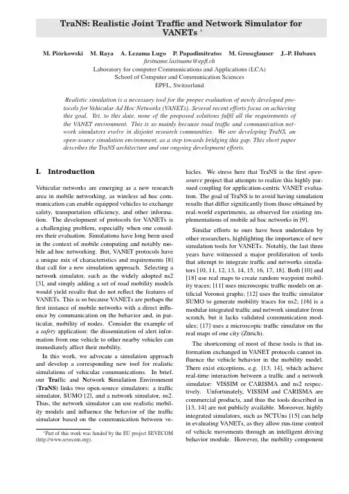
TraNS:Realistic Joint Traffic and Network Simulator forVANETs∗M.Pi´o rkowski M.Raya A.Lezama Lugo P.Papadimitratos M.Grossglauser J.-P.Hubauxfistname@epfl.chLaboratory for computer Communications and Applications(LCA)School of Computer and Communication SciencesEPFL,SwitzerlandRealistic simulation is a necessary tool for the proper evaluation of newly developed pro-tocols for Vehicular Ad Hoc Networks(VANETs).Several recent efforts focus on achievingthis goal.Yet,to this date,none of the proposed solutions fulfil all the requirements ofthe VANET environment.This is so mainly because road traffic and communication net-work simulators evolve in disjoint research communities.We are developing TraNS,anopen-source simulation environment,as a step towards bridging this gap.This short paperdescribes the TraNS architecture and our ongoing development efforts.I.IntroductionVehicular networks are emerging as a new research area in mobile networking,as wireless ad hoc com-munication can enable equipped vehicles to exchange safety,transportation efficiency,and other informa-tion.The development of protocols for V ANETs is a challenging problem,especially when one consid-ers their evaluation.Simulations have long been used in the context of mobile computing and notably mo-bile ad hoc networking.But,V ANET protocols have a unique mix of characteristics and requirements[8] that call for a new simulation approach.Selecting a network simulator,such as the widely adopted ns2 [3],and simply adding a set of road mobility models would yield results that do not reflect the features of V ANETs.This is so because V ANETs are perhaps the first instance of mobile networks with a direct influ-ence by communication on the behavior and,in par-ticular,mobility of nodes.Consider the example of a safety application:the dissemination of alert infor-mation from one vehicle to other nearby vehicles can immediately affect their mobility.In this work,we advocate a simulation approach and develop a corresponding new tool for realistic simulations of vehicular communications.In brief, our Tra ffic and N etwork S imulation Environment (TraNS)links two open-source simulators:a traffic simulator,SUMO[2],and a network simulator,ns2. Thus,the network simulator can use realistic mobil-ity models and influence the behavior of the traffic simulator based on the communication between ve-∗Part of this work was funded by the EU project SEVECOM ().hicles.We stress here that TraNS is thefirst open-source project that attempts to realize this highly pur-sued coupling for application-centric V ANET evalua-tion.The goal of TraNS is to avoid having simulation results that differ significantly from those obtained by real-world experiments,as observed for existing im-plementations of mobile ad hoc networks in[9]. Similar efforts to ours have been undertaken by other researchers,highlighting the importance of new simulation tools for V ANETs.Notably,the last three years have witnessed a major proliferation of tools that attempt to integrate traffic and networks simula-tors[10,11,12,13,14,15,16,17,18].Both[10]and [18]use real maps to create random waypoint mobil-ity traces;[11]uses microscopic traffic models on ar-tificial V oronoi graphs;[12]uses the traffic simulator SUMO to generate mobility traces for ns2;[16]is a modular integrated traffic and network simulator from scratch,but it lacks validated communication mod-ules;[17]uses a microscopic traffic simulator on the real maps of one city(Z¨u rich).The shortcoming of most of these tools is that in-formation exchanged in V ANET protocols cannot in-fluence the vehicle behavior in the mobility model. There exist exceptions,e.g.[13,14],which achieve real-time interaction between a traffic and a network simulator:VISSIM or CARISMA and ns2respec-tively.Unfortunately,VISSIM and CARISMA are commercial products,and thus the tools described in [13,14]are not publicly available.Moreover,highly integrated simulators,such as NCTUns[15]can help in evaluating V ANETs,as they allow run-time control of vehicle movements through an intelligent driving behavior module.However,the mobility component(ns2)Figure1:The network-centric mode of TraNSis highly integrated with the network simulator.This makes it hard to utilize realistic road traffic simula-tors,such as,those developed within the Intelligent Transportation Systems(ITS)community.Hence,our solution is more generic because it can combine po-tentially any realistic road traffic simulator with any network simulator.II.TraNS ArchitectureTraNS has two distinct modes of operation,each ad-dressing a specific need.Thefirst mode,which we term network-centric,can be used to evaluate,for re-alistic node mobility,V ANET communication proto-cols that do not influence in real-time the mobility of nodes.One example is user content exchange or dis-tribution(e.g.music or travel information).The sec-ond mode,termed application-centric,can be used to evaluate V ANET applications that influence node mo-bility in real-time,and thus during the traffic simula-tion runtime.Safety applications(e.g.,abrupt brak-ing,collision avoidance,etc.)are such examples.We present in detail these two architectures next.work-Centric ModeWhile operating in this mode,TraNS provides the net-work simulator with realistic mobility traces from the traffic simulator.The main component of the network-centric mode is the parser,which resides between the road traffic simulator and the network simulator.We illustrate the network-centric architecture of TraNS in Fig.1. The traffic simulator outputs a road network map and the dumpfile that contains mobility-related informa-tion about all vehicles;the parser translates this dump file into a format acceptable by the network simulator. This architecture allows for generation of the mobility traces prior to the network simulation.The current version of TraNS supports the SUMO traffic simulator[2]and the ns2network simulator [3].However,the mobility traces for ns2generatedFigure2:The application-centric mode of TraNS by TraNS can also be used by the JiST/SWANS sim-ulator[10]with some modifications.II.B.Application-Centric ModeThe second mode allows the network simulator to control the mobility of certain vehicles in simulation runtime.It is possible to modify the mobility of se-lected vehicles,depending on the simulated scenario. For example the network simulator may decide that the mobility of vehicles moving only on a specific road segment must be changed.Thus the network simulator will instruct the road traffic simulator to change their mobility attributes,while other vehicles, that are moving elsewhere,will follow the mobility process as it is controlled by the road traffic simula-tor only.We achieve this coupling by using a specific interface for interlinking road traffic and networking simulators,called TraCI[4].While working in the application-centric mode,it is possible for TraNS to perform a full-blown evaluation of V ANET applica-tions that influence vehicle’s mobility,i.e.,safety and traffic efficiency applications(e.g.SmartPark[6]). We illustrate this application-centric architecture of TraNS in Fig.2.In this mode,the mobility traces are not generated prior to network simulation,rather both simulators op-erate simultaneously.Note that in this mode no mobil-ity tracefiles are stored on a data storage device,as is the case for the network-centric mode.This becomes important,especially when large scale and long-term simulation scenarios are considered,for which mobil-ity tracefiles might become very large.The feedback loop provided by TraCI is active in this mode,thus it is possible to modify the mobility of individual vehi-cles due to information exchange within V ANET.The TraCI interface uses the atomic mobility commands, such as stop,change lane,change speed,etc.to ma-nipulate vehicle mobility.Our intuitive observation is that any complex vehicle mobility pattern,influ-enced by a V ANET application,can be broken downinto a collection of consecutive atomic mobility ac-tions performed by the driver.Thus we approximate the driver’s mobility behavior as a time sequence of the atomic mobility actions.For example,in both the Traffic Congestion Warning and the Merging Assis-tance applications proposed by the Car-to-Car Com-munication Consortium[7],vehicles may have tofirst change speed and then change lane.For the detailed description of the TraCI interface please refer to[4]. In a safety application,as it would be communi-cated to the driver,the command avoid crash can be translated into the following three consecutive mobil-ity commands:change speed(reduce),change lane and change speed(increase).The decision about when and which mobility commands should be sent to the traffic simulator are taken by the driver behavior model.Ideally the decision-making process should depend on both the information about the driving in-frastructure,such as the number of lanes on a road segment or the number of cars ahead,and the V ANET-related information.Currently,we are implement-ing a simple driver behavior model that makes deci-sions upon reception of messages exchanged between vehicles.Nevertheless,it is possible to implement more sophisticated behavioral patterns of motorists, because the TraCI interface allows for the polling of the road traffic simulator for the information related to the driving infrastructure.In our architecture,the V ANET applications are im-plemented in the network simulator.As depicted in Fig.2,the module that embodies the V ANET appli-cation logic,interacts with the driver behavior model module when it is necessary to adjust mobility at-tributes of a simulated vehicle.In both modes,the communication channel be-tween simulators is set up over a dedicated TCP/IP connection such that two separate hosts might be used to perform the simulation.In this case,TraNS needs to be installed on both hosts.TraNS also provides a graphical user interface that allows for quick and simple set up of all the required simulation parame-ters like road network topology,simulation time,TCP communication ports,dump and scenariofiles,etc. III.ConclusionIn this short paper,we present the concept and design of an integrated realistic simulation environment for V ANETs called TraNS.Our main goal is to enable de-tailed and realistic evaluation of V ANETs at network-centric,as well as application-centric levels.The cur-rent release of TraNS[1]implements the network-centric mode and provides a set of usage examples,in-cluding mobility scenarios for actual large-scale road networks.The next TraNS release will implement both the network-centric and the application-centric mode.We collaborate with other open-source simu-lation tools for V ANETs,notably[5].We also solicit contributions via[1]towards the development of an open-source simulation tool for an emerging area of mobile computing.References[1]http://trans.epfl.ch[2][3]/nsnam/ns[4]/wiki/index.php/TraCI[5]http://www.auto-nomos.de[6]http://smartpark.epfl.ch[7][8]J.Blum,A.Eskandarian,and L.Hoffman“Challenges of interve-hicle ad hoc networks,”IEEE Transactions on Intelligent Trans-portation Systems,5(4):347–351,2004.[9]W.Kiess and M.Mauve“A survey on real-world implementationsof mobile ad-hoc networks,”Ad Hoc Networks,5(3):324–339,2007.[10] D.Choffnes and F.Bustamante“An integrated mobility and trafficmodel for vehicular wireless networks,”VANET’05.[11]J.H¨a rri,M.Fiore,F.Fethi,and C.Bonnet“VanetMobiSim:gener-ating realistic mobility patterns for V ANETs,”VANET’06(Poster).[12] F.Karnadi,Z.Mo,n“Rapid Generation of Realistic MobilityModels for V ANET,”WCNC’07.[13] C.Lochert,A.Barthels,A.Cervantes,M.Mauve and M.Caliskan,“Multiple simulator interlinking environment for IVC,”VANET’05(Poster).[14]S.Eichler,B.Ostermaier,C.Schroth and T.Kosch,“Simulationof Car-to-Car Messaging:Analyzing the Impact on Road Traffic,”MASCOTS’05,507–510,2005.[15]S.Y.Wang,C.L.Chou,Y.H.Chiu,Y.S.Tseng,M.S.Hsu,Y.W.Cheng,W.L.Liu and T.W.Ho,“NCTUns4.0:An Integrated Sim-ulation Platform for Vehicular Traffic,Communication,and Net-work Researches,”WiVec’07.[16]R.Mangharam,D.Weller,D.Stancil,R.Rajkumar and J.Parikh“GrooveSim:a topography-accurate simulator for geographicrouting in vehicular networks,”VANET’05.[17]V.Naumov,R.Baumann and T.Gross“An evaluation of inter-vehicle ad hoc networks based on realistic vehicular traces,”Mo-biHoc’06.[18] A.Saha and D.Johnson“Modeling mobility for vehicular ad-hocnetworks,”VANET’04(Poster).。

基于逐元算法的地震勘探高精度谱元法数值模拟李洪建;韩立国;刘定进;巩向博【摘要】针对复杂构造地震勘探,常规正演模拟算法存在精度和计算效率低的问题,笔者研究并提出了基于逐元算法的高精度谱元法数值模拟方法.基于波动方程强、弱形式,推导二维波动方程的谱元解法,进而利用逐元算法,无需形成全局矩阵,仅对于独立的小规模单元结构进行计算,提高计算效率,减少存储空间消耗.应用基于逐元算法的高精度谱元法对复杂金属矿模型进行数值模拟,得出本方法计算精度高、数值频散小,计算效率高.%Aiming at solving the problem of low precision and low computation efficiency in conventional sim-ulation algorithm of the complex structure seismic exploration,the authors propose a high precision spectral element simulation based on element by element algorithm.Based on strong and weak forms of wave equation,the authors derivate the spectral element solution process of second-order seismic wave equation, followed by calculating the separate small-scale element structure using element by element algorithm without global matrix, which improves the computational efficiency and reduces storage space consumption.Numerical simulation of a complicated orebody model proves that this method gets high precision,small numerical dispersion and high computation efficiency.【期刊名称】《世界地质》【年(卷),期】2018(037)001【总页数】6页(P276-281)【关键词】地震勘探;谱元法;逐元法;数值模拟【作者】李洪建;韩立国;刘定进;巩向博【作者单位】中国石油化工股份有限公司石油物探技术研究院,南京211103;吉林大学地球探测科学与技术学院,长春130026;中国石油化工股份有限公司石油物探技术研究院,南京211103;吉林大学地球探测科学与技术学院,长春130026【正文语种】中文【中图分类】P631.4430 引言对于深部复杂隐伏构造地震勘探，一般采用正演数值模拟方法，结合所得到的正演反射散射特征，利用反射波成像处理技术进行地质解释和推测目标体范围。

Parallel FEM Simulation of Crack Propagation–Challenges,Status,and PerspectivesList of Authors(in alphabetical order):Bruce Carter,Chuin-Shan Chen,L.Paul Chew,Nikos Chrisochoides,Guang R.Gao,Gerd Heber,Antony R.Ingraffea,Roland Krause,Chris Myers,Demian Nave,Keshav Pingali,Paul Stodghill,Stephen Vavasis,Paul A.WawrzynekCornell Fracture Group,Rhodes Hall,Cornell University,Ithaca,NY14853CS Department,Upson Hall,Cornell University,Ithaca,NY14853CS Department,University of Notre Dame,Notre Dame,IN46556EECIS Department,University of Delaware,Newark,DE197161IntroductionUnderstanding how fractures develop in materials is crucial to many disciplines,e.g.,aeronautical engineering,mate-rial sciences,and geophysics.Fast and accurate computer simulation of crack propagation in realistic3D structures would be a valuable tool for engineers and scientists exploring the fracture process in materials.In this paper,we will describe a next generation crack propagation simulation software that aims to make this potential a reality.Within the scope of this paper,it is sufficient to think about crack propagation as a dynamic process of creating new surfaces within a solid.During the simulation,crack growth causes changes in the geometry and,sometimes,in the topology of the model.Roughly speaking,with the tools in place before the start of this project,a typical fracture analysis at a resolution of degrees of freedom,using boundary elements,would take about100hours on a state-of-the-art single processor workstation.The goal of this project is it to create a parallel environment which allows the same analysis to be done,usingfinite elements,in1hour at a resolution of degrees of freedom.In order to attain this level of performance,our system will have two features that are not found in current fracture analysis systems:Parallelism–Current trends in computer hardware suggest that in the near future,high-end engineering worksta-tions will be8-or16-way SMP“nodes”,and departmental computational servers will be built by combining a number of these nodes using a high-performance network switch.Furthermore,the performance of each processor in these nodes will continue to grow.This will happen not only because of faster clock speeds,but also becausefiner-grain parallelism will be exploited via multi-way(or superscalar)execution and multi-threading.Adaptivity–Cracks are(hopefully)very small compared with the dimension of the structure,and their growth is very dynamic in nature.Because of this,it is impossible to know a priori howfine a discretization is required to accurately predict crack growth.While it is possible to over-refine the discretization,this is undesirable,as it tends to dramatically increase the required computational resources.A better approach is to adaptively choose the discretization refinement.Initially,a coarse discretization is used,and,if this induces a large error for certain regions of the model,then the discretization is refined in those regions.The dynamic nature of crack growth and the need to do adaptive refinement make crack propagation simulation a highly irregular application.Exploiting parallelism and adaptivity presents us with three major research challenges, developing algorithms for parallel mesh generation for unstructured3D meshes with automatic element sizecontrol and provably good element quality,implementing fast and robust parallel sparse solvers,anddetermining efficient schemes for automatic,hybrid h-p refinement.To tackle the challenges of developing this system,we have assembled a multi-disciplinary and multi-institutional team that draws upon a wide-ranging pool of talent and the resources of3universities.2System OverviewFigure1gives an overview of a typical simulation.During pre-processing,a solid model is created,problem specificFigure1:Simulation loop.boundary conditions(displacements,tractions,etc.)are imposed,andflaws(cracks)are introduced.In the next step, a volume mesh is created,and(linear elasticity)equations for the displacements are formulated and solved.An error estimator determines whether the desired accuracy has been reached,or further iterations,after subsequent adaptation, are necessary.Finally,the results are fed back into a fracture analysis tool for post-processing and crack propagation.Figure1presents the simulation loop of our system in itsfinal and most advanced form.Currently,we have se-quential and parallel implementations of the outer simulation loop(i.e.,not the inner refinement loop)running with the following restrictions:currently,the parallel mesher can handle only polygonal(non-curved)boundaries,which can be handled by the sequential meshers though(see section3).We have not yet implemented unstructured h-refinement and adaptive p-refinement,although the parallel formulator can handle arbitrary p-order elements.3Geometric Modeling and Mesh GenerationThe solid modeler used in the project is called OSM.OSM,as well as the main pre-and post-processing tool, FRANC3D,is freely available from the Cornell Fracture Group’s website[12].FRANC3D-a workstation based FRacture ANalysis Code for simulating arbitrary non-planar3D crack growth-has been under development since 1987,with hydraulic fracture and crack growth in aerospace structures as the primary application targets since its inception.While there are a few3D fracture simulators available and a number of other software packages that can model cracks in3D structures,these are severely limited by the crack geometries that they can represent(typically planar elliptical or semi-elliptical only).FRANC3D differs by providing a mechanism for representing the geometry and topology of3D structures with arbitrary non-planar cracks,along with functions for1)discretizing or meshing the structure,2)attaching boundary conditions at the geometry level and allowing the mesh to inherit these values,and3) modifying the geometry to allow crack growth but with only local re-meshing required to complete the model.The simulation process is controlled by the user via a graphic user-interface,which includes windows for the display of the3D structure and a menu/dialogue-box system for interacting with the program.The creation of volume meshes for crack growth studies is quite challenging.The geometries tend to be compli-cated because of internal boundaries(cracks).The simulation requires smaller elements near each crack front in order to accurately model high stresses and curved geometry.On the other hand,larger elements might be sufficient awayfrom the crack front.There is a considerable difference between these two scales of element sizes,which amounts to three orders of magnitude in real life applications.A mesh generator must provide automatic element size control and give certain quality guarantees for elements.The mesh generators we studied so far are QMG by Steve Vavasis[15], JMESH by Joaquim Neto[11],and DMESH by Paul Chew[15].These meshers represent three different approaches: octree-algorithm based(QMG),advancing front(JMESH),and Delaunay mesh(DMESH).QMG and DMESH come with quality guarantees for elements in terms of aspect ratio.All these mesh generators are sequential and give us insight into the generation of large“engineering quality”meshes.We decided to pursue the Delaunay mesh based approachfirst for a parallel implementation,which is described in[5].Departing from traditional approaches,we simultaneously do mesh generation and partitioning in parallel.This not only eliminates most of the overhead of the traditional approach,it is almost a necessary condition to do crack growth simulations at this scale,where it is not always possible or too expensive to keep up with the geometry changes by doing structured h-refinement.The implementation is a parallelization of the so-called Bowyer-Watson(see the references in[5])algorithm:given an initial Delaunay triangulation,we add a new point to the mesh,determine the simplex containing this point and the point’s cavity(the union of simplices with non-empty circumspheres),and,fi-nally,retriangulate this cavity.One of the challenges for a parallel implementation is that this cavity might extend across several submeshes(and processors).What looks like a problem,turns out to be the key element in unifying mesh generation and partitioning:the newly created elements,together with an adequate cost function,are the best candidates to do the“partitioning on thefly”.We compared our results with Chaco and MeTis in terms of equidistri-bution of elements,relative quality of mesh separators,data migration,I/O,and total performance.Table1shows a runtime comparison between ParMeTis with PartGeomKway(PPGK)and,our implementation,called SMGP,on16 processors of an IBM SP2for meshes of up to2000K elements.The numbers behind SMGP refer to different cost functions used in driving the partitioning[5].Mesh Size PPGK SMGP0SMGP1SMGP2SMGP3200K9042424242500K215658764621000K4399716091942000K1232133310110135Table1:Total run time in seconds on16processors.4Equation Solving and PreconditioningWe chose PETSc[2,14]as the basis for our equation solver subsystem.PETSc provides a number of Krylov space solvers,and a number of widely-used preconditioners.We have augmented the basic library with third party packages, including BlockSolve95[8]and the Barnard’s SPAI[3].In addition,we have implemented a parallel version of the Global Extraction Element-By-Element(GEBE)preconditioner[7](which is unrelated to the EBE preconditioner of Winget and Hughes),and added it to the collection using PETSc’s extension mechanisms.The central idea of GEBE is to extract subblocks of the global stiffness matrix associated with elements and invert them,which is highly parallel.The ICC preconditioner is frequently used in practice,and is considered to be a good preconditioner for many elasticity problems.However,we were concerned that it would not scale well to the large number of processors required for ourfinal system.We believed that GEBE would provide a more scalable implementation,and we hoped that it would converge nearly as well as ICC.In order to test our hypothesis,we ran several experiments on the Cornell Theory Center SP-2.The preliminary performance results for the gear2and tee2models are shown in Tables2and3,respectively.(gear2is a model of a power transmission gear with a crack in one of its teeth.tee2is a model of a T steel profile).For each model,we ran the Conjugant Gradient solver with both BlockSolve95’s ICC preconditioner and our own parallel implementation of GEBE on8to64processors.(The iteration counts in Tables2and3correspond to a reduction of the residualerror,which is completely academic at this point.)The experimental results confirm our hypothesis: GEBE converges nearly as quickly as ICC for the problems that we tested.Our naive GEBE implementation scales much better than BlockSolve95’s sophisticated ICC implementation.Prec.Nodes Prec Time Per Iters.TypeTime(s)Iteration (s)ICC817.080.2416GEBE89.430.19487ICC1615.470.27422GEBE16 6.710.11486ICC328.510.32539GEBE32 3.730.08485ICC6411.000.28417GEBE 64 4.740.07485Table 2:Gear2(79,656unknowns)Prec.Nodes Prec Time Per Iters.Type Time(s)Iteration (s)ICC 3230.000.292109GEBE 3235.700.212421ICC 6423.600.292317GEBE 647.600.122418Table 3:Tee2(319,994unknowns)5AdaptivityUnderstanding the cost and impact of the different adaptivity options is the central point in our current activities.We are in the process of integrating the structured (hierarchical)h-re finement into the parallel testbed,and the final version of this paper will contain more results on that.Our implementation follows the approach of Biswas and Oliker [4]and currently handles tetrahedra,while allowing enough flexibility for an extension to non-tetrahedral element types.Error Estimation and Adaptive Strategies.For relatively simple,two-dimensional problems,stress intensity factors can be computed to an accuracy suf ficient for engineering purposes with little mesh re finement by proper use of sin-gularly enriched elements.There are many situations though when functionals other than stress intensity factors are of interest or when the singularity of the solution is not known a priori .In any case the engineer should be able to evaluate whether the data of interest have converged to some level of accuracy considered appropriate for the compu-tation.It is generally suf ficient to show,that the data of interest are converging sequences with respect to increasing degrees of freedom.Adaptive finite element methods are the most ef ficient way to achieve this goal and at the same time they are able to provide estimates of the remaining discretization error.We de fine the error of the finite elementsolutionasand a possible measure for the discretization error is the energynorm,Following an idea of Babu ˇs ka and Miller [1]the error estimator introduced by Kelly et.al.[9,6]is derived by inserting the finite element solution into the original differential equation system and calculating a norm of the residual using interpolation estimates.An error indicator computable from local results of one element of the finite element solution is then derived and the corresponding error estimator is computed by summing the contribution of the error indicators over the entire domain.The error indicator is computed with a contribution from the interior residual of the element and a contribution of the stress jumps on the faces of an element.Details on the computation of the error estimator from the finite element solution can be found in [10].Control of a Mesh Generator.For a sequence of adaptively re fined and quasi optimal meshes,the rate of conver-gence is independent of the smoothness of the exact solution.A mesh is called quasi optimal if the error associated with each element is nearly the same.The goal of an adaptive finite element algorithm is to generate a sequence of quasi optimal meshes by equilibrating the estimated error until a prescribed accuracy criterion is reached.Starting from an initial mesh,error indicators and the error estimator are computed in the post-processing step of the solutionphase.The idea is then to compute for each element the new elementsizefrom the estimated error,the present elementsize and the expected rate of convergence.6Future WorkThe main focus of our future work will be on improving the performance of the existing system.The Cornell Fracture Group is continuously extending our test-suite with new real world problems.We are considering introducing special elements at the crack tip,and non-tetrahedral elements (hexes,prisms,pyramids)elsewhere.The linear solver,after proving its robustness,will be wrapped into a Newton-type solver for nonlinear problems.Among the newly introduced test problems are some that can be made arbitrarily ill-conditioned (long thin plate or tube models with cracks in them)in order to push the iterative methods to their limits.We are exploring new precon-ditioners (e.g.,support tree preconditioning),and multigrid,as well as sparse direct solvers,to make our environmentmore effective and robust.We have not done yet any specific performance tuning,like locality optimization.This is not only highly platform dependent,but also has to be put in perspective to the forthcoming runtime optimizations,like dynamic load balancing. We are following with interest the growing importance of latency tolerant architectures in the form of multithreading and exploring for which parts of the project multithreaded architectures are the most beneficial.Finally,there is a port of our code base to the new256node NT cluster at the Cornell Theory Center underway. 7ConclusionsAt present,our project can claim two major contributions.Thefirst is our parallel mesher/partition,which is thefirst practical implementation of its kind with quality guarantees.This technology makes it possible,for thefirst time,to fully automatically solve problems using unstructured h-refinement in a parallel setting.The second major contribution is to show that GEBE outperforms ICC,at least for our problem class.We have shown that,not only does GEBE converge almost as quickly as ICC,it is much more scalable in a parallel setting than ICC.We believe that GEBE,not ICC,is the yardstick against which other parallel preconditioners should be measured.Andfinally,ourfirst experimants indicate that we should be able to meet our project’s performance goals.We are confident that,as we run our system on larger and faster machines,as we further optimize each of the subsystems,and as we incorporate adaptive h-and p-refinement,we will reach our performance goals.References[1]I.Babuˇs ka and ler,“A-posteriori error estimates and adaptive techniques for thefinite element method,”Technical Report Tech.Note BN–968,University of Maryland,Inst.for Physics,Sci.and Tech.,1981.[2]S.Balay,W.D.Gropp,L.Curfman McInnes,and B.F.Smith,“Efficient management of parallelism in object-oriented numerical software libaries”,In E.Arge,A.M.Bruaset,and ngtangen,editors,Modern Software Tools in Scientific Computing,Birkhauser Press,1997.[3]S.T.Barnard and R.Clay,“A portable MPI implementation of the SPAI preconditioner in ISIS++”,Eighth SIAMConference for Parallel Processing for Scientific Computing,March1997.[4]R.Biswas and L.Oliker,“A new procedure for dynamic adaption of three-dimensional unstructured grids”,AppliedNumerical Mathematics,13:437–452,1994.[5]N.Chrisochoides and D.Nave,“Simultaneous mesh generation and partitioning for Delaunay meshes”,In8thInt’l.Meshing Roundtable,1999.[6]J.P.de S.R.Gago,D.W.Kelly,O.C.Zienkiewicz,and I.Babuˇs ka,“A posteriori error analysis and adaptive processesin thefinite element method:Part II–Adaptive mesh refinement”,International Journal for Numerical Methods in Engineering,19:1621–1656,1983.[7]I.Hladik,M.B.Reed,and G.Swoboda,“Robust preconditioners for linear elasticity FEM analyses”,InternationalJournal for Numerical Methods in Engineering,40:2109–2127,1997.[8]M.T.Jones and P.E.Plassmann,“Blocksolve95users manual:Scalable library software for the parallel solution ofsparse linear systems”,Technical Report ANL-95/48,Argonne National Laboratory,December1995.[9]D.W.Kelly,J.P.de S.R.Gago,O.C.Zienkiewicz,and I.Babuˇs ka,“A posteriori error analysis and adaptive processesin thefinite element method:Part I–Error analysis”,International Journal for Numerical Methods in Engineering, 19:1593–1619,1983.[10]R.Krause,“Multiscale Computations with a Combined-and-Version of the Finite Element Method”,PhDthesis,Universit¨a t Dortmund,1996.[11]o et al.,“An Algorithm for Three-Dimensional Mesh Generation for Arbitrary Regions with Cracks”,submitted for publication.[12]/.[13]/People/chew/chew.html.[14]/petsc/index.html.[15]/vavasis/vavasis.html.。

模拟蜜蜂声音的英语作文Title: Buzzing with Life: Simulating the Sound of Bees。

In the natural world, few sounds evoke the sense of vitality and industry quite like the buzzing of bees. From the gentle hum of foragers gathering nectar to the frenetic buzz of a hive in full activity, the sound of bees is a symphony of life. Capturing and simulating this sound inthe realm of technology is a fascinating endeavor, one that requires an understanding of both the mechanics of beeflight and the nuances of sound production.To simulate the sound of bees authentically, we mustfirst delve into the physics of their flight. Bees generate the buzzing sound primarily through the rapid movement of their wings. Unlike many other insects, bees have two setsof wings that beat in unison, creating a distinctivebuzzing sound frequency. The frequency of this buzzingvaries depending on the size and species of the bee,ranging from around 200 to 400 Hz for honeybees, forinstance.Next, we must consider the environment in which bees produce their buzzing. The buzzing of bees is not just a product of their wing movement but is also influenced by the surrounding air and objects. For example, bees may produce a louder buzzing sound when flying close to surfaces due to the amplification effect of nearby structures. Additionally, factors such as temperature and humidity can affect the propagation of sound waves, further shaping the acoustic signature of bees in flight.In simulating the sound of bees, we can employ various techniques borrowed from the field of audio engineering and computer science. One approach is to use recordings of actual bee buzzing as a basis for generating synthetic sounds. By analyzing the frequency spectrum and amplitude envelope of these recordings, we can create algorithms that replicate the buzzing patterns of bees with remarkable accuracy. These algorithms can then be implemented in software or electronic devices to produce lifelike bee sounds.Another approach involves the use of physical models to simulate the behavior of bee wings and the surrounding air. By modeling the aerodynamics of bee flight and the acoustic properties of the environment, we can simulate the buzzing sound in real-time. This approach offers greaterflexibility and realism, allowing us to simulate a wide range of bee behaviors and environmental conditions.Furthermore, advances in artificial intelligence and machine learning hold promise for enhancing the realism of bee sound simulation. By training AI models on vast amounts of bee flight data, we can teach them to generate highly realistic buzzing sounds based on various parameters such as bee species, flight speed, and environmental factors. This approach not only improves the fidelity of bee sound simulation but also opens up possibilities for interactive and adaptive simulations that respond to changes in the virtual environment.In conclusion, simulating the sound of bees is a multifaceted endeavor that combines insights from biology,physics, engineering, and computer science. Byunderstanding the underlying mechanisms of bee flight and sound production, and leveraging cutting-edge technologies, we can create immersive simulations that capture the essence of these remarkable insects. Whether foreducational purposes, entertainment, or scientific research, simulated bee sounds offer a window into the intricateworld of these vital pollinators. Buzzing with life, they remind us of the beauty and complexity of the natural world.。

References[1]A.Bazzi, B.Masini, A.Zanella, G.Pasolini, Virtual road side units for georouting in VANETs, in: Proceedings of the International Conferenceon Connected Vehicles & Expo (ICCVE,2014),2014.[2]NHSTA web page. , (accessedJune2015).[3]R.Uzcategui, G.Acosta-Marum, WAVE: atutorial, IEEE Commun. Mag. 47(5) (2009)126–133, doi: 10.1109/MCOM.2009.4939288.[4]A.Bazzi, B.Masini, G.Pasolini, V2V and V2R for cellular resources saving in vehicular applications, in: Proceedings of the IEEE Wireless Communications and Networking Conference (WCNC), 2012, pp. 3199–3203,doi:10.1109/WCNC.2012.6214358.[5]R.Ganti, F.Ye, H.Lei, Mobile crowdsensing: current state and future challenges, IEEE Commun.Mag.49(11)(2011)32–39,doi: 10.1109/MCOM.2011.6069707.[6]H.Ma, D.Zhao, P.Yuan, Opportunities in mobile crowd sensing, IEEE Commun.Mag.52(8) (2014)29–35,doi:10.1109/MCOM.2014.6871666.[7]X.Yu, H.Zhao, L.Zhang, S.Wu, B.Krishnamachari, V.Li, Cooperative sensing and compression in vehicular sensor networks for urban monitoring, in: Proceedings of the IEEE International Conference on Communications (ICC),2010,pp.1–5,doi:10.1109/ICC.2010.5502562.[8]A.R.Al-Ali, I.Zualkernan, F.Aloul, Amobile GPRS-sensors array for air pollution monitoring, IEEE Sens. J. 10(10)(2010)1666–1671,doi:10.1109/JSEN.2010.2045890.[9]A.Bazzi, B.Masini, O.Andrisano, On the frequent acquisition of small data through RACH in UMTS for ITS applications, IEEE Trans. Veh.Technol.60(7)(2011)2914–2926,doi:10.1109/TVT.2011.2160211.[10]C.Lochert, B.Scheuermann, C.Wewetzer, A.Luebke, M.Mauve, Data aggregation and roadside unit placement for a VANET traffic information system, in: Proceedings of the Fifth ACM International Workshopon Vehicular Inter-Networking, in: VANET’08, ACM, NewYork, NY, USA, 2008, pp.58–65, doi:10.1145/1410043.1410054.[11]B.Aslam, F.Amjad, C.Zou, Optimal roadside units placement in urban areas for vehicular networks, in: Proceedings of the IEEE Symposium on Computers and Communications (ISCC), 2012, pp. 000423–000429,doi:10.1109/ISCC.2012.6249333.[12]N.Benamar, K.D.Singh, M.Benamar, D.E.Ouadghiri, J.-M.Bonnin, Routing protocols in vehicular delay tolerant networks: a comprehensive survey, Comput. Commun. 48(0) (2014)141–158, doi:10.1016/com.2014.03.024.[13]Z.Taysi, A.Yavuz, Routing protocols for geonet: asurvey, IEEE Trans. Intell. Transp. Syst. 13(2) (2012)939–954,doi:10.1109/TITS.2012.2183637.[14]M.Mauve, J.Widmer, H.Hartenstein, A survey on position-basedrouting in mobile ad hoc networks, Network, IEEE15 (6) (2001)30–39,doi:10.1109/65.967595.[15]B.Karp, H.T.Kung, GPSR: greedy perimeter stateless routing for wireless networks, in: Proceedings of the 6th Annual International Conference on Mobile Computing and Networking (MobiCom’00),ACM,NewYork,NY,USA,2000,pp.243–254,doi:10.1145/345910.345953.[16]C.Lochert, M.Mauve, H.Füssler, H.Hartenstein, Geographic routing in city scenarios, SIGMOBILE mun. Rev. 9(1)(2005)69–72,doi:10.1145/1055959.1055970.[17]U.Lee, E.Magistretti, B.Zhou, M.Gerla, P.Bellavista, A.Corradi, Efficient data harvesting in mobile sensor platforms, in: Proceedings of the Fourth Annual IEEE International Conference on Pervasive Computing and Communications Workshops (PerCom), 2006, pp.5–356,doi:10.1109/PERCOMW.2006.47.[18]ert, M.Cetin, Queue length estimation from probe vehicle location and the impacts of sample size, Eur.J.Oper.Res.197(1)(2009)196–202,doi:10.1016/j.ejor.2008.06.024.[19]R.Stanica, M.Fiore, F.Malandrino, Offloading floating car data,in :Proceedings of the 14th IEEE International Symposium and Workshops on a World of Wireless, Mobile and Multimedia Networks(WoWMoM),2013,pp.1–9,doi:10.1109/WoWMoM.2013.6583391.[20]U.Lee, M.Gerla, A survey of urban vehicular sensing platforms, w.54(4)(2010)527–544,doi:10.1016/net.2009.07.011.[21]B.Masini, L.Zuliani, O.Andrisano, On the effectiveness of a GPRS based intelligent transportation system in a realistic scenario, in: Proceedings of the IEEE 63rd Vehicular Technology Conference(VTC2006-Spring),6,2006,pp.29973001, doi:10.1109/VETECS.2006.1683418.[22]I.Leontiadis, G.Marfia, D.Mack, G.Pau, C.Mascolo, M.Gerla, On the effectiveness of an opportunistic traffic management system for vehicular networks, IEEE Trans.Intell.Transp.Syst.12(4)(2011)1537–1548,doi:10.1109/TITS.2011.2161469.[23]C.deFabritiis, R.Ragona, G.Valenti, Traffic estimation and prediction based on real time floating car data, in: Proceedings of the 11th International IEEE Conference on Intelligent Transportation Systems(ITSC),2008,pp.197–203,doi:10.1109/ITSC.2008.4732534.[24]A.Skordylis, N.Trigoni, Efficient data propagation in traffic-monitoring vehicular networks, IEEE Trans.Intell.Transp.Syst.12(3)(2011)680694,doi:10.1109/TITS.2011.2159857.[25]A.Bazzi, B.M.Masini, A.Zanella, G.Pasolini, {IEEE} 802.11p for cellular offloading in vehicular sensor networks, Comput. Commun.60(2015)97–108,doi:10.1016/com.2015.01.012. [26]F.Li, Y.Wang, Routing in vehicular ad hoc networks: asurvey,IEEEVeh. Technol. Mag. 2(2)(2007)1222,doi:10.1109/MVT.2007.912927.[27]V.Naumov, T.Gross, Connectivity-aware routing (CAR) in vehicular ad-hoc networks, in: Proceedings of the 26th IEEE International Conference on Computer Communications (INFOCOM), 2007,pp.1919–1927,doi:10.1109/INFCOM.2007.223.[28]J.Haerri, F.Filali, C.Bonnet, Performance comparison of AODV and OLSR in VANETs urban environments under realistic mobility patterns, in:Proceedings of the 5th IFIP Mediterranean Ad-Hoc Networking Workshop (Med-Hoc-Net-2006), Lipari,Italy,2006.[29]A.Vahdat, D.Becker, etal., Epidemic routing for partially connected ad hoc networks, Technical Report CS-200006, DukeUniversity, Durham, NorthCarolina,2000.[30]T.Spyropoulos, K.Psounis, C.S.Raghavendra, Sprayandwait: anefficient routing scheme for intermittently connected mobile networks,in: Proceedings of the 2005 ACM SIGCOMM Workshop on Delaytolerant Networking(WDTN’05),ACM,NewYork,NY,USA,2005,pp.252259,doi:10.1145/1080139.1080143. [31]Y.Xiang, Z.Liu, R.Liu, W.Sun, W.Wang, GeoSVR: a map-based stateless VANET routing, Ad HocNetw.11(7)(2013)2125–2135, doi:10.1016/j.adhoc.2012.02.015.[32]K.Mershad, H.Artail, M.Gerla, ROAMER: roadside units as message routers in VANETs, Ad Hoc Netw.10(3)(2012)479–496,doi:10.1016/j.adhoc.2011.09.001.[33]S.Ahmed, S.S.Kanere, SKVR: Scalable knowledge-based routing architecture for public transport networks, in: Proceedings of the 3rd International Workshop on Vehicular Ad Hoc Networks(VANET’06),ACM,NewYork,NY,USA,2006,pp.92–93,doi:10.1145/1161064.1161082.[34]Q.Yuan, I.Cardei, J.Wu, An efficient prediction-based routing in disruption-tolerant networks ,IEEE Trans. Parallel Distrib.Syst.23(1)(2012)19–31,doi:10.1109/TPDS.2011.140.[35]C.Lochert, H.Hartenstein, J.Tian, H.Fussler, D.Hermann, M.Mauve, A routing strategy for vehicular ad hoc networks in city environments, in: Intelligent Vehicles Symposium,2003.Proceedings.IEEE,2003,pp.156–161,doi:10.1109/IVS.2003.1212901.[36]T.Camp, J.Boleng, L.Wilcox, Location information services in mobile ad hoc networks, in: Proceedings of IEEE International Conference on Communications (ICC),5,2002,pp.3318–3324, doi:10.1109/ICC.2002.997446.[37]J.Bernsen, D.Manivannan, Unicast routing protocols for vehicular ad hoc networks: acritical comparison and classification, Pervasive Mob.Comput.5(1)(2009)1–18,doi:10.1016/j.pmcj.2008.09.001.[38]K.Lee, J.Haerri, U.Lee, M.Gerla, Enhanced perimeter routing for geographic forwarding protocols in urban vehicular scenarios, in: Proceedings of IEEE Globecom Workshops,2007,pp.1–10,doi:10.1109/GLOCOMW.2007.4437832.[39]A.Bazzi, G.Pasolini, C.Gambetti, SHINE: simulation platform for heterogeneous interworking networks, in: Proceedings of IEEE International Conference on Communications(ICC’06),12,2006,pp.5534–5539,doi:10.1109/ICC.2006.255543.[40]A.Toppan, A.Bazzi, P.Toppan, B.Masini, O.Andrisano, Architecture of a simulation platform for the smart navigation service investigation, in:Proceedings of the 6th International IEEE Conference on Wireless and Mobile Computing, Networking and Communications(WiMob),2010,pp.548-554,doi:10.1109/WIMOB.2010.5645014.[41]SHINE web page. r.it/people/bazzi/SHINE.html,(accessedJune2015).[42]C.Campolo, A.Molinaro, Multichannel communications in vehicular ad hoc networks: a survey,IEEE Commun.Mag.51(5)(2013)158–169,doi:10.1109/MCOM.2013.6515061.[43]S.Uppoor, O.Trullols-Cruces, M.Fiore, J.Barcelo-Ordinas, Generation and analysis of a large-scale urban vehicular mobility dataset, IEEE put.99(PP)(2013),doi:10.1109/TMC.2013.27.[44]A.Benslimane, S.Barghi, C.Assi, An efficient routing protocol for connecting vehicular networks to the internet, Pervasive Mob. Comput.7(1)(2011)98–113,doi:10.1016/j.pmcj.2010.09.002.[45]J.-J.Chang, Y.-H.Li, W.Liao, I.-C.Chang, Intersection-based routing for urban vehicular communications with traffic-light considerations, IEEEmun19(1)(2012)82–88,doi:10.1109/MWC.2012.6155880.[46]F.Martinez, C.-K.Toh, J.-C.Cano, C.Calafate, P.Manzoni, Realistic radio propagation models (RPMs) for VANET simulations, in: Proceedings of IEEE Wireless Communication sand Networking Conference (WCNC),2009,pp.1–6,doi:10.1109/WCNC.2009.4917932.[47]L.Cheng, B.Henty, D.Stancil, F.Bai, P.Mudalige, Mobile vehicle-to-vehicle narrow-band channel measurement and characterization of the 5.9 GHz dedicated short range communication (DSRC)frequencyband, IEEE J. Sel. AreasCommun.25(8)(2007)1501–1516,doi:10.1109/JSAC.2007.071002.引用[1] A.Bazzi, B.Masini, A.Zanella, G.Pasolini, 由、虚拟路边单元在VANETs georouting:《国际会议上连接车辆&世博会(ICCVE,2014),2014。