Differential Trace Design Rules
Truth vs Fiction
Truth vs Fiction
Truth vs Fiction
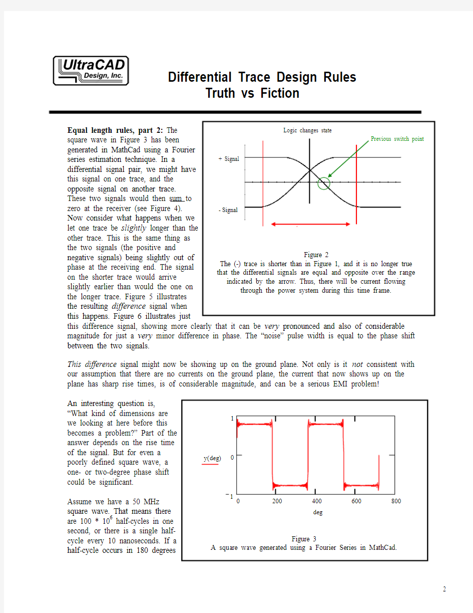
Truth vs Fiction Array (half of a 360 degree complete cycle), and if propagation time is 6” per nanosecond in FR4, then one degree phase shift equates to 333 mils distance. If we set one degree as our threshold, (which might be too much!) then the corresponding offsets would be:
Frequency (MHz) Offset (mils, or thousandth in.)
50 333
500 33
5 GHz 3
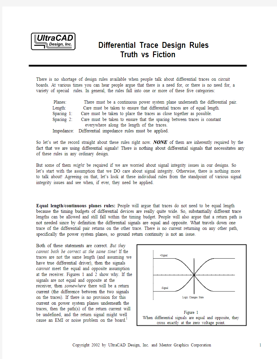
Conclusion: The equal length design rule is important IF the signal equal-and-opposite assumption is important. The signal equal-and-opposite assumption is important if we are worried about EMI or if we require discontinuities in the power system grounds between two circuits.
Close together rule, part 1: It is generally understood that EMI is related to loop area.2 The loop area is defined as the area between the signal path and its return path. On differential traces, the signal is on one trace and the return is on the other trace. So the loop area is a function of how close the traces are routed together.
If we are concerned about EMI, we must route the traces close together. The more closely we route them to each other, the smaller the loop area will be and the less EMI that will be generated.
Close together rule, part 2: One of the primary advantages of differential signals is the signal-to-noise ratio improvement that is obtained. Since the signal is one polarity on one trace and the other polarity on the other trace, the resulting signal at the receiving device is twice what the single-ended signal would be. An additional advantage is that the receiving circuits are designed so that they are highly sensitive to the difference in signal level between the two traces, but highly insensitive to shifts in signal level that occur
on both traces. This is normally called common mode rejection at the receiving device.
Truth vs Fiction
In order to have good common mode noise rejection, it is important that any noise that is present affects the signals on both traces equally. That is, if noise is coupled into one trace, an equal amount of noise must be coupled into the other trace. Then the common mode rejection capability of the receiving circuit will reject the noise. But if noise is coupled into one trace more strongly than into the other trace, the noise will appear as a differential mode signal to the receiver and be amplified.
The way to ensure that any noise is coupled equally into both traces is to route the two traces very close together. Then they will both be in the same noise environment.
Conclusion: The close together rule is important IF we are worried about EMI or IF we are worried about common mode rejection of noise that has been coupled into our traces.
Continuous plane rule, part 2: Assuming signal integrity issues are important, we are probably worried about signal reflections at the end of traces. If we are worried about reflections, then we need impedance controlled traces. If we need impedance controlled traces, then it is almost axiomatic that we need continuous planes underneath those traces.3 Otherwise, impedance control is very difficult to achieve and impedance discontinuities will develop.
Constant spacing rule: When two traces are routed close together, there is coupling between them. Ordinarily we call that crosstalk. But in the very special case of differential signals, we don’t refer to it as crosstalk, and there is no negative implication to this coupling. The very special case derives from the fact that the two differential signals (in an ordinary case referred to as the aggressor and the victim signals) are perfectly correlated. One is the exact inverse of the other.
There is a consequence of this coupling. The consequence is that the resulting impedance of the trace reduces from its single-ended value.4 The normal expression for the resulting impedance is Z = Zo – Z12
where Z12 represents the effects of the coupling.
The coupling is a function of the spacing. Traces spaced very far apart have little or no effective coupling, and their characteristic impedance is simply Zo. Traces placed very close together have some degree of coupling, and therefore lower impedance. If we are concerned about using impedance controlled traces, then we are also concerned about having a constant impedance everywhere along the trace. Otherwise, the resulting impedance discontinuities may cause reflections.
Conclusion: If we are using controlled impedance traces, then it is important that the separation between traces remain constant everywhere along their length. (Note that this conclusion says nothing about how closely they should be spaced. That conclusion derives from EMI and common mode noise rejection considerations.)
Differential impedance rule: The so-called differential impedance rule simply says we must calculate a differential impedance for proper trace termination if differential signals are routed close together. There is nothing magical about differential impedance. We would not have to use differential impedance calculations if traces were routed widely apart. But:
Truth vs Fiction
IF signal reflections are an issue, so that we need impedance controlled traces, and
IF the traces need to be routed close together for EMI and/or common mode rejection reasons, consequence is that differential calculations become necessary.
the
THEN
Summary: There is nothing about differential signals that requires special routing rules unless we are concerned about signal integrity issues. Then, certain signal integrity issues result in certain design guidelines. Some of these guidelines have consequences that lead to additional design rules that might not have been necessary otherwise.
___________________
Footnotes:
1. For a discussion of planes and problems associated with plane discontinuities, see Brooks, “Splitting
Planes for Speed and Power,” available from https://www.doczj.com/doc/6117670790.html,.
2. See Brooks, “Loop Areas, Close ‘Em Tight,” Printed Circuit Design Magazine, January, 1999,
available from https://www.doczj.com/doc/6117670790.html,.
3. There are a variety of articles and publications regarding trace impedance guidelines. For example
see “PCB Impedance Control: Formulas and Resources,” March, 1998, “Impedance Terminations: What’s the Value?” March, 1999; and “What Is Characteristic Impedance?” by Eric Bogatin,
January, 2000, p. 18, all from Printed Circuit Design Magazine. For embedded microstrip formulas see “Embedded Microstrip,” Printed Circuit Design, February, 2000. All articles (except Bogatin’s) are reprinted on UltraCAD’s web site.
4. See Brooks, “Differential Impedance, What’s the Difference?” Printed Circuit Design Magazine,
August, 1998, available from https://www.doczj.com/doc/6117670790.html,,
About the author:
Douglas Brooks has a B.S and an M.S in Electrical Engineering from Stanford University and a
PhD from the University of Washington. During his career has held positions in engineering,
marketing, and general management with such companies as Hughes Aircraft, Texas Instruments
and ELDEC.
Brooks has owned his own manufacturing company and he formed UltraCAD Design Inc. in 1992.
UltraCAD is a service bureau in Bellevue, WA, that specializes in large, complex, high-density,
high-speed designs, primarily in the video and data processing industries. Brooks has written numerous articles through the years, including articles and a column for Printed Circuit Design Magazine, and has been a frequent seminar leader at PCB Design Conferences. His primary objective in his speaking and writing has been to make complex issues easily understandable to those without a technical background. You can visit his web page at