
第四章 数值计算
与符号计算相比,数值计算在科研和工程中的应用更为广泛。MATLAB 也正是凭借其卓越的数值计算能力而称雄世界。随着科研领域、工程实践的数字化进程的深入,具有数字化本质的数值计算就显得愈益重要。
较之十年、二十年前,在计算机软硬件的支持下当今人们所能拥有的计算能力已经得到了巨大的提升。这就自然地激发了人们从新的计算能力出发去学习、理解概念的欲望,鼓舞了人们用新计算能力试探解决实际问题的雄心。
鉴于当今高校本科教学偏重符号计算和便于手算简单示例的实际,也出于帮助读者克服对数值计算生疏感的考虑,本章在内容安排上仍从“微积分”开始。这一方面与第2章符号计算相呼应,另方面通过“微积分”说明数值计算离散本质的微观和宏观影响。
为便于读者学习,本章内容的展开脉络基本上沿循高校数学教程,而内容深度力求控制在高校本科水平。考虑到知识的跳跃和交叉,本书对重要概念、算式、指令进行了尽可能完整地说明。
数值微积分
近似数值极限及导数
【例4.1-1】设x x x x f sin 2cos 1)(1-=
,x
x
x f sin )(2=,试用机器零阈值eps 替代理论0计算极限
)(lim )0(10
1x f L x →=,)(lim )0(20
2x f L x →=。
%不可信的“极限的数值近似计算” x=eps;
L1=(1-cos(2*x))/(x*sin(x)), L2=sin(x)/x,
L1 = 0 L2 =
1
%正确的“极限的符号计算”
syms t
f1=(1-cos(2*t))/(t*sin(t)); f2=sin(t)/t;
Ls1=limit(f1,t,0) Ls2=limit(f2,t,0)
Ls1 = 2
Ls2 = 1
说明:不能随便使用数值计算方法求极限!!因为数值计算的最小精度为eps ,不等价于数学上的无穷小。
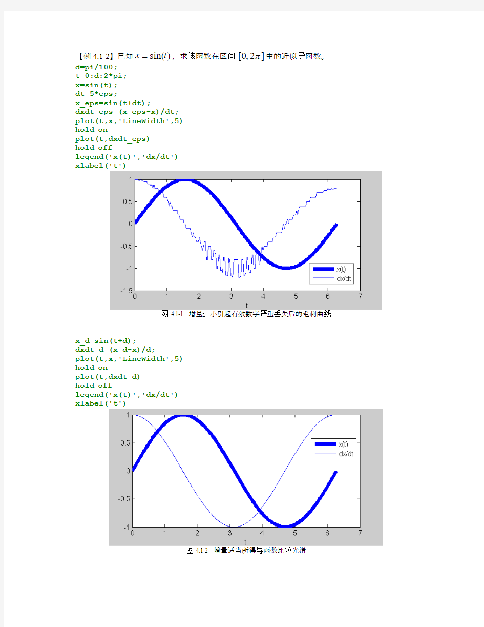
【例4.1-2】已知)sin(t x =,求该函数在区间 ]2 ,0[π中的近似导函数。 d=pi/100; t=0:d:2*pi; x=sin(t); dt=5*eps; x_eps=sin(t+dt);
dxdt_eps=(x_eps-x)/dt; plot(t,x,'LineWidth',5) hold on
plot(t,dxdt_eps) hold off
legend('x(t)','dx/dt') xlabel('t')
图 4.1-1 增量过小引起有效数字严重丢失后的毛刺曲线
x_d=sin(t+d);
dxdt_d=(x_d-x)/d; plot(t,x,'LineWidth',5) hold on
plot(t,dxdt_d) hold off
legend('x(t)','dx/dt') xlabel('t')
图 4.1-2 增量适当所得导函数比较光滑
说明:
(1)数值导数结果受到计算中的有限精度困扰,当自变量增量太小,则函数值过于接近,导致计算精度变差。
(2)不要随便使用数值方法计算导数。
此处关于diff(),gradient()的说明见PPT.
a=1:10
diffa = diff(a)
grada=gradient(a)
a =
1 2 3 4 5 6 7 8 9 10
diffa =
1 1 1 1 1 1 1 1 1
grada =
1 1 1 1 1 1 1 1 1 1
b=[1:10;11:20]
b =
1 2 3 4 5 6 7 8 9 10
11 12 13 14 15 16 17 18 19 20
diffb = diff(b)
gradb=gradient(b)
[gradbx,gradby]=gradient(b)
diffb =
10 10 10 10 10 10 10 10 10 10
gradb =
1 1 1 1 1 1 1 1 1 1
1 1 1 1 1 1 1 1 1 1
gradbx =
1 1 1 1 1 1 1 1 1 1
1 1 1 1 1 1 1 1 1 1
gradby =
10 10 10 10 10 10 10 10 10 10
10 10 10 10 10 10 10 10 10 10
【例4.1-3】已知)sin(t x =,采用diff 和gradient 计算该函数在区间 ]2 ,0[π中的近似导函数。。 clf
d=pi/100; t=0:d:2*pi; x=sin(t);
dxdt_diff=diff(x)/d; %近似导数 dxdt_grad=gradient(x)/d; %近似导数
subplot(1,2,1) plot(t,x,'b') hold on
plot(t,dxdt_grad,'m','LineWidth',8)
plot(t(1:end-1),dxdt_diff,'.k','MarkerSize',8) %这里dxdt_diff 只有end-1 % 个元素 axis([0,2*pi,-1.1,1.1]) title('[0, 2\pi]')
legend('x(t)','dxdt_{grad}','dxdt_{diff}','Location','North') xlabel('t'),box off hold off
subplot(1,2,2)
kk=(length(t)-10):length(t); %选中最后的10个数据点 hold on
plot(t(kk),dxdt_grad(kk),'om','MarkerSize',8)
plot(t(kk-1),dxdt_diff(kk-1),'.k','MarkerSize',8) %dxdt_diff 只有end-1个 title('[end-10, end]')
legend('dxdt_{grad}','dxdt_{diff}','Location','SouthEast') xlabel('t'),box off hold off
图 4.1-3 diff 和gradient 求数值近似导数的异同比较
说明:
(1)宏观上,diff和gradient所求近似导数大体相同;
(2)diff和gradient不仅在数值上有差异,而且diff没有给出最后一个点的导数。
4.1.2数值求和与近似数值积分
补充例子:
1、cumsum(X)的用法
CUMSUM Cumulative sum of elements.
For vectors, CUMSUM(X) is a vector containing the cumulative sum of
the elements of X. For matrices, CUMSUM(X) is a matrix the same size
as X containing the cumulative sums over each column. For N-D
arrays, CUMSUM(X) operates along the first non-singleton dimension.
cumsum用来计算累计求和。
如果X是向量,cumsum(X)是一个向量,包括X所有元素的累积求和结果;
如果X是矩阵,cumsum(X)是一个和X相同大小的矩阵,包括X按列累积求和结果;如果X是N-D数组,cumsum(X)按照第一个非单数维;
CUMSUM(X,DIM) works along the dimension DIM.
CUMSUM(X,DIM)用来对Dim维进行累计求和计算。
X = [0 1 2;3 4 5]
X =
0 1 2
3 4 5
cumsum(X,1)
cumsum(X,2)
ans =
0 1 2
3 5 7
ans =
0 1 3
3 7 12
2trapz()的用法
TRAPZ Trapezoidal numerical integration. 梯形数值积分
Z = TRAPZ(Y) computes an approximation of the integral of Y via
the trapezoidal method (with unit spacing). To compute the integral
for spacing different from one, multiply Z by the spacing increment.
Z = TRAPZ(Y)计算Y的单位间隔上的梯形近似积分。梯形的面积计算公式为 (上底+下底)*高/2
trapezoid
trap·e·zoid /?tr?p?z??d/n[C]technical
[Date: 1700-1800; Language: Modern Latin;Origin: trapezo?des, from Greek, 'trapezium-shaped', from trapeza; TRAPEZIUM]
BrE a shape with four sides, none of which are parallel
AmE a shape with four sides, only two of which are parallel 梯形
t=1:10
y=t*2
cumty=cumtrapz(t,y)
ty=trapz(t,y)
stairs(t,y)
ylim([0,22])
t =
1 2 3 4 5 6 7 8 9 10
y =
2 4 6 8 10 12 14 16 18 20
cumty =
0 3 8 15 24 35 48 63 80 99
ty =
注意上面的计算过程: (上底+下底)*高/2
trapz(t,y)=(2+20)*9/2=99
cumty(1)=(0+2)*0/2=0
cumty(2)=(2+4)*1/2=3
cumty(3)=(2+6)*2/2=8
cumty(4)=(2+8)*3/2=15
【例 4.1-4】求积分?
=2
/0
)()
(πdt t y x s ,其中)sin(2.0t y +=。
clear d=pi/8; t=0:d:pi/2; y=0.2+sin(t); s=sum(y); s_sa=d*s; %说明,s 的计算过程中采用了单位长度,故乘以实际长度d 得到面积 s_ta=d*trapz(y); %说明,s 的计算过程中采用了单位长度,故乘以实际长度d 得到面积 disp(['sum 求得积分',blanks(3),'trapz 求得积分']) disp([s_sa, s_ta])
t2=[t,t(end)+d]; y2=[y,nan]; stairs(t2,y2,':k') hold on
plot(t,y,'r','LineWidth',3) h=stem(t,y,'LineWidth',2); set(h(1),'MarkerSize',10)
axis([0,pi/2+d,0,1.5]) hold off shg
sum 求得积分 trapz 求得积分 1.5762 1.3013
图 4.1-4 sum 和trapz 求积模式示意
计算精度可控的数值积分
【例 4.1-5】求dx e I
x ?
-=
1
2
。
方法1:符号积分 syms x
Isym=vpa(int(exp(-x^2),x,0,1)) Isym =
.74682413281242702539946743613185
方法2:trapz ()积分
format long d=0.001;x=0:d:1;
Itrapz=d*trapz(exp(-x.*x)) Itrapz =
0.74682407149919
方法3:字符串表示函数
fx='exp(-x.^2)'; Ic=quad(fx,0,1,1e-8) Ic =
0.74682413285445
注意:方法2和方法3中积分函数都采用了“数组运算”规则!!
【例 4.1-6】求dxdy x s
y ?
?
=2
1
1
。
syms x y
s=vpa(int(int(x^y,x,0,1),y,1,2)) s =
.40546510810816438197801311546432
format long
s_n=dblquad(@(x,y)x.^y,0,1,1,2) s_n =
0.40546626724351
4.1.4 函数极值的数值求解
【例4.1-7】已知
)
sin()(ππ+?+=x e
x y ,在2/2/ππ≤≤-x 区间,求函数的极小值。
(1)采用符号积分的方法求解 syms x
y=(x+pi)*exp(abs(sin(x+pi))); yd=diff(y,x);
xs0=solve(yd) %导数为0时的x 值 yd_xs0=vpa(subs(yd,x,xs0),6) %验算导函数是否为0 y_xs0=vpa(subs(y,x,xs0),6) %求函数值
y_m_pi=vpa(subs(y,x,-pi/2),6) %求边界点的值 y_p_pi=vpa(subs(y,x,pi/2),6) xs0 =
-1.0676598444985783372948670854801 yd_xs0 = .1e-4 y_xs0 = 4.98043 y_m_pi = 4.26987 y_p_pi = 12.8096
说明:导函数不连续,求解结果不正确,不能采用导函数方法计算极值。
(2)finminbnd方法
x1=-pi/2;x2=pi/2;
yx=@(x)(x+pi)*exp(abs(sin(x+pi)));
%yx=@(x)(x+pi).*exp(abs(sin(x+pi))); %本描述亦可
[xn0,fval,exitflag,output]=fminbnd(yx,x1,x2)
xn0 =
-1.2999e-005
fval =
3.1416
exitflag =
1
output =
iterations: 21
funcCount: 22
algorithm: 'golden section search, parabolic interpolation' message: [1x112 char]
说明:finminbnd正确找到最小值。
(3)采用交互式方法求解
xx=-pi/2:pi/200:pi/2; %采样点足够细腻
yxx=(xx+pi).*exp(abs(sin(xx+pi)));
plot(xx,yxx)
xlabel('x'),grid on
图 4.1-5 在[-pi/2,pi/2]区间中的函数曲线
[xx,yy]=ginput(1)
xx =
0.0020
yy =
xx=
1.5054e-008
yy=
3.1416
图 4.1-6 函数极值点附近的局部放大和交互式取值
【例4.1-8】求
222)1()(100),(x x y y x f -+-=的极小值点。它即是著名的Rosenbrock's
"Banana" 测试函数,它的理论极小值是1,1==y x 。
(1)采用匿名函数表示测试函数,采用了单一变量的向量表示方法 ff=@(x)(100*(x(2)-x(1).^2)^2+(1-x(1))^2);
(2)
x0=[-5,-2,2,5;-5,-2,2,5]; %设置x(1),x(2)的搜索起点
[sx,sfval,sexit,soutput]=fminsearch(ff,x0) %计算结果
sx =
1.0000 -0.6897 0.4151 8.0886 1.0000 -1.9168 4.9643 7.8004 sfval =
2.4112e-010 sexit = 1
soutput =
iterations: 384 funcCount: 615
algorithm: 'Nelder-Mead simplex direct search' message: [1x196 char]
(3)检查求解结果对应的目标函数值 format short e
disp([ff(sx(:,1)),ff(sx(:,2)),ff(sx(:,3)),ff(sx(:,4))]) 2.4112e-010 5.7525e+002 2.2967e+003 3.3211e+005
4.1.5 常微分方程的数值解
【例 4.1-9】求微分方程0)1(22
2=+--x dt dx x dt
x d μ,2=μ,在初始条件0)0(,1)0(==dt dx x 情况下的解,并图示。(见图4.1-7和4.1-8)
(1)将方程写成一阶方程的形式 y1=x, y2=dx/dt
(2)给出M 函数文件,要求在同一个目录或者搜索路径上。 [DyDt.m]
function ydot=DyDt(t,y) mu=2;
ydot=[y(2);mu*(1-y(1)^2)*y(2)-y(1)];
(3)解算微分方程
tspan=[0,30]; y0=[1;0];
[tt,yy]=ode45(@DyDt,tspan,y0); plot(tt,yy(:,1))
xlabel('t'),title('x(t)')
图 4.1-7 微分方程解
说明:
其中tt 为时间区间[0.30]之间的值,从0,0.001,0.002,…,30
而yy 为常微分方程中的解,yy(:,1)与y(:,2)与方程中的y1,y2对应。
(4)
plot(yy(:,1),yy(:,2))
xlabel('位移'),ylabel('速度')
图 4.1-8 平面相轨迹
矩阵和代数方程
矩阵运算和特征参数 矩阵运算
【例 4.2-1】已知矩阵42?A ,34?B ,采用三种不同的编程求这两个矩阵的乘积344232???=B A C 。
(1)按照矩阵定义',采用三重循环的方式 clear
rand('state',12)
A=rand(2,4);B=rand(4,3); %------------------
C1=zeros(size(A,1),size(B,2)); for ii=1:size(A,1) for jj=1:size(B,2) for k=1:size(A,2)
C1(ii,jj)=C1(ii,jj)+A(ii,k)*B(k,jj); end end end C1 C1 =
1.0559 0.9859 1.2761 1.7654 1.8483 1.8811
(2)使用saxpy 程式
%------------------
C2=zeros(size(A,1),size(B,2)); for jj=1:size(B,2) for k=1:size(B,1)
C2(:,jj)=C2(:,jj)+A(:,k)*B(k,jj); %这里用:代替了一重循环end
end
C2
C2 =
1.0559 0.9859 1.2761
1.7654 1.8483 1.8811
(3)使用矩阵计算指令
C3=A*B,
C3 =
1.0559 0.9859 1.2761
1.7654 1.8483 1.8811
(3)由于数值计算的精度是有限的,在比较矩阵计算的结果时,采用“范数”进行定义C3_C3=norm(C3-C1,'fro')
C3_C2=norm(C3-C2,'fro')
C3_C3 =
C3_C2 =
【例 4.2-2】观察矩阵的转置操作和数组转置操作的差别。
format rat
A=magic(2)+j*pascal(2)
A =
1 + 1i 3 + 1i
4 + 1i 2 + 2i
%
A1=A' %共轭转置
A2=A.' %非共轭转置
A1 =
1 - 1i 4 - 1i
3 - 1i 2 - 2i
A2 =
1 + 1i 4 + 1i
3 + 1i 2 + 2i
%注意不同的操作结果
B1=A*A'
B2=A.*A'
C1=A*A.'
C2=A.*A.'
B1 =
12 13 - 1i
13 + 1i 25
B2 =
2 1
3 + 1i
13 - 1i 8
C1 =
8 + 8i 7 + 13i 7 + 13i 15 + 16i C2 =
0 + 2i 11 + 7i 11 + 7i 0 + 8i 矩阵的标量特征参数
【例4.2-3】矩阵标量特征参数计算示例。
A=reshape(1:9,3,3)
r=rank(A)
d3=det(A)
d2=det(A(1:2,1:2))
t=trace(A)
A =
1 4 7
2 5 8
3 6 9
r =
2
d3 =
d2 =
-3
t =
15
【例4.2-4】矩阵标量特征参数的性质。
format short g
rand('state',0)
A=rand(3,3);
B=rand(3,3);
C=rand(3,4);
D=rand(4,3);
%任何符合矩阵乘法规则的两个矩阵的成绩的“迹”不变
tAB=trace(A*B)
tBA=trace(B*A)
tCD=trace(C*D)
tDC=trace(D*C)
tAB =
3.6697
tBA =
3.6697
tCD =
2.1544
tDC =
2.1544
%同阶矩阵乘积行列式等于个矩阵行列式之乘积
d_A_B=det(A)*det(B)
dAB=det(A*B)
dBA=det(B*A)
d_A_B =
0.0846
dAB =
0.0846
dBA =
0.0846
%非同阶矩阵乘积行列式随相乘次序不同而不同
dCD=det(C*D)
dDC=det(D*C)
dCD =
-0.012362
dDC =
-2.1145e-018
矩阵的变换和特征值分解
【例4.2-5】行阶梯阵简化指令rref计算结果的含义。
(1)
A=magic(4)
[R,ci]=rref(A)
A =
16 2 3 13
5 11 10 8
9 7 6 12
4 14 1
5 1
R =
1 0 0 1
0 1 0 3
0 0 1 -3
0 0 0 0
ci =
1 2 3
说明:R是坐标列向量;ci为行向量,指出坐标列向量中的“基”的数目(2)秩
r_A=length(ci)
r_A =
3
(3)验证R是坐标列向量,其中第四列是前三列的线性组合
aa=A(:,1:3)*R(1:3,4)
err=norm(A(:,4)-aa)
aa =
13
8
12
1
err =
【例4.2-6】矩阵零空间及其含义。
A=reshape(1:15,5,3);
X=null(A)
S=A*X
n=size(A,2);
l=size(X,2);
n-l==rank(A)
X =
-0.4082
0.8165
-0.4082
S =
1.0e-014 *
0.2109
0.2220
0.3220
0.3331
0.4330
ans =
1
【例4.2-7】简单实阵的特征值分解。
(1)特征值分解
A=[1,-3;2,2/3]
[V,D]=eig(A)
A =
1.0000 -3.0000
2.0000 0.6667
V =
0.7746 0.7746
0.0430 - 0.6310i 0.0430 + 0.6310i
D =
0.8333 + 2.4438i 0
0 0.8333 - 2.4438i
(2)复数特征值对角阵D转换成实数块对角阵
[VR,DR]=cdf2rdf(V,D)
VR =
0.7746 0
0.0430 -0.6310
DR =
0.8333 2.4438
-2.4438 0.8333
说明:
函数
cdf2rdf 格式 [V,D] = cdf2rdf (v,d) %将复对角阵d变为实对角阵D,在对角线上,用2×2实数块代替共轭复数对。
CDF2RDF Complex diagonal form to real block diagonal form.
[V,D] = CDF2RDF(V,D) transforms the outputs of EIG(X) (where X is
real) from complex diagonal form to a real diagonal form. In
complex diagonal form, D has complex eigenvalues down the
diagonal. In real diagonal form, the complex eigenvalues are in 2-by-2 blocks on the https://www.doczj.com/doc/5417694424.html,plex conjugate(变形)
eigenvalue pairs are assumed to be next to one another. (3)分析结果的验算
A1=V*D/V A1_1=real(A1) A2=VR*DR/VR
err1=norm(A-A1,'fro') err2=norm(A-A2,'fro') A1 =
1.0000 - 0.0000i -3.0000
2.0000 + 0.0000i 0.6667 A1_1 =
1.0000 -3.0000
2.0000 0.6667 A2 =
1.0000 -3.0000
2.0000 0.6667 err1 =
4.4409e-016 err2 =
4.4409e-016
4.2.3线性方程的解 线性方程解的一般结论 除法运算解方程
【例4.2-8】求方程??
???
?
??????=?????
?????
???161514131284
11731062
951x 的解。 (1)
A=reshape(1:12,4,3); b=(13:16)';
(2)检查b 是否在A 的值空间中 ra=rank(A)
rab=rank([A,b]) ra = 2 rab = 2
(3)
xs=A\b; %特解
xg=null(A); %得到齐次方程解 c=rand(1); ba=A*(xs+c*xg) %构造一个通解(特解+其次方程解) norm(ba-b)
Warning: Rank deficient, rank = 2, tol = 1.8757e-014. ba =
13.0000 14.0000 15.0000 16.0000 ans =
1.3874e-014
矩阵逆
【例4.2-9】“逆阵”法和“左除”法解恰定方程的性能对比 (1)构造一个高阶矩阵 randn('state',0);
A=gallery('randsvd',300,2e13,2); %300阶随机矩阵 x=ones(300,1); %真解 b=A*x; cond(A) %验证条件数 ans =
2.0069e+013
(2)用逆阵方法求解 tic %启动计时器
xi=inv(A)*b; %逆阵方法求解 ti=toc %计时器结束 eri=norm(x-xi)
rei=norm(A*xi-b)/norm(b) ti =
0.0341 eri =
0.0839 rei =
0.0048
(3)用除法求解 tic; xd=A\b; td=toc
erd=norm(x-xd)
red=norm(A*xd-b)/norm(b) td =
0.0172 erd =
0.0127 red =
9.4744e-015
4.2.4一般代数方程的解
【例 4.2-10】求
5.0)(sin )(1.02t e t t f t -?=-的零点。
(1)
S=solve('sin(t)^2*exp(-0.1*t)-0.5*abs(t)','t')
S =
0.
(2)
y_C=inline('sin(t).^2.*exp(-0.1*t)-0.5*abs(t)','t'); t=-10:0.01:10;
Y=y_C(t);
clf,
plot(t,Y,'r');
hold on
plot(t,zeros(size(t)),'k');
xlabel('t');ylabel('y(t)')
hold off
图 4.2-1 函数零点分布观察图
zoom on
[tt,yy]=ginput(5);zoom off
图 4.2-2 局部放大和利用鼠标取值图